Detecting Triaxiality in the Galactic Dark Matter Halo through Stellar Kinematics II: Dependence on Dark Matter and Gravity Nature

Abstract

Recent studies have presented evidence that the Milky Way global potential may be non-spherical. In this case, the assembling process of the Galaxy may have left long lasting stellar halo kinematic fossils due to the shape of the dark matter halo, potentially originated by orbital resonances. We further investigate such possibility, considering now potential models further away from $\Lambda$CDM halos, like scalar field dark matter halos, MOND, and including several other factors that may mimic the emergence and permanence of kinematic groups, such as, a spherical and triaxial halo with an embedded disk potential. We find that regardless of the density profile (DM nature), kinematic groups only appear in the presence of a triaxial halo potential. For the case of a MOND like gravity theory no kinematic structure is present. We conclude that the detection of these kinematic stellar groups could confirm the predicted triaxiality of dark halos in cosmological galaxy formation scenarios.

1 Introduction

The $\Lambda$CDM scenario is considered the standard one in cosmology because it incorporates self-consistently many large scales properties of the universe. An intrinsic feature of this scenario is the hypothesis of the existence of cold dark matter particles required to explain the cosmic structure formation. The $\Lambda$CDM model is also able to make predictions on galactic scales, relating the process of galaxy formation with the internal properties of galaxies, triggering a vivid debate in the astronomical community. (e.g. White & Rees, 1978; Kauffmann et al., 1993; Moore, 1994; Van den Bosch, 1998; Ghigna et al., 1998; Klypin et al., 1999; Moore et al., 1999; Avila-Reese, 2006; Pizagno et al., 2007; Valenzuela et al., 2007; Governato et al., 2012).

Cosmological simulations had shown that the formation of galactic size dark matter halos occur through the hierarchical assembly of CDM structures (Kauffmann et al., 1993; Klypin et al., 1999; Moore et al., 1999), where small systems form first and then merge together to form more massive ones. This process leads to halos with a strongly triaxial shape (Allgood et al., 2006; Vera-Ciro et al., 2011).

Therefore, the possible detection of the dark matter halos triaxiality would be of great importance for these galactic evolution and formation theories, as it would confirm one of their most intrinsic predictions.

In paper I (Rojas-Niño et al., 2012), we introduced a new strategy in order to detect triaxiality in the Milky Way halo, in addition to the ones commonly discussed in literature (Jing & Suto 2002, Law et al. 2009, Peñarrubia et al. 2009, Gnedin et al. 2005, Zentner et al. 2005, Steffen & Valenzuela 2008, Loebman et al. 2012, Valluri et al. 2012, Debattista et al. 2013, Valenzuela et al. 2014, Vera-Ciro 2014, Deg & Widrow 2013, Lux et al. 2012). In a more recent paper Loebman et al. (2014) solve the Jeans equation to constraint the shape and distribution of the dark matter halo within the Milky Way and find out that the solution is consistent with an oblate halo. The former method is very promising, although it has an important dependence on assumptions currently validated mostly by cosmological MW formation simulations which are still uncertain. Our work is independent and complementary to all of them. Our strategy is based on the stellar kinematics in the Galaxy halo. The idea was to compare the orbital structure generated by a spherical halo with the orbital structure generated with a triaxial halo. The kinematic differences between both cases and their comparison with observational data could help to determine whether the Galactic halo is really triaxial. An important difference between a triaxial potential and a spherical one is that in the first case there are abundant resonant orbits, while in the second rosette orbits are dominant and have no angular preference. The presence of resonant orbits favour the formation of moving groups of stars: the kinematic groups.

In paper I we showed that if the dark matter halo of the Milky Way possesses a triaxial shape, the assembling history of the stellar halo is able to populate the quasi-resonant orbits triggering kinematic stellar groups.

The analysis of the resulting kinematic and orbital structure may give evidence for the halo triaxiality.

For the study presented in paper I we only used the gravitational potential of a NFW dark matter halo with a density profile that results from CDM-only simulations (Navarro et al., 1996). But regardless of the great success of the $\Lambda$CDM scenario explaining the large scale structure of the universe, the lack of clear positive results in attempts of direct dark matter detection have motivated the exploration of alternative models. In this way, with the purpose of testing other theories, alternative to cold dark matter and their effect on the dynamical structure of the Galaxy, we introduce two different models for the potential, one based on modified gravity theories (MOND specifically), and a different halo model motivated on Scalar Field Dark Matter (SFDM).

Regarding to MOND, the work of Milgrom (1983) is one of the most popular proposals in astrophysics. A common feature in these family of theories is that the only gravity source are baryons. In the Milky Way case, that implies that mostly, the flat disk potential is responsible of the whole galactic dynamics, particularly in the stellar halo.

On the other hand, regarding the SFDM, this is an alternative scenario that has received much attention recently, the main hypothesis is that the nature of the dark matter is determined by a fundamental scalar field that condensates forming Bose-Einstein Condensate (BEC) “drops” (Guzmán & Matos, 2000; Magaña et al., 2012), these condensates represent galaxies dark matter haloes. Robles & Matos (2013) consider that dark matter is a self-interacting real scalar field embedded in a thermal bath at temperature $T$ with an initial $Z_{2}$ symmetric potential. Due to the expansion of the Universe, the temperature drops in such a way, that the $Z_{2}$ symmetry is spontaneously broken, and the field rolls down to a new minimum.

To study the galactic scale of the model one can solve the Newtonian limit of the equation that describes a scalar field perturbation, i.e., where the field is near the minimum of the potential that describes its interaction and where the gravitational potential is locally homogeneous. For galaxies, this Newtonian approximation provides a good description giving an exact analytic solution within the Newtonian limit. The following density profile represents halos in condensed state or halos in a combination of exited states, $\rho=\rho_{0}\sin^{2}(kr)/(kr)^{2}$, where $\rho_{0}$ and $k$ are fitting parameters. Efforts to include the baryonic influence on SFDM halos are necessary to have accurate comparisons with observations however they are still in very early stages of understanding (González-Morales et al., 2013).

An important feature of SFDM density profiles is the presence of wiggles, characteristic oscillations of scalar field configurations in excited states. This could result in some differences in the gravitational potential for a scalar field halo compared with the $\Lambda$CDM profile, possibly imprinting a signature in the stellar kinematics of the galactic stellar halo.

The aim of this paper is to generalize the results obtained in paper I, where we only employed triaxial and spherical NFW halos. Now we carry out numerical simulations with other galactic components as a Miyamoto-Nagai disk and a different dark matter density profile, and other gravity theory (MOND disk). Finally, for this work we also generalize the initial conditions used in paper I.

This paper is organized as follows. In Section 2 the 3-D galactic potentials used to compute orbits are briefly described. In Section 3 we introduce our numerical simulations, techniques and a strategy aimed to efficiently explore the stellar phase space accessible to a hypothetical observer, we also present the results of our numerical simulations. In Section 4 we generalize our initial conditions scheme. Finally, in Section 5 we present a discussion of our results and our conclusions.

2 The Potential Models

In Paper I we assumed a steady NFW (Navarro et al., 1996) triaxial dark matter halo as a proof of concept that a triaxial halo develops and preserves abundant structure in the stellar phase space because of the resonant orbital structure. It is worth mentioning that this is applicable also to other non-spherical halo profiles (oblate, prolate). With that study we were able to produce clear features in the velocity space (i.e. halo moving groups), but we did not include any other galactic components or halo representations other than a galactic triaxial NFW profile halo.

In this paper, with the purpose of testing the generality of the results in Paper I we have extended our studies including now the effect of a disk and a very different triaxial halo potential. We have also explored a disk that responds to a modified law of gravity (MOND).

Our results are applicable regardless the specific values of the gravitational potential parameters, they only depend on the triaxiality, therefore the kinematic signature is expected either in the Milky Way or other galaxies that may have non-spherical halos. As the best known case is the Milky Way, and the one that nearest in the future will have stellar kinematics observations available, we will consider it as our testbed system. However we emphasize that the study does not need a detailed model of the Milky Way Galaxy.

2.1 Halo Potentials

We have implemented two intrinsically different potential halos, one as in Paper I, produced by a NFW density profile (Peñarrubia et al., 2009)

$$\Phi(x,y,z)=2\pi Gabc\rho_{0}r_{s}^{2}\hskip 99.58464pt$$

$$\hskip 8.5359pt\times\int_{0}^{\infty}\frac{s(\tau)}{r_{s}+s(\tau)}\frac{d\tau}{\sqrt{(a^{2}+\tau)(b^{2}+\tau)(c^{2}+\tau)}},$$ (1)

where $\rho_{0}$ is the characteristic halo density, the dimensionless quantities $a$, $b$ and $c$ are the three main axes, and $r_{s}$ is the radial scale. The triaxiality effect is accounted by using elliptical coordinates, where,

$$s(\tau)=\frac{x^{2}}{a^{2}+\tau}+\frac{y^{2}}{b^{2}+\tau}+\frac{z^{2}}{c^{2}+\tau}.$$ (2)

For the NFW halo the density profile depends on the free parameters $r_{s}$, $\rho_{0}$ and the axis ratios $a,b$ and $c$. As in Paper I, the rotation curve is used as one of the primary observational constraints for the parameters, so we kept $r_{s}=8.5{\rm\,kpc}$, and $\rho_{0}=0.056M\odot$ $pc^{-3}$, obtained assuming a maximum rotation velocity of $220{\rm\,km\,s^{-1}}$.

For the second halo we used the density profile of a scalar field configuration (Robles & Matos, 2013) and included the triaxiality using the formulae of Chandrasekhar (1969), that leads to the next gravitational potential

$$\Phi(x,y,z)=\hskip 99.58464pt$$

$$\hskip 8.5359pt\times\frac{\pi Gabc\rho_{0}}{k^{2}}\int_{0}^{\infty}\frac{ln(s(\tau))-Ci(2ks(\tau))}{\sqrt{a^{2}+\tau}\sqrt{b^{2}+\tau}\sqrt{c^{2}+\tau}}d\tau,$$ (3)

where $a$, $b$, and $c$ are the three main axes and $Ci$ is the cosine integral function.

For the scalar field halo we chose the parameters $k=0.123{\rm\,kpc}^{-1}$ and $\rho_{0}=0.0196$ $M_{\odot}$ $pc^{-3}$ to guarantee a maximum rotation velocity of $220$ ${\rm\,km\,s^{-1}}$. It is worth mention here that, with a correct selection of the parameters, the SFDM model has proved to be in a good agreement with observational data at galactic scales, particularly with rotation curves. And for several cases, a SFDM halo fits even better data than a NFW halo (see e.g. figs. 5,6,7 and 8 of Martínez-Medina & Matos (2014)).

2.2 Disk Potential

With the halo potential, we have included a potential that simulates the Galactic disk. We considered two cases, a Miyamoto-Nagai and a Kuzmin model for a modified gravity case. With these models we performed numerical simulations in order to explore the influence of the disk on the orbital structure of the Galaxy.

2.2.1 Miyamoto-Nagai potential

A commonly used model for the Galactic disk is the one proposed by Miyamoto & Nagai (1975),

$$\Phi(R,z)=-{GM\over\sqrt{R^{2}+(a+\sqrt{z^{2}+b^{2}})^{2}}}.$$ (4)

This potential has three free parameters, $a$ and $b$ that represent the radial and vertical length-scale respectively, and $M$ the total mass of the disk. For the case of the Milky Way we adopted $a=5.3178$  kpc, $b=0.25$ ${\rm\,kpc}$, and $M=8.56\times 10^{10}$ M$\odot$ (Allen & Santillán, 1991), values that are in good agreement with observations.

2.2.2 MOND Kuzmin disk potential

With the purpose of searching for a difference in the orbital structure (moving groups) induced by using the typical models for the Galactic potential, that assume the existence of dark matter massive triaxial halos and modified newtonian dynamical models for the gravity, we have constructed a MOND (Modified Newtonian Dynamics) galactic disk as proposed by Milgrom (1983), as an alternative to the dark matter halo.

Unlike newtonian gravity, the MOND version of Poisson equation is non-linear and extremely difficult to solve. However, for some mass distributions, it is possible to find the gravitational potential and a Kuzmin disk is one of these cases. The advantage of employing a Kuzmin disk is that the MOND gravitational field can be obtained from the newtonian field (Read & Moore, 2005),

$$g=g_{N}\sqrt{{1+(1+4a_{0}^{2}/g_{N}^{2})^{1/2}}\over{2}},$$ (5)

where $a_{0}$ is the MOND constant, $g_{N}$ the newtonian gravitational field generated by the Kuzmin disk, and $g$ is the corresponding MOND gravitational field.

Consequently, since the Miyamoto-Nagai potential reduces to a Kuzmin potential when b=0, that corresponds to the case of a completely flat disk. The potential produced in this case is

$$\Phi(R,z)=-{GM\over\sqrt{R^{2}+(a+|z|)^{2}}}.$$ (6)

Thus $g_{N}$ is calculated first from the Kuzmin potential, and then we obtain $g$ with equation (5). Once we have $g$, we carry out the integration.

In the next section, we explore the effect of the halo and the disk potential in the resulting orbital structure.

3 Numerical Test Particle Simulations

Our physical system consists of test particles moving under the influence of a fixed gravitational potential which is the superposition of different galactic components as described in the sections above. The temporal evolution of the system is solved using the Bulirsh-Stoer method (Press et al., 1992), that works best when following motion in smooth gravitational fields. Using this tool we follow, for each particle, the evolution of $x(t)$, $y(t)$ and $z(t)$ by integrating the equations of motion numerically. As shown in paper I, the orbital analysis is performed in the velocity space focusing in the kinematic projections $v_{x}$ - $v_{z}$ by means of an orbital classification. For this purpose we apply the spectral method by Carpintero & Aguilar (1998) that automatically classifies an orbit, distinguishing it between a regular and an irregular one. It can also identify loop, box, and other resonant orbits, as well as high order resonances.

In our previous work we already saw that for a triaxial halo, resonances trigger kinematic stellar structure in the case of a single accretion event and also when the potential is populated in a stochastic way trying to mimic the stellar halo assembly history.

In order to generalize the results seen in paper I, we follow two approaches to generate the initial set ups. The first one is the one already used in the previous paper, where we choose in advance, the observation point. The particles are placed randomly around this point with velocities ranging between zero and the local escape velocity. This set up will mimic the contribution of many accretion events with different orientations and energies but keeping only bounded orbits.

This method has proved to be efficient to explore the available phase space, as it will be confirmed in the next sections when using more general initial conditions. This is because a star that falls in a resonance will return to the neighbourhood of the observation point, therefore, we are focusing on orbits that the artificial observer will detect. The process produce persisting kinematic groups at the velocities around resonances because irregular and open orbits will almost never return. In contrast a non-resonant region will present nearly evenly distributed types of orbits as a result of phase mixing, and also non-kinematic groups after some mixing time scales. This method increases our particle statistics without the use of high computational times.

3.1 Triaxial halo with disk

The observation neighbourhood is defined as a sphere of 1 kpc of radius and centered at the given observation point, in this case ($x=15$ kpc, $y=0$, $z=0$). We set $2\times 10^{6}$ stars randomly distributed inside this sphere with velocities that range between zero and the escape velocity. Because we are focusing in the stellar halo, stars generated with $v_{z}\approx 0$ ($v_{z}/v_{x}<\tan 10{{}^{\circ}}$) are removed from the initial conditions. These stars will move close to the X-Y plane, remaining in this plane all along the simulation and will always have $v_{z}$ close to zero. If we have populated the whole halo this orbits concentration would be compensated with neighbour orbits thrown out from different galaxy positions. This orbits would appear in the velocity plane as an horizontal band but they do not form a kinematic group, as we verified it with the spectral orbit classifier (Carpintero & Aguilar, 1998). These particles are an artifact, already explained in a previous letter (Rojas-Niño et al., 2012) and should not be confused with the ones induced by the presence of the disk (see Fig. 1). The system evolves for some 12 Gigayears and at the end of this integration time, we studied the stellar kinematic distribution. This integration time is long enough to be comparable to the Milky Way halo evolution (Kalirai, 2012). For our purpose we consider the stars that are found after the simulation inside the “artificial observer neighbourhood”. In Figure 1 we show the kinematic distribution of stars at the end of the simulation for two different cases as seen by an observer at $15{\rm\,kpc}$ from the halo center. The upper panel of Figure 1 corresponds to a spherical NFW halo $(a=1.0,b=1.0,c=1.0)$, the bottom panel corresponds to a triaxial NFW halo, where in order to generalize the results of paper I, we adopt the same values for the axis ratios $(a=1.47,b=1.22,c=0.98)$, consistent with cosmological simulations (Jing & Suto (2002); Vera-Ciro et al. (2011)).

Both cases contain a Miyamoto-Nagai disk as described in section 2.2.1. The Miyamoto-Nagai disk is axisymmetric, which is not necessarily true in the presence of a triaxial halo, since the potential of the latter could deform the disk. However, this does not affect the results because an elliptical disk aligned with the major axis of the halo only reinforce the kinematic signature of triaxiality. Note that the only structure that appears in the first case is a band close to $v_{z}=0$, corresponding to the stars moving in the X-Y plane. As explained in Paper I, although these orbits would appear in the velocity plane as a horizontal band, they do not form a kinematic group. In the second one we can observe symmetrical bands at $v_{z}\sim\pm 80$ ${\rm kms^{-1}}$. This figure shows a clear difference between both cases. The symmetrical bands, associated to resonant orbits, would be evidence for the presence of a triaxial halo.

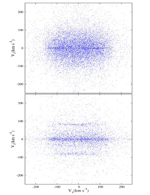
Figure 1: Stellar kinematic distribution in the velocity space, as seen by an observer at $15{\rm\,kpc}$ from the halo center, for a spherical NFW halo + Miyamoto-Nagai disk (top panel), and for a triaxial NFW halo + Miyamoto-Nagai disk (bottom panel).

3.1.1 Changing the axes.

The previous axes choice for the triaxial dark matter halo allows us to compare with the results of paper I.

Now we change the axes ratios (a = 1.47, b = 0.97, c = 0.48), and orientate the disk and the dark matter halo according to the halo model that fits better the Sagittarius stream (Law et al., 2009). In this way the minor and major axes lie in the galactic plane with the intermediate axis perpendicular to the disk and with the new values af the axes we obtain, $b_{p}/a_{p}=0.83$ and $c_{p}/a_{p}=0.67$, corresponding to the axis ratios of the potential.

Figure 2 shows the result of this experiment, with an orientation of the axes different from the treated above but motivated by observational constraints. The track of the halo triaxiality is even more visible for this particular orientation as now four horizontal bands develop in the kinematic stellar structure. Applying the stellar orbit classifier to one of this bands, that with $V_{y}\approx 50{\rm\,km\,s^{-1}}$, we can establish a resonant origin for these structures.

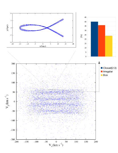
Figure 2: $V_{x}$-$V_{y}$ projection of the velocity space as seen by a hypothetical observer placed at $15{\rm\,kpc}$ from the center in the case of a NFW triaxial halo + Miyamoto-Nagai disk with the axes orientation taken from Law et al. (2009). The histogram shows the result of applying a spectral orbital classifier were we see that the regions more densely populated correspond to resonances. This supports the interpretation that the kinematic structure has a resonant origin. The upper inset shows the orbit of a single particle inside one of these resonant regions.

Comparing Figures 1 (bottom panel) and 2, the differences in the kinematics induced by the two configurations is noticeable. Both, however contain resonant orbits in spite the different orientations of the halo relative to the disk.

3.2 Kuzmin disk with MOND

In this section we describe the numerical simulations carried out considering a Kuzmin disk within MOND theory (Milgrom, 1983) as an alternative to dark matter.

In this theory, dark matter does not exist at all. Instead it is proposed that Newtonian dynamics should be modified to explain observations. In the MOND version, gravity law has a more general form,

$$\mu({g\over a_{0}})g={GM\over r^{2}},$$ (7)

where $a_{0}$ is a universal constant that determines the transition between the regime of strong and weak field and its value is approximately $1.2\times 10^{-10}$ m s^-2. The function $\mu(x)$ is not determined in this theory, but it must satisfy the condition $\mu(x)\approx 1$ when $x\gg 1$ and $\mu(x)\approx x$ when $x\ll 1$.

In the outer part of the galaxies, the weak field regime is valid and $\mu(x)\approx x$. This leads to a rotation velocity $v={(GMa_{0})}^{1/4}$, therefore, the rotation velocity in the outer part of galaxies is independent of $r$. Thus MOND can explain the flattening of the rotation curve at great distances from the center of the galaxies without invoking the existence of dark matter. This is its main achievement and one of the the reasons it was born.

However MOND also has several problems, especially to correctly describe the dynamics of galaxy clusters, for example (Sanders, 1999; Clowe et al., 2004). Nevertheless, despite that dark matter is the most accepted theory, MOND (or modifications of it), has not been totally ruled out.

For this purpose we construct initial conditions in the same way as in the cases of the triaxial halo and a disk: $2\times 10^{6}$ stars within a sphere of $1{\rm\,kpc}$ radius but with the observer neighbourhood centered at ($x=15$  kpc, $y=0$, $z=0$), with random velocities between zero and the escape velocity.

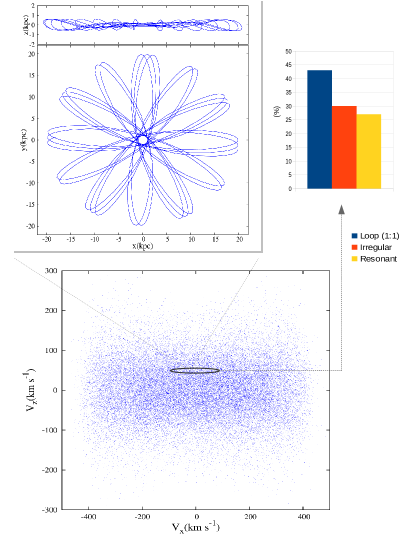
Figure 3: $V_{x}-V_{z}$ projection of the stellar kinematic distribution for a Kuzmin disk within MOND theory. The histogram shows the result of the orbit classification. The upper inset shows a loop orbit in its projections $x-y$ and $x-z$ for a single particle inside the classified region.

We analyze the resulting velocity space after an integration time of 12 gigayears. Figure 3 shows the kinematic structure for this case. An area of higher density in velocity space is formed, but without the symmetric bands that characterize the case of a triaxial halo.

As shown also in Figure 3, a classification of orbits give us more information about the kinematic structure, with no presence of stellar groups and dominated by loop orbits.

Although the geometry of the kinematic structure is preserved regardless of the detailed model of the disk, nevertheless, we decided to repeat the calculations with a Kuzmin disk within a triaxial halo with newtonian gravity and found that the structure is very similar to the one shown in Figure 2, where we used a Miyamoto-Nagai disk, we show this result in Figure 4.

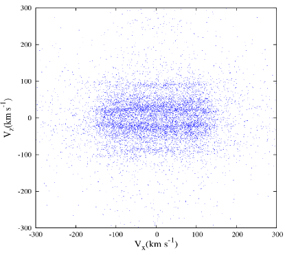
Figure 4: $V_{x}-V_{z}$ projection of the stellar kinematic distribution for a triaxial halo with a Kuzmin disk within Newtonian gravity. The presence of kinematic structures is clear in this plot.

4 Generalized Initial Conditions

As described above the initial conditions set-up, used in the previous sections and in paper I, provide an observer, with a good kinematic accuracy, only inside a limited vicinity, and avoiding to populate the whole halo with particles, ensures a relatively low computing cost. However, this initial distribution of particles is not isotropic around the halo center and the question remains about whether this choice for the initial conditions has a non-negligible effect on the final kinematic structure for the triaxial dark matter halo employed in paper I. With this in mind we introduced a more general and complete initial conditions set-up, different to the described above.

In order to do this, we consider initial conditions with spherical symmetry around the halo center populating the entire simulated domain. This is done by increasing the number of particles which are distributed inside a sphere of $25{\rm\,kpc}$ of radius centered at $(x=0,y=0,z=0)$. The velocities were selected randomly between zero and the local escape velocity.

Although computationally expensive, sampling the entire halo and increasing the number of particles give us a more conclusive mapping of the gravitational potential to establish its relationship with the distribution of stars in velocity space. The choice for the initial conditions ensures that the kinematic stellar structure is not due to the sampling but due to the physical system.

With these new initial conditions, we now repeat the experiment of paper I with just a triaxial NFW halo. Finally, a different density profile for the dark matter halo motivated within the scalar field dark matter model is also employed. The generation of stellar groups within these two, very different in nature, triaxial halo potentials allow us to establish its origin in the triaxiality of the halo rather than in the dark matter nature.

4.1 Triaxial NFW halo

In this experiment we use the potential of equation (1) with parameters $(a=1.47,b=1.22,c=0.98)$ for the axis of the triaxial halo.

We used the generalized initial conditions described above, $16\times 10^{6}$ particles populating a sphere of $25{\rm\,kpc}$ of radius centered at $(x=0,y=0,z=0)$ with velocities selected randomly between zero and the local escape velocity. The system evolves $12{\rm\,Gyr}$.

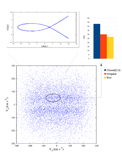
Figure 5: $V_{x}$-$V_{z}$ projection of the velocity space as seen by a hypothetical observer in the case of a NFW triaxial halo. After evolving for about 12 Gyr, we found kinematic structure as seen in paper I, even with the different initial conditions. The histograms show the result of applying a spectral orbital method were we see that the regions more densely populated correspond to resonances. This supports the interpretation that the kinematic structure has a resonant origin. The upper inset shows the orbit of a single particle inside one of these resonant regions.

Figure 5 shows the $V_{x}$-$V_{z}$ projection of the velocity space at the end of the integration time as seen by a hypothetical observer placed at $15{\rm\,kpc}$ from the halo center. Overdensities are distinguishable in the kinematic structure, mostly around $Vz\approx 45{\rm\,km\,s^{-1}}$ and $Vz\approx-45{\rm\,km\,s^{-1}}$. By doing a classification of orbits one can notice that these overdensities have a resonant origin and its independent of the initial conditions.

4.2 Triaxial scalar field dark matter halo

For this triaxial halo (equation 3) we used the generalized initial conditions described above, $12\times 10^{6}$ particles populating a sphere of $25{\rm\,kpc}$ of radius centered at $(x=0,y=0,z=0)$, with velocities selected randomly between zero and the local escape velocity.

We selected $(a=1.47,b=1.22,c=0.98)$ for the triaxial halo axes, and evolved the system for $12$  Gyr. Figure 6 shows the $V_{x}$-$V_{z}$ projection of the velocity space at the end of the integration time, as seen by a hypothetical observer placed at $8.5{\rm\,kpc}$ from the halo center.

In figure 6 we found horizontal structure resembling that seen in our previous experiments. We also performed a simulation with the spherical case $(a=1,b=1,c=1)$ for comparison, and found that the velocity space is featureless and homogeneous. This suggests that the kinematic structure seen in the velocity space of the triaxial halo corresponds, again, to stars librating in the vicinity of resonances. We verified this by using the spectral orbital method of Carpintero & Aguilar (1998), finding that the most remarkable regions of the velocity space are dominated by resonant orbits.

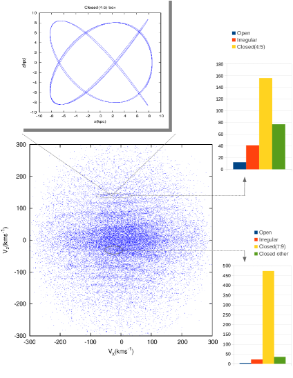
Figure 6: $v_{x}$-$v_{z}$ projection of the velocity space as seen by a hypothetical observer in the case of the scalar field triaxial halo. After evolving for about 12 Gyr, we found kinematic structure as seen in paper I, even with the randomly selected velocities and homogeneous initial particle distribution around the halo center. The histograms showed here are the result of applying a spectral orbital method, where regions more densely populated, correspond to resonances. The upper inset shows the orbit of a single particle inside one of these resonant regions.

In figure 7 we show the $V_{x}$-$V_{y}$ projection for another measure of the data but now moving the hypothetical observer to a distance of $20{\rm\,kpc}$ from the halo center. At this distance we found again a horizontal pattern as in the figures before which means that the effect of triaxiality acts across the entire stellar halo. Again by applying the spectral orbital method we can see that dark matter halo resonances are able to densely populate the stellar velocity space with this characteristic horizontal pattern.

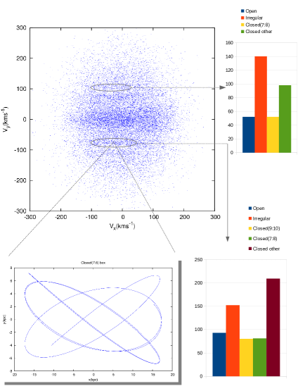
Figure 7: $v_{x}$-$v_{y}$ projection of the velocity space as seen by a hypothetical observer in the case of the scalar field triaxial halo. Taken from the same simulation as before but this time the observer is placed at a distance of $20{\rm\,kpc}$ from the halo center. The histograms showed are the result of applying a spectral orbital method were we see that the regions more densely populated correspond to resonances. This supports the interpretation that the kinematic structure has a resonant origin. The bottom inset shows the orbit of a single particle inside one of these resonant regions.

5 Discussion and Conclusions

In this work we extend the orbital study of a stellar system under the influence of the gravitational potential generated by a steady triaxial dark matter halo, compared to spherical ones as in Paper I (Rojas-Niño et al., 2012). We now have added a Milky-Way-like disk to our study in order to investigate for a way to separate the effects from a non-spherical halo and a disk. We have also tested a different type of dark matter halo profile based on theories of scalar field dark matter. Finally, we have included a Kuzmin disk assuming a MOND gravity theory in order to test the consequences on the orbital behaviour and the possible production of moving groups.

We show that, independently of the nature of dark matter, a non-spherical shape of the Milky Way dark matter halo, influences strongly the stellar halo kinematic structure, as seen from the long lasting resonant features formed in simulations. As it was pointed out in Paper I, there is an enormous difference with the spherical case, where no kinematic structure is triggered. We have explored also with a different halo profile motivated by the scalar field dark matter model with an important feature, the presence of density wiggles, characteristic oscillations of scalar field configurations. We conclude that this scalar field density wiggles are unable to trigger any moving groups in the spherical case. However in the triaxial case, this profile produces structures with the same resonant origin as in the typical NFW triaxial halos.

We also confirm that the structures seen in the velocity space for triaxial halos, do not depend on the initial conditions, the effect is still present in spite of the two different initial distributions strategies of particles used in this paper. The fact that the kinematic structure is independent from the initial conditions makes stronger the resonant nature versus an incomplete relaxation of initial conditions. Our IC´s strategy is motivated by the fact that there are not selfconsistent phase space distribution for triaxial halos, it can be argued that incomplete relaxation is producing the kinematic structure reported in this paper. However the fact that such structure is produced only in the non-spherical case, and lasts for longer than the Universe age, and is not altered by the stellar disk presence makes our conclusions robust.

In this work a disk potential was introduced in order to understand whether this component is able to erase the orbital structure produced by a triaxial halo, or if the disk itself could produce moving groups in the halo that can be erroneously taken as the ones produced by a triaxial halo. With this study we learnt that the disk influence is only important close to it, and that it is unable to erase the orbital structure induced by the halo in all cases we studied. In the same manner, we studied the effect of the disk on the production of kinematic structures in the halo, and we found that for an axisymmetric disk, there are no dominant resonant structures (moving groups). Although it is known that non-axisymmetric structures (such as spiral arms and bars) in the disk, may produce important kinematic structure into galactic disks, their influence diminishes fast out of the disk plane.

Finally, we have also tested the results comparing with a modified gravity model (MOND), with a Kuzmin disk. We find in this case no kinematic structure at all.

In the close future we will be likely able to distinguish, for instance, satellite remnants groups originated from a single event from these associated with the dark matter halo shape with the help of the stellar population data. The great surveys such as Gaia, SDSS, etc., will allow us the detection of these type of kinematic groups, which would be a clear indication of the triaxiality (non-sphericity) of the Milky Way dark matter halo, and will be of great importance for the galaxy formation theories and the $\Lambda$CDM scenario.

References

- Allen & Santillán (1991) Allen, C. & Santillán, A. 1991, Rev. Mexicana Astron. Astrofis., 22, 255
- Allgood et al. (2006) Allgood, B., Flores, R. A., Primack, J. R., et al. 2006, MNRAS, 367, 1781
- Avila-Reese (2006) Avila-Reese, V. 2006, arXiv:astro-ph/0605212
- Carpintero & Aguilar (1998) Carpintero, D. D., & Aguilar, L. A. 1998, MNRAS, 298, 1
- Clowe et al. (2004) Clowe, D., Gonzalez A. & Markevitch, M. 2004, Ap J 604, 596.
- Chandrasekhar (1969) Chandrasekhar S., 1969, Ellipsoidal Figures of Equilibrium, The Silliman Foundation Lectures. Yale Univ. Press, New Haven
- Debattista et al. (2013) Debattista, V. P., Roškar, R., Valluri, M., et al. 2013, MNRAS, 434, 2971
- Deg & Widrow (2013) Deg, N., & Widrow, L. 2013, MNRAS, 428, 912
- Ghigna et al. (1998) Ghigna, S., Moore, B., Governato, F., Lake, G., Quinn, T., & Stadel, J. 1998, MNRAS, 300, 146
- Gnedin et al. (2005) Gnedin, O. Y., Gould, A., Miralda-Escudé, J., & Zentner, A. R. 2005, ApJ, 634, 344
- Gnedin et al. (2006) Gnedin, O., Weinberg, D. H., Pizagno, J., Prada, F., Rix, H. W. 2006, a-ph0607394
- González-Morales et al. (2013) González-Morales, A. X., Diez-Tejedor, A., Ureña-López, L. A., & Valenzuela, O. 2013, Phys. Rev. D, 87, 021301
- Governato et al. (2012) Governato, F., Zolotov, A., Pontzen, A., et al. 2012, MNRAS, 422, 1231
- Guzmán & Matos (2000) Guzmán F. S., Matos T., 2000, Class. Quantum Grav., 17, L9-L16.
- Jing & Suto (2002) Jing, Y. P., & Suto, Y. 2002, ApJ, 574, 538
- Kalirai (2012) Kalirai, J. S. 2012, Nature, 486, 90
- Kauffmann et al. (1993) Kauffmann, G., White, S. D. M., & Guideroni, B. 1993, MNRAS, 264, 201 Klypin, A.A., Kravtsov, A.V., Valenzuela, O., & Prada, F. 1999, ApJ, 522, 82
- Klypin et al. (1999) Klypin, A., Gottlöber, S., Kravtsov, A. V., & Khokhlov, A. M. 1999, ApJ, 516, 530
- Law et al. (2009) Law, D. R., Majewski, S. R., & Johnston, K. V. 2009, ApJ, 703, L67
- Loebman et al. (2012) Loebman, S. R., Ivezić, Ž., Quinn, T. R., et al. 2012, ApJ, 758, L23
- Loebman et al. (2014) Loebman, S. R., Ivezić, Ž., Quinn, T. R., et al. 2014, ApJ, 794, 151
- Lux et al. (2012) Lux, H., Read, J. I., Lake, G., & Johnston, K. V. 2012, MNRAS, L464
- Magaña et al. (2012) J. Magaña and T. Matos, J. Phys. Conf. Ser. 378, 012012 (2012)
- Martínez-Medina & Matos (2014) Martinez-Medina L. A., Matos T., 2014, MNRAS, 444 (3), 185-191
- Miyamoto & Nagai (1975) Miyamoto, M., & Nagai, R. 1975, PASJ, 27, 533
- Milgrom (1983) Milgrom, M. 1983, ApJ, 270, 365
- Moore et al. (1999) Moore, B., Ghigna, S., Governato, F., et al. 1999, ApJ, 524, L19
- Moore (1994) Moore, B. 1994, Nature, 370, 629
- Navarro et al. (1996) Navarro, J. F., Frenk, C. S., & White, S. D. M. 1996, ApJ, 462, 563
- Peñarrubia et al. (2009) Peñarrubia, J., Walker, M. G., & Gilmore, G. 2009, MNRAS, 399, 1275
- Pizagno et al. (2007) Pizagno, J., et al. 2007, AJ, 134, 945
- Press et al. (1992) Press, W. H., Teukolsky, S. A., Vetterling, W. T., & Flannery, B. P. 1992, Numerical Recipes in Fortran 77: The Art of Scientific Computing (2d ed.; Cambridge: Cambridge Univ. Press)
- Robles & Matos (2013) Robles V. H., Matos T., 2013, ApJ, 763, 19
- Rojas-Niño et al. (2012) Rojas-Niño, A., Valenzuela, O., Pichardo, B., & Aguilar, L. A. 2012, ApJ, 757, L28
- Read & Moore (2005) Read, J. I., Moore, B. 2005, MNRAS, 361, 971
- Sanders (1999) R.H. Sanders, Astrophys. J. 512, L23 (1999).
- Steffen & Valenzuela (2008) Steffen, J. H., & Valenzuela, O. 2008, MNRAS, 387, 1199
- Valenzuela et al. (2007) Valenzuela, O., Rhee, G., Klypin, A., Governato, F., Stinson, G., Quinn, T., & Wadsley, J. 2007, ApJ, 657, 773
- Valenzuela et al. (2014) Valenzuela, O., Hernandez-Toledo, H., Cano, M., et al. 2014, AJ, 147, 27
- Valluri et al. (2012) Valluri, M., Debattista, V. P., Quinn, T. R., Roškar, R., & Wadsley, J. 2012, MNRAS, 419, 1951
- Van den Bosch (1998) Van den Bosch, F. C. 1998, ApJ, 507, 601
- Vera-Ciro et al. (2011) Vera-Ciro, C. A., Sales, L. V., Helmi, A., et al. 2011, MNRAS, 416, 1377
- Vera-Ciro (2014) Vera-Ciro C. A., Sales L. V., Helmi A., Navarro J. F., 2014, MNRAS, 439, 2863
- White & Rees (1978) White, S. D. M., & Rees, M. J. 1978, MNRAS, 183, 341
- Zentner et al. (2005) Zentner, A. R., Kravtsov, A. V., Gnedin, O. Y., & Klypin, A. A. 2005, ApJ, 629, 219