$B$-meson decay constants: a more complete picture from full lattice QCD

Abstract

We extend the picture of $B$-meson decay constants obtained in lattice QCD beyond those of the $B$, $B_{s}$ and $B_{c}$ to give the first full lattice QCD results for the $B^{*}$, $B^{*}_{s}$ and $B^{*}_{c}$. We use improved NonRelativistic QCD for the valence $b$ quark and the Highly Improved Staggered Quark (HISQ) action for the lighter quarks on gluon field configurations that include the effect of $u/d$, $s$ and $c$ quarks in the sea with $u/d$ quark masses going down to physical values. For the ratio of vector to pseudoscalar decay constants, we find $f_{B^{*}}/f_{B}$ = 0.941(26), $f_{B^{*}_{s}}/f_{B_{s}}$ = 0.953(23) (both $2\sigma$ less than 1.0) and $f_{B^{*}_{c}}/f_{B_{c}}$ = 0.988(27). Taking correlated uncertainties into account we see clear indications that the ratio increases as the mass of the lighter quark increases. We compare our results to those using the HISQ formalism for all quarks and find good agreement both on decay constant values when the heaviest quark is a $b$ and on the dependence on the mass of the heaviest quark in the region of the $b$. Finally, we give an overview plot of decay constants for gold-plated mesons, the most complete picture of these hadronic parameters to date.

I Introduction

Lattice QCD calculations are now an essential part of $B$ physics phenomenology (see for example Davies (2011)), providing increasingly precise determinations of decay constants, form factors and mixing parameters needed, along with experiment, in the determination of Cabibbo-Kobayashi-Maskawa (CKM) matrix elements. As the constraints being provided by lattice QCD become more stringent it is increasingly important to expand the range of hadronic matrix elements being calculated to allow tests both against experiment where possible and/or against expectations from other approaches. Decay constants are particularly useful in this respect because they are single numbers expressing the amplitude for a meson to annihilate to a single particle (for example a $W$ boson or a photon), encapsulating information about its internal structure. They are straightforwardly calculated in lattice QCD from the same hadron correlation functions being used to determine the hadron masses. The only additional complication is that normalisation of the appropriate operator for the meson creation/annihilation is required. In this way we can build up a tested and consistent ‘big picture’ of meson decay constants within which sit the results being used for CKM element determination.

To this end we determine here the decay constants that parameterise the amplitude to annihilate for the vector mesons $B^{*}$ and $B_{s}^{*}$. These mesons are the partners of the $B$ and $B_{s}$ whose weak decay matrix elements are critical to understanding heavy flavour physics. Decay modes of the $B^{*}$ and $B_{s}^{*}$ are dominated by electromagnetic radiative decays Olive et al. (2014) to $B$ and $B_{s}$, however, and so it is unlikely that processes in which the decay constant is the key hadronic parameter will be measured experimentally. The determination of the vector decay constants is nevertheless useful because the relationship with that of the pseudoscalar decay constant can be understood within the framework of Heavy Quark Effective Theory (HQET) and the decay constants appear in phenomenological analyses of the vector form factor for semileptonic decay processes for the pseudoscalar mesons (see Becirevic et al. (2014) for a recent discussion of this).

Since vector and pseudoscalar heavy-light mesons differ only in their internal spin configuration, their decay constants might be expected to have rather similar values. The key question is then: by how much do they differ and which is larger? A recent review Lucha et al. (2014a) showed tension between the results for the ratio of the $B^{*}$ to $B$ decay constants from QCD sum rules and from lattice QCD. The lattice QCD results used $u/d$ quarks (only) in the sea and obtained results for mesons containing $b$ quarks from an interpolation between results for quarks close to the $c$ mass and the static (infinite mass) limit Becirevic et al. (2014). This gave a result for the ratio greater than 1 whereas the QCD sum rules approach quoted preferred a value less than 1.

The results we give here build on our state-of-the-art calculation of the $B$ and $B_{s}$ decay constants Dowdall et al. (2013a) using an improved NonRelativistic QCD (NRQCD) formulation Dowdall et al. (2012a) that allows us to work to high accuracy directly at the $b$ quark mass. We also use lattice QCD gluon field configurations that have the most realistic QCD vacuum to date, include $u/d$, $s$ and $c$ quarks in the sea (using the Highly Improved Staggered Quark formalism Follana et al. (2007)) with the $u/d$ quark mass taking values down to the physical value. We therefore avoid significant systematic errors from extrapolations in the $u/d$ quark mass. We are able to give results for the ratio of vector to pseudoscalar decay constants for both the $B_{s}$ and the $B$ and the SU(3)-breaking ratio of these ratios. We find clearly that the vector decay constant is smaller than the pseudoscalar decay constant in both cases.

We also give results for the decay constant of the $B_{c}$ meson and its vector partner the $B_{c}^{*}$. The $B_{c}$ has been seen experimentally only relatively recently Olive et al. (2014) and is interesting because it can be viewed both as a heavy-heavy meson and as a heavy-light meson. Here we compare its ratio of vector to pseudoscalar decay constants to that of the $B$ and $B_{s}$, and find the ratio is significantly larger, now being very close to 1.

The decay constant of the $B_{c}$ is quite different from that of the $B$ and $B_{s}$, being nearly double their size. The $B_{c}$ decay constant can be used to predict its partial width for leptonic decay that may be observed in the future. We determine this decay constant here using NRQCD $b$ quarks and HISQ $c$ quarks and compare to our previous result McNeile et al. (2012a) that used the HISQ action for both quarks and mapped out the behaviour of a range of decay constants for valence heavy quarks in the region between the $c$ quark mass and the $b$ quark mass. Since the HISQ action is fully relativistic this is a good test of our understanding of systematic errors in lattice QCD, and confirmation of how well improved actions work.

In a further study of this point we go on to look at the dependence of decay constants on the valence heavy quark mass using quark masses lighter than that of the $b$ in the NRQCD action. This enables us to compare both the value of specific decay constants and the dependence on the heavy quark mass with that from using the relativistic HISQ action. We also demonstrate the consistency of our results for the ratio of vector to pseudoscalar decay constants for the $B_{s}$ meson here to our earlier result for the same ratio for the $D_{s}$ meson Donald et al. (2014a) using HISQ quarks.

A very consistent picture thus emerges from both a nonrelativistic and a relativistic approach to heavy quarks within lattice QCD. Both approaches are the result of several stages of improvement to reduce discretisation errors and other systematic uncertainties to a low level, important for making a detailed comparison.

We begin by outlining the methods used in our lattice calculation, which follow Dowdall et al. (2013a, 2012b). Section III.1 gives results for the decay constants of the $B_{s}^{*}$ and $B^{*}$ and their comparison, and then section III.4 gives results for the decay constants of the $B_{c}$ and the $B_{c}^{*}$. Section III.5 works with quarks lighter than $b$ to demonstrate the heavy quark mass dependence of the decay constants and compare to our earlier results using the HISQ formalism for $b$ quarks. Section IV compares our results for vector meson decay constants to those of earlier determinations using other methods, including HQET arguments, and shows how the $B_{c}$ fits in between results for heavyonium and heavy-light mesons. Section V gives our conclusions, including the promised ‘big picture’ for the decay constants of gold-plated mesons from lattice QCD, the most complete picture of these hadronic parameters to date.

II Lattice calculation

Since the first lattice NRQCD calculations were done for heavy-light mesons Davies (1993), huge improvements have been made. The current state-of-the-art Dowdall et al. (2013a, 2012b) uses an improved NRQCD action for the heavy quark coupled to a HISQ light quark on gluon configurations that include an improved gluon action and HISQ sea quarks. Here we extend these calculations to include the decay constants of vector heavy-light mesons.

The gluon field configurations that we use were generated by the MILC collaboration Bazavov et al. (2010, 2013). These are $n_{f}=2+1+1$ configurations that include the effect of light (up/down), strange and charm quarks in the sea with the HISQ action Follana et al. (2007, 2008) and a Symanzik improved gluon action with coefficients correct through $\mathcal{O}(\alpha_{s}a^{2},n_{f}\alpha_{s}a^{2})$ Hart et al. (2009). The lattice spacing values that we use range from $a=0.15$ fm to $a=0.09$ fm. The configurations have well-tuned sea strange quark masses and sea light quark masses ($m_{u}=m_{d}=m_{l}$) with ratios to the strange mass from $m_{l}/m_{s}=0.2$ down to the value that corresponds to the experimental $\pi$ meson mass of $m_{l}/m_{s}=1/27.4$ Bazavov et al. (2014).

In Dowdall et al. (2012a) we accurately determined the lattice spacings using the mass difference of the $\Upsilon^{\prime}$ and $\Upsilon$ mesons using the same NRQCD action for the $b$ quark as we use here. The details of each ensemble, including the lattice spacing, sea quark masses and spatial volumes, are given in table 1. All ensembles were fixed to Coulomb gauge.

Table 1: Details of the ensembles (sets) of gauge field configurations used in this calculation Bazavov et al. (2010, 2013). $\beta$ is the bare gauge coupling, $a_{\Upsilon}$ is the lattice spacing as determined by the $\Upsilon(2S-1S)$ splitting in Dowdall et al. (2012a), where the three errors are statistics, NRQCD systematics and experiment. Column 4 gives the corresponding values of $\alpha_{s}$ used in renormalisation factors. This is taken as $\alpha_{V}(n_{f}=4,q=2/a)$ and determined from McNeile et al. (2010); Chakraborty et al. (2015). $am_{l},am_{s}$ and $am_{c}$ are the sea quark masses in lattice units. We also give, in column 8, values for $\delta x_{\mathrm{sea}}$, the fractional difference in the sum of the light quark masses from their physical values. $\delta x_{\mathrm{sea}}$ is defined as $(2m_{l}+m_{s})/(2m_{l,\mathrm{phys}}+m_{s,\mathrm{phys}})-1$, using values of $m_{s,\mathrm{phys}}$ from Dowdall et al. (2012a) and $m_{s}/m_{l}=27.4$ Bazavov et al. (2014). $L/a\times T/a$ gives the spatial and temporal extent of the lattices and $n_{{\rm cfg}}$ is the number of configurations in each ensemble. 16 time sources were used for the valence quark propagators on each configuration for increased statistics. Sets 1, 2 and 3 will be referred to in the text as “very coarse”, 4, 5 and 6 as “coarse” and 7 as “fine”. Sets 3 and 6 include light sea quarks with their physical masses.

Set	$\beta$	$a_{\Upsilon}$ (fm)	$\alpha_{V}(2/a)$	$am_{l}$	$am_{s}$	$am_{c}$	$\delta x_{\mathrm{sea}}$	$L/a\times T/a$	$n_{{\rm cfg}}$
1	5.80	0.1474(5)(14)(2)	0.346	0.013	0.065	0.838	0.323	16$\times$48	1020
2	5.80	0.1463(3)(14)(2)	0.344	0.0064	0.064	0.828	0.126	24$\times$48	1000
3	5.80	0.1450(3)(14)(2)	0.343	0.00235	0.0647	0.831	0.027	32$\times$48	1000
4	6.00	0.1219(2)(9)(2)	0.311	0.0102	0.0509	0.635	0.259	24$\times$64	1052
5	6.00	0.1195(3)(9)(2)	0.308	0.00507	0.0507	0.628	0.108	32$\times$64	1000
6	6.00	0.1189(2)(9)(2)	0.307	0.00184	0.0507	0.628	-0.004	48$\times$64	1000
7	6.30	0.0884(3)(5)(1)	0.267	0.0074	0.0370	0.440	0.327	32$\times$96	1008

II.1 NRQCD valence quarks

We use improved NRQCD for the $b$ quark, which takes advantage of the nonrelativistic nature of the $b$ quark within its bound states for very good control of discretisation uncertainties. This allows us to work with relatively low numerical cost on the lattices with the lattice spacing values given above. NRQCD has the advantage that the same action can be used for both bottomonium and $B$-meson calculations so that tuning of the $b$-quark mass and determination of the lattice spacing can be done using bottomonium and there are no new parameters to be tuned at all for $B$-mesons. $b$-quark propagators are calculated in NRQCD by evolving forward in time (using eq. (2)) from a starting condition. This is numerically very fast and high statistics can then readily be accumulated for precise results. The action used here builds on the standard NRQCD action Lepage et al. (1992) accurate through $v^{4}$ in the heavy quark velocity $v$ (using power-counting terminology for bottomonium) by including one loop radiative corrections to many of the $v^{4}$ coefficients Hammant et al. (2011); Dowdall et al. (2012a). We studied the effect of these improvements on the bottomonium spectrum in Dowdall et al. (2012a); Daldrop et al. (2012); Dowdall et al. (2014) and in $B$, $B_{s}$ and $B_{c}$ meson masses in Dowdall et al. (2012b).

The NRQCD Hamiltonian we use is given by Lepage et al. (1992):

$$e^{-aH} = \left(1-\frac{a\delta H}{2}\right)\left(1-\frac{aH_{0}}{2n}\right)^{n}U_{t}^{{\dagger}}$$ (1)

$$\times\left(1-\frac{aH_{0}}{2n}\right)^{n}\left(1-\frac{a\delta H}{2}\right)$$

with

$$aH_{0} = -\frac{\Delta^{(2)}}{2am_{b}},$$

$$a\delta H = -c_{1}\frac{(\Delta^{(2)})^{2}}{8(am_{b})^{3}}+c_{2}\frac{i}{8(am_{b})^{2}}\left(\bf{\nabla}\cdot\tilde{\bf{E}}\right.-\left.\tilde{\bf{E}}\cdot\bf{\nabla}\right)$$ (2)

$$-c_{3}\frac{1}{8(am_{b})^{2}}\bf{\sigma}\cdot\left(\tilde{\bf{\nabla}}\times\tilde{\bf{E}}\right.-\left.\tilde{\bf{E}}\times\tilde{\bf{\nabla}}\right)$$

$$-c_{4}\frac{1}{2am_{b}}\,{\bf{\sigma}}\cdot\tilde{\bf{B}}+c_{5}\frac{\Delta^{(4)}}{24am_{b}}$$

$$-c_{6}\frac{(\Delta^{(2)})^{2}}{16n(am_{b})^{2}}.$$

Here $\nabla$ is the symmetric lattice derivative and $\Delta^{(2)}$ and $\Delta^{(4)}$ the lattice discretization of the continuum $\sum_{i}D_{i}^{2}$ and $\sum_{i}D_{i}^{4}$ respectively. $am_{b}$ is the bare $b$ quark mass. The parameter $n$ has no physical significance, but is included for numerical stability of high momentum modes. We take the value $n=4$ here in all cases. $\bf\tilde{E}$ and $\bf\tilde{B}$ are the chromoelectric and chromomagnetic fields calculated from an improved clover term Gray et al. (2005). The $\bf\tilde{B}$ and $\bf\tilde{E}$ are made anti-hermitian but not explicitly traceless, to match the perturbative calculations done using this action.

The coefficients $c_{i}$ in the action are unity at tree level but radiative corrections cause them to depend on $am_{b}$ at higher orders in $\alpha_{s}$. These were calculated for the relevant $b$ quark masses using lattice perturbation theory in Dowdall et al. (2012a); Hammant et al. (2011) and the values used in this paper are given in Table 2. Including the one-loop radiative corrections to $c_{4}$ is particularly important here, since this coefficient controls the hyperfine splitting between the vector and pseudoscalar states. We showed in Dowdall et al. (2012b) that improving $c_{4}$ leads to accurate results for $b$-light hyperfine splittings in keeping with the results of Dowdall et al. (2012a) for bottomonium. Most of the correlators we use here for determining the vector heavy-light meson decay constants come from the same calculation as that of Dowdall et al. (2012b).

The tuning of the $b$ quark mass on these ensembles was discussed in Dowdall et al. (2012a). We use the spin-averaged kinetic mass of the $\Upsilon$ and $\eta_{b}$ and tune this to an experimental value of 9.445(2) GeV. This allows for electromagnetism and $\eta_{b}$ annihilation effects missing from our calculation Gregory et al. (2011). Note that we no longer have to apply a shift for missing charm quarks in the sea Gregory et al. (2011). The values used in this calculation are the same as those in Dowdall et al. (2012b, 2013a) and given in table 1 along with other parameters.

Table 2: The coefficients $c_{1}$, $c_{5}$, $c_{4}$ and $c_{6}$ used in the NRQCD action (eq. (2)) for the values of the $b$ quark mass corresponding to those in 1. $c_{2}$ and $c_{3}$ are set to 1.0.

Set	$c_{1}$	$c_{5}$	$c_{4}$	$c_{6}$
very coarse	1.36	1.21	1.22	1.36
coarse	1.31	1.16	1.20	1.31
fine	1.21	1.12	1.16	1.21

Table 3: Parameters used in the NRQCD action. $am_{b}$ is the bare $b$ quark mass and $u_{0L}$ the Landau link tadpole-improvement factor used in the NRQCD action Lepage and Mackenzie (1993). $\delta x_{b}$ gives the fractional mistuning in the $b$ quark mass ($(am_{b}-am_{b,\mathrm{phys}})/am_{b,\mathrm{phys}}$) obtained from the determination of the spin-averaged kinetic mass of the $\Upsilon$ and $\eta_{b}$ Dowdall et al. (2012a), when this has a magnitude larger than 0.5%. The column $a_{\mathrm{sm}}$ gives the size parameters of the quark smearing functions (see section II.3 and Dowdall et al. (2012b)), which take the form $\exp(-r/a_{\mathrm{sm}})$. $a_{\mathrm{sm}}$ is kept approximately constant in physical units .

Set	$am_{b}$	$\delta x_{b}$	$u_{0L}$	$a_{\mathrm{sm}}/a$
1	3.297	0	0.81950	2.0,4.0
2	3.263	0	0.82015	2.0,4.0
3	3.25	0.005	0.81947	2.0,4.0
4	2.66	-0.013	0.8340	2.5,5.0
5	2.62	0	0.8349	2.0,4.0
6	2.62	0	0.8341	2.0,4.0
7	1.91	0.009	0.8525	3.425,6.85

We end this section with a brief discussion of the assessment and removal of discretisation errors in a calculation that uses NRQCD Dowdall et al. (2012a). A typical procedure to remove finite-$a$ errors in a lattice QCD calculation consists of :

• assume that the error is given by a function with leading term $ca^{2}$ (for suitably accurate actions)

• perform calculations at multiple values of $a$

• determine the unknown parameter $c$ above by fitting the results as a function of $a$

• subtract the fitted error function to obtain a physical result.

The first step of the procedure changes for NRQCD, because the error function must be more complicated. The coefficient of $a^{2}$ errors will be in general a function $c(am_{b})$. This function is not known but varies slowly with $am_{b}$ for $am_{b}>1$. It can therefore be approximated by a simple polynomial in $am_{b}$ for the range of values of $am_{b}$ used here, which are all larger than 1. Note that this polynomial approximation is not valid as $am_{b}\rightarrow 0$, but the procedure only requires that it be valid over the range used for our results. Our fit to the $a$-dependence of our results, to be discussed further in Section III, then has additional parameters to allow for the $a$-dependence coming from NRQCD (we also have simpler $a$-dependence coming from the gluon and light quark actions). The final physical result then has larger uncertainties because of this but it does allow us to account for NRQCD effects.

II.2 HISQ valence quarks

For the $u/d$, $s$ and $c$ valence quarks in our calculation we use the same HISQ action as for the sea quarks. The advantage of using HISQ is that $am_{q}$ discretisation errors are under sufficient control that it can be used both for light and for $c$ quarks Follana et al. (2007, 2008); Davies et al. (2010a). The HISQ action is also numerically inexpensive which means we are able to perform a very high statistics calculation to combat the signal to noise ratio problems that arise in simulating B-mesons. For example, we use 16 time sources for both NRQCD and HISQ propagators on each configuration, so we are typically generating 16,000 correlators per ensemble.

The masses used on each ensemble are given in table 4. Again these are the same as in Dowdall et al. (2012b, 2013a). In Dowdall et al. (2012a) accurate strange quark masses were determined for each ensemble, tuned from the mass of the $\eta_{s}$ meson, a pseudoscalar $s\overline{s}$ which can be prevented from mixing with other states on the lattice so that its mass can be determined very accurately Davies et al. (2010b). Using experimental $K$ and $\pi$ meson masses we found $M_{\eta_{s}}$ = 0.6893(12) GeV (see also Dowdall et al. (2013b)). The values of $am_{s}^{\mathrm{val}}$ in table 4 correspond to these tuned values. The light valence quarks are taken to have the same masses as in the sea.

Charm quark masses are tuned by matching the mass of the $\eta_{c}$ to experiment. The experimental value is shifted by 2.6 MeV for missing electromagnetic effects and 2.4 MeV for not allowing it to annihilate to gluons, giving 2.985(3) GeV Davies et al. (2010b). The $\epsilon_{\mbox{\tiny Naik}}$ term in the action is not negligible for charm quarks and we use the tree level formula given in Davies et al. (2010a); the values appropriate to our masses are given in table 4.

Table 4: The parameters used in the generation of the HISQ propagators. $am_{l}^{\rm val}$ and $am_{s}^{\rm val}$ are the valence light and strange quark masses respectively, in lattice units. $am_{c}^{\rm val}$ is the charm quark mass in lattice units (only a subset of the ensembles was used in this case) and $\epsilon_{\mbox{\tiny Naik}}$ is the corresponding coefficient of the Naik term in the HISQ action for charm. On set 5 $\epsilon_{\mbox{\tiny Naik}}$ is very slightly wrong - it should be -0.224. The impact of this is negligible.

Set	$am_{l}^{\rm val}$	$am_{s}^{\rm val}$	$am_{c}^{\rm val}$	$\epsilon_{\mbox{\tiny Naik}}$
1	0.013	0.0641	0.826	-0.345
2	0.0064	0.0636	0.818	-0.340
3	0.00235	0.0628	-	-
4	0.01044	0.0522	0.645	-0.235
5	0.00507	0.0505	0.627	-0.222
6	0.00184	0.0507	-	-
7	0.0074	0.0364	0.434	-0.117

II.3 NRQCD-HISQ correlators

The NRQCD $b$ and HISQ $u/d$, $s$ or $c$ light quark propagators are combined into a meson correlation function in a straightforward way. Since staggered quarks have no spin index, staggered quark propagators must first be converted to 4-component ‘naive’ propagators so that they can be combined with quark propagators from other formalism such as NRQCD. To do this, the 4x4 ‘staggering matrix’ $\Omega(x)=\prod_{\mu=0}^{4}(\gamma_{\mu})^{x_{\mu}}$ that was used to convert the naive quark action into the staggered quark action has to be applied to the staggered quark propagator at each end to ‘undo’ the transformation Wingate et al. (2003). The spin and colour components of the naive propagator and the NRQCD propagator can then be tied up at source and sink with appropriate $\gamma$ matrices (taking appropriate $2\times 2$ blocks since the NRQCD propagator is 2-component) to form a pseudoscalar or vector meson correlator. We sum over the spatial sites on the sink time-slice to project onto zero spatial momentum in all cases.

One complication is that ‘random-wall’ sources (i.e. a set of U(1) random numbers over a timeslice) are used for the light quark propagators to improve statistical accuracy in our light meson calculations (see, for example, Dowdall et al. (2013b)). When these propagators are tied together the result is equivalent to having a delta function source at each point on the time-slice. As well as the convenience, statistical accuracy is also improved by re-using these propagators in our heavy-light meson calculations. The source for the NRQCD propagators must then use the same random numbers on the same source time-slice and in addition must also include a spin trace over the staggering matrix and appropriate gamma matrix for a pseudoscalar or vector meson Gregory et al. (2011), i.e. there is a separate NRQCD propagator for each meson that will be made. Combining these NRQCD propagators with the light quark propagators is then equivalent to having a delta function source at each point on the timeslice, as for the light meson case.

A further numerical improvement is to make smeared sources for the NRQCD propagators by convoluting a smearing function with the random-wall source as above. Suitably chosen smearing functions can improve the overlap of the correlator with different states in the spectrum, and this is particularly important for fits to extract radially excited energies Dowdall et al. (2012a). Here we use it to improve the determination of ground-state properties by improving the overlap with the ground-state at early times before the signal/noise ratio has degraded significantly. For each ensemble we then use a local source and 2 smeared sources. The smearing functions were optimised in our heavy-light meson spectrum calculation Dowdall et al. (2012b) and take the form $\exp(-r/a_{sm})$ as a function of radial distance, with two different radial sizes, $a_{sm}$, on each ensemble as given in Table 1.

Propagators were calculated, and meson correlators obtained, using 16 time sources on each configuration. The calculation was also repeated with the heavy quark propagating in the opposite time direction. All correlators from the same configuration were binned together to avoid underestimating the statistical errors. When each smearing is used at source and sink this gives a $3\times 3$ matrix of correlation functions on each ensemble. In addition we have a 3-vector of correlation functions from using each smearing at the source and a relativistic current correction operator at the sink, to be discussed below.

Meson energies and amplitudes are extracted from the meson correlation functions using a simultaneous multi-exponential Bayesian fit Lepage et al. (2002) as a function of time separation between source and sink to the form

$$C_{\rm meson}(i,j,t_{0};t) = \sum^{N_{\exp}}_{k=0}b_{i,k}b^{*}_{j,k}e^{-E_{k}(t-t_{0})}$$

$$- \sum^{N_{\exp}-1}_{k^{\prime}=0}d_{i,k^{\prime}}d^{*}_{j,k^{\prime}}(-1)^{(t-t_{0})}e^{-E^{\prime}_{k^{\prime}}(t-t_{0})}.$$

Here $i$, $j$ label the smearing (or current correction operator) included in the correlator and $k$ labels the set of energy levels for states appearing in the correlator. Here we are concentrating on the properties of the ground-state, $k=0$. $k^{\prime}$ labels a set of opposite-parity states that appear with an oscillating behaviour in time as a result of using staggered quarks. Energies for ground-states, radially excited states and oscillating states were extracted from these correlation functions in Dowdall et al. (2012b). Here we use similar fits to determine ground-state amplitudes and thereby decay constants.

The fits are straightforward and follow the same pattern in all cases. We fit the pseudoscalar and vector correlators simultaneously for each pair i.e. $B$ and $B^{*}$, $B_{s}$ and $B^{*}_{s}$ and $B_{c}$ and $B^{*}_{c}$. That enables us to extract a correlated ratio of amplitudes that we need for the ratio of decay constants. We take a prior on the ground-state energy determined from effective mass plots, with a width of 300 MeV. The prior on the lowest oscillating state is taken to be 400 MeV higher than the ground-state with a width of 300 MeV. The prior on the energy splittings in both the oscillating and non-oscillating sectors, $E_{n+1}-E_{n}$, is taken as 600(300) MeV and the priors on the amplitudes as 0.1(2.0). The fits include points from $t_{\mathrm{min}}$ to $t_{\mathrm{max}}$, close to half the temporal extent of the lattice. $t_{\mathrm{min}}$ is taken from $6-8$ for $B$ and $B_{s}$ fits and $t_{\mathrm{max}}$ is taken as 18 on the very coarse lattices, 28 on coarse and 40 on fine. For $B_{c}$ we use time ranges $12-24$ on very coarse, $8-21$ on coarse and $10-30$ on fine. In all cases we have good fits that reach stable ground-state parameters quickly. We take results from fits that use $N_{\mathrm{exp}}=4$.

II.4 Determining decay constants

Meson decay constants, $f$, are hadronic parameters defined from the matrix element of the local current that annihilates the meson (coupling for example to a $W$ boson). For mesons at rest:

$$\langle 0|J_{A_{0}}|H\rangle = f_{H}M_{H}$$

$$\langle 0|J_{V_{i}}|H_{j}^{*}\rangle = f_{H^{*}}M_{H^{*}}\delta_{ij}.$$ (4)

Here $H$ is one of the pseudoscalar mesons, $B_{q}$ for $q=l,s,c$. These matrix elements depend on the QCD interactions that keep the quark and antiquark bound inside the meson. They can be calculated directly from the amplitudes obtained from fits to the meson correlators, provided that we can accurately represent the continuum QCD currents, $J_{A_{0}}$ and $J_{V_{i}}$ on the lattice.

The representation of these currents when combining a lattice NRQCD $b$-quark with a light quark is discussed most recently in Dowdall et al. (2013a); Monahan et al. (2013). The procedure is similar for the temporal axial and spatial vector currents and so we just give the temporal axial case in detail.

For the temporal axial current whose matrix element gives the pseudoscalar decay constant, we determine matrix elements on the lattice made from light quark fields $\Psi_{q}$ and NRQCD field $\Psi_{Q}$ of:

$$J_{A_{0}}^{(0)} = \overline{\Psi}_{q}\gamma_{5}\gamma_{0}\Psi_{Q}$$ (5)

$$J_{A_{0}}^{(1)} = -\frac{1}{2m_{b}}\overline{\Psi}_{q}\gamma_{5}\gamma_{0}\vec{\gamma}\cdot\vec{\nabla}\Psi_{Q}.$$

$J_{A_{0}}^{(0)}$ is the leading term in a nonrelativistic expansion of the current operator, and $J_{A_{0}}^{(1)}$ is the first relativistic correction, appearing with one inverse power of the $b$ quark mass.

$J_{A_{0}}^{(0)}$ is simply the operator that corresponds to our local sources for the $b$ quark described in Section II.3. Thus the matrix element of $J_{A_{0}}^{(0)}$ between the vacuum and the ground-state meson is obtained directly from the amplitude of this operator from our fit function, i.e. $b_{\mathrm{loc},0}$ from eq. (II.3). By inserting a complete set of states with standard normalisation into the pseudoscalar meson correlation function we have

$$b_{\mathrm{loc},0}=\frac{\langle 0|J_{A_{0}}^{(0)}|H\rangle}{\sqrt{2M_{H}}}.$$ (6)

Similarly, by inserting the operator $J_{A_{0}}^{(1)}$ at the sink for meson correlators made from the three different sources that we use we can determine an amplitude for this operator in the ground-state

$$b_{J1,0}=\frac{\langle 0|J_{A_{0}}^{(1)}|H\rangle}{\sqrt{2M_{H}}}.$$ (7)

The way in which $J_{A_{0}}^{(0)}$ and $J_{A_{0}}^{(1)}$ can be combined into an accurate representation of $J_{A_{0}}$ from full QCD is described in Dowdall et al. (2013a). Here, for most of our results, we will use an expression that is slightly less accurate than that in Dowdall et al. (2013a). We take:

$$J_{A_{0}}=(1+z_{A_{0}}\alpha_{s})(J_{A_{0}}^{(0)}+J_{A_{0}}^{(1)}).$$ (8)

Thus, we can combine matrix elements above to obtain:

$$\Phi_{A_{0}}^{(0)} = \sqrt{2}b_{\mathrm{loc},0}$$ (9)

$$\Phi_{A_{0}}^{(1)} = \sqrt{2}b_{J1,0}$$

$$f_{H}\sqrt{M_{H}} = (1+z_{A_{0}}\alpha_{s})(\Phi_{A_{0}}^{(0)}+\Phi_{A_{0}}^{(1)})$$

up to sources of uncertainty that will be discussed in the appropriate subsections of Section III. Note that the decay constant appears naturally multiplied by the square root of the meson mass in these expressions.

Analogous expressions are used for the vector current case, using amplitudes from the vector meson correlator fits.

Systematic errors are reduced by working with the ratio of vector to pseudoscalar meson decay constants (multiplied by the ratio of the square root of the masses). Hence we define the quantity $R_{q}$ for meson $B_{q}$, determined from:

$$R_{q}\equiv\frac{f_{H}^{*}\sqrt{M_{H}^{*}}}{f_{H}\sqrt{M_{H}}}=(1+\delta z\cdot\alpha_{s})\frac{(\Phi_{V_{i}}^{(0)}+\Phi_{V_{i}}^{(1)})}{(\Phi_{A_{0}}^{(0)}+\Phi_{A_{0}}^{(1)})}.$$ (10)

For convenience we expand the ratio of renormalisation constants to $\mathcal{O}(\alpha_{s})$ so that $\delta z$ is $z_{V_{i}}-z_{A_{0}}$. $\delta z$ will be tabulated, along with the results, in Section III. This expression is accurate up to missing $\alpha_{s}^{2}$ pieces of the overall renormalisation factor (i.e. in the term $(1+\delta z\cdot\alpha_{s})$) and missing additional $\alpha_{s}$ renormalisation factors for the sub-leading current contributions (that would appear multiplying $\Phi_{A_{0}}^{(1)}$ for example). These sources of systematic uncertainty will be estimated in Section III and included in our final error budgets.

We will first calculate $R_{s}$ as the ‘calibration’ ratio of vector to pseudoscalar decay constants. It is convenient subsequently to calculate ratios of $R_{l}$ and $R_{c}$ to $R_{s}$. Some systematic errors cancel in these ratios of ratios, allowing us to obtain a more accurate picture of how much the ratio of vector to pseudoscalar heavy-light meson decay constants depends on the light quark mass.

III Results

III.1 $b$-light correlators

Table 5: Amplitudes for $J^{(0)}$ and $J^{(1)}$ for temporal axial and vector currents between the vacuum and the $B_{s}$ and $B^{*}_{s}$ mesons respectively, extracted from correlator fits and multiplied by $\sqrt{2}$ in accordance with eq. (9). Results are in lattice units and the errors given are statistical/fit errors only. Results for the $B_{s}$ were previously given in Dowdall et al. (2013a). Results here differ slightly because the fits included both vector and pseudoscalar correlators in a simultaneous fit and also incorporated more correlators that included $J^{(1)}$ amplitudes.

Set	$a^{3/2}\Phi_{B_{s}}^{(0)}$	$a^{3/2}\Phi_{B_{s}}^{(1)}$	$a^{3/2}\Phi_{B^{*}_{s}}^{(0)}$	$a^{3/2}\Phi_{B^{*}_{s}}^{(1)}$
1	0.3714(8)	-0.02939(10)	0.3403(12)	0.00909(4)
2	0.3628(13)	-0.02874(13)	0.3321(10)	0.00889(3)
3	0.3606(9)	-0.02870(9)	0.3295(4)	0.00887(1)
4	0.2728(5)	-0.02343(6)	0.2425(7)	0.00706(3)
5	0.2680(3)	-0.02323(4)	0.2369(5)	0.00697(2)
6	0.2657(2)	-0.02298(2)	0.2351(2)	0.00689(1)
7	0.1747(2)	-0.01713(3)	0.1491(3)	0.00497(1)

Table 6: Amplitudes for $J^{(0)}$ and $J^{(1)}$ for temporal axial and vector currents between the vacuum and the $B_{l}$ and $B_{l}^{*}$ mesons respectively, extracted from correlator fits and multiplied by $\sqrt{2}$ in accordance with eq. (9). $l$ denotes a $u$ or $d$ quark, taken here to have the same mass. Results are in lattice units and the errors given are statistical/fit errors only. Results for the $B_{l}$ were previously given in Dowdall et al. (2013a). Results here differ slightly for reasons given in the caption to Table 5.

Set	$a^{3/2}\Phi_{B_{l}}^{(0)}$	$a^{3/2}\Phi_{B_{l}}^{(1)}$	$a^{3/2}\Phi_{B^{*}_{l}}^{(0)}$	$a^{3/2}\Phi_{B^{*}_{l}}^{(1)}$
1	0.3245(20)	-0.02612(21)	0.2964(24)	0.00812(9)
2	0.3062(21)	-0.02456(25)	0.2752(29)	0.00748(9)
3	0.2962(37)	-0.02381(30)	0.2681(31)	0.00719(13)
4	0.2352(21)	-0.02033(21)	0.2086(25)	0.00623(12)
5	0.2276(13)	-0.01989(15)	0.1997(16)	0.00596(6)
6	0.2190(14)	-0.01904(16)	0.1915(20)	0.00558(9)
7	0.1521(4)	-0.01500(5)	0.1292(4)	0.00432(2)

Table 7: Coefficients $z_{A_{0}}$ and $z_{V_{i}}$ needed for the one-loop renormalisation factor for the pseudoscalar and vector decay constants respectively for the values of $m_{b}a$ used on the different ensembles. $z$ is constructed from results given for the appropriate NRQCD bare masses and massless HISQ quarks in Monahan et al. (2013) as $z=\rho_{0}-\zeta_{10}$. The uncertainties come from statistical errors in the numerical integration, taken to be uncorrelated. In Dowdall et al. (2013a) $z_{A_{0}}$ is called $z_{0}$. Column 4 gives $\delta z$ which is the difference between $z_{V_{i}}$ and $z_{A_{0}}$. Column 5 gives the corresponding values of $\delta z$ for the case where only the leading-order NRQCD currents ($J^{(0)}_{A_{0}}$ and $J^{(0)}_{V_{i}}$) are used in the calculation.

$m_{b}a$	$z_{V_{i}}$	$z_{A_{0}}$	$\delta z$	$\delta z^{\mathrm{LO}}$
3.297	-0.078(2)	0.024(2)	-0.102(3)	0.026(3)
3.263	-0.077(2)	0.022(2)	-0.099(3)	0.030(3)
3.25	-0.077(2)	0.022(1)	-0.099(3)	0.030(3)
2.66	-0.073(2)	0.006(2)	-0.079(3)	0.076(3)
2.62	-0.072(2)	0.001(2)	-0.073(3)	0.083(3)
1.91	-0.044(2)	-0.007(2)	-0.037(3)	0.168(3)

Table 8: Results for ratios of amplitudes for vector and pseudoscalar mesons on each ensemble as defined in the text. Column 2 gives the unrenormalised ratio of amplitudes for the $B_{s}^{*}/B_{s}$ including the current corrections, $R_{s}^{\mathrm{unren.}}=(\Phi^{(0)}_{B^{*}_{s}}+\Phi^{(1)}_{B^{*}_{s}})/(\Phi^{(0)}_{B_{s}}+\Phi^{(1)}_{B_{s}})$ eq. (11). Column 3 gives the equivalent quantity for the $B^{*}_{l}/B_{l}$ mesons. Column 4, $R_{s}^{\mathrm{LO}}$, gives renormalised ratio from eq (12) but including only the leading-order NRQCD currents, $J^{(0)}$. Finally column 5 gives the renormalised ratio of amplitudes including the current corrections. These numbers are determined from eq. (10) and plotted as the points in Figure 1. $R_{s}=(f_{B^{*}_{s}}\sqrt{M_{B^{*}_{s}}})/(f_{B_{s}}\sqrt{M_{B_{s}}})$, correct through $\mathcal{O}(\alpha_{s})$ and $\mathcal{O}(\Lambda/m_{b})$. Errors on the values are statistical only, but include correlations between vector and pseudoscalar meson correlation functions.

Set	$R_{s}^{\mathrm{unren.}}$	$R_{l}^{\mathrm{unren.}}$	$R_{s}^{\mathrm{LO}}$	$R_{s}$
1	1.0215(25)	1.0205(59)	0.9243(24)	0.9854(26)
2	1.0206(36)	1.0038(73)	0.9247(34)	0.9858(36)
3	1.0196(26)	1.0106(97)	0.9232(25)	0.9850(27)
4	1.0006(19)	1.0001(90)	0.9098(19)	0.9760(21)
5	0.9965(17)	0.9899(71)	0.9067(18)	0.9741(20)
6	0.9967(8)	0.9854(97)	0.9071(11)	0.9744(12)
7	0.9775(14)	0.9734(23)	0.8916(16)	0.9678(17)

Correlators for $B_{s}$, $B^{*}_{s}$, $B_{l}$ and $B^{*}_{l}$ are fitted as described in Section II and results for the ground-state amplitudes of leading, $J^{(0)}$, and sub-leading, $J^{(1)}$, currents are tabulated in Tables 5 and 6 respectively. In Table 8 we also tabulate for both $B_{s}$ and $B_{l}$ the ratio of the sum of the amplitudes that make up the NRQCD vector and temporal axial currents (without any renormalisation factors) defined as:

$$R_{q}^{\mathrm{unren.}}\equiv\frac{(\Phi_{V_{i}}^{(0)}+\Phi_{V_{i}}^{(1)})}{(\Phi_{A_{0}}^{(0)}+\Phi_{A_{0}}^{(1)})}.$$ (11)

These ratios are determined directly from the fits, including the correlations between the fitted amplitudes for vector and pseudoscalar mesons, and therefore have smaller statistical errors than determining them naively from the results in Tables 5 and 6.

The $z$ factors needed to multiply $\alpha_{s}$ in the one-loop renormalisation for the temporal axial and spatial vector currents are given in Table 7. These are calculated for massless HISQ light quarks and the values of $am_{b}$ in the NRQCD action used on each of the ensembles. The fact that these $z$ coefficients are very small was already noted in Dowdall et al. (2013a). This means that renormalisation factors to the continuum current are close to 1 .

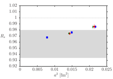
Figure 1: Results for $R_{s}$, the ratio of $B^{*}_{s}$ to $B_{s}$ decay constants (multiplied by the square root of the mass ratio), plotted against the square of the lattice spacing in $\mathrm{fm}^{2}$. Note the magnified $y$-axis scale. The errors on the data points include statistical/fitting errors. Blue filled squares are results on sets with $m_{l}/m_{s}=0.2$, red filled circles sets with $m_{l}/m_{s}=0.1$ and green filled triangles sets with physical $m_{l}$. The grey shaded band gives our physical result including all systematic errors discussed in the text. The black dotted line marks the value 1.0.

From Table 5 and 6 it is immediately clear that the leading order amplitudes, $\Phi^{(0)}$, show a difference between vector and pseudoscalar mesons with the vector result being smaller than the pseudoscalar. This difference is largely down to the ‘hyperfine’ interaction in the NRQCD Hamiltonian (the term with coefficient $c_{4}$ in eq. (2)). The Tables make clear that the impact of this interaction is to lower the ratio of vector to pseudoscalar decay constants. This effect agrees in sign with that seen in an earlier lattice NRQCD analysis of the impact of different relativistic corrections on heavy-light meson decay constants Collins et al. (1997, 1999). It also agrees with early estimates using HQET and QCD sum rules Ball (1994).

From the tables it is also clear that the relativistic current correction matrix element, $\Phi^{(1)}$, has opposite sign for the vector and pseudoscalar cases, being positive for the vector and negative for the pseudoscalar. The impact of these corrections is then to raise the ratio of vector to pseudoscalar decay constants. This sign, and the fact that the pseudoscalar $J^{(1)}$ matrix element is approximately three times that of the vector, agrees with HQET expectations Neubert (1992); Ball (1994) and earlier lattice NRQCD analyses Collins et al. (1997, 1999).

Simply dividing the current correction matrix element, $\Phi^{(1)}$, by $\Phi^{(0)}$ gives naively a relative contribution to the amplitude from the relativistic current corrections of size -(8-10)% for the pseudoscalar and +3% for the vector. This does not take into account the fact that the addition of the relativistic current correction $J^{(1)}$ which appears at tree-level changes the overall renormalisation of the lattice NRQCD current at $\mathcal{O}(\alpha_{s})$ because radiative corrections to $J^{(1)}$ can look like $J^{(0)}$ Monahan et al. (2013). Therefore to determine more accurately the effect of the relativistic current corrections we have to compare the renormalised result with and without the inclusion of the $J^{(1)}$ current correction.

This is done in Table 8 in which we compare the two results for the ratio of $f\sqrt{M}$ for $B^{*}_{s}$ and $B_{s}$. The right-hand column, denoted $R_{s}$, is the full result obtained from eq. (10) using the values of $\delta z$ from Table 7. The values for $\alpha_{s}$ used in that expression are taken in $V$ scheme at the scale $2/a$, where $a$ is the lattice spacing on that ensemble, and are given in Table 1. The column denoted $R_{s}^{\mathrm{L}O}$ gives results using only the leading-order currents and

$$R^{\mathrm{LO}}_{s}=(1+\delta z^{\mathrm{LO}}\cdot\alpha_{s})\frac{\Phi_{B^{*}_{s}}^{(0)}}{\Phi_{B_{s}}^{(0)}}$$ (12)

with $\delta z^{\mathrm{LO}}$ values given in Table 7 and the same values of $\alpha_{s}$. Note the difference between $\delta z^{\mathrm{LO}}$ and $\delta z$. Both coefficients are small, but they have opposite sign. This then compensates to some extent for the effect of the current corrections and means that, comparing $R_{s}$ and $R_{s}^{\mathrm{LO}}$ in Table 8 we see now that the total effect of the current correction terms in the ratio amounts to 7-8%, somewhat less than the naive estimate of 12-15%. There is of course an uncertainty on this estimate coming from missing $\alpha_{s}^{2}$ terms in the renormalisation. A similar procedure would be needed to estimate accurately the effect of the hyperfine term on the ratio $R_{q}$. However, because the hyperfine interaction is embedded in the NRQCD Hamiltonian it is automatically included in the perturbative matching calculation for the NRQCD currents and we do not have the $z$ coefficients without the hyperfine term included. Note that the size of the hyperfine coefficient ($c_{4}$ in eq. (2)) is tested through determination of the mass splitting between vector and pseudoscalar mesons in Dowdall et al. (2012b).

III.2 $f_{B_{s}^{*}}$

Figure 1 plots the full results for $R_{s}$, the ratio of $f\sqrt{M}$ for the $B^{*}_{s}$ and $B_{s}$ mesons, obtained from eq. (10) and given as column 5 of Table 8. Statistical errors in $R_{s}$ are small, less than 0.5%, so we see that the value for the ratio is clearly less than 1 and the dependence on the lattice spacing is small, but clear and unambiguous. To derive a physical result we need to fit this dependence, as discussed in Section II.1, allowing for other systematic uncertainties from lattice QCD.

The key sources of systematic error that need to be allowed for, by inclusion in our fit function, are:

• Matching uncertainties - $\alpha_{s}^{2}$. The missing $\alpha_{s}^{2}$ coefficient in the overall renormalisation factor for the ratio of amplitudes of the NRQCD currents is potentially the largest source of uncertainty here. We can allow for this by simply taking a fractional error which is $\alpha_{s}^{2}\approx 0.1$ times a value for this coefficient. However, the value of $\alpha_{s}^{2}$ changes with the lattice spacing and the coefficient may also depend on $am_{b}$, as the known one-loop coefficient $\delta z$ does, see Table 7. Thus a better estimate is obtained by incorporating a factor to take account of this missing term into the fit. We write the factor as $(1+c\alpha_{s}^{2})$ and take $c$ to have the form $c_{1}\times(1+c_{2}\delta x_{m}+c_{3}\delta x_{m}^{2})$ where $c_{1}$ sets the overall allowed size of the coefficient and the $\delta x_{m}$ terms allow for dependence on $am_{b}$. $\delta x_{m}=(am_{b}-2.7)/1.5$ varies from -0.5 to 0.5 over the range of $am_{b}$ values we use here Dowdall et al. (2012a).

• Matching uncertainties - $\alpha_{s}\Lambda/m_{b}$. We must also allow for missing $\alpha_{s}$ terms that alter the normalisation of the relativistic current corrections within the NRQCD current and/or include the matrix elements of additional current corrections that only appear first at $\mathcal{O}(\alpha_{s}\Lambda/m_{b})$. Such corrections were included in our determination of $f_{B_{s}}$ and $f_{B}$ in Dowdall et al. (2013a) since they are known for the temporal axial current for massless HISQ quarks Monahan et al. (2013). They will be discussed further in Subsection III.5 but here we must include an uncertainty for the fact that they are missing in our ratio. For this we can include an additional term in the factor described above of the form $d\alpha_{s}\Lambda/m_{b}$ where $d$ has an expansion in powers of $\delta x_{m}$ of the same form as $c$ above. Here we can take $\Lambda/m_{b}$ to be 0.08, the size of the relativistic current corrections as determined above.

• Matching uncertainties - $(\Lambda/m_{b})^{2}$. Further current corrections at the next order in the relativistic expansion would appear at $(\Lambda/m_{b})^{2}$. Since we have no information about these we do not include them in the fit but take an additional uncertainty of $(0.1)^{2}$ = 1% (where 0.1 is a suitable power-counting estimate of $\Lambda/m_{b}$) to account for them.

• NRQCD systematics. The improved NRQCD Hamiltonian that we use (eq. (2)) is accurate through $\mathcal{O}(\alpha_{s}\Lambda/m_{b})$ in the context of heavy-light power-counting. Thus the hyperfine interaction that contributes to $R_{s}$ is accurate through this order, which is to a higher order than the matching uncertainties discussed above. Errors from the NRQCD Hamiltonian are then smaller than, and are effectively included in, the matching uncertainties already discussed. Likewise missing terms in the NRQCD Hamiltonian are at even higher order, $\mathcal{O}(1/m_{b}^{3})$ Lepage et al. (1992).

• Discretisation uncertainties. These can come from the gluon action, the HISQ action and the NRQCD action. However, most discretisation uncertainties will cancel between vector and pseudoscalar mesons since the difference between them is a spin-dependent effect and hence suppressed by $\Lambda/m_{b}$. This is clear from Figure 1 which shows very little dependence on $a$. In all three actions discretisation errors appear as even powers of $a$. We therefore include a factor $(1+(\Lambda/m_{b})\sum_{j}e_{j}(\Lambda a)^{2j})$ to allow for these uncertainties in the fit. We take a value 0.2 for $\Lambda/m_{b}$ here to be conservative. For $e_{1}$ we allow for dependence on $am_{b}$ coming from the NRQCD action as discussed in Section II.1 and above for the coefficients $c$ and $d$.

• Tuning uncertainties - valence quark masses. Our valence masses are tuned very accurately (to an uncertainty of 1%) but we allow for effects of mistuning. For the $s$ quark mass these will be negligible since, as we show below, the difference between $R_{s}$ and $R_{l}$ is very small. Mistuning of the $b$ quark mass will affect $R_{s}$ through the hyperfine interaction and the size of the current correction matrix elements, i.e. through a term of the form $(\Lambda/m_{b})\delta m_{b}/m_{b}$. We therefore allow for a term of this form in the factor that includes discretisation effects above. We determine $\delta m_{b}$ from the physical values for $m_{b}$ given on each ensemble in Dowdall et al. (2012a, b) and these are tabulated in Table 1. The largest value of $\delta m_{b}/m_{b}$ is 1.3% on set 4.

• Tuning uncertainties - sea quark masses. Our results include values on ensembles of gluon field configurations at a variety of values of the $u/d$ quark mass in the sea, varying from $0.2m_{s}$ down to the physical point. The $s$ and $c$ quark masses in the sea are well-tuned. Dependence on the sea quark masses is very small, as is clear from Figure 1. We therefore include a simple linear dependence on the sea quark masses, as might be expected from leading-order chiral perturbation theory. This dependence takes the form $g\delta m_{\mathrm{sea}}/(10m_{\mathrm{sea,phys}})$ where the mass-dependent variable is a physical one because we take a mass ratio in which $Z$ factos cancel. We include $u/d$ and $s$ quarks in $m_{\mathrm{sea}}$ and the factor of 10 is a convenient way to introduce the chiral scale of 1 GeV expected from chiral perturbation theory. $\delta m_{\mathrm{sea}}=(2m_{l}+m_{s})-(2m_{l,\mathrm{phys}}+m_{s,\mathrm{phys}})$ and is obtained using values for $m_{s,\mathrm{phys}}$ given in Dowdall et al. (2012a). We take $m_{l,\mathrm{phys}}/m_{s,\mathrm{phys}}$ = 1/27.4 Bazavov et al. (2014). Values for $\delta x_{\mathrm{sea}}\equiv\delta m_{\mathrm{sea}}/m_{\mathrm{sea,phys}}$ on each ensemble are given in Table 1.

• Uncertainties in the value of the lattice spacing. Since we are determining a dimensionless ratio of decay constants, uncertainties in the value of the lattice spacing only enter indirectly through the uncertainty in tuning the quark masses. As discussed above the tuning of $m_{b}$ affects the size of the relativistic correction terms that affect the vector/pseudoscalar ratio. We have a 1% uncertainty in our lattice spacing values, largely correlated between the ensembles and so we add an additional overall uncertainty of $0.2\times 0.01$ = 0.2% to allow for this. The factor of 0.2 is a conservative estimate for the size of relativistic corrections.

Putting the features above together we arrive at a fit form for $R_{s}$ as a function of $a$ and quark masses as:

$$R_{s}(a,m) = R_{s,\mathrm{phys}}\times F_{1}(a,m)/F_{2}(\alpha_{s})$$ (13)

$$F_{2}(\alpha_{s}) = (1+c\alpha_{s}^{2}+0.08d\alpha_{s})$$

$$F_{1}(a,m) = 1+0.2\sum_{j=1}^{3}e_{j}(\Lambda a)^{2j}$$

$$+ 0.2f\frac{\delta m_{b}}{m_{b,\mathrm{phys}}}+g\frac{\delta m_{\mathrm{s}ea}}{10m_{\mathrm{sea,phys}}}$$

$$c = c_{1}\times(1+c_{2}\delta x_{m}+c_{3}(\delta x_{m})^{2})$$

$$d = d_{1}\times(1+d_{2}\delta x_{m}+d_{3}(\delta x_{m})^{2})$$

$$e_{1} = e_{11}\times(1+e_{12}\delta x_{m}+e_{13}(\delta x_{m})^{2})$$

In dividing by $F_{2}$ we follow the convention that we used at $\mathcal{O}(\alpha_{s})$ in eq. (10) of writing the renormalisation as a multiplicative factor. Thus if $F_{2}$ were instead known, rather than fitted, the raw results would be multiplied by this correction factor along with the factor at $\mathcal{O}(\alpha_{s})$. We use a Bayesian fitting approach Lepage et al. (2002) to implement the fit function of eq. (13). Priors on all of the coefficients are taken as 0.0(1.0) except for $c_{1}$, which is taken as 0.0(0.2). This allows for an $\alpha_{s}^{2}$ coefficient in the overall renormalisation factor that is twice as large as the largest seen at $\mathcal{O}(\alpha_{s})$ (see $\delta z$ values in Table 7). The prior on the physical value, $R_{s,\mathrm{phys}}$, is taken as 1.0(0.2).

Applying this fit function to our results gives a $\chi^{2}/{\mathrm{dof}}=0.13$ and a physical result for $R_{s}$ of 0.957(23), when we include the uncertainty from missing higher order current corrections and the lattice spacing. The error budget from the fit is laid out in Table 9. As expected the uncertainty is dominated by that from current matching, although the fit has constrained this uncertainty to be a bit smaller than the naive expectation. The physical value, along with the total error, is plotted as a grey band on Figure 1. $R_{s}$ is the ratio of decay constants multiplied by the square root of the meson masses. Our earlier results Dowdall et al. (2012b) showed that the vector and pseudoscalar meson masses calculated here agree with experiment. We can therefore convert our value of $R_{s}$ to a ratio for the decay constants using the square root of the experimental ratio of the meson masses of 1.0045(2) Olive et al. (2014). We obtain:

$$\frac{f_{B^{*}_{s}}}{f_{B_{s}}}=0.953(23).$$ (14)

This is 2$\sigma$ below 1.

Table 9: Full error budget for the various ratios of vector to pseudoscalar decay constants that we calculate here, giving each error as a percentage of the final answer, following the discussion of uncertainties in the text. The effects of finite volume and missing electromagnetism are expected to be negligible.

	$R_{s}$	$R_{l}/R_{s}$	$R_{c}/R_{s}$
stats/fitting/scale	0.6	0.8	0.7
current matching	1.9	1.0	0.8
$(\Lambda/m_{b})^{2}$ currents	1.0	0.2	0.5
$a$-dependence	0.9	0.1	0.15
$m_{\mathrm{sea}}$-dependence	0.05	0.2	0.1
$m_{b}$ tuning	0.4	0.03	0.1
Total	2.4	1.3	1.2

III.3 $f_{B^{*}}$

To analyse the corresponding ratio, $R_{l}$, for the $B/B^{*}$ it is convenient to take the ratio to $R_{s}$. Table 6 gives our results for the $B$ and $B^{*}$ amplitudes and Table 8 gives the ratio of the sum of amplitudes for $J^{(0)}$ and $J^{(1)}$ for vector and pseudoscalar. These results include the correlations between the vector and pseudoscalar meson correlators from the simultaneous fit. The results for $B^{*}_{l}/B_{l}$ are very similar, not surprisingly, to those for $B_{s}$ and $B^{*}_{s}$. The statistical errors are significantly larger, however, as is expected when the light quark mass is reduced Davies et al. (2010a). The renormalisation factor (eq. (10)) for $R_{l}$ is the same as that for $R_{s}$ (since mass effects for light quarks are negligible in the matching) and so the renormalisation cancels in the ratio $R_{l}/R_{s}$. We can therefore simply determine $R_{l}/R_{s}$ from the ratio of the first two columns in Table 8:

$$\frac{R_{l}}{R_{s}}=\left(\frac{\Phi^{(0)}_{B^{*}_{l}}+\Phi^{(1)}_{B^{*}_{l}}}{\Phi^{(0)}_{B_{l}}+\Phi^{(1)}_{B_{l}}}\right)\left(\frac{\Phi^{(0)}_{B_{s}}+\Phi^{(1)}_{B_{s}}}{\Phi^{(0)}_{B^{*}_{s}}+\Phi^{(1)}_{B^{*}_{s}}}\right).$$ (15)

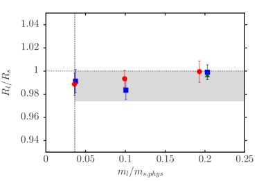
Figure 2: Results for $R_{l}/R_{s}$, the SU(3)-breaking ratio of the ratio of vector to pseudoscalar decay constants (multiplied by the square root of the mass) plotted against the light quark mass (the average of $u$ and $d$) in units of the physical $s$ quark mass. The filled blue squares gives results on very coarse lattices, red filled circles, on coarse and filled green triangles, on fine. The errors on the data points include statistical/fitting errors. The grey shaded band gives the physical result including all systematic errors discussed in the text. The black dashed line shows the physical value of $m_{l}/m_{s,phys}$ and the blue dotted line indicates the value 1.0.

Figure 2 shows our results for $R_{l}/R_{s}$ on each ensemble, plotted against the light quark mass in units of the physical $s$ quark mass taken from Dowdall et al. (2012a). The results are very close to the value 1.0, but show a small downward trend as the light quark mass falls towards its physical value. There is no significant dependence on the lattice spacing.

To fit the dependence of $R_{l}/R_{s}$ and extract a physical result, we use much of the same fit function as that given for $R_{s}$ in eq. (13). The two key differences are that the overall renormalisation factor now cancels, so that we can drop the factor $c\alpha_{s}^{2}$ from $F_{2}$, and that we now want to include a fitted dependence on $m_{l}$. We can also use the known similarity of $B_{l}$ and $B_{s}$ to constrain the fit further. For example, we know that decay constants for heavy-light and heavy-strange mesons differ by about 20% Dowdall et al. (2013a); Follana et al. (2008). This is in fact a very strong result, still true even when the light/strange quark is accompanied by a light or strange quark (see, for example, Dowdall et al. (2013b) for $\pi$, $K$ and $\eta_{s}$ results). The $d\alpha_{s}$ term in eq. (13) takes account of missing radiative corrections to the sub-leading currents, $J^{(1)}$. We retain that term here but multiply its coefficient by 0.2 to allow for strange/light differences in the matrix element for $J^{(1)}$. We reduce the coefficient 0.2 (allowed for the size of $\Lambda/m_{b}$) in front of discretisation errors and $m_{b}$ tuning terms by a further factor of 0.2 for the same reason. Finally, we include an additional term in the fit to allow for dependence on the light valence mass, since we have results for a variety of $m_{l}$ values. For this we include a term in $F_{1}$ of the form $h(m_{l}/(10m_{s,\mathrm{phys}}))$. The factor of 10 once again is used to convert $m_{s}$ into the chiral scale of 1 GeV. The prior on $h$ is taken as 0.0(1.0). Since this term is already largely covered by including a term to allow for sea quark mass dependence, it has very little impact.

The fit has a $\chi^{2}/{\mathrm{dof}}$ of 0.23 and gives a physical result:

$$\frac{R_{l}}{R_{s}}=0.987(13).$$ (16)

Since $R_{l}/R_{s}$ measures both SU(3)-breaking and spin-breaking effects in heavy-light meson decay constants we expect a result very close to 1.0. Our value is consistent with 1, but enables us to constrain any difference from 1.0 to a few percent. We will return to this in section III.4 when comparing to results for $B_{c}$ mesons. A full error budget for $R_{l}/R_{s}$ is given in Table 9.

Combining our result for $R_{l}/R_{s}$ with our earlier result for $R_{s}$ gives $R_{l}=0.945(26)$. Combining with the experimental value for the square root of the ratio of the meson masses, 1.0043 Olive et al. (2014), we obtain

$$\frac{f_{B^{*}_{l}}}{f_{B_{l}}}=0.941(26)$$ (17)

which is more than $2\sigma$ below 1.

III.4 $f_{B_{c}}$ and $f_{B_{c}^{*}}$

Table 10: Amplitudes for $J^{(0)}$ and $J^{(1)}$ for temporal axial and vector currents between the vacuum and the $B_{c}$ and $B_{c}^{*}$ mesons respectively, extracted from correlator fits and multiplied by $\sqrt{2}$ in accordance with eq. (9). Results are in lattice units and the errors given are statistical/fit errors only. The ground-state energies determined from the fits agree with those given in Dowdall et al. (2012b) and we do not repeat them here.

Set	$a^{3/2}\Phi_{B_{c}}^{(0)}$	$a^{3/2}\Phi_{B_{c}}^{(1)}$	$a^{3/2}\Phi_{B^{*}_{c}}^{(0)}$	$a^{3/2}\Phi_{B^{*}_{c}}^{(1)}$
1	0.83048(86)	-0.04792(5)	0.8022(11)	0.01541(3)
2	0.82001(45)	-0.04779(3)	0.7904(6)	0.01532(2)
4	0.58564(17)	-0.04068(2)	0.54496(22)	0.01267(1)
5	0.57350(11)	-0.04055(1)	0.53195(14)	0.01260(1)
7	0.36166(9)	-0.03158(1)	0.31990(11)	0.00941(1)

Table 11: Coefficients $z_{A_{0},c}$ and $z_{1}$, $z_{2}$ used in the matching factors to determine the decay constant for the $B_{c}$ meson (eq. (III.4)). $z_{A_{0},c}$ is constructed from results given for the appropriate NRQCD bare masses and massive HISQ quarks with the appropriate values of $m_{c}a$ in Monahan et al. (2013) as $z_{c}=\eta_{0}-\tau_{10}$. $z_{1}$ and $z_{2}$ are results for massless HISQ quarks Dowdall et al. (2013a); Monahan et al. (2013). The values of $\alpha_{s}$ used with these $z$ coefficients are given in Table 1.

Set	$z_{A_{0},c}$	$z_{1}$	$z_{2}$
1	-0.111(5)	0.024(3)	-1.108(4)
2	-0.105(5)	0.024(3)	-1.083(4)
4	-0.046(5)	0.007(3)	-0.698(4)
5	-0.041(5)	0.007(3)	-0.690(4)
7	-0.034(5)	-0.031(4)	-0.325(4)

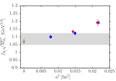
Figure 3: Results for the decay constant of the $B_{c}$ meson (multiplied by the square root of its mass) obtained with NRQCD $b$ quarks and HISQ $c$ quarks for ensembles at different values of the lattice spacing as described in the text. The errors on the points include uncertainties in the value of the lattice spacing and statistical/fitting errors. Blue filled squares give results at sea light quark mass $m_{l}/m_{s}=0.2$ and red filled squares at $m_{l}/m_{s}=0.1$. The grey shaded band gives the physical result including all systematic errors discussed in the text. For comparison we include as the green burst the physical result obtained from using the HISQ formalism for both $b$ and $c$ quarks McNeile et al. (2012a).

$B_{c}$ and $B^{*}_{c}$ meson correlation functions are calculated from NRQCD $b$ and HISQ $c$ propagators in exactly the same way as those described for NRQCD $b$ and HISQ $s$ or $l$ propagators in subsection III.1. We do not include the full set of ensembles used for the lighter HISQ quark mass calculations since experience has shown very little sea quark mass dependence for heavy meson correlators that do not include valence light quarks Gregory et al. (2011); Dowdall et al. (2012b). We thus include ensembles at two different values of the sea $u/d$ quark mass for very coarse and coarse sets rather than three. The meson correlation functions are fit simultaneously so that correlations between them can be included in the determination of the ratio of amplitudes needed for the ratio of decay constants.

The results for the matrix elements, $\Phi$, of the leading, $J^{(0)}$, and subleading, $J^{(1)}$, pieces of the temporal axial and spatial vector currents are given in Table 10. We first discuss combining the results for the temporal axial current into a value for the decay constant of the pseudoscalar $B_{c}$ meson. We will use a formula Dowdall et al. (2013a) which is somewhat more accurate than that used in eq. (9):

$$f_{B_{c}}\sqrt{M_{B_{c}}}=(1+z_{A_{0},c}\alpha_{s}) \times \left(\Phi_{B_{c}}^{(0)}+\Phi_{B_{c}}^{(1)}\right.$$

$$+ \left.z_{1}\alpha_{s}\Phi_{B_{c}}^{(1)}+z_{2}\alpha_{s}\Phi_{B_{c}}^{(2)}\right).$$

$z_{1}\alpha_{s}$ is an additional radiative correction to the sub-leading current $J^{(1)}$. $z_{2}\alpha_{s}$ multiplies an additional sub-leading current which has the same matrix element as $J^{(1)}$ and so does not need to be separately calculated. The $z$ coefficients now have to be calculated for massive HISQ quarks with a mass in lattice units corresponding to our values for $am_{c}$ on the different ensembles. This has been done for $z_{A_{0},c}$ and the values are given in Table 11. They differ slightly from those for massless HISQ quarks in Table 7 but are still very much less than 1. The $z_{1}$ and $z_{2}$ coefficients have only been calculated for massless HISQ quarks and these are also given in Table 11. There is then a systematic error in our formula of eq. (III.4) as a result of using the massless $z_{1}$ and $z_{2}$ coefficients and we will allow for that in our error budget along with systematic errors from unknown higher order terms in the overall renormalisation factor.

The results obtained from applying eq. (III.4) are plotted in Figure 3 as a function of lattice spacing. We see, as expected, very little change between ensembles with similar lattice spacings but different sea $u/d$ quark masses. To determine a physical value for the decay constant we fit the results to a functional form that includes allowance for systematic errors in the lattice QCD calculation.

The systematic errors have the same sources as those discussed for $R_{s}$ in section III.1 and we will use the same fit form as that given in eq. (13) and we reproduce that below as eq. (III.4) with the modifications appropriate here. As in section III.1, the major source of uncertainty here comes from missing higher order terms in the matching of the NRQCD-HISQ current to continuum QCD. This is taken account of in eq. (III.4), as before, by the term $F_{2}(\alpha_{s})$ which includes an $\alpha_{s}^{2}$ term with coefficient $c$ in the overall renormalisation factor and a term with coefficient $d$ that allows for systematic errors in the $\alpha_{s}$ corrections to the $J^{(1)}$ current contribution included in eq. (III.4) from the fact that $z_{1}$ and $z_{2}$ are taken for massless HISQ quarks. Given the values we have for $z_{A_{0},c}$ and the dependence on $am_{c}$ seen in that coefficient, we do not expect coefficients $c$ and $d$ to be large and we take priors on their fit values of 0.0(0.2).

From Fig. 3 we see significant lattice spacing dependence in the results and we must allow both for regular lattice spacing dependence and that coming from the NRQCD action. This dependence is included in factor $F_{1}$. The regular lattice spacing coming the HISQ action can have a scale set by $m_{c}$ in this case and we expect that to dominate. We take $m_{c}$ to be 1 GeV here. The analysis of discretisation errors for $c$ quarks in the HISQ action Follana et al. (2007) shows that the dependence comes from terms suppressed by powers of the velocity of the $c$ quark. Since $v_{c}^{2}\approx 0.5$ in a $B_{c}$ Gregory et al. (2010) we include a factor of 0.5 in front of the terms allowing for discretisation errors. We must also allow for dependence on the $u/d$ quark mass in the sea, as before, and for mistuning of the $b$ quark mass. For mistuning of the $b$ quark mass we allow a conservative factor of 0.3 based on the variation in decay constants between heavyonium mesons (see Fig. 8).

Our fit function is:

$$f_{B_{c}}\sqrt{M_{B_{c}}}(a,m) = \left(f_{B_{c}}\sqrt{M_{B_{c}}}\right)_{\mathrm{phys}}$$

$$\times F_{1}(a,m)/F_{2}(\alpha_{s});$$

$$F_{2}(\alpha_{s}) = (1+c\alpha_{s}^{2}+0.08d\alpha_{s})$$

$$F_{1}(a,m) = 1+0.5\sum_{j}e_{j}(m_{c}a)^{2j}$$

$$+ 0.3f\frac{\delta m_{b}}{m_{b,\mathrm{phys}}}+g\frac{\delta m_{\mathrm{s}ea}}{10m_{\mathrm{sea,phys}}}$$

$$c = c_{1}\times(1+c_{2}\delta x_{m}+c_{3}(\delta x_{m})^{2})$$

$$d = d_{1}\times(1+d_{2}\delta x_{m}+d_{3}(\delta x_{m})^{2})$$

$$e_{1} = e_{11}\times(1+e_{12}\delta x_{m}+e_{13}(\delta x_{m})^{2})$$

We take prior values on all coefficients to be 0.0(1.0) except for the physical value on which we take 1.0(2), $c$ and $d$, on which we take 0.0(2) and $e_{1}$ on which we take 0.0(3) (since it is $\mathcal{O}(\alpha_{s})$). The error on the plotted values in Figure 3 is dominated by the uncertainty in the value of the lattice spacing (given in Table 1). In doing the fit we allow for half of this error to be correlated between ensembles (since it comes from systematic uncertainties from the NRQCD calculation used to fix the lattice spacing Dowdall et al. (2012a)) and half to be uncorrelated.

The fit gives a $\chi^{2}/\mathrm{dof}$ of 0.11 and a physical value for $f\sqrt{M}$ for the $B_{c}$ of 1.087(37) $(\mathrm{GeV})^{3/2}$. The 3.4% uncertainty is split between 1.2% from matching and 3.2% from other sources, dominated by lattice spacing uncertainties and discretisation errors. We have checked that missing out $z_{1}$ and $z_{2}$ from eq. (III.4) and allowing a larger prior of 0.0(1.0) on the coefficient $d$ in eq. (III.4) gives a physical result with almost the same central value and uncertainty.

Our physical result is plotted as a grey band in Figure 3. It agrees very well with our result of 1.070(15) ${\mathrm{GeV}}^{3/2}$ McNeile et al. (2012a) based on using the HISQ action for a heavy quark combined with a HISQ $c$ quark and working at a range of heavy quark masses between $c$ and $b$ on lattices with a range of lattice spacings from 0.15 fm down to 0.045 fm. The HISQ-HISQ result has an uncertainty which is a factor of 2 smaller than the NRQCD-HISQ result we give here. This is because the HISQ-HISQ current is absolutely normalised in the calculation of pseudoscalar decay constants and the calculation is done over a wider range of values of the lattice spacing for better control of discretisation errors. Good agreement between the HISQ-HISQ result and NRQCD-HISQ result was already seen for the $B_{s}$ in McNeile et al. (2012b); Dowdall et al. (2013a) and this further test increases our confidence in our handling of lattice QCD errors. In particular it is an important test of our normalisation of improved NRQCD-HISQ currents that are also in use for semileptonic decay rate calculations underway on these gluon field configurations.

Using the experimental value of the $B_{c}$ meson mass of 6.276(1) GeV Aaij et al. (2013) we can convert our value for $f\sqrt{M}$ into a result for the decay constant:

$$f_{B_{c}}=0.434(15)\mathrm{GeV}.$$ (20)

Again this agrees with our earlier result using HISQ quarks of 0.427(6) GeV McNeile et al. (2012a).

Table 12: Column 2 gives the Coefficient $z_{V_{i},c}$ needed for the one-loop renormalisation factor for the vector decay constant $B^{*}_{c}$. $z_{V_{i},c}$ is constructed from results given for the appropriate NRQCD bare masses and massive HISQ quarks with the appropriate values of $m_{c}a$ in Monahan et al. (2013) as $z_{c}=\eta_{0}-\tau_{10}$. Column 3 gives $\delta z_{c}$, which is the difference between $z_{V_{i},c}$ and $z_{A_{0},c}$ from Table 11. Column 4 gives the difference between $\delta z_{c}$ and the corresponding value $\delta z$ for massless HISQ quarks (from Table 7). The values of $\alpha_{s}$ used with these $z$ coefficients are given in Table 1. Column 5 gives the unrenormalised ratio of vector to pseudoscalar amplitudes (see text) determined from the simultaneous fit to $B^{*}_{c}$ and $B_{c}$ meson correlators. Results from columns 4 and 5 are used in the determination of $R_{c}/R_{s}$.

Set	$z_{V_{i},c}$	$\delta z_{c}$	$\delta z_{c}-\delta z$	$R_{c}^{\mathrm{unren.}}$
1	-0.166(5)	-0.055(7)	0.047(8)	1.0447(14)
2	-0.160(5)	-0.055(7)	0.044(8)	1.0434(8)
4	-0.073(5)	-0.027(7)	0.052(8)	1.02324(27)
5	-0.068(5)	-0.027(7)	0.046(8)	1.02175(17)
7	-0.013(5)	0.021(7)	0.058(8)	0.99766(22)

Figure 4: Results for the ratio of $R_{c}$ to $R_{s}$ plotted against the square of the lattice spacing. $R_{c}$ is the ratio of vector to pseudoscalar decay constants ($f\sqrt{M}$) for the $B^{*}_{c}$ and $B_{c}$ and $R_{s}$ is the corresponding ratio for the $B^{*}_{s}/B_{s}$. Filled blue squares are results on ensembles with $m_{l}/m_{s}=0.2$ and filled red circles results on ensembles with $m_{l}/m_{s}=0.1$. The errors on the points are statistical errors only (including those from $(\delta z_{c}-\delta z)$). The grey shaded band gives the physical result including all systematic errors as discussed in the text. The black dashed line marks the value 1.0.

The vector to pseudoscalar decay constant ratio, $R_{c}$, is obtained in an analogous way to that for the $B_{s}$ and $B^{*}_{s}$ mesons described in Section III.1. The formula we use is that given in eq. 10, in which $z_{A_{0}}$ and $z_{V_{i}}$ are the coefficients calculated for temporal axial and spatial vector currents respectively using HISQ quark mass values appropriate to $c$ quarks. Values for $z_{A_{0},c}$ are given in Table 11 and values for $z_{V_{i},c}$ are given in Table 12. Table 12 also gives $\delta z_{c}$, the difference between the two, which is needed for the decay constant ratio in eq. 10. Note that we are now neglecting radiative corrections to the current correction $J^{(1)}$ (i.e. the terms with coefficients $z_{1}$ and $z_{2}$ in eq. (III.4)) since we do not have these terms for the vector current.

Table 10 gives the results for the amplitudes that we need to construct the decay constants and their ratio. We see that the qualitative features of the results are the same i.e. that the amplitude of the leading order current is smaller for the vector than for the pseudoscalar meson, lowering the vector to pseudoscalar decay constant ratio, whereas the current correction contributions have opposite effect. The impact of the current corrections is a few percent less than in the $B_{s}$ case but varies more strongly with lattice spacing.

In a similar approach to that used for $R_{l}$ in Section III.1 we will study $R_{c}$ through its ratio with $R_{s}$. In this case the renormalisation factor does not cancel completely at $\mathcal{O}(\alpha_{s})$ since $\delta z_{c}$ is not equal to $\delta z$. Instead we have a renormalisation factor for $R_{c}/R_{s}$ which is $(1+[\delta z_{c}-\delta z]\alpha_{s})$, i.e. we can write:

$$\frac{R_{c}}{R_{s}}=(1+[\delta z_{c}-\delta z]\alpha_{s})\left(\frac{\Phi^{(0)}_{B^{*}_{c}}+\Phi^{(1)}_{B^{*}_{c}}}{\Phi^{(0)}_{B_{c}}+\Phi^{(1)}_{B_{c}}}\right)\left(\frac{\Phi^{(0)}_{B_{s}}+\Phi^{(1)}_{B_{s}}}{\Phi^{(0)}_{B^{*}_{s}}+\Phi^{(1)}_{B^{*}_{s}}}\right)$$ (21)

Values of $(\delta z_{c}-\delta z)$ are given in Table 12. We see that these are small and independent of the value of $am_{b}$ within statistical uncertainties. Since the dependence on $am_{b}$ comes from the NRQCD action it is not surprising to find some cancellation between these two cases. The remaining small renormalisation then reflects the fact that the $c$ quark mass is not zero (i.e. $m_{c}/m_{b}\neq 0$). Table 12 gives in the final column results for the appropriate ratio of sums of amplitudes needed in eq. (21), i.e. $R^{\mathrm{unren.}}_{c}$. This can be combined with $R^{\mathrm{unren.}}_{s}$ from Table 5 and the small renormalisation applied to form $R_{c}/R_{s}$.

Figure 4 gives results for the ratio of $R_{c}$ to $R_{s}$ from eq. (21) as a function of lattice spacing. We see that the results are independent of lattice spacing and sea quark mass. Importantly the values obtained are all significantly larger than 1.0, showing that the vector to pseudoscalar decay constant ratio is sensitive to the mass of the light quark combined with the $b$. Half of the difference from 1.0 comes from the raw amplitudes and the other half from the renormalisation factor in eq. (21).

In fitting this ratio as a function of lattice spacing to obtain a physical result we will use the same fit form as that used in subsection III.1, eq. (13). The only change in form that we make is to remove $am_{b}$ dependence from the coefficient of unknown $\alpha_{s}^{2}$ renormalisation terms in the factor $F_{2}$ assuming they follow the same form as discussed above for the $\mathcal{O}(\alpha_{s})$ term. We take the radiative correction terms for the $J^{(1)}$ currents in $F_{2}$ to have the same form as in eq. (13) but allow for cancellation between $R_{c}$ and $R_{s}$ by giving that term coefficient 0.03 rather than 0.08. For the discretisation errors and $m_{b}$ tuning error terms in $F_{1}$ we likewise allow for cancellation between $R_{c}$ and $R_{s}$ by giving these terms coefficient 0.1 rather than 0.2.

The fit to our results gives $\chi^{2}/{\mathrm{dof}}$ of 0.1 and a physical result of

$$\frac{R_{c}}{R_{s}}=1.037(12)$$ (22)

where we have allowed a 0.5% uncertainty from missing higher-order relativistic current corrections. This value is $3\sigma$ greater than 1.0 giving a clear indication that $R_{q}$ increases as the mass of the quark $q$ increases. This is consistent with what was found (with much lower significance) in Section III.1 for $q=l$ and $s$. Our physical result for $R_{c}/R_{s}$ is plotted as the grey band in Figure 4. A full error budget for $R_{c}/R_{s}$ is given in Table 9.

Using our earlier value for $R_{s}$ of 0.957(23) we obtain $R_{c}$ = 0.992(27). We convert $R_{c}$ into a ratio of the decay constants of the $B^{*}_{c}$ and $B_{c}$ mesons by dividing by the square root of the ratio of the masses. For this we use the experimental value for the $B_{c}$ mass of 6.276(1) GeV Aaij et al. (2013) and our lattice QCD result for the mass difference between $B^{*}_{c}$ and $B_{c}$ of 54(3) MeV Dowdall et al. (2012b). This gives a mass ratio for $B^{*}_{c}$ to $B_{c}$ of 1.0086(5). We then obtain

$$\frac{f_{B^{*}_{c}}}{f_{B_{c}}}=0.988(27).$$ (23)

III.5 Heavy Quark Mass Dependence

Table 13: The coefficients $c_{1}$, $c_{5}$, $c_{4}$ used in the NRQCD action (eq. (2)) for values of the heavy quark mass in lattice units given in column 2. $c_{6}$ is equal to $c_{1}$ and $c_{2}$ and $c_{3}$ are set to 1.0. Amplitudes for $J^{(0)}$ and $J^{(1)}$ for temporal axial and vector currents between the vacuum and heavy pseudoscalar and vector mesons respectively, made from a heavy NRQCD quark and a HISQ $s$ quark and denoted $H_{s}$ and $H^{*}_{s}$. The different heavy quark masses in lattice units used on sets 1 and 4 are given in column 2. Results are in lattice units and the errors given are statistical/fit errors only.

Set	$am_{h}$	$c_{1}$	$c_{5}$	$c_{4}$	$z_{1}$	$z_{2}$	$a^{3/2}\Phi_{H_{s}}^{(0)}$	$a^{3/2}\Phi_{H_{s}}^{(1)}$	$a^{3/2}\Phi_{H^{*}_{s}}^{(0)}$	$a^{3/2}\Phi_{H^{*}_{s}}^{(1)}$	$R_{s}$
1	1.91	1.29	1.18	1.19	-0.031(4)	-0.325(4)	0.3401(6)	-0.04274(10)	0.2958(14)	0.01273(8)	1.0242(43)
	2.66	1.36	1.19	1.21	0.007(3)	-0.698(4)	0.3600(8)	-0.03430(9)	0.3233(16)	0.01052(7)	0.9969(41)
4	1.91	1.26	1.15	1.18	-0.031(4)	-0.325(4)	0.2602(4)	-0.02958(6)	0.2237(6)	0.00865(3)	0.9956(21)
	3.297	1.31	1.17	1.21	0.024(3)	-1.108(4)	0.2802(7)	-0.01997(6)	0.2534(8)	0.00611(2)	0.9657(21)

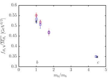
Figure 5: Results for the decay constant of the pseudoscalar heavy-strange meson $H_{s}$ multiplied by the square root of its mass as a function of the heavy quark mass in units of the physical $b$ quark mass. Open red circles are results on set 1 ensembles from improved NRQCD heavy quarks combined with HISQ $s$ quarks (from Tables 5 and 13). The open blue squares are results from $a=$ 0.044 fm lattices using the HISQ formalism for both $b$ and $s$ McNeile et al. (2012b). The solid error bars on both sets of points include statistics and the (correlated) uncertainty in the value of the lattice spacing. The dotted error bars on the NRQCD points include in addition an estimate of NRQCD systematic errors Dowdall et al. (2013a). The black bursts are the final physical values for the $D_{s}$ and $B_{s}$ Davies et al. (2010a); Dowdall et al. (2013a).

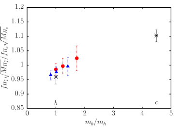
Figure 6: Results for the ratio of vector to pseudoscalar decay constants for heavy-strange mesons made with a range of heavy quark masses, $m_{h}$, as a function of the heavy quark mass in units of $m_{b}$. Filled red circles give results from very coarse set 1, and filled blue triangles from coarse set 4, for NRQCD heavy quarks (Tables 8 and 13). Dotted error bars include an estimate of NRQCD systematic errors. Black bursts indicate the physical result for $B^{*}_{s}/B_{s}$ mesons from this paper and for $D^{*}_{s}/D_{s}$ mesons using HISQ $c$ and $s$ quarks from Donald et al. (2014b).

In this subsection we give results for calculations that use NRQCD quarks with masses lighter than that of the $b$ in order to study the heavy-quark mass dependence of decay constants and their ratios and make a link between $b$ and $c$. Using the HISQ action we have previously mapped out the dependence of pseudoscalar decay constants and quark masses McNeile et al. (2010); McNeile et al. (2012b, a); Chakraborty et al. (2014) in this region in some detail, and we will be able to compare to these results.

The HISQ action has the smallest discretisation errors of any quark action in current use, since it removes tree-level $a^{2}$ errors and has no odd powers of $a$ appearing. It is therefore a very good action for $c$ physics Follana et al. (2007); Davies et al. (2010a); Donald et al. (2012). Raising the mass from that of $c$ requires fine lattices to keep masses in lattice units below $ma=1$, where, naively, it might be expected that discretisation errors would become large. It is possible to reach the $b$ on ‘ultrafine’ lattices with a lattice spacing as small as $a=0.045$ fm. This has given accurate results for $m_{b}$, $f_{B_{s}}$ and $f_{B_{c}}$ McNeile et al. (2010); McNeile et al. (2012b, a) because we can use operators that are absolutely normalised.

For NRQCD the issues are complementary ones. In this case we have systematic control of a non-relativistic effective theory. Discretisation errors are much smaller, having a scale set by internal momenta rather than the quark mass. In this case naive arguments suggest that we need $ma>1$ to control coefficients of relativistic correction operators, for high precision. In fact for $b$ quarks on the ensembles we use here, with lattice spacing values ranging from 0.15 fm down to 0.09 fm, values of $ma$ are well above 1 and there is significant headroom to reduce the mass, particularly on the coarser lattices. Since the ratio of $c$ to $b$ quark mass is 4.5 McNeile et al. (2010), we cannot reach the $c$ quark mass with $ma>1$ even on the very coarse lattices. However, it is still of interest to vary the mass and compare the mass-dependence using NRQCD heavy quarks to that obtained from a completely different perspective, in terms of systematic errors, using HISQ quarks.

We have already shown that using HISQ $b$ quarks and NRQCD $b$ quarks gives results in agreement for the decay constant of the $B_{s}$ McNeile et al. (2012b); Dowdall et al. (2013a) and the $B_{c}$ ( McNeile et al. (2012a) and subsection III.4). Here we will illustrate how well this agreement continues to lighter masses.

We work on one ensemble each from the very coarse (set 1) and coarse (set 4) lattices. We will focus on results using $s$ HISQ quarks where, as we have seen, dependence on the sea $u/d$ mass is negligible. It is most convenient to use the same values of $am_{b}$ as those used before on the finer lattices, since then the coefficients of the radiative corrections to terms in the NRQCD Hamiltonian are already known. We simply have to change the value of $\alpha_{s}$ multiplying them on the coarser lattices. In Table 13 we give the coefficients that we use for heavy quark masses $am_{h}=1.91$ and 2.66 on very coarse set 1 and for $am_{h}=1.91$ and 3.297 on coarse set 4. On very coarse set 1 the lightest $am_{h}$ then corresponds to 1.91/3.297= 0.58 times $m_{b}$. On coarse set 4 the mass 3.297 is higher than $m_{b}$ (since there $am_{b}=2.66$, see Table 1), but $am=1.91$ corresponds to 0.72 times $m_{b}$. The coefficients are calculated by combining the one-loop coefficients at the appropriate $am_{b}$ values given in Dowdall et al. (2012a); Hammant et al. (2011) with the appropriate $\alpha_{s}$ value (also given in Dowdall et al. (2012a)) for that lattice spacing. These coefficients are then used in the NRQCD action (eq. (2)) along with relevant tadpole-improvement factors given in Table 1 for that ensemble.

We again use a local and two smeared sources for the NRQCD propagators, with smearing radii as given in Table 1. We combine the NRQCD propagators with those for the HISQ $s$ quarks on each ensemble. Table 13 gives results for the amplitudes for the leading-order and relativistic correction currents for the heavy-strange pseudoscalar meson ($H_{s}$) and vector meson ($H^{*}_{s}$). These are obtained from simultaneous fits to the vector and pseudoscalar meson correlators as described in subsection II.3.

To determine the pseudoscalar decay constant, $f_{H_{s}}$, we are able to use a more accurate formula than the one given in eq. (9), because additional current corrections coefficients are available in this case (only). We can use the formula accurate through $\alpha_{s}\Lambda/m_{h}$ given in Dowdall et al. (2013a):

$$f_{H}\sqrt{M_{H}}=(1+z_{A_{0}}\alpha_{s}) \times \left(\Phi_{A_{0}}^{(0)}+\Phi_{A_{0}}^{(1)}\right.$$

$$+ \left.z_{1}\alpha_{s}\Phi_{A_{0}}^{(1)}+z_{2}\alpha_{s}\Phi_{A_{0}}^{(2)}\right).$$

$z_{1}\alpha_{s}$ is an additional radiative correction to the sub-leading current $J^{(1)}$. $z_{2}\alpha_{s}$ multiplies an additional sub-leading current which has the same matrix element as $J^{(1)}$ and so does not need to be separately calculated. The coefficients $z_{1}$ and $z_{2}$ are given for the masses we use in Table 13. The $z_{A_{0}}$ values are in Table 7 and $\alpha_{s}$ values in Table 1.

Figure 5 shows results for $f_{H_{s}}\sqrt{M_{H_{s}}}$ as a function of inverse heavy quark mass in units of the physical $b$ quark mass. The results for set 1 are shown as open red circles including the value at the $b$ quark mass ($am_{b}=3.297$) from Table 5 as well as the results for lighter heavy quark masses from Table 13. The solid error bar is the dominant error in the raw results coming from the uncertainty in the lattice spacing. The dotted error bar includes an estimate of systematic errors from NRQCD coming from missing $\alpha_{s}^{2}$ renormalisation and $(\Lambda/m_{h})^{2}$ current corrections. The latter systematic error grows as $m_{h}$ falls. The open blue squares give results from ‘ultrafine’ ($a=$0.044fm) $n_{f}=2+1$ lattices using the HISQ formalism for the heavy quark McNeile et al. (2012b). These results were part of an analysis of the heavy-strange pseudoscalar meson decay constant that spanned the range from $c$ to $b$.

The plot shows good consistency between the two sets of results, which use very different formalisms on lattices that differ in lattice spacing by over a factor of 3. The black stars mark the final physical result for the $B_{s}$ Dowdall et al. (2013a) and $D_{s}$ Davies et al. (2010a) decay constants obtained by HPQCD after performing a fit including discretisation uncertainties.

Table 13 also includes results for the vector to pseudoscalar ratio of decay constants, $R_{s}=f_{H^{*}_{s}}\sqrt{M_{H^{*}_{s}}}/f_{H_{s}}\sqrt{M_{H_{s}}}$. This is defined from eq. (10) up to missing $\alpha_{s}^{2}$ and $\alpha_{s}\Lambda/m_{b}$ matching uncertainties. These are plotted as a function of the inverse heavy quark mass in units of the $b$ quark mass in Figure 6, including also results from Table 8 at the $b$ quark mass. We see, as expected, that the values rise as $m_{b}/m_{h}$ grows towards the $c$ quark mass. The dotted error bars include an estimate of the (correlated) systematic error from missing factors in the matching of the NRQCD current to full QCD. These are estimated by rescaling results from our study here for the $B_{s}$ (subsection III.1). The missing terms are: $\alpha_{s}^{2}$ terms in the overall renormalisation which are taken to be independent of $m_{h}$; $\alpha_{s}\Lambda/m_{h}$ current corrections which grow linearly with $m_{b}/m_{h}$ and $(\Lambda/m_{h})^{2}$ current corrections which grow quadratically.

The black bursts mark the physical result at the $B_{s}$ obtained in subsection III.1 and the result at the $D_{s}$ obtained using HISQ $c$ and $s$ quarks in Donald et al. (2014b). The mass dependence of our NRQCD results is consistent with a value for $R_{s}$ that grows from our result at the $B_{s}$ towards the result we obtained at the $D_{s}$ with a relativistic formalism. The growth of the NRQCD systematic errors and indeed the fact that the $c$ quark in a $D_{s}$ is not very nonrelativistic mean that we cannot accurately extrapolate from results here around the $B_{s}$ to the $D_{s}$. We can estimate the slope at the $B_{s}$, however. Our results on the coarse lattices, set 4, give a linear slope with $m_{b}/m_{h}$ for the ratio $R_{s}$ of $0.050(17)$ at a point close to the $b$, where the uncertainty comes from NRQCD systematic errors in the current matching.

IV Discussion

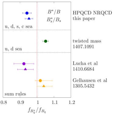
Figure 7: A comparison of recent results for the ratio of vector to pseudoscalar decay constants for $B^{*}/B$ (filled circles) and $B^{*}_{s}/B_{s}$ (filled triangles). The top two results (in blue) are from this paper. The filled green triangle is a lattice QCD result using twisted mass quarks Becirevic et al. (2014) to interpolate beween $c$ and the infinite mass limit. The lowest two sets of results in purple and orange use QCD sum rules Lucha et al. (2014b); Gelhausen et al. (2013). The red dashed line marks the value 1.0.

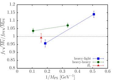
Figure 8: The ratio of $f\sqrt{M}$ for vector and pseudoscalar mesons with at least one heavy quark, plotted against the inverse of the mass for the pseudoscalar meson. Filled blue squares give the results obtained here for the $B^{*}_{s}/B_{s}$ along with the results from Donald et al. (2014b) for $f_{D^{*}_{s}}/f_{D_{s}}$ multiplied by the square root of the ratio of the meson masses from experiment Olive et al. (2014). Filled green circles give the results for heavy-heavy mesons using experimental values for the vector decay constant obtained from the leptonic width Olive et al. (2014) and results from lattice QCD using HISQ quarks for the pseudoscalar Davies et al. (2010a); McNeile et al. (2012a). The filled red triangle gives the result from this paper for the $B^{*}_{c}/B_{c}$ ratio.

Naively we expect heavy mesons with the same valence quark content but with vector or pseudoscalar quantum numbers to be very similar since spin-dependent (hyperfine) intereactions that distinguish between quark and antiquark having spins parallel or anti-parallel are suppressed by the quark mass. Such arguments in respect of the meson masses are straightforward to make even within the quark model. For NRQCD the dominant source of such effects for the vector to pseudoscalar meson mass difference is the term proportional to $c_{4}$ in the NRQCD Hamiltonian, eq. (2) Dowdall et al. (2012b); Dowdall et al. (2014).

For decay constants the arguments are more subtle which is why lattice QCD calculations are important to pin down the results. Viewed from the perspective of a nonrelativistic effective theory, there are three sources for terms that affect the ratio of vector to pseudoscalar decay constants for heavy mesons: one is the hyperfine term in the Hamiltonian as above, the second is the relativistic current correction terms ($J^{(1)}$ in eq. 5) and the third is matching of the current operator to full QCD. The first two give an effect that is proportional to $\Lambda/m_{h}$ whereas the third gives corrections to 1 that are proportional to $\alpha_{s}$. The different dependence of the three effects and the possibilities of cancellation between them have given rise to a variety of predictions for the ratio of decay constants for vector and pseudoscalar heavy-light mesons over the years and controversy has surrounded the question of whether the ratio is larger or smaller than 1 at the $b$ quark mass. Our results here show that the ratio is less than 1 (to $2\sigma$) for $B^{*}/B$ and $B^{*}_{s}/B_{s}$ mesons. In this subsection we set this in the context of earlier results.

A baseline that can be used for heavy-light mesons Neubert (1992) is Heavy Quark Effective Theory (HQET) in which the quark Lagrangian becomes simple, with no spin dependence, in the infinite quark mass limit. The matrix elements of the spatial vector and temporal axial currents between the vacuum and heavy-light mesons become the same in this limit within the effective theory but the renormalisation factors that match the currents to full QCD are not the same. These have been calculated through ${\mathcal{O}}(\alpha_{s}^{2})$ in Broadhurst and Grozin (1995) and through ${\mathcal{O}}(\alpha_{s}^{3})$ in Bekavac et al. (2010) giving, to this leading nonrelativistic order and in terms of the $\overline{MS}$ coupling Bekavac et al. (2010):

$$\left.\frac{f_{B}^{*}}{f_{B}}\right|_{\mathrm{HQET,LO}}=1 - \frac{2\alpha^{(4)}_{s}(m_{b})}{3\pi}$$

$$- (6.370+0.189)\left(\frac{\alpha^{(4)}_{s}(m_{b})}{\pi}\right)^{2}$$

$$- (77.549+6.575)\left(\frac{\alpha^{(4)}_{s}(m_{b})}{\pi}\right)^{3}$$

$$+ \mathcal{O}(\alpha_{s}^{4}).$$

This is evaluated for $u$, $d$, $s$ and $c$ quarks in the sea with the second term in the $\alpha_{s}^{2}$ and $\alpha_{s}^{3}$ coefficients taking account of the non-zero mass for the $c$ quark. Evaluating the expression in eq. (IV) gives 0.896 Bekavac et al. (2010), well below 1.0.

Early calculations added sum-rule estimates of $\Lambda/m_{h}$ hyperfine and current corrections to the one-loop piece of eq. (IV) and obtained a variety of results depending on the relative sign of hyperfine and current correction terms. In Ball (1994) it was found that the hyperfine and current corrections terms have opposite sign (in agreement with a subsequent lattice NRQCD study Collins et al. (1997)) and this gave a vector to pseudoscalar decay constant ratio for $b$-light mesons of 1.00(4). The central value in this result would be reduced below 1.0 using the three-loop expression above.

The calculation we give here improves on this approach since it is a fully integrated calculation in lattice QCD, including dynamics for the $b$ quark from the outset. We use an improved NRQCD action for the $b$ quark accurate (for heavy-light calculations) through $\mathcal{O}(\alpha_{s}\Lambda/m_{h})$ which has been tested on the heavy-light meson spectrum Dowdall et al. (2012b) and from which we can calculate the matrix elements of current operators nonperturbatively. The nonrelativistic current, combining the leading term and first, $\Lambda/m_{b}$, relativistic correction is matched to full QCD and the $\mathcal{O}(\alpha_{s})$ matching correction is found to be very small.

Our results, as described in Subsection III.1, show that $f_{B^{*}_{s}}/f_{B_{s}}$ and $f_{B^{*}}/f_{B}$ are about 5.0(2.5)% below 1, and the ratio for the $B^{*}/B$ is 1.3(1.4)% below that of the $B^{*}_{s}/B_{s}$. Our values are compared to results from two recent QCD sum-rule analyses Lucha et al. (2014b); Gelhausen et al. (2013) in Figure 7. Although there is some tension, those results are consistent with each other and with our numbers here. All the results show the same tendency for the ratio for $B^{*}/B$ to be slightly smaller than for $B^{*}_{s}/B_{s}$, although the difference is not significant in any of the cases.

We also compare to a recent lattice QCD result Becirevic et al. (2014) which used the twisted-mass formalism for both heavy and light quarks on gluon field configurations that included the effect of $u/d$ quarks (only) in the sea. The twisted-mass value is obtained from results calculated for heavy quark masses around the $c$ quark mass and above. An interpolation between those results and the infinite mass limit is performed to reach the $b$, using the first two-loops of the three-loop formula of eq. (IV) to rescale results so that 1.0 (up to higher-order corrections) is obtained in the infinite mass limit. The value quoted for $f_{B^{*}}/f_{B}$ is 1.051(17) and this disagrees with our value by more than 3 (combined) standard deviations. It is not clear that results using only $u/d$ quarks in the sea will necessarily agree with those, like ours, that include a full complement of sea quarks. This may be a case where the ‘quenching’ of the $s$ quark produces a visible effect. A more likely source of difference is probably the interpolation in Becirevic et al. (2014) between the charm mass and the infinite mass limits. Such an interpolation requires evaluating the formula of eq. (IV) using $\alpha_{s}$ at a scale much lower than $m_{b}$ where the relatively large coefficients make that problematic.

It is also interesting to compare results for the ratio of vector to pseudoscalar decay constants between heavy-heavy mesons and heavy-light mesons. The decay constant of vector heavyonium mesons can be determined from their experimental decay rate to leptons:

$$\Gamma(v_{h}\rightarrow e^{+}e^{-})=\frac{4\pi}{3}\alpha_{\mathrm{QED}}^{2}e_{h}^{2}\frac{f_{v}^{2}}{m_{v}}.$$ (26)

The decay constants can also be calculated in lattice QCD Becirevic and Sanfilippo (2013); Donald et al. (2012); Colquhoun et al. (2015) and good agreement with experiment is found. Since heavyonium pseudoscalar mesons do not annihilate to a single particle, there is no direct experimental determination of the decay constant. Again, however, the decay constants can be accurately determined in lattice QCD Davies et al. (2010a); McNeile et al. (2012a).

Figure 8 shows the ratio of vector to pseudoscalar decay constants (multiplied by the square root of the ratio of the masses) for $(J/\psi)/\eta_{c}$, $\Upsilon/\eta_{b}$, $B^{*}_{s}/B_{s}$ and $D_{s}^{*}/D_{s}$ plotted against the inverse of the corresponding pseudoscalar meson mass. For the $J/\psi$ and $\Upsilon$ decay constants we use the values determined from the experimental annihilation rates Olive et al. (2014) and eq. (26). These are 0.407(5) GeV and 0.689(5) GeV respectively. From full lattice QCD the $\eta_{c}$ decay constant is 0.3947(24) GeV Davies et al. (2010a) and the $\eta_{b}$ decay constant is 0.667(6) GeV McNeile et al. (2012a). The $D_{s}^{*}/D_{s}$ decay constant ratio is taken from Donald et al. (2014b). We see that the behaviour for heavyonium and heavy-light mesons is similar but the slope is larger for heavy-light mesons.

For heavyonium mesons, similar considerations apply to the decay constant ratio as discussed above for heavy-light mesons. A baseline might be considered a simple spin-independent potential model in which the decay constant can be related to the ‘wavefunction-at-the-origin’. However there are significant QCD radiative corrections to match $\psi(0)$ to the decay constant in both the vector (see, for example Barbieri et al. (1976)) and pseudoscalar Braaten and Fleming (1995) cases, and these need to be included. Going beyond this requires the inclusion of spin-dependent terms in the Hamiltonian and relativistic corrections to the leading-order current. These are taken care of in a lattice QCD calculation, either explicitly when using a nonrelativistic formalism such as NRQCD Colquhoun et al. (2015) or implicitly included when using a relativistic formalism such as HISQ McNeile et al. (2012a).

Here we have calculated the decay constant of both the $B_{c}$ and the $B^{*}_{c}$, using NRQCD $b$ quarks and HISQ $c$ quarks and working through first-order in the QCD matching and relativistic spin-dependent corrections to the NRQCD Hamiltonian and the currents. Our result for the $B_{c}$ decay constant agrees well with that obtained previously using the relativistic HISQ formalism for both $b$ and $c$ quarks McNeile et al. (2012a), adding confidence to our analysis of systematic errors in both the nonrelativistic and relativistic approach. Here we also calculate the ratio of decay constants for the $B_{c}^{*}$ and $B_{c}$, for the first time from lattice QCD.

$B_{c}$ and $B^{*}_{c}$ decay constants have also been calculated within a potential-model approach, including QCD radiative corrections. See Kiselev (2004) for a discussion. Results are in reasonable agreement with ours, but with a larger uncertainty because the approach has less control of systematic errors.

We find a value for $f_{B^{*}_{c}}/f_{B_{c}}$ which is larger than that of $f_{B^{*}_{s}}/f_{B_{s}}$, indicating that the internal structure of the $B_{c}$ is somewhat different from that of a typical heavy-light meson. Figure 8 shows this clearly. When the decay constant ratio is plotted for the $B^{*}_{c}/B_{c}$ it lies very neatly between the heavy-heavy line and the heavy-light line.

V Conclusions

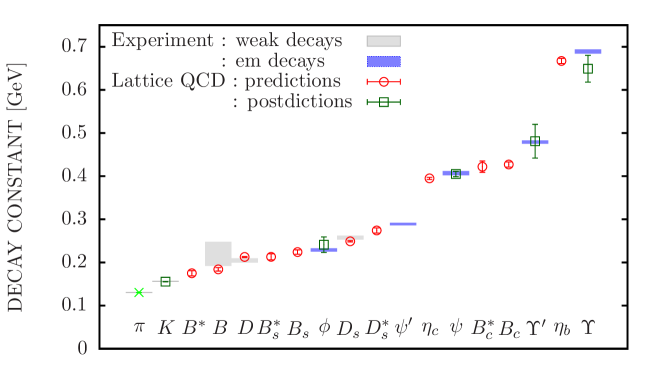
Figure 9: A summary of values for decay constants of mesons that are narrow and so well-characterised in experiment. Experimental values are given as blue or grey bands and are taken from average weak or electromagnetic annihilation rates Olive et al. (2014) using, for weak decays, average values of the appropriate CKM matrix element. For full lattice QCD results, green open squares (postdictions) or red open circles (predictions), we take world’s best values. The lattice result for $f_{\pi^{+}}$ is marked with a cross to indicate that it is used to set the scale in some analyses (although not here). The result for the $K^{+}$ is from Dowdall et al. (2013b), the $B^{+}$ and $B_{s}$ from Dowdall et al. (2013a), the $D^{+}$ and $D_{s}$ from Bazavov et al. (2014), the $\phi$ from Donald et al. (2014a), the $D^{*}_{s}$ from Donald et al. (2014b), the $\eta_{c}$ from Davies et al. (2010a), the $J/\psi$ from Donald et al. (2012), the $B_{c}$ and $\eta_{b}$ from McNeile et al. (2012a), the $\Upsilon$ and $\Upsilon^{\prime}$ from Colquhoun et al. (2015) and the $B^{*}$, $B^{*}_{s}$ and $B^{*}_{c}$ from this paper.

Decay constants, which parameterise the amplitude for a meson to annihilate to a single particle, are as much a part of a meson’s ‘fingerprint’ as its mass. They are often harder to determine, however, and some cannot be accessed directly through an experimental decay rate. The overall picture of meson decay constants gives information about how the internal structure of mesons changes for different quark configurations as a result of QCD interactions. To obtain this picture in sufficient detail, for example even to put the decay constants into an order, requires calculations in full lattice QCD, since only then can we reliably quantify the systematic errors.

Here we have expanded range of decay constant calculations from full lattice QCD to include vector heavy-light mesons. Our results for the ratio of vector to pseudoscalar decay constants are:

$$\frac{f_{B^{*}}}{f_{B}} = 0.941(26)$$ (27)

$$\frac{f_{B^{*}_{s}}}{f_{B_{s}}} = 0.953(23)$$

$$\frac{f_{B^{*}_{c}}}{f_{B_{c}}} = 0.988(27).$$

Thus

• The vector decay constant is smaller than the pseudoscalar decay constant for $b$-light mesons, at the $2\sigma$ level for $B^{*}/B$ and $B^{*}_{s}/B_{s}$. This is in contrast to results for $c$-light mesons where the vector has a larger decay constant than the pseudoscalar.

• The ratio of vector to pseudoscalar decay constants shows an ordering so that $f_{B^{*}_{c}}/f_{B_{c}}>f_{B^{*}_{s}}/f_{B_{s}}>f_{B^{*}}/f_{B}$. When correlations between the uncertainties are taken into account using ratios, the first of these relationships has $3\sigma$ significance, the second $1\sigma$ (see eqs. (22) and (16)).

Using our earlier world’s best results for $f_{B}$ (0.186(4) GeV, isospin-averaged), $f_{B_{s}}$ (0.224(5) GeV) Dowdall et al. (2013a) and $f_{B_{c}}$ (0.427(6) GeV) McNeile et al. (2012a) we derive values for the vector decay constants:

$$f_{B^{*}} = 0.175(6)\,\mathrm{GeV}$$ (28)

$$f_{B^{*}_{s}} = 0.213(7)\,\mathrm{GeV}$$

$$f_{B^{*}_{c}} = 0.422(13)\,\mathrm{GeV}.$$

Finally, in Figure 9 we give a ‘spectrum’ plot for the decay constants of 15 gold-plated mesons from lattice QCD, including the new results from this paper. It illustrates the coverage and predictive power of lattice QCD calculations. The decay constants are ordered by value, something that is only possible with sufficiently accurate results. The range of values is much smaller than that for meson masses and the ordering of values is not as obvious because the quark masses do not have the same impact on the decay constants as they do on the meson masses. The plot therefore shows up some interesting features in the ordering, for example that the $K$ and $B^{*}$ mesons have such similar values and that the $\phi$ meson appears so far up the list. We see that the decay constants for vector-pseudoscalar pairs are close together everywhere, closer than for the pairings in which an $s$ quark is substituted for a light quark in a meson, for example.

Future work will improve the accuracy of lattice QCD results for the vector-onium states such as the $\phi$ (not strictly gold-plated) Chakraborty et al. (2014) and the $\psi^{\prime}$ Galloway et al. (2014), both of which can be determined accurately from experiment. The issues there are mainly from lattice QCD statistical errors. For $b$-light meson decay constants the dominant source of uncertainty, as we have seen, is from systematic errors in NRQCD such as current renormalisation factors. Work is underway to reduce these further using techniques based on current-current correlator methods Colquhoun et al. (2015); Koponen et al. (2010).

References

- Davies (2011) C. Davies, PoS LATTICE2011, 019 (2011), eprint 1203.3862.
- Olive et al. (2014) K. Olive et al. (Particle Data Group), Chin. Phys. C38, 090001 (2014).
- Becirevic et al. (2014) D. Becirevic, A. L. Yaouanc, A. Oyanguren, P. Roudeau, and F. Sanfilippo (2014), eprint 1407.1019.
- Lucha et al. (2014a) W. Lucha, D. Melikhov, and S. Simula (2014a), eprint 1411.3890.
- Dowdall et al. (2013a) R. Dowdall, C. Davies, R. Horgan, C. Monahan, and J. Shigemitsu (HPQCD Collaboration), Phys.Rev.Lett. 110, 222003 (2013a), eprint 1302.2644.
- Dowdall et al. (2012a) R. Dowdall, B. Colquhoun, J. Daldrop, C. Davies, et al. (HPQCD Collaboration), Phys.Rev. D85, 054509 (2012a), eprint 1110.6887.
- Follana et al. (2007) E. Follana, Q. Mason, C. Davies, K. Hornbostel, et al. (HPQCD Collaboration), Phys.Rev. D75, 054502 (2007), eprint hep-lat/0610092.
- McNeile et al. (2012a) C. McNeile, C. Davies, E. Follana, K. Hornbostel, and G. Lepage (HPQCD Collaboration), Phys.Rev. D86, 074503 (2012a), eprint 1207.0994.
- Donald et al. (2014a) G. Donald, C. Davies, J. Koponen, and G. Lepage (HPQCD Collaboration), Phys.Rev. D90, 074506 (2014a), eprint 1311.6669.
- Dowdall et al. (2012b) R. Dowdall, C. Davies, T. Hammant, and R. Horgan (HPQCD Collaboration), Phys.Rev. D86, 094510 (2012b), eprint 1207.5149.
- Davies (1993) C. Davies (UKQCD Collaboration), Proceedings of Lattice93 p. 437 (1993), eprint hep-lat/9312020.
- Bazavov et al. (2010) A. Bazavov et al. (MILC collaboration), Phys.Rev. D82, 074501 (2010), eprint 1004.0342.
- Bazavov et al. (2013) A. Bazavov et al. (MILC Collaboration), Phys.Rev. D87, 054505 (2013), eprint 1212.4768.
- Follana et al. (2008) E. Follana, C. T. H. Davies, G. P. Lepage, and J. Shigemitsu (HPQCD Collaboration), Phys. Rev. Lett. 100, 062002 (2008), eprint 0706.1726.
- Hart et al. (2009) A. Hart, G. M. von Hippel, and R. R. Horgan (HPQCD Collaboration), Phys. Rev. D79, 074008 (2009), eprint 0812.0503.
- Bazavov et al. (2014) A. Bazavov et al. (Fermilab Lattice, MILC Collaborations), Phys.Rev. D90, 074509 (2014), eprint 1407.3772.
- McNeile et al. (2010) C. McNeile, C. T. H. Davies, E. Follana, K. Hornbostel, and G. P. Lepage (HPQCD Collaboration), Phys. Rev. D82, 034512 (2010), eprint 1004.4285.
- Chakraborty et al. (2015) B. Chakraborty, C. Davies, B. Galloway, P. Knecht, J. Koponen, et al., Phys.Rev. D91, 054508 (2015), eprint 1408.4169.
- Lepage et al. (1992) G. Lepage, L. Magnea, C. Nakhleh, U. Magnea, and K. Hornbostel, Phys.Rev. D46, 4052 (1992), eprint hep-lat/9205007.
- Hammant et al. (2011) T. C. Hammant, A. G. Hart, G. M. von Hippel, R. R. Horgan, and C. J. Monahan, Phys. Rev. Lett. 107, 112002 (2011), eprint 1105.5309.
- Daldrop et al. (2012) J. Daldrop, C. Davies, and R. Dowdall (HPQCD Collaboration), Phys.Rev.Lett. 108, 102003 (2012), eprint 1112.2590.
- Dowdall et al. (2014) R. Dowdall, C. Davies, T. Hammant, and R. Horgan (HPQCD collaboration), Phys.Rev. D89, 031502 (2014), eprint 1309.5797.
- Gray et al. (2005) A. Gray, I. Allison, C. Davies, E. Dalgic, G. Lepage, et al. (HPQCD Collaboration), Phys.Rev. D72, 094507 (2005), eprint hep-lat/0507013.
- Gregory et al. (2011) E. B. Gregory, C. T. Davies, I. D. Kendall, J. Koponen, K. Wong, et al. (HPQCD Collaboration), Phys.Rev. D83, 014506 (2011), eprint 1010.3848.
- Lepage and Mackenzie (1993) G. Lepage and P. B. Mackenzie, Phys.Rev. D48, 2250 (1993), phys. Lett. B., eprint hep-lat/9209022.
- Davies et al. (2010a) C. Davies, C. McNeile, E. Follana, G. Lepage, et al. (HPQCD Collaboration), Phys.Rev. D82, 114504 (2010a), eprint 1008.4018.
- Davies et al. (2010b) C. Davies, E. Follana, I. Kendall, G. P. Lepage, and C. McNeile (HPQCD Collaboration), Phys.Rev. D81, 034506 (2010b), eprint 0910.1229.
- Dowdall et al. (2013b) R. Dowdall, C. Davies, G. Lepage, and C. McNeile (HPQCD Collaboration), Phys.Rev. D88, 074504 (2013b), eprint 1303.1670.
- Wingate et al. (2003) M. Wingate, J. Shigemitsu, C. T. Davies, G. P. Lepage, and H. D. Trottier, Phys.Rev. D67, 054505 (2003), eprint hep-lat/0211014.
- Lepage et al. (2002) G. Lepage, B. Clark, C. Davies, K. Hornbostel, P. Mackenzie, et al., Nucl.Phys.Proc.Suppl. 106, 12 (2002), eprint hep-lat/0110175.
- Monahan et al. (2013) C. Monahan, J. Shigemitsu, and R. Horgan, Phys.Rev. D87, 034017 (2013), eprint 1211.6966.
- Harada et al. (2002) J. Harada, S. Hashimoto, K.-I. Ishikawa, A. S. Kronfeld, T. Onogi, et al., Phys.Rev. D65, 094513 (2002), eprint hep-lat/0112044.
- Chakraborty et al. (2014) B. Chakraborty, C. Davies, G. Donald, R. Dowdall, J. Koponen, et al. (HPQCD collaboration), PoS LATTICE2013, 309 (2014), eprint 1401.0669.
- Collins et al. (1997) S. Collins, U. M. Heller, J. Sloan, J. Shigemitsu, A. Ali Khan, and C. Davies, Phys.Rev. D55, 1630 (1997), eprint hep-lat/9607004.
- Collins et al. (1999) S. Collins, C. Davies, U. M. Heller, A. Ali Khan, J. Shigemitsu, et al., Phys.Rev. D60, 074504 (1999), eprint hep-lat/9901001.
- Ball (1994) P. Ball, Nucl.Phys. B421, 593 (1994), eprint hep-ph/9312325.
- Neubert (1992) M. Neubert, Phys.Rev. D46, 1076 (1992).
- Gregory et al. (2010) E. Gregory, C. Davies, E. Follana, E. Gamiz, I. Kendall, et al. (HPQCD Collaboration), Phys.Rev.Lett. 104, 022001 (2010), eprint 0909.4462.
- McNeile et al. (2012b) C. McNeile, C. Davies, E. Follana, K. Hornbostel, and G. Lepage (HPQCD Collaboration), Phys.Rev. D85, 031503 (2012b), eprint 1110.4510.
- Aaij et al. (2013) R. Aaij et al. (LHCb), Phys.Rev. D87, 112012 (2013), eprint 1304.4530.
- Donald et al. (2014b) G. Donald, C. Davies, J. Koponen, and G. Lepage (HPQCD Collaboration), Phys.Rev.Lett. 112, 212002 (2014b), eprint 1312.5264.
- Donald et al. (2012) G. Donald, C. Davies, R. Dowdall, E. Follana, K. Hornbostel, et al. (HPQCD Collaboration), Phys.Rev. D86, 094501 (2012), eprint 1208.2855.
- Lucha et al. (2014b) W. Lucha, D. Melikhov, and S. Simula, EPJ Web Conf. 80, 00046 (2014b), eprint 1410.6684.
- Gelhausen et al. (2013) P. Gelhausen, A. Khodjamirian, A. A. Pivovarov, and D. Rosenthal, Phys.Rev. D88, 014015 (2013), eprint 1305.5432.
- Broadhurst and Grozin (1995) D. J. Broadhurst and A. Grozin, Phys.Rev. D52, 4082 (1995), eprint hep-ph/9410240.
- Bekavac et al. (2010) S. Bekavac, A. Grozin, P. Marquard, J. Piclum, D. Seidel, et al., Nucl.Phys. B833, 46 (2010), eprint 0911.3356.
- Becirevic and Sanfilippo (2013) D. Becirevic and F. Sanfilippo, JHEP 1301, 028 (2013), eprint 1206.1445.
- Colquhoun et al. (2015) B. Colquhoun, R. Dowdall, C. Davies, K. Hornbostel, and G. Lepage, Phys.Rev. D91, 074514 (2015), eprint 1408.5768.
- Barbieri et al. (1976) R. Barbieri, R. Kogerler, Z. Kunszt, and R. Gatto, Nucl.Phys. B105, 125 (1976).
- Braaten and Fleming (1995) E. Braaten and S. Fleming, Phys.Rev. D52, 181 (1995), eprint hep-ph/9501296.
- Kiselev (2004) V. Kiselev, Central Eur.J.Phys. 2, 523 (2004), eprint hep-ph/0304017.
- Galloway et al. (2014) B. Galloway, P. Knecht, J. Koponen, C. Davies, and G. P. Lepage (HPQCD collaboration), PoS LATTICE2014, 092 (2014), eprint 1411.1318.
- Koponen et al. (2010) J. Koponen, C. Davies, K. Hornbostel, et al. (HPQCD), PoS LATTICE2010, 231 (2010), eprint 1011.1208.