Abstract.The article deals with the mathematical model for media with hierarchical structure. Using the hamiltonian formalism, the dynamical system describing the state of hierarchically connected structural elements was derived. According to the analysis of the Poincaré sections, we found the localized quasi-periodic and chaotic trajectories in the three-level hierarchical model. Moreover, studies of correlation functions shown that the power spectrum for three-level model possesses local maxima characterizing temporal scales with strong correlation. Using the Fourier analysis of the solution’s components, we have studied the distribution of energy injected in the system over hierarchical levels. Dynamical phenomena in the multi-level system were studied as well.

1 Introduction

One productive way to study dynamic processes in the lithosphere is an approach in which the lithosphere is considered as a hierarchical system of volumes (blocks) [1, 2, 3, 4, 5], where the block sizes are scaled in the interval from kilometers (tectonic plates) to millimeters (grains of rocks). The main features of dynamic behavior of such systems are high degree of nonlinearity, complicated interaction between structural elements, the redistribution of energy between hierarchical levels. These processes are manifested in the generation of high-frequency oscillations during the application of low-frequency disturbances in near - wellbore area [6], in the change of spectra of aftershocks sequences [7], in the existence of a wide range of nonlinear waves after explosions in rock massifs [8] and so on. The exchange of energy between hierarchical levels is the significant factor in the loss of stability of block systems during seismic energy release [9, 10]. In order to study these dynamical phenomena, we propose a model for media consisting of the hierarchically connected elements (blocks). Most studies of the dynamics of hierarchical systems of oscillators have been focused on the synchronization processes [11, 12, 13, 14, 15, 16, 17, 18, 19, 20, 21, 22], instead we are interested in exploring exchange of energy between hierarchical levels, in particular, energy transfer from the upper level to the lower one.

The rest of this report is organized as follows. In Sec.2 we introduce the models describing the hierarchically connected oscillators. Using the Poincaré section technique, correlation and spectral analysis, in Sec.3 we investigate the simplified model for three-level system of oscillators. Sec. 4 is devoted to dynamical phenomena being observed in the multi-level hierarchical system when model parameters are varied. Concluding remarks are incorporated in final Sec.5.

2 Models for hierarchical media

We model the hierarchical block medium by the embedded system of anharmonic oscillators (Fig. 1a). The part of hierarchical system as a tree is shown in Fig.1b.

Assume that the model incorporates $N$ levels and each oscillator from $n$th $(1<n<N)$ level connects with $s$ oscillators from the $(n+1)$th level, except the lowest level oscillators. The Hamiltonian of this system has the following form

$$H=\sum\limits_{n=1}^{N}{\sum\limits_{k=1}^{k_{n}}{\left({\frac{p_{nk}^{2}}{2m_{nk}}+\frac{C_{nk}}{\alpha}\left|{x_{nk}-x_{(n-1)\ell_{k}}}\right|^{\alpha}}\right)}},$$ (1)

where index $(nk)$ denotes the oscillator’s position, namely, the $n$th level and the $k$th place; $\ell_{k}$ is the place of oscillator from the $(n-1)$th level connected with the $(nk)$th oscillator; $m_{nk}$ and $p_{nk}$ are the mass and, respectively, the momentum of the $(nk)$th oscillator; $x_{nk}$ is the oscillator’s coordinate; $C_{nk}$ is the stiffness of link, $\alpha$ is a constant.

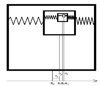
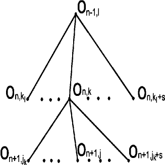
a                                                                       b

Figure 1: The model of hierarchical medium (a) and corresponding tree (b).

Inserting $H$ into the equations

$$\dot{x}_{nk}=\frac{{\partial H}}{{\partial p_{nk}}},\quad\dot{p}_{nk}=-\frac{{\partial H}}{{\partial x_{nk}}},$$

one can obtain the following system of differential equations

$$\begin{split}\dot{x}_{nk}&=p_{nk}/m_{nk},\\ \dot{p}_{nk}&=-C_{nk}\left|{x_{nk}-x_{(n-1)\ell_{k}}}\right|^{\alpha-1}\mbox{sgn}(x_{nk}-x_{(n-1)\ell_{k}})\\ &+\sum_{j}^{j+s}C_{(n+1)j}\left|{x_{(n+1)j}-x_{nk}}\right|^{\alpha-1}\mbox{sgn}(x_{(n+1)j}-x_{(n+1)k}),\end{split}$$ (2)

where $\mbox{sgn}(x)=1$ if $x\geq 0$, otherwise $\mbox{sgn}(x)=-1$. Considering the oscillators, which are identical on each level and move synchronously, system (2) can be written as follows

$$\begin{split}\ddot{x}_{n}=-\omega_{n}^{2}\left|{x_{n}-x_{n-1}}\right|^{\alpha-1}\mbox{sgn}(x_{n}-x_{n-1})+\omega_{n+1}^{2}s\frac{m_{n+1}}{m_{n}}\left|{x_{n+1}-x_{n}}\right|^{\alpha-1}\mbox{sgn}(x_{n+1}-x_{n}),\end{split}$$ (3)

where $\omega_{n}^{2}=\frac{C_{n}}{m_{n}}$.

For convenience, let us introduce the new variables $q_{n}=x_{n}-x_{n-1}$ having the meaning of displacements from the steady state, $x_{0}=\mbox{const}$. Then $x_{n}=\sum_{s=1}^{N}q_{s}$. Finally, system (3) reads

$$\begin{split}\sum_{s=1}^{N}\ddot{q}_{s}=&-\omega_{i}^{2}\left|q_{i}\right|^{\beta}\mbox{sgn}(q_{i})+\omega_{i+1}^{2}s\frac{m_{i+1}}{m_{i}}\left|{q_{i+1}}\right|^{\beta}\mbox{sgn}(q_{i+1}).\end{split}$$ (4)

Using the designations $F_{i}=\omega_{i}^{2}\left|q_{i}\right|^{\beta}\mbox{sgn}(q_{i})$, $\varphi_{i}=sm_{i+1}/m_{i}$, we present system (4) in the form

$$\begin{split}\ddot{q}_{1}=-F_{1}+\phi_{1}F_{2},\\ \ddot{q}_{n}=F_{n-1}-F_{n}(1+\varphi_{n-1})+\varphi_{n}F_{n+1},\\ \ddot{q}_{N}=F_{N-1}-F_{N}(1+\varphi_{N-1}).\end{split}$$ (5)

For simplicity, we assume that the quantities $\omega_{i}$ and $m_{i}$ are the geometric sequences. So, $\omega_{i}=\omega_{0}r^{i-1}$, $r>1$, and $m_{i}=m_{0}h^{i-1}$, $h<1$. From this it follows that $\varphi_{i}=sh=\varphi=\mbox{const}$.

3 Studies of the model with three hierarchical levels

To begin with, let us consider the model with three hierarchical levels, i.e. putting $N=3$. In this case system (5) has the following form

$$\begin{split}\ddot{q}_{1}=-F_{1}+\varphi F_{2},\\ \ddot{q}_{2}=F_{1}-F_{2}(1+\varphi)+\varphi F_{3},\\ \ddot{q}_{3}=F_{2}-F_{3}(1+\varphi).\end{split}$$ (6)

Till now we did not achieve success in finding any exact solutions to system (6). Therefore, in order to get the information on the solutions structure, we are going to use the numerical and qualitative analysis methods.

Due to the Hamiltonian nature of system (6), the trajectories of the dynamical system lay on constant energy hyper-surfaces. The allocation of these hyper-surfaces in the phase space can be effectively studied by means of the Poincaré section technique [23, 27].

3.1 The sequence of frequencies $\omega_{i}=r^{i-1}$, $r=1.1$

Let us fix the parameters $\omega_{0}=1$, $r=1.1$, $\varphi=0.6$ and choose the initial conditions for numerical integration in the form of $q_{1}(0)=0$, $q_{1}^{\prime}(0)=0.2$, $q_{j}(0)=q_{j}^{\prime}(0)=0$, $j=2,3$. At first, consider the linear case when $\beta=1$. Let the plane $q_{1}^{\prime}=0$ be the Poincaré section plane. Integrating of system (3) by means of the Dormand-Prince method [26], we are interested in the points in which trajectories intersect the cross-plane in one direction only. Mapping this section onto the plane $(q_{2}^{\prime};q_{1})$, we obtain the diagrams presented in the figure 2a. The figure 2b corresponds to the Poincaré section of the trajectory beginning at the same starting point as in previous case but the parameter $\beta=1.05$.

In the same manner, putting $\beta=1.1$, $\beta=1.15$, $\beta=1.25$, and $\beta=1.5$ (the nonlinear cases), we obtain the typical Poincaré diagrams depicted in the Figs.2-3.

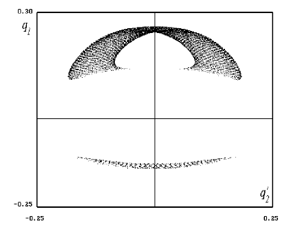
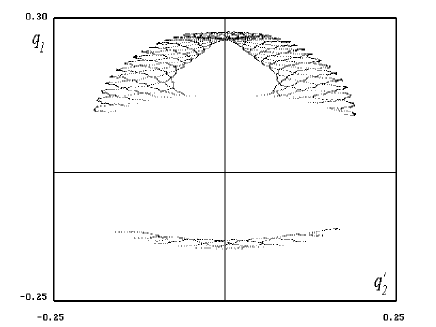
a                                                                       b

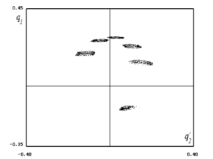
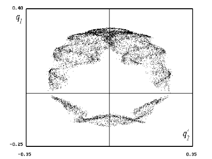
c                                                                       d

Figure 2: Poincaré sections at different $\beta=1$ (a), $\beta=1.05$ (b), $\beta=1.10$ (c),$\beta=1.15$ (d). Initial conditions $q_{1}^{\prime}=0.2$ and the other coordinates are equal to zero.

From the analysis of these figures it follows that the incorporation of nonlinearity in the model causes the appearance of the striped torus surfaces (Figs.2b), tori with dense winding (Figs.2c), trajectories similar to periodic ones (Figs.3c), which are not observed in the linear case.

According to Fig.3d, the increasing of nonlinearity associated with the parameter $\beta$ leads to the formation of Poincaré sections uniformly filled with points.

Comparing the initial conditions for construction of the Poincaré diagrams of Fig.3, c and d, we see that small deviation of the first coordinate changes the observed regimes essentially. This is one of the main feature of the nonlinear models [28].

It worth noting that the sizes of regimes differ from each other weakly. But there are values of the parameter $\beta$ when the region of the Poincaré section (Fig.3a,b,d) is filled with points nonuniformly. This tells us about existence of prevailing amplitudes in the quasi-periodic regime.

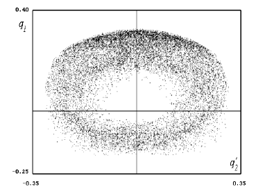
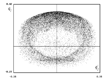
a                                                                       b

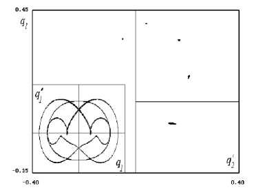
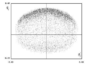
c                                                                       d

Figure 3: Poincaré sections at $\beta=1.20$ (a), $\beta=1.25$ (b), $\beta=1.5$ (c), (d). Initial conditions for (a), (b), (c) $q_{1}^{\prime}=0.2$ and other coordinates are equal to zero. Initial condition for (d): $q_{1}=0.068$, $q_{1}^{\prime}=0.2$, $q_{2,3}=q_{2,3}^{\prime}=0$. In the corner of the figure (c) the quasi-periodic trajectory’s phase portrait corresponding to the Poincaré section (c) is drown.

Additional information on the properties of regimes we study can be obtain with the help of the correlation analysis. Using the solution of system (3) in the form of the discrete sequences $q_{i}(j)$, $i=1,2,3$, $j=1\cdot\tau,2\cdot\tau\ldots,M\cdot\tau$ ($\tau=0.01$ is the step of the temporal variable discretization), we define the cross-correlation function [24]

$$R_{xy}(k)=\frac{M}{M-k}\frac{\sum_{j=1}^{M-k}q_{x}(j)q_{y}(j-k)}{\sum_{j=1}^{M}q_{x}(j)q_{y}(j)},\quad{x,y}=1,\ldots,3.$$

If $x=y$, then we get the definition of the autocorrelation function $R_{xx}(k)$. Together with the correlation functions we use their Fourier transformations $\mbox{FFT}(R_{xy})=S_{xy}(\omega)$ which, in the case of autocorrelation function, coincide with the power spectrum of a signal [25].

Let us begin from the correlation analysis of regimes derived at small $\beta$. Taking the trajectories whose Poincaré sections are depicted in Figs.2a,c, we obtain the graph of $|S_{11}(\omega)|$ (Fig.4a) and $|S_{13}(\omega)|$ (Fig. 4b). According to Fig. 4a, the spectrum has the essential maximum near $\omega=0.1$ and the other one at about $2\omega$. This tells us that the sequence $q_{1}$ possesses the prevailing temporal scale when correlation is the most strong. Note that this dominant frequency displaces to the left at growing nonlinearity (to compare thick and thin curves). Since $\beta$ is small, oscillators’ behavior does not differ from each other (Fig. 4b).

For $\beta=1.5$ when chaotic regime exists (Fig.3d), the spectrum of the function $R_{11}$ has two multiple prevailing frequencies (Fig.4c) which are accompanied by several peaks. At the same time, we observe more essential defragmentation of spectrum for the function $R_{13}$ (Fig.4d). Especially, it should be paid attention to the appearance of additional high-frequency peaks which can be regarded as supplementary temporal scales in media.

3.2 The sequence of frequencies $\omega_{i}=r^{i-1}$, $r=2.0$

Now we are interested in the studies of oscillations in system (3) when the partial frequencies are following $\omega_{i}=r^{i-1}$, $r=2.0$. We keep the same initial conditions for numerical integration as in the previous subsection 3.1.

From the Poincaré sections (Fig.5a) it follows that the trajectories can form the pipe in the phase space at small values of parameter $\beta$. When $\beta$ increases, we observe the transformation of phase space in such a way that the regimes become more chaotic (Fig. 5b,c). Finally, the growth of $\beta$ leads to essential chaotization of the Poincaré section (Fig.5d).

The growth of $\beta$ is thus accompanied by increasing of irregularity. In this situation we can not reduce system (3) to low dimensional model like one dimensional maps generated by Poincaré sections.

To understand phenomena in the system at increasing $\beta$, we derive the Fourier transformations for components $q_{i}$, namely, $FFT(q_{i})$ at $\beta=1.2$ (Fig.6a-c) and $FFT(q_{i})$ at $\beta=1.5$ (Fig.6d-f). From spectra presented in Fig.6a-c it follows that all components $q_{i}$ are characterized by two essential spectral maxima. This causes the existence of torus (Fig.5a) in system’s phase space.

For $\beta=1.5$, the component $q_{1}$ has two wide spectral maxima (Fig.6d) and one notable maximum in the same place as in the spectrum from Fig.6a.

The spectrum of $q_{2}$ (Fig.6e) involves three prevailing maxima having strongly irregular character. In the spectrum of $q_{3}$ we can distinguish three maxima as well. In contrast to the spectrum from Fig.6c, we see that the height of maxima grows as $\omega$ increases. This can be associated with the excitation of the high-frequency spectral modes.

Therefore, system (3) can be regarded as a model describing the directed transport of energy in hierarchical media.

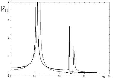
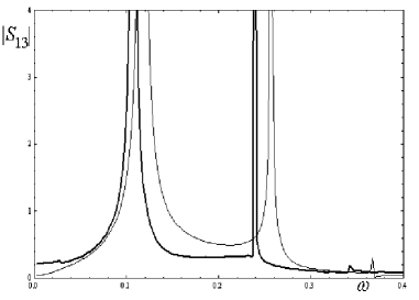
a                                                                       b

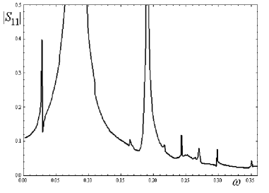
c                                                                       d

Figure 4: The graphs of the functions $|S_{11}(\omega)|$ (left) and $|S_{13}(\omega)|$ (right). The spectra correspond to the regime of Fig. 2c (top panels) and Fig. 3d (bottom panels). The curves depicted by thin lines correspond to linear system (3) with $\beta=1$.

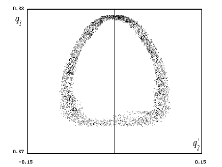
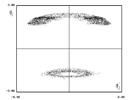
a                                                                       b

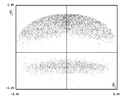
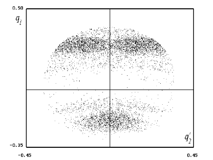
c                                                                       d

Figure 5: Poincaré sections at $\beta=1.2$ (a), $\beta=1.3$ (b), $\beta=1.4$ (c), $\beta=1.5$ (d). The values of parameters $r=2$, $\varphi=0.6$. Initial conditions $q_{1}^{\prime}=0.2$ and the other coordinates are equal to zero.

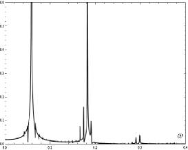
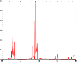
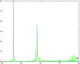
a                                             b                                             c

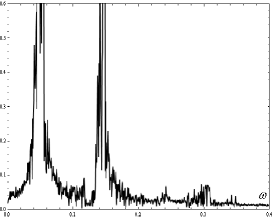
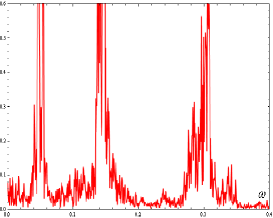
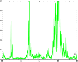
d                                             e                                             f

Figure 6: (color online) Fourier spectra of the $q_{i}$, $i=1,2,3$-component of the trajectories drawn in the Fig. 5 at $\beta=1.2$ and $\beta=1.5$, respectively.

4 Studies of the model with many hierarchical levels

Consider now the model which consists of many hierarchical levels, for instance, $N=20$. The fixed parameters are as follows $\omega_{0}=1$, $r=1.04$, $\beta=1.15$ and initial condition $q_{1}(0)=0$, $q_{1}^{\prime}(0)=0.3$, $q_{j}(0)=q_{j}^{\prime}(0)=0$, $j=2,\ldots,N$. Compare the $q_{1}$ and $q_{N}$ components of solutions to system (3) derived at $\varphi=0.7$ and $\varphi=0.9$. Corresponding results are presented in the left and right panels of figures 7 and 8, respectively.

For $\varphi=0.7$ the amplitude of $q_{1}$ is much less than the amplitude of $q_{N}$. Snapshot from Fig.7a predicts that frequency anatomy of the $q_{1}$ and $q_{N}$ signals is different. Moreover, the $q_{1}$ dynamics looks like a harmonic signal modulated by another signal with higher frequency. This is confirmed by the analysis of Fourier spectra for $q_{1}$ and $q_{N}$ (Fig.8a). The spectrum for $q_{1}$ depicted by thick line in Fig.8a contains one maximum corresponding to existence of mode like a cosine function and a number of much smaller maxima causing a ripple on the $q_{1}$ profile.

As Fig.8a testifies, the spectrum for $q_{N}$ depicted by the red thin curve contains a number of almost equivalent maxima located both in the low and high frequency zones.

Similar analysis can be carried out for the solutions to system (3) at $\varphi=0.9$. Snapshots for the components $q_{1}$ and $q_{N}$ plotted in Fig.7b show that the amplitude of $q_{1}$ is larger than $q_{N}$. According to Fig.8b, the main part of $q_{1}$ Fourier spectrum is localized in low frequency zone. But the spectrum of $q_{N}$ is almost uniformly distributed in the domain under consideration.

From the results presented in this section we can conclude that, at first, a critical value of $\varphi$ can exist corresponding to the formation of comparable oscillations on the first and the last hierarchical levels of media. Secondly, the spectrum of the lowest level we are most interested in is distributed in a wide frequency domain and depending on the $\varphi$ dominant frequencies can be distinguished.

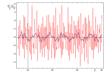
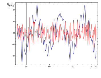
a                                                              b

Figure 7: (color online) Snapshots of the components $q_{1}(t)$ (thick curve) and $q_{N}(t)$ (thin red curve), $t\in(330;500)$ at $\varphi=0.7$ (a) and $\varphi=0.9$ (b).

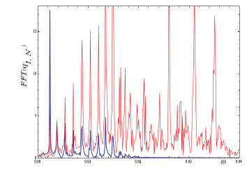
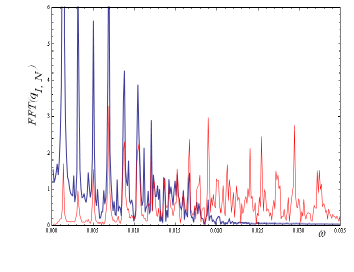
a                                                              b

Figure 8: (color online) Fourier spectra for the components $q_{1}(t)$ (thick curve) and $q_{N}(t)$ (thin red curve) at $\varphi=0.7$ (a) and $\varphi=0.9$ (b).

5 Conclusions

In summary, the strongly nonlinear system of coupled oscillators describing media with hierarchical structure is introduced. The problem we have stated is concerned with the peculiarities of energy transfer along the hierarchical structure of media. To treat this problem, we have studied the phase portraits, correlation functions and Fourier spectra which characterize oscillators placed on different hierarchical levels of media. We thus have seen that hierarchical systems manifest quasiperiodic and chaotic regimes development of which depends on the auxiliary parameter $\varphi$. It is shown that among values of the parameter $\varphi$ corresponding to processes of transferring energy from the top level to the lowest one there is a threshold value. Therefore, within the framework of presented model, one can confirm that the hierarchical structure accompanied by nonlinearity plays an important role in the transformation of energy flows in media. Rearrangement of the hierarchical levels caused by intensive loading is the natural mechanism of accumulation and radiation of energy in structured media under strongly non-equilibrium conditions.

References

- [1] M. Alexeevskaya, A. Gabrielov, I. Gel’fand, A. Gvishiani, E. Rantsman, J. Geoph. 43, 227 (1977)
- [2] M.A. Sadovskii, L.G. Bolhovitinov, V.F. Pisarenko, Izvestiya AN SSSR. Fizika Zemli, 2, 3 (1982) (in Russian)
- [3] A.M. Gabrielov, V.I. Keilis-Borok, T.A. Levshina, V.A. Shaposhnikov, Comp.Seismol, 20, 168 (1986)
- [4] V.I. Keilis-Borok, Rev. Geoph. 28, 19 (1990)
- [5] A.M. Gabrielov, V.I. Keilis-Borok, I. Zaliapin, W.I. Newman, Phys. Rev. E 62, 237 (2000)
- [6] M.V. Kurlenya, J. Mining Sci. 2, 63 (2000) (in Russian)
- [7] M.A. Sadovskii, V.F. Pisarenko, Seismic process in block medium (Nauka, Moscow, 1991) (in Russian)
- [8] M.V. Kurlenya, V.N. Oparin J. Mining Sci. 3, 12 (1999) (in Russian)
- [9] V.I. Starostenko, V.A. Danilenko, D.B. Vengrovitch, K.N. Poplavskii, Tectonophysics 268, 211 (1996)
- [10] M.A. Sadovskii, L.G. Bolhovitinov, V.F. Pisarenko, Deformation of medium and seismic process (Nauka, Moscow, 1987) (in Russian)
- [11] A.T. Winfree, J. Theor. Biol. 16, 15 (1967)
- [12] Y. Kuramoto, Self-entrainment of a population of coupled nonlinear oscillators, in: H. Araki (Ed.), International Symposium on Mathematical Problems in Theoretical Physics, (Springer, New York, 1975) 420
- [13] Y.Kuramoto, Chemical Oscillations, Waves and Turbulence (Springer, New York, 1984)
- [14] J.A. Acebrón, L. L. Bonilla, C. J. Perez Vicente, F. Ritort, R.Spigler, Rev-Modern-Phys, 77, 137 (2005)
- [15] H. Kori, A.S. Mikhailov, Phys. Rev. E 742, 066115 (2006)
- [16] A. Arenas, A. Diaz-Guilera, J. Kurths, Y. Moreno, C. Zhou, Phys. Rep. 469, 93 (2008)
- [17] E. Ott, T. M. Antonsen, Chaos 18, 037113 (2008)
- [18] Z. Zhuo, S.-M. Cai, Z.-Q. Fu, J. Zhang, Phys. Rev E 84, 031923 (2011)
- [19] L. Prignano, A. Diaz-Guilera, Phys. Rev E 85, 036112 (2012)
- [20] P.S. Skardal, J.G. Restrepo, Phys. Rev E 85, 016208 (2012)
- [21] S. Guo, J. Man, J. Differential Equations 254, 3501 (2013)
- [22] P.Villegas, P. Moretti, M.A. Munoz, Sci. Rep. 4, 5990 (2014)
- [23] M. Holodniok, A. Klić, M. Kubićek, M. Marek, Methods of Analysis of Nonlinear Dynamical Models (World Publishing House, Moscow, 1991)
- [24] Percival, Donald B., Andrew T. Walden, Spectral Analysis for Physical Applications: Multitaper and Conventional Univariate Techniques (Cambridge University Press, Cambridge, 1993) 190
- [25] Brown R.G., Hwang P.Y.C. Introduction to Random Signals and Applied Kalman Filtering (John Wiley Sons, 2012)
- [26] E. Hairer, S.P. Nursett, G. Wanner, Solving ordinary differential equations I: Nonstiff problems (Springer-Verlag, Berlin, 2008)
- [27] W.-H. Steeb The nonlinear workbook (World Scientific Publishing, Singapore, 2005)
- [28] E. Ott, Chaos in dynamical systems (Cambridge University Press, Cambridge, 1994)