Asymptotic Efficiency of New Exponentiality Tests Based on a Characterization

Abstract

Two new tests for exponentiality, of integral- and Kolmogorov-type, are proposed. They are based on a recent characterization and formed using appropriate V-statistics. Their asymptotic properties are examined and their local Bahadur efficiencies against some common alternatives are found. A class of locally optimal alternatives for each test is obtained. The powers of these tests, for some small sample sizes, are compared with different exponentiality tests.

keywords: testing of exponentiality, order statistics, Bahadur
efficiency, $U$-statistics

MSC(2010): 60F10, 62G10,  62G20, 62G30.

1 Introduction

Exponential distribution is probably one of the most applicable distribution in reliability theory, survival analysis and many other fields. Therefore, ensuring that the data come from exponential family of distributions is of a great importance. Goodness of fit testing for exponentiality has been popular for decades, and in recent times tests based on characterizations have become one of the primary directions. Many interesting characterizations of exponential distribution can be found in [3], [4], [7] and [8]. Goodness of fit tests based on characterizations of exponential distribution are studied in papers [2], [5], [16], [17], among others. In particular, the Bahadur efficiency of such tests has been considered in, e.g., [20], [26], [29].

Recently Obradović [23] proved three new characterizations of exponential distribution based on order statistics in small samples. In this paper we propose two new goodness of fit tests based on one of those characterizations:

Let $X_{0},X_{1},X_{2},X_{3}$ be independent and identically distributed non-negative random variables (i.i.d.) from the distribution whose density $f(x)$ has the Maclaurin’s expansion for $x>0$. Let $X_{(2;3)}$ and $X_{(3;3)}$ be the median and maximum of $\{X_{1},X_{2},X_{3}\}$. If

$$X_{0}+X_{(2;3)}\overset{d}{=}X_{(3;3)}$$ (1)

then $f(x)=\lambda e^{-\lambda x}$ for some $\lambda>0$.

Let $X_{1},X_{2},\ldots,X_{n}$ be i.i.d. observations having the continuous d.f. $F$. We test the composite hypothesis that $F$ belongs to family of exponential distributions ${\mathcal{E}(\lambda)})$, where $\lambda>0$ is an unknown parameter.

We shall consider integral and Kolmogorov-type test statistics which are invariant with respect to the scale parameter $\lambda$ ( see [15]):

$$I_{n}=\int\limits_{0}^{\infty}\int\limits_{0}^{\infty}(H_{n}(t)-G_{n}(t))dF_{n}(t),$$ (2)

$$K_{n}=\sup\limits_{t\geq 0}\big{|}H_{n}(t)-G_{n}(t)\big{|},$$ (3)

where $G_{n}$ and $H_{n}$ are $V$ empirical d.f.’s

$$G_{n}(t) =\frac{1}{n^{4}}\sum\limits_{i=1}^{n}\sum\limits_{j=1}^{n}\sum\limits_{k=1}^{n}\sum\limits_{l=1}^{n}I\{X_{i}+{\rm med}(X_{j},X_{k},X_{l})<t\},$$

$$H_{n}(t) =\frac{1}{n^{3}}\sum\limits_{j=1}^{n}\sum\limits_{k=1}^{n}\sum\limits_{l=1}^{n}I\{\max(X_{j},X_{k},X_{l})<t\}.$$

In order to determine the quality of our tests and to compare them with some other tests we shall use local Bahadur efficiency. We choose this type of asymptotic efficiency since it is applicable to non-normally distributed test statistics such as Kolmogorov. For asymptotically normally distributed test statistics local Bahadur efficiency and classical Pitman efficiency coincide (see [30]).

The paper is organized as follows. In section 2 we study the integral statistic $I_{n}$. We find its asymptotic distribution, large deviations and calculate its asymptotic efficiency against some common alternatives. We also present a class of locally optimal alternatives. In section 3 we do the analogous study for Kolmogorov-type statistics. In section 4 and 5 we do the comparison of our tests with some existing tests for exponentiality and give the real data example.

2 Integral-type Statistic $I_{n}$

The statistic $I_{n}$ is asymptotically equivalent to $U$-statistic with symmetric kernel ([15])

$$\Psi(X_{1},X_{2},X_{3},X_{4},X_{5})=\frac{1}{5!}\sum\limits_{\pi(1:5)}\big{(}I\{\max(X_{\pi_{2}},X_{\pi_{3}},X_{\pi_{4}})<X_{\pi_{5}}\}$$

$$- I\{X_{\pi_{1}}+{\rm med}(X_{\pi_{2}},X_{\pi_{3}},X_{\pi_{4}})<X_{\pi_{5}}\}\big{)},$$

where $\pi(1:m)$ is the set of all permutations $\{\pi_{1},\pi_{2},...,\pi_{m}\}$ of set $\{1,2,...,m\}$.

Its projection on $X_{1}$ under null hypothesis is

$$\psi(s) = E(\Psi(X_{1},X_{2},X_{3},X_{4},X_{5})|X_{1}=s)$$

$$= \frac{1}{5}\Big{(}P\{\max(X_{2},X_{3},X_{4})<X_{5}\}-P\{s+{\rm med}(X_{2},X_{3},X_{4})<X_{5}\}\Big{)}$$

$$+ \frac{3}{5}\Big{(}P\{\max(s,X_{3},X_{4})<X_{5}\}-P\{X_{2}+{\rm med}(s,X_{3},X_{4})<X_{5}\}\Big{)}$$

$$+ \frac{1}{5}\Big{(}P\{\max(X_{3},X_{4},X_{5})<s\}-P\{X_{2}+{\rm med}(X_{3},X_{4},X_{5})<s\}\Big{)}.$$

After some calculations we get

$$\psi(s)=-\frac{1}{20}+\frac{2}{5}e^{-3s}-\frac{9}{10}e^{-2s}+\frac{1}{2}e^{-s}.$$ (4)

The expected value of this projection is equal to zero, while its variance is

$$\sigma^{2}_{I}=E(\psi^{2}(X_{1}))=\frac{29}{42000}.$$

Hence this kernel is non-degenerate. Applying Hoeffding’s theorem ([12]) we get that the asymptotic distribution of $\sqrt{n}I_{n}$ is normal $\mathcal{N}(0,\frac{29}{1680})$.

2.1 Local Bahadur efficiency

One way of measuring the quality of the tests is calculating their Bahadur asymptotic efficiency. This quantity can be expressed as the ratio of Bahadur exact slope, function describing the rate of exponential decrease for the attained level under the alternative, and double Kullback-Leibler distance between null and alternative distribution. More about theory on this topic can be found in ([6], [19]).

According to Bahadur theory the exact slopes are defined in the following way. Suppose that the sequence $\{T_{n}\}$ of test statistics under alternative converges in probability to some finite function $b(\theta)$. Suppose also that the following large deviations limit exists

$$\lim_{n\to\infty}n^{-1}\ln P_{H_{0}}\left(T_{n}\geq t\right)=-f(t)$$ (5)

for any $t$ in an open interval $I,$ on which $f$ is continuous and $\{b(\theta),\>\theta>0\}\subset I$. Then the Bahadur exact slope is

$$c_{T}(\theta)=2f(b(\theta)).$$ (6)

The exact slopes always satisfy the inequality

$$c_{T}(\theta)\leq 2K(\theta),\,\theta>0,$$ (7)

where $K(\theta)$ is the Kullback-Leibler ”distance” between the alternative $H_{1}$ and the null hypothesis $H_{0}.$

Given (7), the local Bahadur efficiency of the sequence of statistics ${T_{n}}$ is defined as

$$e^{B}(T)=\lim_{\theta\to 0}\frac{c_{T}(\theta)}{2K(\theta)}.$$ (8)

Let $G(\cdot,\theta)$, $\theta\geq 0$, be a family of d.f. with densities $g(\cdot,\theta)$, such that $G(\cdot,0)\in\mathcal{E}(\lambda)$ and the regularity conditions from ([19], Chapter 6), including differentiation along $\theta$ in all appearing integrals, hold. Denote $h(x)=g^{\prime}_{\theta}(x,0)$. It is obvious that $\int_{0}^{\infty}h(x)dx=0$.

We now calculate the Bahadur exact slope for the test statistic $I_{n}$.

Lemma 2.1

For statistic $I_{n}$ the function $f_{I}$ from (5) is analytic for sufficiently small $\epsilon>0$ and it holds

$$f_{I}(\epsilon)=\frac{840}{29}\epsilon^{2}+o(\epsilon^{2}),\;\epsilon\rightarrow 0.$$

Proof. The kernel $\Psi$ is bounded, centered and non-degenerate. Therefore we can apply the theorem of large deviations for non-degenerate $U$-statistics([24]) and get the statement of the lemma. $\Box$

Lemma 2.2

For a given alternative density $g(x;\theta)$ whose distribution belongs to $\mathcal{G}$ holds

$$b(\theta)=5\theta\int\limits_{0}^{\infty}\psi(x)h(x)dx+o(\theta),\;\;\theta\to 0.$$ (9)

Proof. Using strong law of large numbers for $U-$ and $V-$ statistics we get that the $b(\theta)$ is

$$b(\theta) =P\{\max(X_{2},X_{3},X_{4})<X_{5}\}-P\{X_{1}+{\rm med}(X_{2},X_{3},X_{4})<X_{5}\}$$

$$=\frac{1}{4}-6\int\limits_{0}^{\infty}g(x,\theta)\int\limits_{0}^{\infty}G(y,\theta)(1-G(y,\theta))g(y,\theta)\int\limits_{x+y}^{\infty}g(z,\theta)dzdydx.$$ (10)

Its first derivative along $\theta$ is

$$b_{\theta}^{\prime}(\theta) =-6\int\limits_{0}^{\infty}g^{\prime}_{\theta}(x,\theta)\int\limits_{0}^{\infty}G(y,\theta)(1-G(y,\theta))g(y,\theta)\int\limits_{x+y}^{\infty}g(z,\theta)dzdydx$$

$$-6\int\limits_{0}^{\infty}g(x,\theta)\int\limits_{0}^{\infty}G^{\prime}_{\theta}(y,\theta)(1-2G(y,\theta))g(y,\theta)\int\limits_{x+y}^{\infty}g(z,\theta)dzdydx$$

$$-6\int\limits_{0}^{\infty}g(x,\theta)\int\limits_{0}^{\infty}G(y,\theta)(1-G(y,\theta))g^{\prime}_{\theta}(y,\theta)\int\limits_{x+y}^{\infty}g(z,\theta)dzdydx$$

$$-6\int\limits_{0}^{\infty}g(x,\theta)\int\limits_{0}^{\infty}G(y,\theta)(1-G(y,\theta))g(y,\theta)\int\limits_{x+y}^{\infty}g^{\prime}_{\theta}(z,\theta)dzdydx.$$

Letting $\theta=0$ we have

$$b_{\theta}^{\prime}(\theta) =-6\int\limits_{0}^{\infty}h(x)\int\limits_{0}^{\infty}(1-e^{-y})e^{-2y}\int\limits_{x+y}^{\infty}e^{-z}dzdydx$$

$$-6\int\limits_{0}^{\infty}e^{-x}\int\limits_{0}^{\infty}H(y)(1-2(1-e^{-y}))e^{-y}\int\limits_{x+y}^{\infty}e^{-z}dzdydx$$

$$-6\int\limits_{0}^{\infty}e^{-x}\int\limits_{0}^{\infty}(1-e^{-y})e^{-y}h(y)\int\limits_{x+y}^{\infty}e^{-z}dzdydx$$

$$-6\int\limits_{0}^{\infty}e^{-x}\int\limits_{0}^{\infty}(1-e^{-y})e^{-2y}\int\limits_{x+y}^{\infty}h(z)dzdydx,$$

where $H(y)=G_{\theta}^{\prime}(y,0)$. Transforming this expression we obtain

$$b^{\prime}_{\theta}(0)=\int\limits_{0}^{\infty}h(s)(-1+2e^{-3s}-\frac{9}{2}e^{-2s}+\frac{5}{2}e^{-s})ds=5\int\limits_{0}^{\infty}h(s)\psi(s)ds.$$

Expanding $b(\theta)$ in Maclaurin series we get the statement of the lemma. $\Box$

The Kullback-Leibler ”distance” from the alternative density $g(x,\theta)$ from $\mathcal{G}$ to the class of exponential densities $\{\lambda e^{-\lambda x},\;\;x\geq 0\}$, is

$$K(\theta)=\inf_{\lambda>0}\int_{0}^{\infty}\ln[g(x,\theta)/\lambda\exp(-\lambda x)]g(x,\theta)\ dx.$$ (11)

It can be shown ([25]) that for small $\theta$ equation (11) can be expressed as

$$2K(\theta)=\bigg{(}\int\limits_{0}^{\infty}h^{2}(x)e^{x}dx-\Big{(}\int\limits_{0}^{\infty}xh(x)dx\Big{)}^{2}\bigg{)}\cdot\theta^{2}+o(\theta^{2}).$$ (12)

This quantity can be easily calculated as $\theta\to 0$ for particular alternatives.

In what follows we shall calculate the local Bahadur efficiency of our test for some alternatives. The alternatives we are going to use are:

• Weibull distribution with the density

  $$g(x,\theta)=e^{-x^{1+\theta}}(1+\theta)x^{\theta},\;\theta>0,\;x\geq 0;$$ (13)

• Makeham distribution with the density

  $$g(x,\theta)=(1+\theta(1-e^{-x}))\exp(-x-\theta(e^{-x}-1+x)),\;\theta>0,\;x\geq 0;$$ (14)

• exponential mixture with negative weights (EMNW($\beta$)) [14] with density

  $$g(x,\theta)=(1+\theta)e^{-x}-\beta\theta e^{\beta x},\;\theta\in\big{(}0,\frac{1}{\beta-1}\big{]},\;x\geq 0;$$ (15)

• generalized exponential distribution (GED)([18]) with density

  $$g(x,\theta)=e^{1-(1+x)^{1+\theta}}(1+\theta)(1+x)^{\theta}\;\theta>0,x\geq 0;$$ (16)

• extended exponential distribution (EE) [9]

  $$g(x,\theta)=\frac{1+\theta x}{1+\theta}e^{-x},\;\theta>0,\;x\geq 0.$$ (17)

In the following two examples we shall present the calculations of local Bahadur efficiency.

Example 2.3

Let the alternative hypothesis be Weibull distribution with the density function (13). The first derivative along $\theta$ of its density at $\theta=0$ is

$$h(x)=e^{-x}+e^{-x}\log x-e^{-x}x\log x.$$

Using (12) we get that the Kullback-Leibler distance is $K(\theta)=\frac{\pi^{2}}{6}\theta^{2}+o(\theta^{2}),\;\;\theta\to 0.$ Applying lemma 2.2 we have

$$b_{I}(\theta) =5\theta\int\limits_{0}^{\infty}\psi(x)(e^{-x}+e^{-x}\log x-e^{-x}x\log x)dx+o(\theta)$$

$$=\log\bigg{(}\frac{3}{2^{11/8}}\bigg{)}\theta+o(\theta)\approx 0.146\theta+o(\theta),\;\;\theta\to 0.$$

According to lemma 2.1 and (8) we get that local Bahadur efficiency $e_{B}(I)=0.746$.

The calculation procedure for alternatives (14-16) is analogous. Their efficiencies are given in table 1. The exception is the alternative (17) where the lemma 2.2 and (12) cannot be applied. We present it in the following example.

Example 2.4

Consider the alternative (EE) with density function (17). Its first derivative along $\theta$ at $\theta=0$ is

$$h(x)=-e^{-x}+e^{-x}x.$$

The expressions $\int_{0}^{\infty}h(x)\psi(x)dx$ and $\int_{0}^{\infty}h^{2}(x)e^{x}dx-\Big{(}\int_{0}^{\infty}xh(x)dx\Big{)}^{2}$ are equal to zero, hence we need to expand the series for $b_{I}(\theta)$ and $2K(\theta)$ to the first non-zero term. Limit in probability $b_{I}(\theta)$ from (10) is equal to

$$b_{I}(\theta)=\frac{\theta^{2}(168+356\theta+161\theta^{2})}{2304(1+\theta)^{4}}=\frac{7}{96}\theta^{2}+o(\theta^{2}),\;\;\theta\to 0.$$

The double Kullback-Leibler distance (11) from (17) to family of exponential distributions is

$$2K(\theta)=2\frac{(1+\theta)\log(1+2\theta)-e^{1/\theta}\theta Ei(-(1/\theta))}{(1+\theta)^{2}}=\theta^{4}+o(\theta^{4}),\;\;\theta\to 0,$$ (18)

where $Ei(z)=\int_{-z}^{\infty}\frac{1}{u}e^{-u}du$ is the exponential integral. According to lemma 2.1 and (8) we get that local Bahadur efficiency $e_{B}(I)=0.481$.

Table 1: Local Bahadur efficiency for the statistic $I_{n}$

Alternative	Efficiency
Weibull	0.746
Makeham	0.772
EMNW(3)	0.916
GED	0.556
EE	0.481

We can notice from table 1 that all efficiencies are reasonably high except in case of (17), the example which was included to show the exception in calculation.

2.2 Locally optimal alternatives

In this section we determine some of those alternatives for which statistic $I_{n}$ is locally asymptotically optimal in Bahadur sense. More on this topic can be found in [19] and [22]. We shall determine some of those alternatives in the following theorem.

Theorem 2.5

Let $g(x;\theta)$ be the density from $\mathcal{G}$ that satisfies condition

$$\int\limits_{0}^{\infty}e^{x}h^{2}(x)dx<\infty.$$ (19)

Alternative densities

$$g(x;\theta)=e^{-x}+e^{-x}\theta(C\psi(x)+D(x-1)),\;x\geq 0,\;C>0,\;D\in\mathbb{R},$$

are for small $\theta$ locally asymptotically optimal for the test based on $I_{n}$.

Proof. Denote

$$h_{0}(x)=h(x)-(x-1)e^{-x}\int\limits_{0}^{\infty}h(s)sds.$$ (20)

It is easy to show that this function satisfies the following equalities.

$$\int\limits_{0}^{\infty}h_{0}^{2}(x)e^{x}dx=\int\limits_{0}^{\infty}e^{x}h^{2}(x)dx-\bigg{(}\int\limits_{0}^{\infty}h(x)xdx\bigg{)}^{2}$$ (21)

$$\int\limits_{0}^{\infty}\psi(x)h_{0}(x)dx=\int\limits_{0}^{\infty}\psi(x)h(x)dx.$$ (22)

Local asymptotic efficiency is

$$e^{B}_{I} =\lim\limits_{\theta\rightarrow 0}\frac{c_{I}(\theta)}{2K(\theta)}=\lim\limits_{\theta\rightarrow 0}\frac{2f(b_{I}(\theta))}{2K(\theta)}=\lim\limits_{\theta\rightarrow 0}\frac{2\cdot\frac{840}{29}b^{2}_{I}(\theta)}{2K(\theta)}=\lim\limits_{\theta\rightarrow 0}\frac{b_{I}^{2}(\theta)}{25\sigma_{I}^{2}2K(\theta)}$$

$$=\lim\limits_{\theta\rightarrow 0}\frac{25\theta^{2}\bigg{(}\int\limits_{0}^{\infty}\psi(x)h(x)dx\bigg{)}^{2}+o(\theta^{2})}{25\int\limits_{0}^{\infty}\psi^{2}(x)e^{-x}dx\bigg{(}\theta^{2}(\int\limits_{0}^{\infty}e^{x}h^{2}(x)dx-\big{(}\int\limits_{0}^{\infty}h(x)xdx\big{)}^{2})+o(\theta^{2})\bigg{)}}$$

$$=\frac{\bigg{(}\int\limits_{0}^{\infty}\psi(x)h(x)dx\bigg{)}^{2}}{\int\limits_{0}^{\infty}\psi^{2}(x)e^{-x}dx\bigg{(}\int\limits_{0}^{\infty}e^{x}h^{2}(x)dx-\big{(}\int\limits_{0}^{\infty}h(x)xdx\big{)}^{2}\bigg{)}}$$

$$=\frac{\bigg{(}\int\limits_{0}^{\infty}\psi(x)h_{0}(x)dx\bigg{)}^{2}}{\int\limits_{0}^{\infty}\psi^{2}(x)e^{-x}dx\int\limits_{0}^{\infty}h^{2}_{0}(x)e^{x}dx}.$$

From the Cauchy-Schwarz inequality we have that $e^{B}_{I}=1$ if and only if $h_{0}(x)=C\psi(x)e^{-x}$. Inserting that in (20) we obtain $h(x)$. The densities from the statement of the theorem have the same $h(x)$, hence the proof is completed. $\hfill\Box$

3 Kolmogorov-type Statistic $K_{n}$

For a fixed $t>0$ the expression $H_{n}(t)-G_{n}(t)$ is the V-statistic with the following kernel:

$$\Xi(X_{1},X_{2},X_{3},X_{4},t) =\frac{1}{4!}\sum\limits_{\pi(1:4)}\Big{(}I\{\max(X_{\pi_{2}},X_{\pi_{3}},X_{\pi_{4}})<t\}$$

$$-I\{X_{\pi_{1}}+{\rm med}(X_{\pi_{2}},X_{\pi_{3}},X_{\pi_{4}})<t\}\Big{)}.$$

The projection of this family of kernels on $X_{1}$ under $H_{0}$ is

$$\xi(s,t) =E(\Xi(X_{1},X_{2},X_{3},X_{4},t)|X_{1}=s)$$

$$=\frac{1}{4}\Big{(}P\{\max(X_{2},X_{3},X_{4})<t\}-P\{s+{\rm med}(X_{2},X_{3},X_{4})<t\}\Big{)}$$

$$+\frac{3}{4}\Big{(}P\{\max(s,X_{3},X_{4})<t\}-P\{X_{2}+{\rm med}(s,X_{3},X_{4})<t\}\Big{)}.$$

After some calculations we get

$$\xi(s,t) =\frac{1}{4}I\{s<t\}e^{-s-3t}(-e^{s}-2e^{4s}+6e^{2t}+3e^{s+t}+3e^{3s+t}-e^{s+2t}(9-6s))$$

$$+\frac{1}{4}I\{s\geq t\}e^{-3t}(-1+6e^{t}-2e^{3t}-e^{2t}(3-6t)).$$

The variances of these projections $\sigma_{K}^{2}(t)$ under $H_{0}$ are

$$\sigma_{K}^{2}(t) =\frac{9}{80}e^{-6t}-\frac{3}{8}e^{-5t}-\frac{3}{8}e^{-4t}-\frac{9}{8}e^{-3t}+\frac{33}{16}e^{-2t}-\frac{3}{10}e^{-t}.$$

The plot of this function is shown in Figure 1.

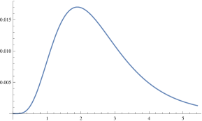
Figure 1: Plot of the function $\sigma_{K}^{2}(t),$

We find that

$$\sigma_{K}^{2}=\sup_{t\geq 0}\sigma_{K}^{2}(t)=0.017.$$

The supremum is reached for $t_{0}=1.892$. Therefore, our family of kernels $\Xi(X_{1},X_{2},X_{3},X_{4},t)$ is non-degenerate as defined in [21]. It can be shown (see [28]) that $U$-empirical process

$$\sqrt{n}\left(H_{n}(t)-G_{n}(t)\right),\ t\geq 0,$$

weakly converges in $D(0,\infty)$ as $n\to\infty$ to certain centered Gaussian process with calculable covariance. Thus, the sequence of our test statistic $K_{n}$ converges in distribution to the random variable $\sup_{t\geq 0}|\sqrt{n}\big{(}H_{n}(t)-G_{n}(t)\big{)}|$ but its distribution is unknown.

Critical values for statistics $K_{n}$ for different sample size and the level of significance are shown in the table 2. They are calculated using Monte Carlo methods based on 10000 repetitions.

Table 2: Critical values for statistics $K_{n}$

$n$	$\alpha=0.1$	$\alpha=0.05$	$\alpha=0.025$	$\alpha=0.01$
10	0.49	0.56	0.62	0.70
20	0.33	0.39	0.43	0.48
30	0.26	0.30	0.34	0.38
40	0.23	0.26	0.29	0.31
50	0.20	0.23	0.25	0.28
100	0.14	0.16	0.17	0.19

3.1 Local Bahadur efficiency

The family of kernels $\{\Xi_{4}(X_{1},X_{2},X_{3},X_{4},t),\;t\geq 0\}$ is centered and bounded in the sense described in [21]. Applying the large deviation theorem for the supremum of the family of non-degenerate $U$- and $V$-statistics from [21] , we find function $f$ from (5).

Lemma 3.1

For statistic $K_{n}$ the function $f_{K}$ from (5) is analytic for sufficiently small $\epsilon>0$ and it holds

$$f_{K}(\epsilon)=\frac{1}{32\sigma^{2}_{K}}\epsilon^{2}+o(\epsilon^{2})\approx 1.84\epsilon^{2}+o(\epsilon^{2}),\;\epsilon\rightarrow 0.$$

Lemma 3.2

For a given alternative density $g(x;\theta)$ whose distribution belongs to $\mathcal{G}$ holds

$$b_{K}(\theta)=4\theta\sup\limits_{t\geq 0}\big{|}\int_{0}^{\infty}\xi(x;t)h(x)dx\big{|}+o(\theta),\,\theta\to 0.$$

Using Glivenko-Cantelli theorem for $V$-statistics [10] we have

$$b_{K}(\theta) =\sup\limits_{t\geq 0}\big{|}P\{\max(X_{2},X_{3},X_{4})<t\}-P\{X_{1}+{\rm med}(X_{2},X_{3},X_{4})<t\}\big{|}$$ (23)

$$=\sup\limits_{t\geq 0}\big{|}G^{3}(t,\theta)-6\int\limits_{0}^{t}g(x,\theta)\int\limits_{0}^{t-x}G(y,\theta)(1-G(y,\theta))g(y,\theta)dydx\big{|}.$$

Denote

$$a(t,\theta)=G^{3}(t,\theta)-6\int\limits_{0}^{t}g(x,\theta)\int\limits_{0}^{t-x}G(y,\theta)(1-G(y,\theta))g(y,\theta)dydx.$$ (24)

Performing calculations similar to those from lemma 2.2 we get

$$a_{\theta}^{\prime}(t,0) =\int\limits_{0}^{t}h(x)(4\xi(x,t)+e^{-3t}(1-6e^{t}+2e^{3t}+e^{2t}(3-6t))dx$$

$$=4\int\limits_{0}^{\infty}h(x)\xi(x,t)dx.$$

Expanding $a(t,\theta)$ in Maclaurin series and inserting the result in (23) we get the statement of the lemma.

Now we shall calculate the local Bahadur efficiencies in the same manner as we did for integral-type statistic. For the alternatives (13) and (17) the process of calculations is presented in following two examples, while for the others the values of efficiencies are presented in table 3.

Example 3.3

Let the alternative hypothesis be Weibull distribution with density function (13). Using lemma 3.2 we have

$$a(t,\theta)=4\theta\int_{0}^{\infty}\xi(x,t)(e^{-x}+e^{-x}\log x-e^{-x}x\log x)dx+o(\theta),\;\;\theta\to 0.$$ (25)

The plot of the function function $a_{\theta}^{\prime}(t,0)$, is shown in figure 2.

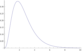
Figure 2: Plot of the function $a_{\theta}^{\prime}(t,0)$

Supremum of $a(t,\theta)$ is reached at $t_{1}=1.761$, thus $b_{K}(\theta)=0.34\theta+o(\theta),\;\;\theta\to 0$.

Using lemma 3.1 and equations (6) and (8) we get that the local Bahadur efficiency in case of statistic $K_{n}$ is 0.258.

Example 3.4

Let the alternative density function be (17). The function $a(t,\theta)$ from (24) is equal to

$$a(t,\theta) =\frac{3}{4(1+\theta)^{4}}e^{-3t}\theta^{2}\big{(}-2-8\theta-9\theta^{2}-2t^{3}\theta^{2}-4t^{2}\theta(1+2\theta)$$

$$+8e^{t}(1+\theta)(2+t+6\theta+4t\theta+t^{2}\theta)-t(2+10\theta+13\theta^{2})$$

$$+e^{2t}(-14-56\theta-39\theta^{2}+t(6+18\theta+11\theta^{2}))\big{)}$$

$$=\frac{3}{2}(-e^{-3t}+8e^{-2t}-7e^{-t}-te^{-3t}+4e^{-2t}t+3e^{-t}t)\theta^{2}+o(\theta^{2}).$$

The plot of the function $a_{2}(t)$, the coefficient next to $\theta^{2}$, in the expression above is given in figure 3. Thus we have

$$\sup_{t\geq 0}|a(t,\theta)|=0.241\theta^{2}+o(\theta^{2}),\;\theta\to 0.$$

The value of double Kullback-Leibler distance is given in (18). Using lemma 3.1 and equations (6) and (8) we get that the local Bahadur efficiency is 0.213.

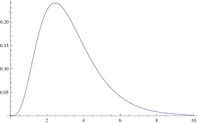
Figure 3: Plot of the function $a_{2}(t)$

Table 3: Local Bahadur efficiency for the statistic $K_{n}$

Alternative	Efficiency
Weibull	0.258
Makeham	0.370
EMNW(3)	0.364
GED	0.298
EE	0.213

We can see that, as expected, the efficiencies are lower than in case of the integral-type test. However the efficiencies are not that bad compared to some other Kolmogorov-type tests based on characterizations (e. g. [29]).

3.2 Locally optimal alternatives

In this section we derive one class of alternatives that are locally optimal for test based on statistic $K_{n}$.

Theorem 3.5

Let $g(x;\theta)$ be the density from $\mathcal{G}$ that satisfies condition

$$\int\limits_{0}^{\infty}e^{x}h^{2}(x)dx<\infty.$$ (26)

Alternative densities

$$g(x;\theta)=e^{-x}+e^{-x}\theta(C\xi(x,t_{0})+D(x-1)),\;x\geq 0,\;C>0,\;D\in\mathbb{R},$$

where $t_{0}=1.892$, are for small $\theta$ locally asymptotically optimal for the test based on $K_{n}$.

Proof. We use function $h_{0}$ defined in (20). It can be shown that function $h_{0}$ satisfies the condition (21) and

$$\int\limits_{0}^{\infty}\xi(x)h_{0}(x)dx=\int\limits_{0}^{\infty}\xi(x)h(x)dx.$$

Local asymptotic efficiency is

$$e_{K} =\lim\limits_{\theta\rightarrow 0}\frac{c_{K}(\theta)}{2K(\theta)}=\lim\limits_{\theta\rightarrow 0}\frac{2f(b_{K}(\theta))}{2K(\theta)}==\lim\limits_{\theta\rightarrow 0}\frac{b_{K}^{2}(\theta)}{16\sigma_{K}(t_{0})^{2}2K(\theta)}$$

$$=\lim\limits_{\theta\rightarrow 0}\frac{16\theta^{2}\sup\limits_{t\geq 0}\bigg{(}\int\limits_{0}^{\infty}\xi(x,t)h(x)dx\bigg{)}^{2}+o(\theta^{2})}{16\sup\limits_{t\geq 0}\int\limits_{0}^{\infty}\xi^{2}(x,t)e^{-x}dx\bigg{(}\theta^{2}(\int\limits_{0}^{\infty}e^{x}h^{2}(x)dx-\big{(}\int\limits_{0}^{\infty}h(x)xdx\big{)}^{2})+o(\theta^{2})\bigg{)}}$$

$$=\frac{\sup\limits_{t\geq 0}\bigg{(}\int\limits_{0}^{\infty}\xi(x,t)h(x)dx\bigg{)}^{2}}{\sup\limits_{t\geq 0}\int\limits_{0}^{\infty}\xi^{2}(x,t)e^{-x}dx\bigg{(}\int\limits_{0}^{\infty}e^{x}h^{2}(x)dx-\big{(}\int\limits_{0}^{\infty}h(x)xdx\big{)}^{2}\bigg{)}}$$

$$=\frac{\sup\limits_{t\geq 0}\bigg{(}\int\limits_{0}^{\infty}\xi(x,t)h_{0}(x)dx\bigg{)}^{2}}{\int\limits_{0}^{\infty}\xi^{2}(x,t)e^{-x}dx\int\limits_{0}^{\infty}h^{2}_{0}(x)e^{x}dx}.$$

From the Cauchy-Schwarz inequality we have that $e_{K}=1$ if and only if $h_{0}(x)=C\xi(x,t_{0})e^{-x}$. Inserting that in (20) we obtain $h(x)$. The densities from the statement of the theorem have the same $h(x)$, hence the proof is completed. $\hfill\Box$

4 Power comparison

For purpose of comparison we calculated the powers for sample sizes $n=20$ and $n=50$ for some common distributions and compare results with some other tests for exponentiality which can be found in [11]. The powers are shown in tables 4 and 5. The labels used are identical to the ones in [11]. Bolded numbers represent cases where our test(s) have the higher or equal power than the competitors tests. It can be noticed that in majority of cases statistic $I_{n}$ is the most powerful. Statistic $K_{n}$ also in most cases performs better than the competitor tests for $n=20$, while it is reasonably competitive for $n=50$. However there are few cases where the powers of both our tests are unsatisfactory.

5 Application to real data

This data set represents inter-occurrence times of fatal accidents to British registered passenger aircraft, 1946-63, measured in number of days and listed in the order of their occurrence in time (see [27]):

20 106 14 78 94 20 21 136 56 232 89 33 181 424 14430 155 205 117 253 86 260 213 58 276 263 246 341 1105 50 136.

Applying our tests to these data, we get the following values of test statistics $I_{n}$ and $K_{n}$, as well as the corresponding p-values:

statistic	$I_{n}$	$K_{n}$
value	0.04	0.21
p-value	0.32	0.24

so we conclude that the tests do not reject exponentiality.

Table 4: Percentage of significant samples for different exponentiality tests $n=20$, $\alpha=0.05$

Alternative	$EP$	$\overline{KS}$	$\overline{CM}$	$\omega^{2}$	$KS$	$KL$	$S$	$CO$	$I$	$K$
W(1.4)	36	35	35	34	28	29	35	37	46	32
$\Gamma(2)$	48	46	47	47	40	44	46	54	59	32
LN(0.8)	25	28	27	33	30	35	24	33	9	6
HN	21	24	22	21	18	16	21	19	30	25
U	66	72	70	66	52	61	70	50	79	89
CH(0.5)	63	47	61	61	56	77	63	80	23	20
CH(1.0)	15	18	16	14	13	11	15	13	22	19
CH(1.5)	84	79	83	79	67	76	84	81	22	20
LF(2.0)	28	32	30	28	24	23	29	25	39	32
LF(4.0)	42	44	43	41	34	34	42	37	53	44
EW(0.5)	15	18	16	14	13	11	15	13	22	19
EW(1.5)	45	48	47	43	35	37	46	37	57	52

Table 5: Percentage of significant samples for different exponentiality tests $n=50$, $\alpha=0.05$

Alternative	$EP$	$\overline{KS}$	$\overline{CM}$	$\omega^{2}$	$KS$	$KL$	$S$	$CO$	$I$	$K$
W(1.4)	80	71	77	75	64	72	79	82	82	62
$\Gamma(2)$	91	86	90	90	83	93	90	96	94	72
LN(0.8)	45	62	60	76	71	92	47	66	14	7
HN	54	50	53	48	39	37	54	45	58	50
U	98	99	99	98	93	97	99	91	99	100
CH(0.5)	94	90	94	95	92	99	94	99	41	37
CH(1.0)	38	36	37	32	26	23	38	30	41	38
CH(1.5)	100	100	100	100	98	100	100	100	40	38
LF(2.0)	69	65	69	64	53	54	69	60	73	62
LF(4.0)	87	82	87	83	72	75	87	80	88	79
EW(0.5)	38	36	37	32	26	23	38	30	41	37
EW(1.5)	90	88	90	86	75	79	90	78	90	88

6 Conclusion

In this paper two goodness of fit tests based on a characterization were studied. The major advantage of our tests is that they are free of parameter $\lambda$. The local Bahadur efficiencies for some alternatives were calculated and the results are more than satisfactory. For both tests locally optimal class of alternatives were determined. These tests were compared with other goodness-of-fit tests and it can be noticed that in most cases our tests are more powerful.

References

- [1]
- [2] I. Ahmad, I. Alwasel, A goodness-of-fit test for exponentiality based on the memoryless property. J. Roy. Statist. Soc. 61, Pt.3 (1999), 681 – 689.
- [3] M. Ahsanullah, G. G. Hamedani. Exponential Distribution: Theory and Methods. NOVA Science, New York, 2010.
- [4] B.C. Arnold, N. Balakrishnan, H.N. Nagaraja, A First Course in Order Statistics, SIAM, Philadelphia, 2008.
- [5] J. E. Angus, Goodness-of-fit tests for exponentiality based on a loss-of-memory type functional equation. J. Statist. Plann. Infer. 6 (1982), 241 – 251.
- [6] R. R. Bahadur, Some limit theorems in statistics. SIAM, Philadelphia, 1971.
- [7] N. Balakrishnan, C.R. Rao, Order Statistics, Theory & Methods, Elsevier, Amsterdam, 1998.
- [8] J. Galambos, S. Kotz, Characterizations of Probability Distributions, Berlin-Heidelberg-New York, Springer-Verlag, (1978)
- [9] Y.M. Gomez, H. Bolfarine, H.W. Gomez, A New Extension of the Exponential Distribution, Revista Colombiana de Estad stica, , 37(1) (2014), 25–34.
- [10] R. Helmers, P. Janssen, R. Serfling, Glivenko-Cantelli properties of some generalized empirical DF’s and strong convergence of generalized L-statistics. Probab. Theory Relat. Fields 79 (1988), 75 – 93.
- [11] N. Henze, S.G Meintanis, Recent and clasicical tests for exponentiality:A partial review with comparisons, Metrika, 61(1) (2005),29-45.
- [12] W. Hoeffding, A class of statistics with asymptotically normal distribution. Ann. Math. Statist., 19 (1948), 293 – 325.
- [13] H.M. Jansen Van Rensburg, J.W.H. Swanepoel. A class of goodness-of-fit tests based on a new characterization of the exponential distribution. J. of Nonparam. Stat., 20(2008), N 6, 539 – 551.
- [14] V. Jevremović, A note on mixed exponential distribution with negative weights. Stat. Probabil. Lett. 11(3) (1991), 259-265.
- [15] V. S. Korolyuk, Yu. V. Borovskikh, Theory of -statistics. Kluwer, Dordrecht, 1994.
- [16] H. L. Koul, A test for new better than used. Commun. Statist. Theory and Meth.6 (1977), 563 – 574.
- [17] H. L. Koul, Testing for new is better than used in expectation. Commun. Statist. Theory and Meth. 7 (1978), 685 – 701.
- [18] S. Nadarajah, F. Haghigni, An extension of the exponential distribution, Statistics: A Journal of Theoretical and Applied Statistics, (45(6)) (2010) 543-558.
- [19] Y. Nikitin, Asymptotic efficiency of nonparametric tests. Cambridge University Press, New York, 1995.
- [20] Ya. Yu. Nikitin. Bahadur efficiency of a test of exponentiality based on a loss of memory type functional equation. J. Nonparam. Stat 6(1996), N 1, 13 - 26.
- [21] Ya. Yu. Nikitin, Large deviations of -empirical Kolmogorov-Smirnov tests, and their efficiency. J. Nonparam. Stat., 22 (2010), 649 – 668.
- [22] Ya. Yu. Nikitin, Local Asymptotic Bahadur Optimality and Characterization Problems, Probability Theory and its Applications, 29(1984), 79-92.
- [23] M. Obradović, Three Characterizations of Exponential Distribution Involving the Median of Sample of Size Three, arXiv:1412.2563 (2014)
- [24] Ya. Yu. Nikitin, E. V. Ponikarov, Rough large deviation asymptotics of Chernoff type for von Mises functionals and -statistics. Proc. of St.Petersburg Math. Society 7 (1999), 124–167. Engl. transl. in AMS Transl., ser.2 203(2001), 107 – 146.
- [25] Ya. Yu. Nikitin, A. V. Tchirina, Bahadur efficiency and local optimality of a test for the exponential distribution based on the Gini statistic. Statist. Meth. and Appl., 5 (1996), 163 – 175.
- [26] Ya. Yu. Nikitin, K. Yu. Volkova, Asymptotic efficiency of exponentiality tests based on order statistics characterization. Georgian Math. Journ., 17 (2010), 749 – 763.
- [27] R. Pyke, Spacings, J Roy Stat Soc B Met 27(3) (1965), 395 – 449.
- [28] B. W. Silverman, Convergence of a class of empirical distribution functions of dependent random variables. Ann. Probab. 11(1983), 745 – 751.
- [29] K.Y. Volkova, On asymptotic efficiency of exponentiality tests based on Rossbergs characterization, J. Math. Sci. (N.Y.) 167(4) (2010), 486–494.
- [30] H. S. Wieand, A condition under which the Pitman and Bahadur approaches to efficiency coincide. Ann. Statist. 4 (1976), 1003 – 1011.