Potential description of the charmonium from lattice QCD

Abstract

We present spin-independent and spin-spin interquark potentials for charmonium states, that are calculated using a relativistic heavy quark action for charm quarks on the PACS-CS gauge configurations generated with the Iwasaki gauge action and 2+1 flavors of Wilson clover quark. The interquark potential with finite quark masses is defined through the equal-time Bethe-Salpeter amplitude. The light and strange quark masses are close to the physical point where the pion mass corresponds to $M_{\pi}\approx 156(7)$ MeV, and charm quark mass is tuned to reproduce the experimental values of $\eta_{c}$ and $J/\psi$ states. Our simulations are performed with a lattice cutoff of $a^{-1}\approx 2.2$ GeV and a spatial volume of $(3~{}{\rm fm})^{3}$. We solve the nonrelativistic Schrödinger equation with resulting charmonium potentials as theoretical inputs. The resultant charmonium spectrum below the open charm threshold shows a fairly good agreement with experimental data of well-established charmonium states.

1 Introduction

The heavy-quark ($Q$)-antiquark ($\overline{Q}$) potential is an important quantity to understand many properties of the heavy quarkonium states. The dynamics of heavy quarks can be described well within the framework of nonrelativistic quantum mechanics, because of their masses being much larger than the QCD scale ($\Lambda_{\rm QCD}$). Indeed the constituent quark potential models with a QCD-motivated $Q\overline{Q}$ potential have successfully reproduced the heavy quarkonium spectra and also decay rates below open thresholds Eichten et al. (1975); Godfrey and Isgur (1985); Barnes et al. (2005).

In the nonrelativistic potential (NRp) models, the heavy quarkonium states such as charmonium and bottomnium are well understood as is a quark-antiquark pair bound by the Coulombic induced by perturbative one-gluon exchange, plus linearly rising potential. The former dominates in short range, while the latter describes the phenomenology of confining quark interactions at large distances Eichten et al. (1975). This potential is called as Cornell potential and its functional form is given by $V(r)=-\frac{4}{3}\frac{\alpha_{s}}{r}+\sigma r+V_{0}$ where $\alpha_{s}$ and $\sigma$ denote the strong coupling constant and the string tension, and $V_{0}$ is the constant term associated with a self-energy contribution of the color sources. In the NRp models, spin-dependent potentials are induced as relativistic corrections in powers of the relative velocity of quarks, and their functional forms are also determined on the basis of perturbative one-gluon exchange as the Fermi-Breit type potential Eichten and Feinberg (1981). However the validity of the phenomenological spin-dependent potentials determined within the perturbative method would be limited only at short distances and also in the vicinity of the heavy quark mass limit. This may cause large uncertainties in the predictions for higher heavy quarkonium states obtained in the NRp models.

Lattice QCD simulations offer a strong tool to understand the properties of $Q\overline{Q}$ interactions. Indeed, both the static $Q\overline{Q}$ potential and its corrections of order $\mathcal{O}(1/m_{Q}^{2})$ as the spin dependent potentials have been precisely determined from Wilson loops using lattice QCD simulations with the multilevel algorithm Koma and Koma (2007, 2010). Although the lattice QCD calculations within the Wilson loop formalism support a shape of the Cornell potential Bali (2001), the leading spin-spin potential determined at $\mathcal{O}(1/m_{Q}^{2})$ gives an attractive interaction for the higher spin states Bali et al. (1997a, b), in contradiction with a repulsive one that is demanded by phenomenological analysis. The higher order corrections beyond the next-to-leading order are required to correctly describe the conventional charmonium spectrum, because the inverse of the charm quark mass would be far outside the validity region of the $1/m_{Q}$ expansion Kawanai and Sasaki (2014). In addition, practically, the multilevel algorithm is quite difficult to be implemented in dynamical lattice QCD simulations.

Under this situation, we employ the new method proposed in our previous works Kawanai and Sasaki (2014, 2011, 2012) in order to obtain the proper interquark potentials fitted in the NRp models. The interquark potential and also the quark kinetic mass are defined by the equal-time and Coulomb gauge Bethe-Salpeter (BS) amplitude through an effective Schrödinger equation. This new method enables us to determine the interquark potentials including spin-dependent terms at finite quark masses from first principles of QCD, and then can fix all parameters that are needed in the NRp models. Furthermore, there is no restriction to extend to the dynamical calculations. Hereafter we call the new method as BS amplitude method.

Once we obtain the reliable $Q\overline{Q}$ potentials from lattice QCD, we can solve the nonrelativistic Schrödinger equation with “lattice-determined potentials” as theoretical inputs, and obtain many physical observables such as mass spectrum. In this proceedings, we present not only the charmonium potentials calculated with almost physical quark masses using the $2+1$ flavor PACS-CS gauge configurations Aoki et al. (2009), but also the resultant charmonium mass spectrum computed from the NRp model with the lattice-determined potentials, where there are no free parameters including the $V_{0}$ and quark mass. The simulated pion mass $M_{\pi}\approx 156(7)$ MeV is almost physical. For the heavy quarks, we employ the relativistic heavy quark action that can control large discretization errors introduced by large quark mass Aoki et al. (2003).

2 Formalism

In this section, we briefly review the BS amplitude method utilized to calculate the interquark potential with the finite quark mass. This is an application based on the approach originally used for studing the hadron-hadron potential, which is defined through the equal-time BS amplitude Ishii et al. (2007); Aoki et al. (2010). More details of determination of the interquark potential are given in Ref. Kawanai and Sasaki (2014).

In lattice simulations, we measure the following equal-time $Q\overline{Q}$ BS amplitude in the Coulomb gauge for the quarkonium states Velikson and Weingarten (1985); Gupta et al. (1993):

$$\phi_{\Gamma}({\bf r})=\sum_{{\bf x}}\langle 0|\overline{Q}({\bf x})\Gamma Q({\bf x}+{\bf r})|Q\overline{Q};J^{PC}\rangle,$$ (1)

where ${\bf r}$ is the relative coordinate between quark and antiquark at time slice $t$. The Dirac $\gamma$ matrices $\Gamma$ in Eq. (1) specify the spin and the parity of meson states. For instance, $\gamma_{5}$ and $\gamma_{i}$ correspond to the pseudoscalar (PS) and the vector (V) channels with $J^{PC}=0^{-+}$ and $J^{PC}=1^{--}$, respectively. A summation over spatial coordinates ${\bf x}$ projects onto zero total momentum. The ${\bf r}$-dependent amplitude, $\phi_{\Gamma}({\bf r})$, is here called BS wave function. The BS wave function can be extracted from four-point correlation function at large time separation. Also, the corresponding meson masses $M_{\Gamma}$ can be read off from the asymptotic large-time behavior of two-point correlation functions. In this proceedings, we focus only on the $S$-wave charmonium states ($\eta_{c}$ and $J/\psi$), obtained by appropriate projection to the $A^{+}_{1}$ representation in cubic group Luscher (1991).

The BS wave function satisfies an effective Schrödinger equation with a nonlocal and energy-independent interquark potential $U$ Ishii et al. (2007); Caswell and Lepage (1978); Ikeda and Iida (2012)

$$-\frac{\nabla^{2}}{2\mu}\phi_{\Gamma}({\bf r})+\int dr^{\prime}U({\bf r},{\bf r}^{\prime})\phi_{\Gamma}({\bf r}^{\prime})=E_{\Gamma}\phi_{\Gamma}({\bf r}),$$ (2)

where $\mu$ is the reduced mass of the $Q\overline{Q}$ system. The energy eigenvalue $E_{\Gamma}$ of the stationary Schrödinger equation is supposed to be $M_{\Gamma}-2m_{Q}$. If the relative quark velocity $v=|{\nabla}/m_{Q}|$ is small as $v\ll 1$, the nonlocal potential $U$ can generally expand in terms of the velocity $v$ as $U({\bf r}^{\prime},{\bf r})=\{V(r)+V_{\text{S}}(r){\mathbf{S}}_{Q}\cdot{\mathbf{S}}_{\overline{Q}}+V_{\text{T}}(r)S_{12}+V_{\text{LS}}(r){\bf L}\cdot{\bf S}+\mathcal{O}(v^{2})\}\delta({\bf r}^{\prime}-{\bf r})$ where $S_{12}=({\mathbf{S}}_{Q}\cdot\hat{r})({\mathbf{S}}_{\overline{Q}}\cdot\hat{r})-{\mathbf{S}}_{Q}\cdot{\mathbf{S}}_{\overline{Q}}/3$ with $\hat{r}={\bf r}/r$, ${\bf S}={\mathbf{S}}_{Q}+{\mathbf{S}}_{\overline{Q}}$ and ${\bf L}={\bf r}\times(-i\nabla)$ Ishii et al. (2007). Here, $V$, $V_{\text{S}}$, $V_{\text{T}}$ and $V_{\text{LS}}$ represent the spin-independent central, spin-spin, tensor and spin-orbit potentials, respectively.

The Schrödinger equation for $S$-wave is simplified as

$$\left\{-\frac{\nabla^{2}}{m_{Q}}+V(r)+{\mathbf{S}}_{Q}\cdot{\mathbf{S}}_{\overline{Q}}V_{\text{S}}(r)\right\}\phi_{\Gamma}(r)=E_{\Gamma}\phi_{\Gamma}(r)$$ (3)

at the leading order of the $v$-expansion. Here, we essentially follow the NRp models, where the $J/\psi$ state is purely composed of the $1S$ wave function.

The spin operator ${\mathbf{S}}_{Q}\cdot{\mathbf{S}}_{\overline{Q}}$ can be easily replaced by expectation values $-3/4$ and $1/4$ for the PS and V channels, respectively. Then, the spin-independent and spin-spin $Q\overline{Q}$ potentials can be evaluated through the following linear combinations of Eq.(3):

$$V(r) = E_{\text{ave}}+\frac{1}{m_{Q}}\left\{\frac{3}{4}\frac{\nabla^{2}\phi_{\text{V}}(r)}{\phi_{\text{V}}(r)}+\frac{1}{4}\frac{\nabla^{2}\phi_{\text{PS}}(r)}{\phi_{\text{PS}}(r)}\right\}$$ (4)

$$V_{\text{S}}(r) = E_{\text{hyp}}+\frac{1}{m_{Q}}\left\{\frac{\nabla^{2}\phi_{\text{V}}(r)}{\phi_{\text{V}}(r)}-\frac{\nabla^{2}\phi_{\text{PS}}(r)}{\phi_{\text{PS}}(r)}\right\},$$ (5)

where $E_{\text{ave}}=M_{\text{ave}}-2m_{Q}$ and $E_{\text{hyp}}=M_{\text{V}}-M_{\text{PS}}$. The mass $M_{\text{ave}}$ denotes the spin-averaged mass as $\frac{1}{4}M_{\text{PS}}+\frac{3}{4}M_{\text{V}}$. The derivative $\nabla^{2}$ is defined by the discrete Laplacian.

The kinetic quark mass is an important quantity in the determination of the interquark potentials since Eqs. (4) and (5) require an information of the kinetic quark mass $m_{Q}$. In our previous work Kawanai and Sasaki (2014, 2011, 2012), we propose to calculate the quark kinetic mass through the large-distance behavior in the spin-spin potential with the help of the measured hyperfine splitting energy of $1S$ states in heavy quarkonia. Under a simple, but reasonable assumption as $\lim_{r\to\infty}V_{S}(r)=0$ which implies there is no long-range correlation and no irrelevant constant term in the spin-spin potential, Eq. (5) is rewritten as

$$m_{Q}=\lim_{r\to\infty}\frac{-1}{E_{\text{hyp}}}\left\{\frac{\nabla^{2}\phi_{\text{V}}(r)}{\phi_{\text{V}}(r)}-\frac{\nabla^{2}\phi_{\text{PS}}(r)}{\phi_{\text{PS}}(r)}\right\},$$ (6)

and then we can estimate the kinetic quark mass from asymptotic behavior of Eq. (6) in long range region.

3 Lattice setup

Table 1: Parameters of $2+1$-flavor dynamical QCD gauge field configurations generated by PACS-CS collaboration Aoki et al. (2009). The columns list number of flavors, lattice volume, the $\beta$ value, hopping parameters (light, strange), approximate lattice spacing (lattice cut-off), spatial physical volume, pion mass, number of configurations to be analyzed.

$N_{f}$	$L^{3}\times T$	$\beta$	$\kappa_{ud}$	$\kappa_{s}$	$a$ [fm] ($a^{-1}$ [GeV])	$La$ [fm]	$M_{\pi}$ [MeV]	# configs.
$2+1$	$32^{3}\times 64$	1.9	0.13781	0.13640	$\approx$ 0.0907 ($\approx$ 2.176)	$\approx$ 2.90	$\approx$156	198

The computation of the charmonium potential in this study is performed on a lattice $L^{3}\times T=32^{3}\times 64$ using the $2+1$ flavor PACS-CS gauge configurations Aoki et al. (2009) generated by non-perturbatively $\mathcal{O}(a)$-improved Wilson quark action with $c_{SW}=1.715$ Aoki et al. (2006) and Iwasaki gauge action at $\beta=1.90$ Iwasaki (1983), which corresponds to a lattice cutoff of $a^{-1}=2.176(31)$ GeV ($a=0.0907(13)$fm). The spatial lattice size then corresponds to $La\approx 3\;{\rm fm}$. The hopping parameters for the light sea quarks {$\kappa_{ud}$,$\kappa_{s}$}={0.13781, 0.13640} provide $M_{\pi}=156(7)$ MeV and $M_{K}=554(2)$ MeV Aoki et al. (2009). Table 1 summarizes simulation parameters of dynamical QCD simulations used in this work. Although the light sea quark masse is slightly off the physical point, the systematic uncertainty due to this fact could be extremely small in this project. Our results are analyzed on all 198 gauge configurations. All gauge configurations are fixed to Coulomb gauge.

Table 2: The hopping parameter $\kappa_{Q}$ and RHQ parameters used for the charm quark.

$\kappa_{c}$	$\nu$	$r_{s}$	$c_{B}$	$c_{E}$
0.10819	1.2153	1.2131	2.0268	1.7911

In order to control discretization errors induced by large quark mass, we employ the relativistic heavy quark (RHQ) action Aoki et al. (2003) that removes main errors of $\mathcal{O}(|\vec{p}|a)$, $\mathcal{O}((m_{0}a)^{n})$ and $\mathcal{O}(|\vec{p}|a(m_{0}a)^{n})$ from on-shell Green’s functions. The RHQ action is the anisotropic version of the $\mathcal{O}(a)$ improved Wilson action with five parameters $\kappa_{c}$, $\nu$, $r_{s}$, $c_{B}$ and $c_{E}$, called RHQ parameters (for more details see Ref. Aoki et al. (2003); Kayaba et al. (2007)). The RHQ action utilized here is a variant of the Fermilab approach El-Khadra et al. (1997) (See also Ref. Christ et al. (2007)).

The parameters $r_{s}$, $c_{B}$ and $c_{E}$ in RHQ action are determined by tadpole improved one-loop perturbation theory Kayaba et al. (2007). For $\nu$, we use a nonperturbatively determined value, which is adjusted by reproducing the effective speed of light $c_{\text{eff}}$ to be unity in the dispersion relation $E^{2}({\bf p}^{2})=M^{2}+c^{2}_{\text{eff}}|{\bf p}|^{2}$ for the spin-averaged $1S$-charmonium state, since the parameter $\nu$ is sensitive to the size of hyperfine splitting energy Namekawa et al. (2011). We choose $\kappa_{c}$ to reproduce the experimental spin-averaged mass of $1S$-charmonium states $M_{\text{ave}}^{\text{exp}}(1S)=3.0678(3)$ GeV. To calibrate adequate RHQ parameters, we employ a gauge invariant Gauss smearing source for the standard two-point correlation function with four finite momenta. As a result, the relevant speed of light in the dispersion relation is consistent with unity within statistical error: $c^{2}_{\text{eff}}=1.04(5)$. Our chosen RHQ parameters are summarized in Table 2.

Using tuned RHQ parameters, we compute two valence quark propagators with wall sources located at different time slices $t_{\rm s}/a=6$ and $57$ to increase statistics. Two sets of two and four-point correlation functions are constructed from the corresponding quark propagators, and folded together to create the single correlation function. Dirichlet boundary condition is imposed for the time direction to eliminate unwanted contributions across time boundaries.

state ($J^{PC}$)	fit range	mass [GeV]	$\chi^{2}/{\rm d.o.f.}$
$\eta_{c}$ ($0^{-+}$)	[33:47]	2.9851(5)	0.70
$J/\psi$ ($1^{-+}$)	[33:47]	3.0985(11)	0.62
$\chi_{c0}$ ($0^{++}$)	[14:26]	3.3928(59)	0.66
$\chi_{c1}$ ($1^{++}$)	[14:26]	3.4845(62)	1.03
$h_{c}$ ($1^{+-}$)	[14:26]	3.5059(62)	0.63
$M_{\text{ave}}(1S)$	-	3.0701(9)	-
$E_{\text{hyp}}(1S)$	-	0.1138(8)	-

Table 3: Masses of low-lying charmonium states calculated from two-point functions, the spin-averaged mass and hyperfine splitting energy of $1S$ charmonium states. The fitting ranges and values of $\chi^{2}/{\rm d.o.f.}$ are also included. Results are shown in units of GeV.

Low-lying charmonium masses of $\eta_{c}$, $J/\psi$, $h_{c}$, $\chi_{c0}$ and $\chi_{c1}$ are obtained by weighted average of the effective mass in the appropriate range. The effective mass is defined as

$$M_{\Gamma}(t)=\log\frac{G_{\Gamma}(t,t_{\rm s})}{G_{\Gamma}(t+1,t_{\rm s})},$$ (7)

where $G_{\Gamma}(t,t_{\rm s})$ is a two-point function obtained by setting ${\bf r}$ to be zero in four-point function $G_{\Gamma}({\bf r},t,t_{\rm s})$. In Table 2, we summarize resultant charmonium masses together with fit ranges used in the fits and $\chi^{2}/{\rm d.o.f.}$ values. We take into account a correlation between effective masses measured at various time slices in the fit. The statistical errors are estimated by the jackknife method.

Low-lying charmonium masses calculated in this study below $D\bar{D}$ threshold are all close to the experimental values, though the hyperfine mass splitting $M_{\text{hyp}}=0.1124(9)$ GeV is slightly smaller than the experimental value, $M_{\text{hyp}}^{\text{exp}}=0.1166(12)$ GeV Beringer et al. (2012). Note that here we simply neglect the disconnected diagrams in two-point correlation functions. The several numerical studies reported that the contributions of charm annihilation to the hyperfine splitting of the $1S$-charmonium state are sufficiently small, as of order $1-4$ MeV. McNeile and Michael (2004); de Forcrand et al. (2004); Levkova and DeTar (2011),

4 Determination of interquark potential

4.1 $Q\overline{Q}$ BS wave function

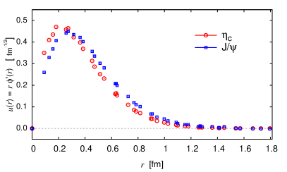
Figure 1: The reduced $Q\overline{Q}$ BS wave functions of the $\eta_{c}$ (circles) and $J/\psi$ (squares) states, shown as a function of the spatial distance $r$. The data points are taken along $\bf r$ vectors which are multiples of three directions $(1,0,0)$, $(1,1,0)$ and $(1,1,1)$.

Fig. 1 shows the $Q\overline{Q}$ BS wave functions of $1S$ charmonium states ($\eta_{c}$ and $J/\psi$ states). The BS wave functions are defined by Eq.(1) and normalized as $\sum\phi_{\Gamma}^{2}=1$. We use the reduced wave function $u_{\Gamma}(r)$ for displaying the wave function: $u_{\Gamma}(r)=r\phi_{\Gamma}({\bf r})$. Practically we take average of the BS wave function by weight over time slices $33\leq t/a\leq 47$ where effective mass plots for $1S$-charmonium states show plateaus and excited state contaminations are expected to be negligible. In Fig. 1 we display data points of $u_{\Gamma}(r)$ calculated at $\bf r$ vectors which are multiples of $(1,0,0)$, $(1,1,0)$ and $(1,1,1)$. Hereafter we focus on lattice data taken in three directions for any quantities.

We find that a sign of rotational symmetry breading found in the $Q\overline{Q}$ BS wave functions is sufficiently small in our calculation. The resulting wave functions become isotropic with the help of a projection to the $A_{1}^{+}$ sector of the cubic group that corresponds to the $S$-wave in the continuum theory (Fig. 1).

4.2 quark kinetic mass

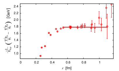
Figure 2: The determination of quark kinetic mass within the BS amplitude method. The values of $-(\nabla^{2}\phi_{V}/\phi_{V}-\nabla^{2}\phi_{P}/\phi_{P})/E_{\text{hyp}}$ as a function of the spatial distance $r$ are shown in this figure. The quark kinetic mass $m_{Q}$ is obtained from the long-distance asymptotic values of $-(\nabla^{2}\phi_{V}/\phi_{V}-\nabla^{2}\phi_{P}/\phi_{P})/E_{\text{hyp}}$. Horizontal solid line indicates a value of quark kinetic mass obtained by fitting a asymptotic constant in the range $0.54~{}\text{fm}\hskip 3.00003pt\raisebox{1.72218pt}{$<$}\raisebox{-3.01385pt}{$\sim$}\hskip 3.00003ptr\hskip 3.00003pt\raisebox{1.72218pt}{$<$}\raisebox{-3.01385pt}{$\sim$}\hskip 3.00003pt1.10~{}\text{fm}$. A shaded band indicates a statistical error estimated by estimated by jackknife method.

In our formalism, the kinetic mass of the charm quark is determined self-consistently within the BS amplitude method as well Kawanai and Sasaki (2011). The quark kinetic mass defined in Eq. (6) is calculated from asymptotic behavior of the quantity $-(\nabla^{2}\phi_{V}/\phi_{V}-\nabla^{2}\phi_{P}/\phi_{P})/E_{\text{hyp}}$ at long distances. Fig. 2 illustrates the determination of quark kinetic mass $m_{Q}$ for the charmonium system.

For the derivative, we use the discrete Laplacian operator $\nabla^{2}$ defined in polar coordinates as

$$\nabla_{\bf r}^{2}\phi_{\Gamma}(r)=\frac{2}{r}\frac{\phi_{\Gamma}(r+\tilde{a})-\phi_{\Gamma}(r-\tilde{a})}{2\tilde{a}}+\frac{\phi_{\Gamma}(r+\tilde{a})+\phi_{\Gamma}(r-\tilde{a})-2\phi_{\Gamma}}{\tilde{a}^{2}}$$

where $r$ is the absolute value of the relative distance as $r=|{\bf r}|$ and $\tilde{a}$ is a spacing between grid points along differentiate directions. In the on-axis $({\bf r}\propto(1,0,0))$ and the two off-axis directions (${\bf r}\propto(1,1,0)$ and $(1,1,1)$), the effective grid spacings correspond to $\tilde{a}=a,\sqrt{2}a,\sqrt{3}a$, respectively.

The differences of ratios $\nabla^{2}\phi_{\Gamma}/\phi_{\Gamma}$ at each ${\bf r}$ are obtained by a constant fit to the lattice data with a reasonable $\chi^{2}/{\rm d.o.f.}$ value over the range of time slices where two-point functions exhibit the plateau behavior ($33\leq t/a\leq 47$). Then the values of $m_{Q}$ are determined for each directions from asymptotic values of $-(\nabla^{2}\phi_{V}/\phi_{V}-\nabla^{2}\phi_{P}/\phi_{P})/E_{\text{hyp}}$ in the range of $6\leq r/a\leq 7\sqrt{3}$ where $V_{S}(r)$ should vanish. Finally we average them over three directions, and then obtain $m_{Q}=1.784(23)(6)(20)$ GeV. The first error is statistical, given by the jackknife analysis. In the second error, we quote a systematic uncertainty due to rotational symmetry breaking by taking the largest difference between the average value and individual ones obtained for specific directions. The third one represents the systematic uncertainties due to choice of $t_{\rm min}$ of the time range used in the fits. We vary $t_{\rm min}$ over range $33-41$ and then quote the largest difference from the preferred determination of $m_{Q}$.

4.3 Spin-independent interquark potential

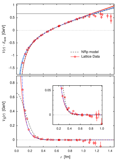
Figure 3: Central spin-independent and spin-spin charmonium potentials calculated from the BS wave functions in the dynamical QCD simulation with almost physical quark masses. In the upper panel, we show the spin-independent potential $V(r)$. A solid (dot-dashed) curve is the fit results with the Cornell (Cornell plus log) form. The shaded bands show statistical uncertainties in the fitting procedure where the jackknife analysis is used. Note that the spin-averaged eigen-energy of $1S$-charmonium state $E_{\rm ave}$ is not subtracted in this figure. A horizontal line indicates the level of open-charm ($D^{0}\bar{D}^{0}$) threshold $\approx 3729$ MeV. In the lower panel, we show the spin-spin potential $V_{S}(r)$. A solid (dot-dashed) curve corresponds to fitting results with exponential (Yukawa) form. The inset shows a magnified view. In both plots, the phenomenological potentials adopted in a NRp model Barnes et al. (2005) are also included as dashed curves for comparison.

Table 4: Summary of the Cornell parameters and the quark mass determined by the BS amplitude method. For comparison, ones adopted in a phenomenological NRp model Barnes et al. (2005) and ones of the static potential obtained from Polyakov line correlations are also included. In the first column, the quoted errors indicate the sum of the statistical and systematic added in quadrature.

	This work	Polyakov lines	NRp model
$A$	0.713(83)	0.476(81)	0.7281
$\sqrt{\sigma}$ [GeV]	0.402(15)	0.448(16)	0.3775
$m_{Q}$ [GeV]	1.784(31)	$\infty$	1.4794

Once the quark kinetic mass is determined, we can easily calculate the central spin-independent and spin-spin charmonium potentials from the $Q\bar{Q}$ BS wave function through Eqs. (4) and (5). First, we show a result of the spin-independent charmonium potential $V(r)$ in Fig. 3. The constant energy shift $E_{\rm ave}$ is not subtracted. At each distance ${\bf r}$, the values of interquark potentials $V(r)$ and $V_{S}(r)$ are practically determined by constant fits to data points over time slices where two-point functions exhibit the plateau behavior. The correlations between data points at different time slices are taken into account in the fitting process.

The charmonium potential calculated by the BS amplitude method from dynamical attice QCD simulations properly exhibits the linearly rising potential at large distances and the Coulomb-like potential at short distances. The finite $m_{Q}$ corrections could be encoded into the Cornell parameters, although the charm quark mass region would be beyond the radius of convergence for the systematic $1/m_{Q}$ expansion. Therefore, as first step, we simply adopt the Cornell parametrization to fit the data of the spin-independent central potential: $V(r)=-\frac{A}{r}+\sigma r+V_{0}$ with the Coulombic coefficient $A$, the string tension $\sigma$, and a constant $V_{0}$.

All fits are performed individually for each three directions over the range $[r_{\rm min}/a,r_{\rm max}/a]=[4:7\sqrt{3}]$. We minimize the $\chi^{2}/{\rm d.o.f}$ including the covariance matrix. Resulting Cornell parameters of the charmonium potential are $A=0.713(26)(38)(31)(62)$ and $\sqrt{\sigma}=0.402(6)(4)(9)(9)$ MeV with $\chi^{2}/\text{d.o.f.}\approx 3.2$. The first error is statistical and the second, third and forth ones are systematic uncertainties due to the choice of the differentiate direction, $t_{\rm min}$ and $r_{\min}$, respectively. The resulting Cornell parameters are summarized in Table 4. Also we include both phenomenological ones adopted in the NRp model Barnes et al. (2005) and of the static potential obtained from Polyakov loop correlations. The latter is calculated using the same method as in Ref. Aoki et al. (2009). Additionally we calculate the Sommer parameter defined as $r_{0}=\sqrt{(1.65-A)/\sigma}$, and then obtain $r_{0}=0.476(6)(11)(3)(6)$ fm, which is fairly consistent with the value quoted in Ref. Aoki et al. (2009).

As shown in Table 4, a gap for the Cornell parameters between the conventional static potential from Wilson-loops (Polyakov-loops) and the phenomenological potential used in the NRp models seems to be filled by our new approach, which nonperturbatively accounts for a finite quark mass effect. In the charmonium potential from the BS wave function, a Coulomb-like behavior is enhanced and the linearly rising force is slightly reduced due to finite charm quark mass effects. For the spin-independent central interquark potential, the $1/m_{Q}$ expansion within the Wilson-loop approach converges in the heavy quark mass region of $m_{Q}\hskip 3.00003pt\raisebox{1.72218pt}{$>$}\raisebox{-3.01385pt}{$\sim$}\hskip 3.00003pt1.8$ GeV. Indeed, as reported in Ref. Laschka et al. (2012), the static $Q\overline{Q}$ potential and its $1/m_{Q}$ corrections calculated in Ref. Koma et al. (2006) agree with the charmonium potential obtained from the BS amplitude method.

In order to provide a more adequate fit to the lattice data, we try to employ an alternative functional form adding a $\log$ term to the Cornell potential:

$$V(r)=-\frac{A}{r}+\sigma r+V_{0}+B\log(r\Lambda)$$ (8)

where $\Lambda$ is simply set to be lattice cutoff $a^{-1}$. Such $\log$ term as $1/m_{Q}$ corrections to the spin-independent potential is reported in Ref. Koma and Koma (2009). Resulting parameters are $A=0.194(137)(33)(36)(66)$, $\sqrt{\sigma}=0.300(38)(19)(20)(21)$ GeV and $B=0.390(113)(20)(39)(61)$ GeV. with $\chi^{2}/\text{d.o.f.}\approx 2.3$. Fitting range is determined to minimized a $\chi^{2}/\text{d.o.f.}$ value taking into account the correlation, and then we choose $[r_{\rm min}/a,r_{\rm max}/a]=[3:7\sqrt{3}]$.

The finite quark mass corrections to spin-independent potential give only a minor modification in the NRp models. In the upper panel of Fig. 3 the solid (dot-dashed) curve is given by the fitting the data to the Cornell form (Cornell plus log form). The phenomenological potential used in the NRp models Barnes et al. (2005) is also plotted as a dashed curve for comparison. The charmonium potential obtained from lattice QCD is similar to the one used in the NRp models, although a slope of the charmonium potential in the long range is barely larger than the phenomenological one.

It is worth mentioning that a string breaking-like behavior found in the range $r\hskip 3.00003pt\raisebox{1.72218pt}{$<$}\raisebox{-3.01385pt}{$\sim$}\hskip 3.00003pt1.1$ fm is unreliable. In principle, string breaking due to the presence of dynamical quarks is likely to be observed. The signal-to-noise ratio however becomes worse rapidly for the spin-independent potential as spatial distance $r$ increase because of the localized wave function. The lattice data of the potential near the spatial boundary are also sensitive to finite volume effects. Therefore, at least, calculations of the higher charmonium near the open charm threshold using a larger lattice are required for observing the string breaking. Their wave functions are extended until the string breaking sets in.

4.4 Spin-Spin potential

Table 5: Results of fitted parameters for the spin-spin potential with the exponential and Yukawa forms. The quoted errors are statistical only. In the case of the spin-spin potential, we use only on-axis data.

Functional form	$\alpha$	$\beta$	$\chi^{2}/\text{d.o.f.}$
Exponential	2.15(7) GeV	2.93(3) GeV	2.0
Yukawa	0.815(27)	1.97(3) GeV	1.7

The lower plot of Fig. 3 shows the spin-spin charmonium potential obtained from the BS amplitude method with almost physical quark masses. The spin-spin potential exhibits the short-range repulsive interaction, which is required to leads heavier mass to the higher spin state in hyperfine multiplets. In contrast of the case of the spin-independent potential, the spin-spin potential obtained from BS wavefunction is absolutely different from a repulsive $\delta$-function potential generated by perturbative one-gluon exchange Eichten and Feinberg (1981). Such contact form $\propto\delta({\bf r})$ of the Fermi-Breit type potential is widely adopted in the NRp models Godfrey and Isgur (1985).

The $Q\bar{Q}$ interaction is not entirely due to one-gluon exchange so that spin-spin potential is not necessary to be a simple contact form $\propto\delta({\bf r})$. Indeed, the finite-range spin-spin potential described by the Gaussian form is adopted by the phenomenological NRp model in Ref. Barnes et al. (2005), where many properties of conventional charmonium states at higher masses are predicted. This phenomenological spin-spin potential is also plotted in the lower plot of Fig. 3 for comparison. There is a slight difference at very short distances, although the range of spin-spin potential calculated from the BS amplitude method is similar to the phenomenological one.

To examine an appropriate functional form for the spin-spin potential, we try to fit the data with several functional forms, and explore which functional form can give a reasonable fit over the range of $r/a$ from $2$ to $7\sqrt{3}$. As a results, the long-range screening observed in the spin-spin potential is accommodated by the exponential form or the Yukawa form:

$$V_{\text{S}}(r)=\left\{\begin{array}[]{lcl}\alpha\exp(-\beta r)&:&\text{Exponential form}\\ \alpha\exp(-\beta r)/r&:&\text{Yukawa form}\end{array}\right.$$ (9)

All results of correlated $\chi^{2}$ fits are summarized in Table 5. We also try to fit the data with the Gaussian form that is often employed in the NRp models, however it provides an unreasonable $\chi^{2}/\text{d.o.f.}$ value. Note that we here use only the on-axis data which are expected to less suffer from both the rotational symmetry breaking and discretization error, because fit results obtained in each direction significantly disagree with each other. We need the finer lattice to make a solid conclusion regarding the shape of the spin-spin potential and also systematic uncertainties due to the rotational symmetry breaking.

5 Nonrelativistic potential model with lattice inputs

Using the quark kinetic mass and the charmonium potentials determined by first principles of QCD, we can solve the nonrelativistic Schrödinger equation for the bound $c\bar{c}$ systems as same as calculations in the NRp models. In the BS amplitude method, a value of the difference $V_{0}-E_{\rm ave}$ is directly obtained as the constant term in spin-independent charmonium potential, while the value of $E_{\rm ave}$ is calculated through $E_{\rm ave}=M_{\rm ave}-2m_{Q}$. However statistical uncertainty of $m_{Q}$ is somewhat large compared to an error of $V_{0}-E_{\rm ave}$: here these are $E_{\rm ave}=0.508(69)$ GeV, $m_{Q}=1.789(34)$ GeV and $V_{0}-E_{\rm ave}=-0.146(13)$ GeV. To reduce statistical uncertainties, we therefore solve the following Schrödinger equation shifted by a constant energy $-E_{\rm ave}$:

$$\left\{-\frac{1}{m_{Q}}\frac{\partial^{2}}{\partial r^{2}}+\frac{L(L+1)}{m_{Q}r^{2}}+V^{\prime}_{SLJ}(r)\right\}u_{SLJ}(r)=E^{\prime}_{SLJ}u_{SLJ}(r)$$ (10)

where $V^{\prime}_{SLJ}(r)=V_{SLJ}(r)-E_{\rm ave}$ and $E^{\prime}_{SLJ}=E_{SLJ}-E_{\rm ave}$. The interquark potential depends on the channel of charmonium states with $S$, $L$ and $J$. Desired charmonium masses are obtained by merely adding $E^{\prime}_{SLJ}$ to the spin-averaged mass $M_{\rm ave}$ which is obtained from the standard lattice spectroscopy with high accuracy: $M_{SLJ}=M_{\rm ave}+E^{\prime}_{SLJ}=2m_{q}+E_{SLJ}$.

The resulting potentials from lattice QCD are discretized in space Charron (2014). Therefore, instead of solving continuum-type Schrödinger equation, we practically solve eigenvalue problems as

$$\sum_{n=1}^{N_{s}/2-1}H_{m,n}u_{n}=Eu_{m}$$ (11)

with a symmetric matrix defined in one of three specific directions

$$H_{n,n} = \frac{1}{\tilde{a}^{2}m_{Q}}\left[2+\frac{L(L+1)}{n^{2}}\right]+V^{\prime}(n\tilde{a})$$ (12)

$$H_{n\pm 1,n} = -\frac{1}{\tilde{a}^{2}m_{Q}}.$$ (13)

The boundary condition to the reduced wave functions $u_{n}=u(n\tilde{a})$ is simply set to $u_{0}=0$ and $u_{N_{s}/2}=0$. In this work, we separately solve Eq. (11) in the directions of vectors $\bf r$ which are multiples of $(1,0,0)$, $(1,1,0)$ and $(1,1,1)$. We prefer to use mainly on-axis data which is expected to receive smallest discretization errors and systematic uncertainties due to rotational symmetry breaking, and quote the largest difference between on-axis and off-axis results as the systematic error due to the choice of direction. While statistical errors are estimated by the jackknife method. A systematic uncertainty stemming from the choice of time window is relatively small compared with other errors. Alternatively we can solve the Schrödinger equation in continuum space with the parameterized charmonium potential by empirical functional forms. This procedure however highly depends on choice of functional forms especially at short distances, and give additional systematic uncertainties to resultant spectrum.

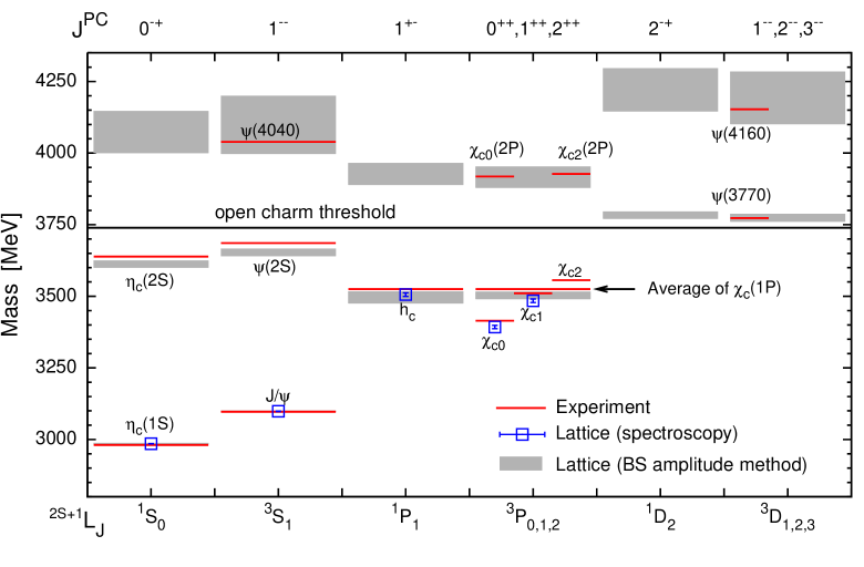
Figure 4: Mass spectrum of charmonium states below and near the open-charm threshold. The vertical scale is in units of MeV. Labels of ${}^{2S+1}[L]_{J}$ ($J^{PC}$) are displayed in lower (upper) horizontal axis. Rectangular boxes indicate predictions from the NRp models with theoretical inputs based on lattice QCD and their errors which are the sum of the statistical and systematic added in quadrature. Solid lines indicate experimental values of well established charmonium states, while square symbols represent results of the standard lattice spectroscopy. A horizontal line shows the open-charm threshold. A symbol of ${\overline{{}^{3}P_{J}}}$ denotes the spin-weighted average of spin-triplet ${}^{3}P_{J}$ states as $M_{{\overline{\chi_{cJ}}}}=(M_{\chi_{c1}}+3M_{\chi_{c2}}+5M_{\chi_{c2}})/9$.

Table 6: Charmonium mass spectrum is summarized in units of MeV. The labels of AVE and HYP in a column of “state” for $S$-states denotes the spin-averaged mass $(M_{{}^{1}S_{0}}+3M_{{}^{3}S_{1}})/4$ and hyperfine splitting mass $M_{{}^{1}S_{0}}-M_{{}^{3}S_{1}}$. Experimental data (denoted as Exp.) are taken from Particle Data Group, rounded to $1$ MeV Beringer et al. (2012). There are two lattice QCD results. First one is given by the usual spectroscopy, and second one is a result calculated by solving the Schrödinger equation with the charmonium potentials determined from lattice QCD. For the second, first error is statistical, and second error is systematic error due to rotational symmetry breaking. For spin triplet states ${}^{3}[L]_{J}$, the spin-weighted average (${\overline{{}^{3}[L]_{J}}}$) are also included.

state	Exp.	Lattice QCD		NRp model
		spectroscopy	BS amplitude
$\eta_{c}$ $(1^{1}S_{0})$	2981	2985(1)	2985(2)(1)	2982
$J/\psi$ $(1^{3}S_{1})$	3097	3099(1)	3099(2)(1)	3090
AVE	3068	3070(9)	3070(2)(1)	3063
HYP	116	114(1)	113(1)(0)	108
$\eta_{c}$ $(2^{1}S_{0})$	3639		3612(9)(7)	3630
$\psi$ $(2^{3}S_{1})$	3686		3653(12)(5)	3672
AVE	3674		3643(11)(5)	3662
HYP	47		41(6)(3)	42
$\eta_{c}$ $(3^{1}S_{0})$			4074(20)(70)	4043
$\psi$ $(3^{3}S_{1})$	4039		4099(24)(98)	4072
AVE			4092(22)(91)	4065
HYP			25(15)(28)	29
$h_{c}$ $(1^{1}P_{1})$	3525	3506(6)	3496(7)(19)	3516
${\overline{\chi_{cJ}}}$ $({\overline{1^{3}P_{J}}})$	3525		3503(7)(10)	3524
$\chi_{c0}$ $(1^{3}P_{0})$	3415	3393(6)		3424
$\chi_{c1}$ $(1^{3}P_{1})$	3511	3485(6)		3505
$\chi_{c2}$ $(1^{3}P_{2})$	3556			3556
$h_{c}$ $(2^{1}P_{1})$			3927(16)(34)	3934
${\overline{\chi_{cJ}}}$ $({\overline{2^{3}P_{J}}})$			3916(19)(31)	3943
$\chi_{c0}$ $(2^{3}P_{0})$	3918			3852
$\chi_{c1}$ $(2^{3}P_{1})$				3925
$\chi_{c2}$ $(2^{3}P_{2})$	3927			3972
$\eta_{c2}$ $(1^{1}D_{2})$			3783(12)(4)	3799
${\overline{\psi}}$ $({\overline{1^{3}D_{J}}})$			3774(13)(2)	3800
$\psi$ $(1^{3}D_{1})$	3773			3785
$\psi$ $(1^{3}D_{2})$				3800
$\psi$ $(1^{3}D_{3})$				3806
$\eta_{c2}$ $(2^{1}D_{2})$			4221(21)(72)	4158
${\overline{\psi}}$ $({\overline{2^{3}D_{J}}})$			4193(25)(88)	4159
$\psi$ $(2^{3}D_{1})$	4153			4142
$\psi$ $(2^{3}D_{2})$				4158
$\psi$ $(2^{3}D_{3})$				4167

Fig. 4 shows the mass spectrum of the charmonia below 4200 MeV. Theoretical spectrum plotted as rectangular boxes are given by solving the discrete nonrelativistic Schrödinger equations with theoretical inputs. Quoted errors of charmonium masses are statistical and systematic uncertainties combined in quadrature. For purpose of comparison, both experimental values and results of the standard lattice spectroscopy are plotted together. The experimental values are taken from Particle Data Group Beringer et al. (2012). At first glance, we find that theoretical calculations from the NRp model with lattice inputs are in fairly good agreement with not only the lattice spectroscopy, but also experiments below open charm threshold. All results are also summarized in Table 6. In this study, we succeed in extracting only the spin-spin potential among spin-dependent interquark potentials. Thus at this stage we cannot predict the spin-orbit splitting which is led by the tensor and spin-orbit forces. In other wards, we can compute only the spin-averaged mass for excited states with higher angular momentum such as $\chi_{cJ}$ state.

Our theoretical calculations for charmonium states below the open-charm threshold are in fairly good agreement with the experimental measurements. The point we wish to emphasize here is that our novel approach has no free parameters in solving the Schrödinger equation opposed to the phenomenological NRp model. All of the parameters appeared in the NRp model calculation are solely determined by lattice QCD simulations, where three light hadron masses ($M_{\pi}$, $M_{K}$ and $M_{\Omega}$) are used for inputs to fix the lattice spacing and light quark hopping parameters. Only experimental values of $\eta_{c}$ and $J/\psi$ masses in the charm sector are used to determine the charm quark parameters in the RHQ action. In this sense the new approach proposed here is distinctly different from the existing calculations with the phenomenological quark potential models.

6 Summary

We have calculated the interquark potentials between charm quark and anti-charm quark almost on the physical point. The interquark potential at finite quark mass is defined through the equal-time Bethe-Salpeter wave function. Our simulations have been performed in the vicinity of the physical light quark masses, which corresponds to $M_{\pi}=156$ MeV, using the PACS-CS gauge configurations generated with the Iwasaki gauge action and 2+1 flavors of Wilson clover quark. We use the relativistic charm quark tuned to reproduce the experimental values of $J/\psi$ and $\eta_{c}$ masses. The resulting spin-independent potential shows behavior of Coulomb plus linear form, and their parameters are close to values used in the traditional quark potential models. Also the string breaking due to existence of sea quarks is not observed. On the other hand, the spin-spin potential obtained from the dynamical simulations exhibits the short-range repulsive interaction. Its shape is quite different from the a repulsive $\delta$-function potential induced by the one-gluon exchange which are usually adopted in the quark potential model.

We have calculated the charmonium spectrum by solving nonrelativistic Schrödinger equation with the theoretical input of the spin-independent and spin-spin potentials and the quark kinetic mass. We simply solved the Schrödinger equation with Dirichlet boundary condition in a matrix manner. This approach enable us to directly use the raw data of the charmonium potential without introducing a phenomenological parameterization for the discretized potential data. We found an excellent agreement of low-lying charmonium masses between our results and the experimental data. We emphasize that our novel approach has no free parameters in solving the Schrödinger type equation opposed to conventional phenomenological quark potential models. As for inputs of lattice QCD, we essentially use three light hadron masses ($M_{\pi}$, $M_{K}$ and $M_{\Omega}$) for fixing the lattice spacing and light quark hopping parameters, and two charmonium masses ($M_{\eta_{c}}$ and $M_{J/\psi}$) for determining the parameters of RHQ action.

In order to precisely predict the mass spectrum above the open charm threshold, we must take into account the effects of not only the mass shift caused by mixing the $Q\overline{Q}$ states with $D\bar{D}$ continuum, but also $S$-$D$ mixing due to existence of the tensor force. However, in this work, we simply ignore these effects and also apply our new approach to the charmonium states above the open-charm threshold. The theoretical prediction of the nonrelativistic potential model with lattice inputs is basically consistent with the existing experimental data, although the systematic uncertainties due to the rotational symmetry breaking are rather large. For more comprehensive prediction including spin-orbit splittings, however, we must calculate all spin-dependent terms (spin-spin, tensor and spin-orbit forces). Especially the tensor force introducing the $S$-$D$ mixing would shift even the masses of $1S$-states. Also the larger spatial extent is required to address the systematic uncertainties due to the finite size effect for the higher excited state that are supposed to possess wider wavefunction.

References

- Eichten et al. (1975) E. Eichten, K. Gottfried, T. Kinoshita, J. B. Kogut, K. Lane, et al., Phys.Rev.Lett. 34, 369–372 (1975).
- Godfrey and Isgur (1985) S. Godfrey, and N. Isgur, Phys.Rev. D32, 189–231 (1985).
- Barnes et al. (2005) T. Barnes, S. Godfrey, and E. Swanson, Phys.Rev. D72, 054026 (2005), hep-ph/0505002.
- Eichten and Feinberg (1981) E. Eichten, and F. Feinberg, Phys.Rev. D23, 2724 (1981).
- Koma and Koma (2007) Y. Koma, and M. Koma, Nucl.Phys. B769, 79–107 (2007), %****␣template-8s.bbl␣Line␣25␣****hep-lat/0609078.
- Koma and Koma (2010) Y. Koma, and M. Koma, Prog.Theor.Phys.Suppl. 186, 205–210 (2010).
- Bali (2001) G. S. Bali, Phys.Rept. 343, 1–136 (2001), hep-ph/0001312.
- Bali et al. (1997a) G. S. Bali, K. Schilling, and A. Wachter, Phys.Rev. D55, 5309–5324 (1997a), hep-lat/9611025.
- Bali et al. (1997b) G. S. Bali, K. Schilling, and A. Wachter, Phys.Rev. D56, 2566–2589 (1997b), hep-lat/9703019.
- Kawanai and Sasaki (2014) T. Kawanai, and S. Sasaki, Phys.Rev. D89, 054507 (2014), 1311.1253.
- Kawanai and Sasaki (2011) T. Kawanai, and S. Sasaki, Phys.Rev.Lett. 107, 091601 (2011), hep-lat/1102.3246.
- Kawanai and Sasaki (2012) T. Kawanai, and S. Sasaki, Phys.Rev. D85, 091503 (2012), 1110.0888.
- Aoki et al. (2009) S. Aoki, et al., Phys.Rev. D79, 034503 (2009), 0807.1661.
- Aoki et al. (2003) S. Aoki, Y. Kuramashi, and S.-i. Tominaga, Prog.Theor.Phys. 109, 383–413 (2003), hep-lat/0107009.
- Ishii et al. (2007) N. Ishii, S. Aoki, and T. Hatsuda, Phys.Rev.Lett. 99, 022001 (2007), nucl-th/0611096.
- Aoki et al. (2010) S. Aoki, T. Hatsuda, and N. Ishii, Prog.Theor.Phys. 123, 89–128 (2010), 0909.5585.
- Velikson and Weingarten (1985) B. Velikson, and D. Weingarten, Nucl.Phys. B249, 433 (1985).
- Gupta et al. (1993) R. Gupta, D. Daniel, and J. Grandy, Phys.Rev. D48, 3330–3339 (1993), hep-lat/9304009.
- Luscher (1991) M. Luscher, Nucl.Phys. B354, 531–578 (1991).
- Caswell and Lepage (1978) W. E. Caswell, and G. P. Lepage, Phys.Rev. A18, 810 (1978).
- Ikeda and Iida (2012) Y. Ikeda, and H. Iida, Prog.Theor.Phys. 128, 941–954 (2012), 1102.2097.
- Aoki et al. (2006) S. Aoki, et al., Phys.Rev. D73, 034501 (2006), hep-lat/0508031.
- Iwasaki (1983) Y. Iwasaki (1983), 1111.7054.
- Kayaba et al. (2007) Y. Kayaba, et al., JHEP 0702, 019 (2007), hep-lat/0611033.
- El-Khadra et al. (1997) A. X. El-Khadra, A. S. Kronfeld, and P. B. Mackenzie, Phys.Rev. D55, 3933–3957 (1997), hep-lat/9604004.
- Christ et al. (2007) N. H. Christ, M. Li, and H.-W. Lin, Phys.Rev. D76, 074505 (2007), hep-lat/0608006.
- Namekawa et al. (2011) Y. Namekawa, et al., Phys.Rev. D84, 074505 (2011), 1104.4600.
- Beringer et al. (2012) J. Beringer, et al., Phys.Rev. D86, 010001 (2012).
- McNeile and Michael (2004) C. McNeile, and C. Michael, Phys.Rev. D70, 034506 (2004), hep-lat/0402012.
- de Forcrand et al. (2004) P. de Forcrand, et al., JHEP 0408, 004 (2004), hep-lat/0404016.
- Levkova and DeTar (2011) L. Levkova, and C. DeTar, Phys.Rev. D83, 074504 (2011), 1012.1837.
- Laschka et al. (2012) A. Laschka, N. Kaiser, and W. Weise, Phys.Lett. B715, 190–193 (2012), 1205.3390.
- Koma et al. (2006) Y. Koma, M. Koma, and H. Wittig, Phys.Rev.Lett. 97, 122003 (2006), hep-lat/0607009.
- Koma and Koma (2009) Y. Koma, and M. Koma, PoS LAT2009, 122 (2009), 0911.3204.
- Charron (2014) B. Charron, PoS LATTICE2013, 223 (2014), 1312.1032.