Probabilities of concurrent extremes

Abstract

The statistical modelling of spatial extremes has recently made major advances. Much of its focus so far has been on the modelling of the magnitudes of extreme events but little attention has been paid on the timing of extremes. To address this gap, this paper introduces the notion of extremal concurrence. Suppose that one measures precipitation at several synoptic stations over multiple days. We say that extremes are concurrent if the maximum precipitation over time at each station is achieved simultaneously, e.g., on a single day. Under general conditions, we show that the finite sample concurrence probability converges to an asymptotic quantity, deemed extremal concurrence probability. Using Palm calculus, we establish general expressions for the extremal concurrence probability through the max-stable process emerging in the limit of the componentwise maxima of the sample. Explicit forms of the extremal concurrence probabilities are obtained for various max-stable models and several estimators are introduced. In particular, we prove that the pairwise extremal concurrence probability for max-stable vectors is precisely equal to the Kendall’s $\tau$. The estimators are evaluated by using simulations and applied to study the concurrence patterns of temperature extremes in the United States. The results demonstrate that concurrence probability can provide a powerful new perspective and tools for the analysis of the spatial structure and impact of extremes.

Keywords: Max-stable process, Poisson point process, Slyvniak formula, Concurrence, Kendall’s $\tau$, Temperature.

1 Introduction

While most of the time extreme value analysis focuses on the magnitude of extreme events, i.e., how large extremes events are, little interest has been paid to their genesis. This paper tries to fill in this gap by looking at what we shall call concurrency of extremes, e.g., have two locations been impacted by the same extreme event or was it a consequence of two different ones? For example, one could observe daily rainfall at various weather stations and would like to quantify the risk that the rainfall extremes over a spatial domain are due to a single extreme event, i.e., a large storm, affecting the entire area. Although potentially rare, such events have great socio-economic consequences and their probabilities should be assessed precisely.

More formally, given a sequence $X_{1},\ldots,X_{n}$ of independent copies of a stochastic process $X$ defined on a compact set $\mathcal{X}\subset\mathbb{R}^{d}$, $d\geq 1$, we say that extremes are sample concurrent at locations $s_{1},\ldots,s_{k}\in\mathcal{X}$, $k\geq 2$, if

$$\max_{i=1,\ldots,n}X_{i}(s_{j})=X_{\ell}(s_{j}),\qquad j=1,\ldots,k,$$ (1)

for some $\ell\in\{1,\ldots,n\}$. Clearly this means that only the observation $X_{\ell}$ contributes to the pointwise maxima at locations $s_{1},\ldots,s_{k}$. It occurs with probability

$$p_{n}(s_{1},\ldots,s_{k})=\mathbb{P}\left[\text{for some $\ell\in\{1,\ldots,n\}\colon\max_{i=1,\ldots,n}X_{i}(s_{j})=X_{\ell}(s_{j})$, $j=1,\ldots,k$}\right],$$ (2)

henceforth referred to as sample concurrence probability.

Provided that $X$ has continuous margins it is not difficult to see that

$$p_{n}(s_{1},\ldots,s_{k})=n\mathbb{E}\left[F\left\{X(s_{1}),\ldots,X(s_{k})\right\}^{n-1}\right],$$

where $F$ is the multivariate cumulative distribution of $\{X(s_{1}),\ldots,X(s_{k})\}$. Interestingly, concurrence of extremes event is invariant under increasing transformations of the marginals so that the concurrence probability does not depend on the marginal distributions of $X$ but only on its dependence structure, i.e., the copula $C$ associated to $F$.

One drawback of the sample concurrence probability $p_{n}(s_{1},\ldots,s_{k})$ is that it varies with the number of observations $n$. Surprisingly, however, we prove in Theorem 1 below that, under mild regularity conditions, this quantity stabilizes to a universal large sample limit

$$p_{n}(s_{1},\ldots,s_{k})\longrightarrow p(s_{1},\ldots,s_{k}),\qquad n\to\infty.$$ (3)

Throughout this paper, we will call the limiting probability $p(s_{1},\ldots,s_{k})$ the extremal concurrence probability. This asymptotic quantity is naturally expressed in terms of a max-stable process $\eta$ emerging in the limit of the normalized maxima in (1), as $n\to\infty$. A direct, intuitive, and equivalent definition of the extremal concurrence probability can be given in terms of the spectral representation of this max-stable process $\eta$.

Following de Haan, [1984], Penrose, [1992] and Schlather, [2002], let

$$\eta(s)=\max_{i\geq 1}\zeta_{i}Y_{i}(s)\qquad s\in\mathcal{X},$$ (4)

where $\{\zeta_{i}\colon i\geq 1\}$ are the points of a Poisson process on $(0,\infty)$ with intensity measure $\zeta^{-2}\mbox{d$\zeta$}$, $Y_{i}$ are independent copies of a non negative stochastic process with continuous sample paths such that $\mathbb{E}\{Y(s)\}=1$ for all $s\in\mathcal{X}$ and $\mathbb{E}\{\sup_{s\in\mathcal{X}}Y(s)\}<\infty$. It is often more convenient to rewrite (4) into

$$\eta(s)=\max_{\varphi\in\Phi}\varphi(s),\qquad s\in\mathcal{X},$$ (5)

where $\Phi=\{\varphi_{i}\colon i\geq 1\}$ with $\varphi_{i}=\zeta_{i}Y_{i}$ is a Poisson point process on $\mathbb{C}_{0}$, the space of non negative continuous functions on $\mathcal{X}$. Within this framework, we now say that extremes are concurrent at $s_{1},\ldots,s_{k}\in\mathcal{X}$ if

$$\eta(s_{j})=\varphi_{\ell}(s_{j}),\qquad j=1,\ldots,k,$$ (6)

for some $\ell\geq 1$, and similarly to the definition of the sample concurrence probability (2), the extremal concurrence probability is defined by

$$p(s_{1},\ldots,s_{k})=\mathbb{P}\left\{\text{for some $\ell\geq 1\colon\eta(s_{j})=\varphi_{\ell}(s_{j})$, $j=1,\ldots,k$}\right\}.$$ (7)

When $k=2$ the extremal concurrence probability $p(s_{1},s_{2})$ coincides with the dependence measure considered in Weintraub, [1991] to study mixing properties of max-stable processes. Another well known measure of dependence is the pairwise extremal coefficient [Schlather and Tawn,, 2003; Cooley et al.,, 2006]

$$\theta(s_{1},s_{2})=-\log\mathbb{P}\{\eta(s_{1})\leq 1,\eta(s_{2})\leq 1\},\qquad s_{1},s_{2}\in\mathcal{X}.$$ (8)

Interestingly, the extremal concurrence probability and the pairwise extremal coefficient share connections. For instance Proposition 5.1 in Stoev, [2008] implies

$$\frac{1}{2}\{2-\theta(s_{1},s_{2})\}\leq p(s_{1},s_{2})\leq 2\{2-\theta(s_{1},s_{2})\},$$ (9)

and we shall see later that the properties of the extremal concurrence probability are similar to that of the pairwise extremal coefficient.

The structure of the paper is as follows. In Section 2 we make connections between sample concurrence probabilities and their extremal counterparts and derive their properties. Section 3 gives closed forms for various parametric max-stable models, and Section 4 introduces various estimators for the sample/extremal concurrence probabilities. The proposed estimators are then analyzed in a simulation study in Section 5 and applied to US continental temperature extremes in Section 6.

2 Concurrence of extremes

In this section we show that sample concurrence probabilities converge to extremal concurrence ones under rather mild domain of attraction conditions. We then provide formulas for the extremal concurrence probability based on the spectral representation of the associated max-stable process and establish their basic properties.

2.1 Sample and extremal concurrence

Concurrence of extremes can be defined through the more general notion of a hitting scenario, which reflects precisely how many different events contribute to the componentwise maximum. Let $X_{1},\ldots,X_{n}$ be a sequence of independent copies of a stochastic process $X$ defined on $\mathcal{X}$ and $s_{1},\ldots,s_{k}\in\mathcal{X}$ be different locations. We suppose that $X$ has continuous marginals to ensure that $\{X_{1}(s_{j}),\ldots,X_{n}(s_{j})\}$ has no ties almost surely and that the maximum is uniquely reached. Let $M_{n}(s)=\max_{i=1,\ldots,n}X_{i}(s)$ be the componentwise maximum and consider the sets $C_{i}=\{j\colon M_{n}(s_{j})=X_{i}(s_{j})\}$, $i=1,\ldots,n$, that account for the location where the $i$-th component $X_{i}$ dominates the rest. Some of these sets may be empty, but from the above discussion, with probability one the non-empty ones are disjoint and form a random partition of $\{1,\ldots,k\}$. This partition $\pi_{n}=\{C_{i}\colon C_{i}\neq\emptyset\}$ will be referred to as the sample hitting scenario.

By analogy with extremal concurrence, one can define an extremal hitting scenario associated to a max-stable process by using the underlying Poisson point process [Wang and Stoev,, 2011; Dombry et al.,, 2013; Dombry and Éyi-Minko,, 2013]. More precisely, for $\eta$ as in (5), the extremal hitting scenario $\pi$ is defined as the random partition of $\{1,\ldots,k\}$ such that two indices $j_{1},j_{2}\in\{1,\ldots,k\}$ are in the same component of $\pi$ if and only if

$$\underset{i\geq 1}{\arg\max}\ \varphi_{i}(s_{j_{1}})=\underset{i\geq 1}{\arg\max}\ \varphi_{i}(s_{j_{2}}).$$

Whatever type of concurrence is considered, i.e., sample concurrence (1) or extremal concurrence (6), extremes are said concurrent if and only if $\pi_{n}=\{1,\ldots,k\}$ or $\pi=\{1,\ldots,k\}$. The next theorem shows the convergence of the sample hitting scenario to the extremal one.

Theorem 1.

Assume that $[h_{1}\{X(s_{1})\},\ldots,h_{k}\{X(s_{k})\}]$ belongs to the maximum domain of attraction of $\{\eta(s_{1}),\ldots,\eta(s_{k})\}$, for some strictly increasing deterministic functions $h_{i}$, $i=1,\ldots,k$. Then, the sample hitting scenario $\pi_{n}$ converges weakly as $n\to\infty$ to the extremal hitting scenario $\pi$ associated to the max-stable process $\eta$.

Proof.

Let $X_{1},X_{2},\ldots$ be a sequence of independent copies of $X$ observed at some locations $s=(s_{1},\ldots,s_{k})\in\mathcal{X}^{k}$, $k\geq 2$. For brevity we will use componentwise algebra (sum, maximum, etc.) and write $X(s)=\{X(s_{1}),\ldots,X(s_{k})\}$. Since the hitting scenario is invariant to strictly increasing deterministic transformations of the marginals, we can assume without loss of generality that $h_{i}(x)=x$, $i=1,\ldots,k$. By assumptions the componentwise maxima $M_{n}(s)=\{\max_{i=1,\ldots,n}X_{i}(s_{1}),\ldots,\max_{i=1,\ldots,n}X_{i}(s_{k})\}$ converge in distribution

$$\frac{M_{n}(s)-b_{n}(s)}{a_{n}(s)}\longrightarrow\eta(s),\qquad n\to\infty,$$

where $a_{n}(s)>0$ and $b_{n}(s)\in\mathbb{R}$. It is well known that the above convergence is equivalent to the convergence of the point process

$$\Phi_{n}=\left\{\frac{X_{i}(s)-b_{n}(s)}{a_{n}(s)}\colon i=1,\ldots,n\right\}\subset\mathbb{R}^{k}.$$

to a Poisson point process $\Phi$ on ${[0,\infty)}^{k}\setminus\{0\}$ where the convergence is meant in the space of point measures $\mathscr{M}_{p}({[0,\infty]}^{k}\setminus\{0\})$ equipped with the metric of vague convergence [Resnick,, 1987].

Consider the mapping

$$\Pi\colon\mathscr{M}_{p}({[0,\infty]}^{k}\setminus\{0\}) \longrightarrow\mathscr{P}_{k}$$

$$\Psi \longmapsto\Pi(\Psi),$$

where $\mathscr{P}_{k}$ is the set of all possible partitions of $\{1,\ldots,k\}$ and $\Pi(\Psi)$ is the hitting scenario associated to the collection of functions $\Psi=\{\psi_{i}\colon i\in I\}$, $I\subseteq\mathbb{N}$. Clearly, $\pi_{n}=\Pi(\Phi_{n})$ and $\pi=\Pi(\Phi)$. Since the map $\Pi$ is well defined and continuous at each point $\Psi\in\mathscr{M}_{p}({[0,\infty]}^{k}\setminus\{0\})$ for which the maxima are uniquely defined, see Appendix A.1, we can apply the continuous mapping theorem to show that the weak convergence $\Phi_{n}\to\Phi$ entails the weak convergence $\pi_{n}\to\pi$. ∎

Remark.

A direct consequence of Theorem 1 is that, provided the stochastic process $X$ is in the domain of attraction of some max-stable process $\eta$, the sample concurrence probability converges to its extremal counterpart, i.e.,

$$p_{n}(s_{1},\ldots,s_{k})=\mathbb{P}\left[\pi_{n}=\{1,\ldots,k\}\right]\longrightarrow\mathbb{P}\left[\pi=\{1,\ldots,k\}\right]=p(s_{1},\ldots,s_{k}),\qquad n\to\infty,$$

and proves (3).

2.2 General formulas and properties of extremal concurrence probabilities

The following theorem gives an expression for the extremal concurrence probability $p(s_{1},\ldots,s_{k})$.

Theorem 2.

We have

$$p(s_{1},\ldots,s_{k})=\mathbb{E}_{Y}\left(\left[\mathbb{E}_{\tilde{Y}}\left\{\max_{j=1,\ldots,k}\frac{\tilde{Y}(s_{j})}{Y(s_{j})}\right\}\right]^{-1}\right),$$ (10)

where $Y$ and $\tilde{Y}$ are independent copies of the stochastic process appearing in (4).

Proof.

Let $\Lambda$ denotes the intensity mesaure of the $\mathbb{C}_{0}$-valued Poisson point process $\Phi$ in (5) given by

$$\Lambda(A)=\int_{0}^{\infty}\mathbb{P}(\zeta Y\in A)\zeta^{-2}\mbox{d$\zeta$},$$

for all Borel set $A\subset\mathbb{C}_{0}$. We have

$$p(s_{1},\ldots,s_{k}) =\mathbb{P}\left\{\exists\varphi\in\Phi\colon\varphi(s_{1})=\eta(s_{1}),\ldots,\varphi(s_{k})=\eta(s_{k})\right\}$$

$$=\int_{\mathbb{C}_{0}}\mathbb{P}\left\{f(s_{j})>\tilde{\eta}(s_{j}),j=1,\ldots,k\right\}\Lambda(\mbox{d$f$})$$ (11)

$$=\mathbb{E}_{Y}\left[\int_{0}^{\infty}\mathbb{P}\left\{\tilde{\eta}(s_{j})<\zeta Y(s_{j}),j=1,\ldots,k\right\}\zeta^{-2}\mbox{d$\zeta$}\right]$$

$$=\mathbb{E}_{Y}\left(\int_{0}^{\infty}\exp\left[-\mathbb{E}_{\tilde{Y}}\left\{\max_{j=1,\ldots,k}\frac{\tilde{Y}(s_{j})}{\zeta Y(s_{j})}\right\}\right]\zeta^{-2}\mbox{d$\zeta$}\right)$$

$$=\mathbb{E}_{Y}\left(\left[\mathbb{E}_{\tilde{Y}}\left\{\max_{j=1,\ldots,k}\frac{\tilde{Y}(s_{j})}{Y(s_{j})}\right\}\right]^{-1}\right)$$

where $\tilde{\eta}$ and $\tilde{Y}$ are independent copies of $\eta$ and $Y$ respectively. Note that the second equality uses Slyvniak’s formula, the fourth one the cumulative distribution of the max-stable process $\tilde{\eta}$ and the last one the expectation of an inverse exponential random variable. ∎

Remark.

By the seminal paper of de Haan, [1984] (see also Stoev and Taqqu, [2005]; Kabluchko, [2009]), any continuous in probability max-stable process can be represented as

$$\{\eta(s)\colon s\in\mathcal{X}\}\stackrel{{\scriptstyle\rm d}}{{=}}\left\{\max_{i\geq 1}\zeta_{i}f_{s}(u_{i})\colon s\in\mathcal{X}\right\},$$ (12)

where $\{f_{s}\colon s\in\mathcal{X}\}$ is a collection of non-negative integrable functions on the space $(U,\mathcal{U},\nu)$. Here $\{(\zeta_{i},u_{i})\colon i\geq 1\}$ is a Poisson point process on $(0,\infty)\times U$ with intensity $\zeta^{-2}\mbox{d$\zeta$}\nu(\mbox{d$u$})$.

The functions $\{f_{s}\colon s\in\mathcal{X}\}$ are known as spectral functions of $\eta$ and (12) as de Haan’s spectral representation. When $\nu$ is a probability measure, one can view $Y(s)=f_{s}$ as random variables on the probability space $(U,{\cal U},\nu)$ and then (12) becomes (4). Conversely, any representation (12) can be cast in the form (4) with a change of variables. Depending on the context one representation may be more convenient than the other. In terms of (12), the concurrence probability formula in (10) becomes

$$p(s_{1},\ldots,s_{k})=\int_{U}\left[\int_{U}\left\{\max_{j=1,\ldots,k}\frac{f_{s_{j}}(\tilde{u})}{f_{s_{j}}(u)}\right\}\nu(\mbox{d$\tilde{u}$})\right]^{-1}\nu(\mbox{d$u$}),$$ (13)

and the proof is essentially the same.

One could expect from Definition 6 and Theorem 2 that the extremal concurrence probability depends on the distribution of the spectral process $Y$ in (4) or the choice of spectral functions in (12). These representations are not unique, but we will see in the theorem below that the extremal concurrence probability $p(s_{1},\ldots,s_{k})$ depends only on the distribution of the max-stable process $\eta$ and not on the choice of the specific spectral representation.

Theorem 3.

For $s_{1},\ldots,s_{k}\in\mathcal{X}$, $k\geq 2$, we have

$$p(s_{1},\ldots,s_{k})=\sum_{r=1}^{k}(-1)^{r}\sum_{\begin{smallmatrix}J\subseteq\{1,\ldots,k\}\\ |J|=r\end{smallmatrix}}\mathbb{E}_{\tilde{\eta}}\left[\log\mathbb{P}_{\eta}\left\{\eta(s_{j})\leq\tilde{\eta}(s_{j}),j\in J\right\}\right],$$ (14)

where $\tilde{\eta}$ is an independent copy of $\eta$. In particular when $k=2$,

$$p(s_{1},s_{2})=2+\mathbb{E}_{\tilde{\eta}}\left[\log\mathbb{P}_{\eta}\left\{\eta(s_{j})\leq\tilde{\eta}(s_{j}),j=1,2\right\}\right].$$ (15)

Proof.

Starting from (11) and applying the inclusion-exclusion formula, we have

$$p(s_{1},\ldots,s_{k}) =\mathbb{E}_{\tilde{\eta}}\left[\Lambda\left(\left\{\text{$f(s_{j})>\tilde{\eta}(s_{j})$ for some $j\in\{1,\ldots,k\}$}\right\}\right)\right]$$

$$=\mathbb{E}_{\tilde{\eta}}\left[\sum_{r=1}^{k}\sum_{\begin{smallmatrix}J\subseteq\{1,\ldots,k\}\\ |J|=r\end{smallmatrix}}(-1)^{r+1}\Lambda\left(\left\{f(s_{j})>\tilde{\eta}(s_{j}),j\in J\right\}\right)\right].$$

Since the cumulative distribution function of $\eta$ is $\mathbb{P}_{\eta}\left\{\eta(s_{j})\leq\tilde{\eta}(s_{j}),j\in J\right\}=\exp\left[-\Lambda\left(\left\{f(s_{j})>\tilde{\eta}(s_{j}),j\in J\right\}\right)\right]$, we get

$$p(s_{1},\ldots,s_{k})=\sum_{r=1}^{k}(-1)^{r}\sum_{\begin{smallmatrix}J\subseteq\{1,\ldots,k\}\\ |J|=r\end{smallmatrix}}\mathbb{E}_{\tilde{\eta}}\left[\log\mathbb{P}_{\eta}\left\{\eta(s_{j})\leq\tilde{\eta}(s_{j}),j\in J\right\}\right].$$

The simplification when $k=2$ is straightforward because when $|J|=1$ we have

$$\mathbb{E}_{\tilde{\eta}}\left[\log\mathbb{P}_{\eta}\left\{\eta(s_{j})\leq\tilde{\eta}(s_{j}),j\in J\right\}\right]=\mathbb{E}_{\tilde{\eta}}\left\{-\tilde{\eta}(s_{j})^{-1}\right\}=-1,$$

as $\tilde{\eta}(s_{j})^{-1}$ is a standard exponential random variable. ∎

In the remaining part of this section, we investigate some properties of the extremal concurrence probabilities. Surprisingly, although the two notions are different, we encounter strong similarities with the extremal coefficient (8). We recall that the extremal coefficient $\theta(s_{1},s_{2})$ takes values in $[1,2]$, the lower and upper bounds correspond to perfect dependence and independence respectively. The next proposition states a similar result for the extremal concurrence probability.

Proposition 1.

For all $s_{1},s_{2}\in\mathcal{X}$, we have

• $p(s_{1},s_{2})=0$ if and only if $\eta(s_{1})$ and $\eta(s_{2})$ are independent;

• $p(s_{1},s_{2})=1$ if and only if $\eta(s_{1})$ and $\eta(s_{2})$ are almost surely equal.

The proof uses the following generalization and improvement of the upper bound in (9).

Lemma 1.

For all $s_{1},\ldots,s_{k}\in\mathcal{X}$, $k\geq 2$, we have $p(s_{1},\ldots,s_{k})\leq\mathbb{E}\left\{\min_{j=1,\ldots,k}Y(s_{j})\right\}$.

Proof.

In the context of Theorem 2, we have (by conditioning on $Y$)

$$\mathbb{E}_{\tilde{Y}}\left\{\max_{j=1,\ldots,k}\frac{\tilde{Y}(s_{j})}{Y(s_{j})}\right\}\geq\max_{j=1,\ldots,k}Y(s_{j})^{-1}\mathbb{E}_{\tilde{Y}}\left\{\tilde{Y}(s_{j})\right\}=\left\{\min_{j=1,\ldots,k}Y(s_{i})\right\}^{-1},$$

since $\mathbb{E}_{\tilde{Y}}\{\tilde{Y}(s_{j})\}=1$. This, in view of (10) implies the desired result. ∎

Proof of Proposition 1.

Equation (9) implies that $p(s_{1},s_{2})=0$ if and only if $\theta(s_{1},s_{2})=2$ which is equivalent to the independence of $\eta(s_{1})$ and $\eta(s_{2})$. When $p(s_{1},s_{2})=1$, Lemma 1 entails $Y(s_{1})=Y(s_{2})$ almost surely so that $\eta(s_{1})=\eta(s_{2})$ almost surely. It is easy to prove the converse implication: if $\eta(s_{1})$ and $\eta(s_{2})$ are almost surely equal, the same holds for $Y(s_{1})$ and $Y(s_{2})$ so that $p(s_{1},s_{2})=1$. ∎

Interestingly $p(s_{1},\ldots,s_{k})$ can be expressed via the extremal coefficients of another max-stable process.

Proposition 2.

Let $\eta$ be a simple max-stable process as defined in (4) and $\tilde{\eta},\tilde{\eta}_{1},\tilde{\eta}_{2},\ldots$ independent copies of it. Consider the simple max-stable process

$$\xi(s)=\max_{i\geq 1}\zeta_{i}\frac{Y_{i}(s)}{\tilde{\eta}_{i}(s)},\qquad s\in\mathcal{X},$$

then

$$p(s_{1},\ldots,s_{k})=\sum_{r=1}^{k}(-1)^{r+1}\sum_{\begin{smallmatrix}J\subseteq\{1,\ldots,k\}\\ |J|=r\end{smallmatrix}}\theta_{\xi}(s_{j},j\in J),$$

where $\theta_{\xi}(s_{j},j\in J)=-\log\mathbb{P}\{\xi(s_{j})\leq 1,j\in J\}$. In particular $p(s_{1},s_{2})=2-\theta_{\xi}(s_{1},s_{2})$.

Proof.

Clearly $\xi$ is a simple max-stable process since both $Y$ and $\tilde{\eta}$ are non negative and $\mathbb{E}\{Y(s)/\tilde{\eta}(s)\}=1$ for all $s\in\mathcal{X}$. We have

$$\mathbb{E}_{\tilde{\eta}}\left[\log\mathbb{P}_{\eta}\left\{\eta(s_{j})\leq\tilde{\eta}(s_{j}),j\in J\right\}\right]=-\mathbb{E}_{\tilde{\eta}}\left[\mathbb{E}_{Y}\left\{\max_{j\in J}\frac{Y(s_{j})}{\tilde{\eta}(s_{j})}\right\}\right]=\log\mathbb{P}_{\xi}\left\{\xi(s_{j})\leq 1,j\in J\right\}=-\theta_{\xi}(s_{j},j\in J).$$

∎

The next corollary lists some properties of the extremal concurrence probability function that closely parallel those of the extremal coefficient function. In view of Proposition 2, the proof follows as in Schlather and Tawn, [2003] or Cooley et al., [2006].

Corollary.

Let $p\colon h\mapsto p(o,h)$ be an extremal concurrence probability function associated to a stationary max-stable process in $\mathcal{X}$ for some arbitrary origin $o\in\mathcal{X}$ and $h\in\mathcal{X}$. Then the following assertions hold.

• The function $h\mapsto p(h)$ is positive semidefinite;

• The function $h\mapsto p(h)$ is not differentiable at the origin unless $p(h)=1$ for all $h\in\mathcal{X}$;

• If $d\geq 1$ and if $\eta$ is isotropic, then $h\mapsto p(h)$ has at most a jump at the origin and is continuous elsewhere;

• $\{2-p(h_{1}+h_{2})\}\leq\{2-p(h_{1})\}\{2-p(h_{2})\}$ for all $h_{1},h_{2}\in\mathcal{X}$;

• $\{2-p(h_{1}+h_{2})\}^{\alpha}\leq\{2-p(h_{1})\}^{\alpha}+\{2-p(h_{2})\}^{\alpha}-1$ for all $h_{1},h_{2}\in\mathcal{X}$ and $0\leq\alpha\leq 1$;

• $\{2-p(h_{1}+h_{2})\}^{\alpha}\geq\{2-p(h_{1})\}^{\alpha}+\{2-p(h_{2})\}^{\alpha}-1$ for all $h_{1},h_{2}\in\mathcal{X}$ and $\alpha<0$.

We conclude this section with an unexpected result that relates the bivariate extremal concurrence probability with the well known Kendall’s $\tau$.

Theorem 4.

For any max-stable process $\eta$, we have $p(s_{1},s_{2})=\tau$ where $\tau=\mathbb{E}\left[\mbox{sign}\{\eta(s_{1})-\eta_{*}(s_{1})\}\mbox{sign}\{\eta(s_{2})-\eta_{*}(s_{2})\}\right]$ is the Kendall’s $\tau$ of $\{\eta(s_{1}),\eta(s_{2})\}$ and $\eta_{*}$ is an independent copy of $\eta$.

Proof.

Let $W=F\{\eta(s_{1}),\eta(s_{2})\}$ where $F$ is the bivariate cumulative distribution function of $\{\eta(s_{1}),\eta(s_{2})\}$. From (15) we have $p(s_{1},s_{2})=2+\mathbb{E}\left(\log W\right)$. But since $\{\eta(s_{1}),\eta(s_{2})\}$ is a bivariate max-stable random vector, we know that $\mathbb{P}(W\leq w)=w-(1-\tau)w\log w$, $0\leq w\leq 1$ [Ghoudi et al.,, 1998] and hence, after some simple calculations, $p(s_{1},s_{2})=\tau$. ∎

3 Formulas for extremal concurrence probabilities

In this section we gather formulas for the extremal concurrence probabilities for some popular models of max-stable random vectors and processes. As we will see, it is not always possible to get explicit formulas, and in such situations, we propose to use Monte-Carlo methods.

3.1 Closed forms

Example 1 (Logistic model).

The concurrence probability for the $k$-variate logistic model, i.e., with cumulative distribution

$$F(z_{1},\ldots,z_{k})=\exp\left\{-\left(\sum_{j=1}^{k}z_{j}^{-1/\alpha}\right)^{\alpha}\right\},\qquad 0<\alpha\leq 1,\quad z_{1},\ldots,z_{k}>0,$$

is $p(s_{1},\ldots,s_{k})=\prod_{j=1}^{k-1}(1-\alpha/j)$.

Recall that for this model independence is reached when $\alpha=1$ while perfect dependence occurs as $\alpha\downarrow 0$ and, as expected, for such situations we have $p(s_{1},\ldots,s_{k})=0$ and $p(s_{1},\ldots,s_{k})=1$ respectively.

Proof.

It is not difficult to see that the multivariate logistic model corresponds to the case where $Y$ in (4) is a pure noise process with margins such that $\mathbb{P}\{Y(s)<y\}=\exp[-\{\Gamma(1-\alpha)y\}^{-1/\alpha}]$ where $\Gamma$ is the Gamma function. Using Theorem 2, we have

$$p(s_{1},\ldots,s_{k}) =\mathbb{E}_{Y}\left(\left[\mathbb{E}_{\tilde{Y}}\left\{\max_{j=1,\ldots,k}\frac{\tilde{Y}(s_{j})}{Y(s_{j})}\right\}\right]^{-1}\right)=\mathbb{E}_{Y}\left(\left[-\log F\{\tilde{Y}(s_{1}),\ldots,\tilde{Y}(s_{k})\}\right]^{-1}\right)$$

$$=\mathbb{E}_{Y}\left[\left\{\sum_{j=1}^{k}Y(s_{j})^{-1/\alpha}\right\}^{-\alpha}\right]=\frac{\Gamma(k-\alpha)}{\Gamma(k)\Gamma(1-\alpha)}=\prod_{j=1}^{k-1}(1-\alpha/j),$$

where the fourth equality used the fact that $\sum_{j=1}^{k}Y(s_{j})^{-1/\alpha}$ is a Gamma random variable with scale $\Gamma(1-\alpha)^{1/\alpha}$ and shape $k$ for which negative moments are known. ∎

Example 2 (Max-linear model).

Consider the max-linear model $\eta(s)=\max_{m=1,\ldots,n}\varphi_{m}(s)Z_{m}$, where $Z_{1},\ldots,Z_{n}$ are independent unit Fréchet random variables and some functions $\{s\mapsto\varphi_{m}(s)\in\mathbb{C}_{0},m=1,\ldots,n\}$ such that $\sum_{m=1}^{n}\varphi_{m}(s)=1$ for all $s\in\mathcal{X}$. We have

• The concurrence probability equals

  $$p(s_{1},\ldots,s_{k})=\sum_{\ell=1}^{n}p_{\ell}(s_{1},\ldots,s_{k}),\qquad p_{\ell}(s_{1},\ldots,s_{k})=\left\{\sum_{m=1}^{n}\max_{j=1,\ldots,k}\frac{\varphi_{m}(s_{j})}{\varphi_{\ell}(s_{j})}\right\}^{-1},$$ (16)

  with the convention that $0/0=0$, $a/0=\infty$ if $a>0$, and $1/\infty=0$.

• The probability that component $\ell$ dominates at sites $s_{1},\ldots,s_{k}$ is given by the term $p_{\ell}$ in (16), i.e.,

  $$p_{\ell}(s_{1},\ldots,s_{k})=\mathbb{P}\left\{\eta(s_{j})=\varphi_{\ell}(s_{j})Z_{\ell},\ j=1,\ldots,k\right\}$$ (17)

Proof.

Part i) is an immediate consequence of (13). Indeed, let $U=\{1,\ldots,n\}$ be equipped with the counting measure $\nu\{1\}=\cdots=\nu\{n\}=1$. By taking $f_{s}(m)=\varphi_{m}(s)$, $m\in U$, we obtain that the max-linear model has the representation (12). The integral expression of the concurrence probability in (13) then becomes a sum of the terms $p_{\ell}$ in (16).

Part ii) shows an intriguing fact that the concurrence probability $p(s_{1},\ldots,s_{k})$ for the max-linear model is the sum of the probabilities that one of the $n$ components dominates the rest. Indeed, by the max-stability property and the independence of the unit Fréchet random variables $Z_{m}$’s, we have that the right-hand side of (17) equals

$$\mathbb{P}\left\{\max_{m\neq\ell}\max_{j=1,\ldots,k}\frac{\varphi_{m}(s_{j})}{\varphi_{\ell}(s_{j})}Z_{m}\leq Z_{\ell}\right\}=\mathbb{P}(aZ_{1}\leq Z_{2}),$$

where $a=\sum_{m\neq\ell}\max_{j=1,\ldots,k}{\varphi_{m}(s_{j})/\varphi_{\ell}(s_{j})}$. Equation (17) follows from the fact that $\mathbb{P}(aZ_{1}\leq Z_{2})=(1+a)^{-1}$, $a\geq 0$. ∎

Example 3 (Chentsov random fields).

Suppose that the process $Y(s)=1_{A}(s)$, where $A\subset\mathbb{R}^{d}$ is a random set. Then, by analogy with the theory of symmetric $\alpha$-stable process [Samorodnitsky and Taqqu,, 1994, Chap. 8], the max-stable process

$$\eta(s)=\max_{i\geq 1}\zeta_{i}1_{A_{i}}(s),\qquad s\in\mathcal{X},$$

where $Y_{i}\equiv 1_{A_{i}}$ are independent copies of $Y\equiv 1_{A}$, will be referred to as a Chentsov max-stable random field on $\mathcal{X}$.

For a Chentsov-type max-stable process we have

$$p(s_{1},\ldots,s_{k})=\mathbb{P}\left(\{s_{1},\ldots,s_{k}\}\subset A\mid\{s_{1},\ldots,s_{k}\}\cap A\neq\emptyset\right),$$ (18)

or less formally that the extremal concurrence probability is the conditional probability that the sites $s_{1},\ldots,s_{k}$ are covered by the random set $A$ given that at least one of the sites is covered.

Proof.

The result is an immediate consequence of Theorem 2. Since the outer expectation in (10) can be restricted to the event $\{\min_{j=1,\ldots,k}Y(s_{j})>0\}$, we have

$$p(s_{1},\ldots,s_{k}) =\mathbb{E}_{Y}\left(\left[\mathbb{E}_{\tilde{Y}}\left\{\max_{j=1,\ldots,k}\frac{1_{\tilde{A}}(s_{j})}{1_{A}(s_{j})}\right\}\right]^{-1}1_{\{\min_{j=1,\ldots,k}1_{A}(s_{j})>0\}}\right)$$

$$=\mathbb{E}_{Y}\left(\left[\mathbb{E}_{\tilde{Y}}\left\{\max_{j=1,\ldots,k}1_{\tilde{A}}(s_{j})\right\}\right]^{-1}\min_{j=1,\ldots,k}1_{A}(s_{j})\right)$$ (19)

$$=\frac{\mathbb{E}\left\{\min_{j=1,\ldots,k}1_{A}(s_{j})\right\}}{\mathbb{E}\left\{\max_{j=1,\ldots,k}1_{A}(s_{j})\right\}},$$

where in the second relation we used the fact that $1_{\{\min_{j=1,\ldots,k}1_{A}(s_{j})\}}=\min_{j=1,\ldots,k}1_{A}(s_{j})$ and that the event $\min_{i=1,\ldots,k}1_{A}(s_{i})>0$ is equivalent to $\{1_{A}(s_{1})=1,\ldots,1_{A}(s_{k})=1\}$. This proves (18). ∎

Example 4 (Extremal processes).

The max-stable process $\{\eta(s)\colon s\in[0,1]\}$ is an extremal process if it has stationary and independent max-increments, i.e.,

$$\{\eta(s_{1}),\ldots,\eta(s_{k})\}\stackrel{{\scriptstyle\rm d}}{{=}}\left[s_{1}Z_{1},\max\{s_{1}Z_{1},(s_{2}-s_{1})Z_{2}\},\ldots,\max\{s_{1}Z_{1},\ldots,(s_{k}-s_{k-1})Z_{k}\}\right],$$

where $0<s_{1}<\cdots<s_{k}$ and $Z_{1},\ldots,Z_{k}$ are independent unit Fréchet random variables. It can be shown that

$$\eta(s)\stackrel{{\scriptstyle\rm d}}{{=}}\max_{i\geq 1}\zeta_{i}1_{[U_{i},1]}(s),\qquad s\in[0,1],$$

where $U_{i}$’s are independent $U(0,1)$ random variables. Using our previous result on Chentsov random fields, we have for all $0<s_{1}<\cdots<s_{k}\leq 1$

$$p(s_{1},\ldots,s_{k})=\frac{\mathbb{P}\left(\{s_{1},\ldots,s_{k}\}\subset[U,1]\right)}{\mathbb{P}\left(\{s_{1},\ldots,s_{k}\}\cap[U,1]\neq\emptyset\right)}=\frac{\mathbb{P}(U\leq s_{1})}{\mathbb{P}(U\leq s_{k})}=\frac{s_{1}}{s_{k}},$$

where $U\sim U(0,1)$. This result is not surprising since for this simple case, extremes are concurrent at locations $0<s_{1}<\cdots<s_{k}<1$ if $\eta(s)$ has no jumps in the interval $[s_{1},s_{k}]$. Hence using the independence and stationarity of the max-increments, the probability of the latter event is $\mathbb{P}\{s_{1}Z_{1}\geq(s_{k}-s_{1})Z_{2}\}=s_{1}/s_{k}$, where $Z_{1}$ and $Z_{2}$ are two independent unit Fréchet variables.

Example 5 (Indicator moving maxima).

In the context of (12), if $f_{s}(u)=1_{A_{s}}(u)$, for some sequence of measurable deterministic sets $A_{s}$, by using (13), we obtain as in (3.1) that

$$p(s_{1},\ldots,s_{k})=\frac{\nu(\cap_{j=1,\ldots,k}A_{s_{j}})}{\nu(\cup_{j=1,\ldots,k}A_{s_{j}})}.$$ (20)

In the simple case $f_{s}(u)=1_{A}(u-s)$, i.e. $A_{s}=s+A$ with some deterministic set $A$, where $\nu$ is the Lebesgue measure on $\mathbb{R}^{d}$, (20) implies

$$p(s,s+h)=p(h)=\frac{|A\cap(h+A)|}{|A\cup(h+A)|}=\frac{c_{A}(h)}{2|A|-c_{A}(h)},$$

where $|A|$ denotes the $d$-dimensional volume of $A$ and $c_{A}(h)=|A\cap(h+A)|$. The latter function and hence the extremal concurrence probability function $p(h)$ can then be obtained in closed form for many different sets. For example, in the case $\eta$ is isotropic, i.e., $A=\{s\in\mathbb{R}^{d}\colon\|x\|\leq r\}$ is the centered ball of radius $r>0$ in Euclidean space, using the formula for the volume of the cap, we obtain

$$c_{A}(\|h\|)=C_{d}r^{d}B_{(d+1)/2,1/2}\left\{\frac{\|h\|(2r-\|h\|)}{2r^{2}}\right\},\qquad C_{d}=\frac{\pi^{d/2}}{\Gamma(1+d/2)},$$

where $B_{a,b}(x)=B(a,b)^{-1}\int_{0}^{x}u^{a-1}(1-u)^{b-1}\mbox{d$u$}$ is the cumulative distribution function of a $\mbox{Beta}(a,b)$ random variable.

3.2 Monte-Carlo methods

It may happen that for some parametric max-stable models, explicit forms for extremal concurrence probabilities are not available but hopefully it is often possible to use Monte-Carlo methods to approximate the theoretical extremal concurrence probabilities with arbitrary precision. A naive strategy would consist in using (10) to devise a Monte-Carlo estimator, but it is wiser to take advantage of the closed forms of max-stable processes cumulative distributions, i.e.,

$$\mathbb{P}\left\{\eta(s_{j})\leq z_{j},j=1,\ldots,k\right\}=\exp\{-V_{s_{1},\ldots,s_{k}}(z_{1},\ldots,z_{k})\},\qquad z_{1},\ldots,z_{k}>0,$$

where $V_{s_{1},\ldots,s_{k}}$ is an homogeneous function of order $-1$. Rewriting (10), we found

$$p(s_{1},\ldots,s_{k}) =\mathbb{E}_{Y}\left(\left[-\log\mathbb{P}_{\tilde{\eta}}\left\{\tilde{\eta}(s_{j})\leq Y(s_{j}),j=1,\ldots,k\right\}\right]^{-1}\right)$$

$$=\mathbb{E}_{Y}\left(\left\{V_{s_{1},\ldots,s_{k}}[Y(s_{1}),\ldots,Y(s_{k})]\right\}^{-1}\right)$$ (21)

which can easily be estimated by sampling independent copies of $Y$ and computing the sample mean. We can often make use of antithetic variables to get more precise estimates. Note that specific choice of the spectral process $Y$ can lead to better strategies as we will illustrate in the following examples.

Example 6 (Brown–Resnick model).

Let $\eta$ be a Brown–Resnick stationary random field on $\mathcal{X}$ driven by a Gaussian process [Kabluchko et al.,, 2009]. That is, the processes $Y_{i}$ in (4) are equal in distribution to

$$Y(s)=\exp\{W(s)-\gamma(s)\},\qquad s\in\mathcal{X},$$ (22)

where $W$ is a zero mean Gaussian random field with stationary increments and semi-variogram $\gamma$, i.e. $2\gamma(h)=\mathbb{E}\{W(h)^{2}\}=\mathbb{E}[\{W(s+h)-W(s)\}^{2}]$, $s,h\in\mathcal{X}$.

For this model, the bivariate extremal concurrence probability function is given by

$$p(o,h)=\mathbb{E}\left(\left[\Phi(Z)+\exp\left\{\gamma(h)-\sqrt{2\gamma(h)}Z\right\}\Phi\left\{\sqrt{2\gamma(h)}-Z\right\}\right]^{-1}\right),$$ (23)

where $Z\sim N(0,1)$ has the standard normal distribution with cumulative distribution function $\Phi$. As expected $p(o)=1$ and $p(h)\to 0$ as $\|h\|\to\infty$ provided that the semi-variogram is unbounded, i.e., $\gamma(h)\to\infty$ as $\|h\|\to\infty$.

Proof.

Without loss of generality, for Brown–Resnick processes we can assume that in (4) we have $Y(o)=1$ almost surely. The bivariate cumulative function is given by $\mathbb{P}\{\eta(0)\leq z_{1},\eta(h)\leq z_{2}\}=\exp\{-V_{h}(z_{1},z_{2})\},\qquad z_{1},z_{2}>0$ with

$$V_{h}(z_{1},z_{2})=\frac{1}{z_{1}}\Phi\left(\sqrt{\gamma(h)/2}+\frac{1}{\sqrt{2\gamma(h)}}\log\frac{z_{2}}{z_{1}}\right)+\frac{1}{z_{2}}\Phi\left(\sqrt{\gamma(h)/2}+\frac{1}{\sqrt{2\gamma(h)}}\log\frac{z_{1}}{z_{2}}\right).$$

Equation (21) together with the fact that $\{Y(o),Y(h)\}$ has the same distribution as $\{1,e^{\sqrt{2\gamma(h)}\,Z-\gamma(h)}\}$ entails

$$p(o,h)=\mathbb{E}\left(\left\{V_{h}[Y(o),Y(h)]\right\}^{-1}\right)=\mathbb{E}\left\{\left(V_{h}\left[1,\exp\left\{\sqrt{2\gamma(h)}\,Z-\gamma(h)\right\}\right]\right)^{-1}\right\}.$$

Equation (23) follows after straightforward simplifications. ∎

A popular special case of the the Brown–Resnick family of models is the moving maximum storm model introduced by Smith, [1990] known also as the Gaussian extremal process. Consider the spectral representation (12), where $U=\mathbb{R}^{d}$ and $\nu$ is the Lebesgue measure. Taking $f_{s}(u)=\varphi_{\Sigma}(s-u)$, where $\varphi_{\Sigma}$ is the multivariate Normal density with zero mean and covariance matrix $\Sigma$, we obtain the max-stable process

$$\eta(s)=\max_{i\geq 1}\zeta_{i}\varphi_{\Sigma}(s-u_{i}),\qquad s\in\mathcal{X}.$$ (24)

Then, the following are true:

• The process $\eta$ belongs to the family of degenerate Brown–Resnick models in (22) with $W(s)=s^{\top}Z$, $s\in{\mathbb{R}}^{d}$ and $Z\sim N(0,\Sigma^{-1})$.

• Consequently, the concurrence probability function of $\eta$ is given by (23) with $\gamma(h)=h^{\top}\Sigma^{-1}h/2$.

Proof.

Let $\eta$ be a Brown–Resnick process with variogram $2\gamma(h)=h^{\top}\Sigma^{-1}h$, that is, we can assume without loss of generality that in the spectral characterization we have $Y(s)=\exp(s^{\top}\Sigma^{-1}Z-s^{\top}\Sigma^{-1}s)$ with $Z\sim N(0,\Sigma)$. Then for all $s_{1},\ldots,s_{k}\in\mathcal{X}$ and $z_{1},\ldots,z_{k}>0$ we have

$$-\log\mathbb{P}\{\eta(s_{j})\leq z_{j},j=1,\ldots,k\} =\mathbb{E}_{Z}\left\{\max_{j=1,\ldots,k}z_{j}^{-1}\exp\left(s_{j}^{\top}\Sigma^{-1}Z-\frac{1}{2}s_{j}^{\top}\Sigma^{-1}s_{j}\right)\right\}$$

$$=(2\pi)^{-k/2}|\Sigma|^{-1/2}\int_{\mathbb{R}^{d}}\max_{j=1,\ldots,k}z_{j}^{-1}\exp\left(-\frac{1}{2}y^{\top}\Sigma^{-1}y+s_{j}^{\top}\Sigma^{-1}y-\frac{1}{2}s_{j}^{\top}\Sigma^{-1}s_{j}\right)\mbox{d$y$}$$

$$=\int_{\mathbb{R}^{d}}\max_{j=1,\ldots,k}z_{j}^{-1}\varphi_{\Sigma}(s_{j}-y)\mbox{d$y$}.$$

The last relation equals the negative log cumulative distribution function of the moving maxima in (24). ∎

Example 7 (Schlather and extremal-$t$ processes).

Let $\eta$ be an extremal-$t$ process on $\mathcal{X}$, i.e., the processes $Y_{i}$ in (4) are equal in distribution to

$$Y(x)=c_{\nu}\max\{0,W(s)\}^{\nu},\quad c_{\nu}=\sqrt{\pi}2^{-(\nu-2)/2}\Gamma\left(\frac{\nu+1}{2}\right)^{-1}\qquad s\in\mathcal{X},$$

where $\nu\geq 1$ and $W$ is a stationary standard Gaussian process with correlation function $\rho$. The Schlather process is obtained when $\nu=1$.

The corresponding extremal concurrence probability function is

$$p(o,h)=\mathbb{E}\left(\left[T_{\nu+1}(T)+\{\rho(h)+\sigma(h)T\}^{-\nu}T_{\nu+1}\left\{-\frac{\rho(h)}{\sigma(h)}+\frac{1}{\sigma(h)(\rho(h)+\sigma(h)T)}\right\}\right]^{-1}1_{\{\rho(h)+\sigma(h)T>0\}}\right)$$

where $\sigma(h)=\sqrt{\{1-\rho(h)^{2}\}/(1+\nu)}$ and $T$ is a Student random variable with $\nu+1$ degrees of freedom and cumulative distribution function $T_{\nu+1}$.

Proof.

For the notational convenience, we write shortly $\rho=\rho(h)$, $\sigma=\sigma(h)$. To obtain the desired result, we use a different spectral representation. Comparing the two cumulative distribution functions, one can show that

$$\{\eta(o),\eta(h)\}\stackrel{{\scriptstyle d}}{{=}}\max_{i\geq 1}\zeta_{i}\{\tilde{Y}_{i}(o),\tilde{Y}_{i}(h)\}$$

with $\tilde{Y}_{i}$, $i\geq 1$, i.i.d. copies of the bivariate random vector

$$\{\tilde{Y}(o),\tilde{Y}(h)\}=\begin{cases}2(1,\max\{0,\rho+\sigma T\}^{\nu}),&\text{with probability 1/2}\\ 2(0,c),&\text{with probability 1/2}\end{cases}$$

with $c=1-\mathbb{E}[\max(0,\rho+\sigma T)^{\nu}]$ such that $\mathbb{E}(\tilde{Y})=(1,1)$. Equation (21) yields

$$p(o,h)=\mathbb{E}\left(\left[V_{h}\{\tilde{Y}(o),\tilde{Y}(h)\}\right]^{-1}\right)=\mathbb{E}\left(\left[V_{h}\{1,(\rho+\sigma T)^{\nu}\}\right]^{-1}1_{\{\rho+\sigma T>0\}}\right),$$

with [Davison et al.,, 2012]

$$V_{h}(z_{1},z_{2})=\frac{1}{z_{1}}T_{\nu+1}\left\{-\frac{\rho}{\sigma}+\frac{1}{\sigma}\left(\frac{z_{2}}{z_{1}}\right)^{1/\nu}\right\}+\frac{1}{z_{2}}T_{\nu+1}\left\{-\frac{\rho}{\sigma}+\frac{1}{\sigma}\left(\frac{z_{1}}{z_{2}}\right)^{1/\nu}\right\},$$

and straightforward simplifications give the announced result. ∎

4 Statistical inference and asymptotic properties

4.1 Sample concurrence probability estimators

In this section we define a sample concurrence probability estimator by blocking the data and study its basic properties as well as the optimal choice of the block-size. We conclude with a methodological improvement of the estimator based on permutation bootstrap.

Let $X_{i}=\{X_{i}(s_{j})\colon j=1,\ldots,k\}$, $i=1,\ldots,n$, be random vectors in $\mathbb{R}^{k}$, $k\geq 2$. Partition the data into non-overlapping blocks of size $m<n$, and define the sample concurrence probability estimator

$$\hat{p}_{m}\equiv\hat{p}_{m}(X_{1},\ldots,X_{n})=\frac{1}{[n/m]}\sum_{r=1}^{[n/m]}\max_{\ell=1,\ldots,m}1_{\left\{\max_{i=1,\ldots,m}X_{i+(r-1)m}\leq X_{\ell+(r-1)m}\right\}}.$$ (25)

The max statistic above is simply an indicator of whether or not we have concurrence in the $r$-th block, i.e., whether one of the vectors dominates the componentwise maximum of the rest in the $r$-th block of size $m$.

Assuming that $X_{1},\ldots,X_{n}$ are independent and identically distributed, the above estimator is the sample mean of $[n/m]$ independent ${\rm Bernoulli}(p_{m})$ random variables, where $p_{m}$ is as in (2) with $n$ replaced by $m$. Therefore,

$$\mathbb{E}(\hat{p}_{m})=p_{m},\qquad\mbox{Var}(\hat{p}_{m})=\frac{p_{m}(1-p_{m})}{[n/m]},$$

i.e., $\hat{p}_{m}$ is a unbiased estimator for $p_{m}$.

As argued in the introduction, a major drawback of the sample concurrence probability $p_{m}$ is that it depends on the sample size $m$ and it is thus more sensible to focus on the limiting extremal concurrence probability $p=p(s_{1},\ldots,s_{k})$. The sample concurrence probability estimator $\hat{p}_{m}$ is biased for $p$ with mean squared error

$$\mbox{MSE}(\hat{p}_{m})=(p_{m}-p)^{2}+\frac{p_{m}(1-p_{m})}{[n/m]}.$$ (26)

Although the bias term $p_{m}-p$ is difficult to estimate in general, for the max-stable case a precise expression is available.

Proposition 3.

Assume that $X$ is a max-stable process, then $p_{m}$ is non-increasing in $m$ and satisfies

$$0\leq p_{m}-p\leq\frac{(1-p)}{m},\qquad m\geq 1.$$

Furthermore, if $p<1$, then there exists an integer $r\in\{1,\ldots,k-1\}$ and a positive constant $c_{r}\in(0,1-p]$, such that $(p_{m}-p)\sim c_{r}/m^{r}$ as $m\to\infty$.

The proof expresses $(p_{m}-p)$ via the distribution of the extremal hitting scenario and is postponed to Appendix A.2.

The above result suggests that an asymptotically optimal choice of the block size can be made to minimize the rate of the mean squared error in (26). In view of Proposition 3, for the general case $0<p<1$,

$$\mbox{MSE}(\hat{p}_{m})=\left(\frac{c_{r}}{m^{r}}\right)^{2}+\frac{p(1-p)m}{n}+o(m^{-2r})+O(m/n)$$

Taking the derivative with respect to $m$ we see that the optimal rate corresponds to $2rc_{r}^{2}m^{-2r-1}\sim p(1-p)n^{-1}$, as $n\to\infty$. Hence the block size that asymptotically minimizes the mean squared error is

$$m_{\text{MSE}}(n)\sim\left\{\frac{2rc_{r}^{2}n}{p(1-p)}\right\}^{1/(2r+1)},\qquad n\to\infty.$$ (27)

For this rate-optimal mean squared error we obtain $\text{MSE}(\hat{p}_{m})\propto n^{-2r/(2r+1)}$.

Remark.

The constants $r$, $c_{r}$ and $p$ in (27) are unknown. The precise expressions for $r$ and $c_{r}$ involve multiple concurrence probabilities, i.e., when two or more events contribute to the maximum. In principle, pilot estimates of these parameters could be obtained and used as plug-ins in (27). Since the cases $r\geq 2$ correspond to very specific dependence structures, in practice, we recommend using the conservative choice $r=1$ and $c_{r}=1$.

The following result establishes the asymptotic behavior of the sample concurrence probability estimator. The proof is given in Appendix A.3.

Theorem 5.

Suppose that $0<p<1$ and let $m=m(n)$ be such that $n/m(n)\to\infty$ and $m(n)/n^{1/(2r+1)}\to\lambda\in(0,\infty]$ as $n\to\infty$. Then

$$\sqrt{n/m}(\hat{p}_{m}-p)\longrightarrow N\left\{\frac{c_{r}}{\lambda^{r+1/2}},p(1-p)\right\},\qquad n\to\infty$$

where $1/\infty$ is interpreted as zero.

Remark.

In Theorem 5, we encounter a typical tradeoff between rate-optimality and bias. In particular, the mean squared error optimal choice of $m$ as in (27) corresponding to $\lambda=(2rc_{r})^{2/(2r+1)}\{p(1-p)\}^{-1/(2r+1)}$ yields the limit distribution

$$N\left\{\frac{\sqrt{p(1-p)}}{2r},p(1-p)\right\},$$

which has non-zero mean. On the other hand, the rate sub-optimal choices where $\lambda=\infty$ yield Normal unbiased limits.

In the case $p=0$, we have no optimal block size or optimal rate estimation. Still, the following asymptotic result can be useful.

Theorem 6.

Suppose that $p=0$ and let $m=m(n)$ be such that $n/m(n)\to\infty$ and $m(n)/n^{1/(r+1)}\to\lambda\in(0,\infty]$ as $n\to\infty$. If $\lambda<\infty$, then

$$(n/m)\hat{p}_{m}\longrightarrow{\rm Poisson}(c_{r}/\lambda^{r+1}),\qquad n\to\infty.$$

Otherwise, if $\lambda=\infty$, then $\mathbb{P}(\hat{p}_{m}=0)\to 1$ as $n\to\infty$ and hence $a_{n}\hat{p}_{m}\to 0$ in probability as $n\to\infty$ for any sequence $a_{n}>0$.

Remark.

When $k=2$ it is possible to get an unbiased estimator for $p$ based on a slight modification of $\hat{p}_{m}$. Indeed for this specific case, (36) implies that $p=(mp_{m}-1)/(m-1)$ and hence the estimator

$$\tilde{p}_{m}=\frac{m\hat{p}_{m}-1}{m-1}$$ (28)

is unbiased for $p$ as $\hat{p}_{m}$ is unbiased for $p_{m}$.

We conclude this subsection with a brief methodological improvement of the sample concurrence probability estimator $\hat{p}_{m}$ based on permutation bootstrap. The idea is to compute the estimator $\hat{p}_{m}$ for several independent random permutations of the sample $X_{1},\ldots,X_{n}$. Then the average of the resulting estimator would have a lower variance and the same mean $p_{m}$.

Formally, this procedure is justified by the following simple observation based on Rao–Blackwellization. Consider the lexicographic linear order in $\mathbb{R}^{k}$, denoted $\prec$, and let $X_{(1)}\prec X_{(2)}\prec\cdots\prec X_{(n)}$ be the sorted sample obtained from $X_{1},\ldots,X_{n}$. The independence of the $X_{i}$’s and the continuity of their marginals entails that the above ordering is strict with probability one.

Let $T\{X_{1},\ldots,X_{n}\}=(X_{(1)},\ldots,X_{(n)})$. It can be shown that $T$ is a sufficient statistic for the parameter $p_{m}=p_{m}(s_{1},\ldots,s_{k})$ and the Rao–Blackwell theorem implies the following propostion.

Proposition 4.

For $\hat{p}_{m}^{*}=\mathbb{E}(\hat{p}_{m}\mid T)$ we have $\mathbb{E}\left(\hat{p}_{m}^{*}\right)=p_{m}$ and

$$\mathbb{E}\left\{\left(\hat{p}_{m}^{*}-p_{m}\right)^{2}\right\}\leq\mathbb{E}\left\{\left(\hat{p}_{m}-p_{m}\right)^{2}\right\}.$$ (29)

Moreover we have

$$\hat{p}_{m}^{*}=\frac{1}{n!}\sum_{\sigma\in S_{n}}\hat{p}_{m}\{X_{\sigma(1)},\ldots,X_{\sigma(n)}\},$$ (30)

and where $S_{n}$ denotes the set of all permutations of $\{1,\ldots,n\}$.

An alternative expression for $\hat{p}_{m}^{*}$ is

$$\hat{p}_{m}^{*}=\frac{1}{{n\choose m}}\sum_{i=1}^{n}{{d_{i}}\choose{m-1}}$$ (31)

where $d_{i}=\sum_{k=1}^{n}1_{\{X_{k}<X_{i}\}}$ and ${{d_{i}}\choose{m-1}}=0$ if $d_{i}<m-1$.

Proof.

Let $f(x;p_{m})$, $x\in\mathbb{R}^{k}$, be the density of $X=\{X(s_{1}),\ldots,X(s_{k})\}$ with respect to some dominating measure $\lambda$. The fact that for the likelihood, we have

$$L(p_{m};X_{i},i=1,\ldots,n)=\prod_{i=1}^{n}f(X_{i};p_{m})=\prod_{i=1}^{n}f(X_{(i)};p_{m}),$$

shows that $T=\{X_{(1)},\ldots,X_{(n)}\}$ is a sufficient statistic for $p_{m}$. The inequality in (29) follows by appealing to the Rao–Blackwell Theorem or simply applying the conditional form of Jensen’s inequality.

The independence of the $X_{i}$’s and the lack of ties (with probability one) in the lexicographic order imply

$$\mathbb{P}\{X_{\sigma(i)}=X_{(i)},\ i=1,\ldots,n\}=\frac{1}{n!},$$

for all $\sigma\in S_{n}$. This shows that $\hat{p}_{n}^{*}=\mathbb{E}(\hat{p}_{m}\mid T)$ is expressed as in (30).

By the definition of the sample concurrence probability estimator, we get

$$\hat{p}_{m}^{*} =\frac{1}{n!}\sum_{\sigma\in S_{n}}\frac{1}{[n/m]}\sum_{r=1}^{[n/m]}1_{\left\{\text{sample concurrence occurs within $(X_{\sigma(i+(r-1)m)}\colon i=1,\ldots,m)$}\right\}}$$

$$=\frac{1}{{n\choose m}}\sum_{S\in\mathcal{P}_{m}(n)}1_{\left\{\text{sample concurrence occurs within $(X_{i}\colon i\in S)$}\right\}}$$

where $\mathcal{P}_{m}(n)$ is the collection of all subsets $S\subset\{1,\ldots,n\}$ of $m$ elements. Given a subset $S\in\mathcal{P}_{m}(n)$ and $i_{0}\in S$, it is easy to see that $X_{i_{0}}$ dominates $(X_{i})_{i\in S}$ if and only if $S\setminus\{i_{0}\}$ is included in the set $\{k=1,\ldots,n;X_{k}<X_{i_{0}}\}$. We deduce that for a given index $i_{0}$, the number of subset $S\in\mathcal{P}_{m}(n)$ such that $X_{i_{0}}$ dominates $(X_{i})_{i\in S}$ is equal to ${{d_{i_{0}}}\choose{m-1}}$. Formula (31) follows easily. ∎

The above result shows that the estimator $\hat{p}_{m}^{*}$ is superior to $\hat{p}_{m}$ in terms of mean squared error. From a numerical point of view, formula (31) is much more computationally efficient than (30). We shall refer to $\hat{p}_{m}^{*}$ as to the sample concurrence probability bootstrap estimator. It is significantly better, in practice, than the simple sample concurrence probability estimator $\hat{p}_{m}$ and therefore in applications we recommend using only $\hat{p}_{m}^{*}$. As indicated above, in the case of bivariate concurrence, the bias of $\hat{p}_{m}$ can be removed. As in Relation (28), we obtain the following unbiased modification of $\hat{p}_{m}^{*}$ for the case of pairwise concurrence

$$\tilde{p}_{m}^{*}=\frac{m\hat{p}_{m}^{*}-1}{m-1}.$$ (32)

The respective performances of $\hat{p}_{m}$, $\hat{p}_{m}^{*}$ and $\tilde{p}_{m}^{*}$ are analyzed in Section 5.

4.2 Extremal concurrence probability estimators

Although the sample concurrence probability can be easily estimated, deriving an estimator for the extremal concurrence probability seems at first sight difficult since in (10) the stochastic processes $Y$ and $\tilde{Y}$ are not observable. Recall that for statistical purposes we often assume that the pointwise block maxima, e.g. pointwise annual maxima, are distributed according to some max-stable process and thus we observe $\eta$ but not $Y$. Fortunately, Theorem 3 enables us to estimate $p(s_{1},\ldots,s_{k})$ without the need of observing $Y$.

Based on $\eta_{1},\ldots,\eta_{n}$ independent copies of $\eta$, one possible estimator for $p(s_{1},\ldots,s_{k})$ is to consider the sample counterpart of (14), i.e.,

$$\hat{p}(s_{1},\ldots,s_{k})=\sum_{r=1}^{k}(-1)^{r}\sum_{\begin{smallmatrix}J\subseteq\{1,\ldots,k\}\\ |J|=r\end{smallmatrix}}\frac{1}{n}\sum_{i=1}^{n}\log\left[\frac{1}{n}\sum_{k=1}^{n}1_{\{\eta_{k}(s_{j})\leq\eta_{i}(s_{j}),\ j\in J\}}\right].$$ (33)

In the innermost summation, we include the index $k=i$ to ensure that the logarithm is always well defined. Although estimator (33) seems natural it has undesirable properties since it is not linear in the data and is thus likely to show some bias for small sample sizes. Also the study of its asymptotic properties seems delicate. However, to reduce the bias of this estimator, it is always possible to use a Jackknife procedure.

Fortunately, in the bivariate case, it is possible to get an unbiased estimator based on Theorem 4. This theorem suggests the simple estimator $\hat{p}\equiv\hat{p}(s_{1},s_{2})=\hat{\tau}$, where $\hat{\tau}$ is the Kendall’s $\tau$ statistic, i.e.,

$$\hat{p}\equiv\hat{\tau}=\frac{2}{n(n-1)}\sum_{1\leq i<j\leq n}\mbox{sign}\{\eta_{i}(s_{1})-\eta_{j}(s_{1})\}\mbox{sign}\{\eta_{i}(s_{2})-\eta_{j}(s_{2})\},$$ (34)

that is well known to be unbiased and such that [Dengler,, 2010, Theorem 4.3]

$$\sqrt{n}(\hat{\tau}-\tau)\longrightarrow N(0,\sigma_{\tau}^{2}),\qquad\sigma_{\tau}^{2}=15\mbox{Var}[F\{\eta(s_{1}),\eta(s_{2})\}-F\{\eta(s_{1})\}-F\{\eta(s_{2})\}].$$

Although the asymptotic variance $\sigma^{2}_{\tau}$ is hard to evaluate as it requires knowledge of the dependence structure, in practice it can be accurately and consistently estimated using Jacknife [Schemper,, 1987].

4.3 Integrated concurrence probabilities and area of concurrence cell

As we will see in Section 6, the above methodology can be used to provide bivariate concurrence probability maps $s\mapsto p(s_{0},s)$ centered at a given location $s_{0}$. Such maps show how fast the dependence in extremes decreases when moving away from $s_{0}$. A drawback of this approach is that one may produce one such map for every choice of an origin $s_{0}$ and the choice of an origin is hence quite arbitrary. To bypass this issue, we propose to consider the integrated concurrence probability

$$I(s_{0})=\int_{s\in\mathcal{X}}p(s_{0},s)\mbox{d$s$},\quad s_{0}\in\mathcal{X}.$$

Intuitively, this quantity measures how fast the dependence in extremes decreases when moving away from $s_{0}$. Interestingly, it can be related to the notion of concurrence cell and its area. Consider the Poisson process representation of the max-stable random field $\eta=\{\eta(s)\colon s\in{\cal X}\}$ in (5). Recall that we have a concurrence of extremes at sites $s_{0}$ and $s$ if $\eta(s_{0})=\phi(s_{0})$ and $\eta(s)=\phi(s)$, for the same $\phi\in\Phi$. Let $C(s_{0})$ denotes the random set of all sites $s$ that are in a concurrence relation with $s_{0}$. This set will be referred to as the concurrence cell containing the site $s_{0}$.

Proposition 5.

For any site $s_{0}\in{\cal X}$, we have $I(s_{0})=\mathbb{E}\{|C(s_{0})|\}$ where $|C(s_{0})|$ is the $d$-dimensional volume of $C(s_{0})$.

Proof.

Observe that the concurrence probability satisfies $p(s_{0},s)=\mathbb{E}\left\{1_{C(s_{0})}(s)\right\}$ and that the volume of the concurrence cell is given by

$$|C(s_{0})|=\int_{\mathcal{X}}1_{C(s_{0})}(s)\mbox{d$s$}.$$

The result follows by applying the Tonelli–Fubini’s theorem. ∎

We will provide and discuss in Section 6 some maps of the integrated concurrence probability $s_{0}\mapsto I(s_{0})$ that allow to evaluate at each location $s_{0}$ the dependence in extremes around $s_{0}$. For a detailed study of the properties of the concurrence cells associated to a max-stable random field and of the tessellation of the entire domain generated by the concurrence cells, please refer to the recent work of Dombry and Kabluchko, [2014].

5 Simulation study

In this section, we analyze the performance of the pairwise sample concurrence probability estimators $\hat{p}_{m}$, $\hat{p}_{m}^{*}$ and $\tilde{p}_{m}^{*}$ defined in (25), (31) and (32) respectively, and that of their extremal counterpart $\hat{p}$ in (34). Since the latter estimator relies on the max-stability assumption while the former three assume that observations belong to the max-domain of attraction, we need to handle both situations. The first one is well known and consists in sampling from max-stable processes using the methodology of Schlather, [2002]. In the second situation, to be able to control the degree to which the model differs from a max-stable one, we consider the following partial maxima

$$\tilde{\eta}(s)=\frac{1}{n_{0}}\max_{i=1,\ldots,n_{0}}U_{i}^{-1}Y_{i}(s),\qquad s\in\mathcal{X},$$ (35)

where $Y_{i}$ are as in (4), $U_{1},\ldots,U_{n_{0}}$ independent $U(0,1)$ random variables and for some suitable $n_{0}\in\mathbb{N}$. By construction, $\tilde{\eta}$ belongs to the max-domain of attraction of $\eta$ in (4) and in some sense can be viewed as a truncation of the spectral representation in (4) (see, e.g., the proof of Proposition 3.1 in Stoev and Taqqu, [2005].)

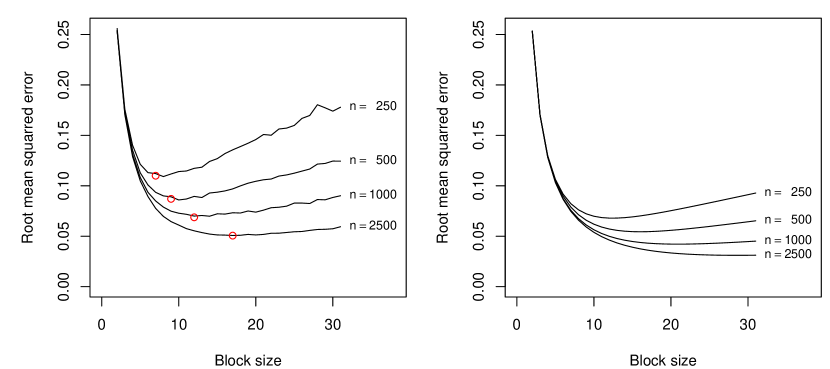
Figure 1: Evolution of the root mean squared error for $\hat{p}_{m}$ (left) and $\hat{p}_{m}^{*}$ (right) as the block size $m$ and the sample size $n$ increase. These estimates were obtained from 2000 Monte-Carlo samples sampled from a Brown–Resnick model with semivariogram $\gamma(h)=h/1.627$. This semivariogram was chosen such that the theoretical extremal concurrence probability is $p=0.5$. The red circles indicate the optimal block sizes as defined by (27) and their corresponding optimal root mean squared error (26).

We first focus only on the sample concurrence probability estimators, i.e., $\hat{p}_{m}$ and $\hat{p}_{m}^{*}$, and analyze their performance with respect to the block size $m$ and the sample size $n$. Based on a Monte-Carlo simulation, Figure 1 shows the evolution of the root mean squared error as the block size grows. As expected, both estimators become increasingly more efficient as the sample size grows and, as seen from (29), the permutation estimator $\hat{p}_{m}^{*}$ is more efficient than $\hat{p}_{m}$—independently of the block size $m$ and the sample size $n$. The circles on the plot indicate the asymptotically optimal block size in (27), which are valid olnly for max-stable data. As expected the observed optimal block sizes are in good agreement with the theoretical ones. In practice, however, since the data are not exactly max-stable, we recommend using slightly larger values of $m$ so as to ensure that the block-maxima are closer to a max-stable model but also to take into account that data usually exhibit serial dependence, e.g., daily observations.

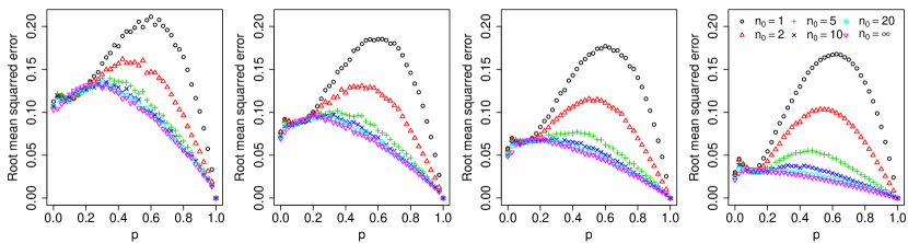
Figure 2: Evolution of the root mean squared error for $\hat{p}$ as the theoretical extremal concurrence probability $p$ and the number of spectral function $n_{0}$ in (35) increase. These estimates were obtained from 2000 Monte-Carlo samples of size $n$ with, from left to right, $n=25,50,100,500$.

We now investigate the performance of the extremal concurrence estimator $\hat{p}$. Figure 2 shows the evolution of the root mean squared error as the number of spectral functions $n_{0}$ in (35) and the theoretical extremal concurrence probability increase. As expected, as the sample size $n$ grows, the estimator $\hat{p}$ becomes much more efficient. Interestingly, for small sample sizes, $\hat{p}$ appears to be fairly robust to the lack of max-stability in the data, i.e., $n_{0}<\infty$. This is not true anymore for larger sample sizes since, as expected, $\hat{p}$ becomes increasingly more efficient as the number of spectral functions increases.

Finally, we compare the performance of the sample concurrence probability estimators $\hat{p}_{m}^{*}$ and $\tilde{p}_{m}^{*}$ with their extremal concurrence counterpart $\hat{p}$. To compare the two types of estimators on a fair basis, we analyze their behaviour when the simulated data are either perfectly max-stable or non max-stable, but in the domain of attraction of a max-stable distribution.

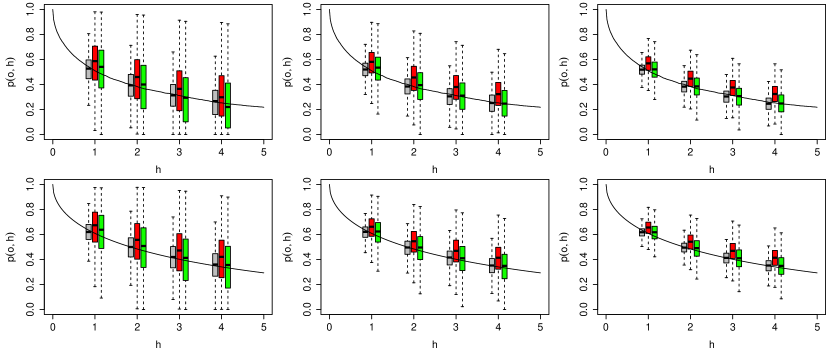
Figure 3: Boxplots of the sample (red / middle), unbiased sample (green / right) and extremal (grey / left) concurrence probability estimators at distance lags $h=1,2,3,4$. The boxplots were obtained from 2000 independent estimates. From left to right: the sample size is respectively 25, 50, 100 and 500. The top panel corresponds to an extremal-$t$ model with $\nu=5$, and correlation function $\rho(h)=\exp(-h/10)$. The bottom panel corresponds to a Brown–Resnick model with semi variogram $\gamma(h)=h/3$. For each panel, the solid line represents the corresponding theoretical extremal concurrence probability function.

Figure 3 shows boxplots of the sample $\hat{p}_{m}^{*}$, unbiased sample $\tilde{p}_{m}^{*}$ and extremal concurrence probability estimators $\hat{p}$, based on 2000 Monte-Carlo realizations of both a Brown–Resnick and extremal-$t$ models. Recall that we focus here on pairwise concurrence probabilities. In this case, the extremal concurrence probability coincides with Kendall’s $\tau$ and therefore, the estimator $\hat{p}$ in (34) is in fact unbiased for the case of max-stable data. This is confirmed by the results in Figure 3. As expected, the variability of all estimators decreases as the sample size grows; the extremal concurrence probability estimator being the most precise one. Since the simulated data are max-stable, we can see that the sample concurrence probability estimator is biased even when the sample size is large while the remaining two estimators are, as expected, unbiased. Overall the extremal concurrence probability appears to be the best estimator provided that the data are max-stable.

Table 1: Performance of the sample $(\hat{p}^{*}_{m})$, unbiased sample $(\tilde{p}^{*}_{m})$ and extremal $(\hat{p})$ concurrence probability estimators. The table report the sample mean and the standard deviation in paren based on 2000 Monte-Carlo replicates. The data are either simulated from an extremal-$t$ model with correlation function $\rho(h)=\exp(-h/10)$ and $\nu=5$ degrees of freedom or from its truncated representation with $n_{0}$ extremal functions. Throughout this simulation study the block size is held fixed to $m=10$, independently of the sample size $n$.

	$p=0.25$				$p=0.50$				$p=0.75$
	$\hat{p}^{*}_{m}$	$\tilde{p}^{*}_{m}$	$\hat{p}$		$\hat{p}^{*}_{m}$	$\tilde{p}^{*}_{m}$	$\hat{p}$		$\hat{p}^{*}_{m}$	$\tilde{p}^{*}_{m}$	$\hat{p}$
Sample size $n=20$
$n_{0}=\phantom{1}1$	$0.41~{}(0.24)$	$0.35~{}(0.26)$	$0.47~{}(0.13)$		$0.64~{}(0.22)$	$0.60~{}(0.24)$	$0.71~{}(0.09)$		$0.83~{}(0.15)$	$0.81~{}(0.17)$	$0.87~{}(0.05)$
$n_{0}=10$	$0.34~{}(0.24)$	$0.27~{}(0.25)$	$0.31~{}(0.14)$		$0.57~{}(0.23)$	$0.52~{}(0.26)$	$0.58~{}(0.12)$		$0.79~{}(0.17)$	$0.77~{}(0.19)$	$0.80~{}(0.07)$
$n_{0}=15$	$0.33~{}(0.24)$	$0.27~{}(0.25)$	$0.30~{}(0.15)$		$0.56~{}(0.23)$	$0.52~{}(0.26)$	$0.56~{}(0.12)$		$0.78~{}(0.17)$	$0.76~{}(0.19)$	$0.78~{}(0.07)$
$n_{0}=\infty$	$0.33~{}(0.24)$	$0.27~{}(0.25)$	$0.25~{}(0.15)$		$0.55~{}(0.24)$	$0.50~{}(0.26)$	$0.50~{}(0.13)$		$0.77~{}(0.18)$	$0.75~{}(0.20)$	$0.75~{}(0.08)$
Sample size $n=50$
$n_{0}=\phantom{1}1$	$0.41~{}(0.13)$	$0.35~{}(0.14)$	$0.47~{}(0.08)$		$0.65~{}(0.10)$	$0.61~{}(0.12)$	$0.71~{}(0.05)$		$0.84~{}(0.07)$	$0.82~{}(0.07)$	$0.87~{}(0.03)$
$n_{0}=10$	$0.34~{}(0.13)$	$0.26~{}(0.14)$	$0.31~{}(0.09)$		$0.57~{}(0.12)$	$0.52~{}(0.13)$	$0.57~{}(0.07)$		$0.79~{}(0.08)$	$0.76~{}(0.09)$	$0.80~{}(0.04)$
$n_{0}=15$	$0.33~{}(0.13)$	$0.25~{}(0.14)$	$0.29~{}(0.09)$		$0.56~{}(0.12)$	$0.51~{}(0.13)$	$0.56~{}(0.07)$		$0.78~{}(0.08)$	$0.76~{}(0.09)$	$0.79~{}(0.04)$
$n_{0}=\infty$	$0.32~{}(0.13)$	$0.25~{}(0.14)$	$0.24~{}(0.09)$		$0.54~{}(0.12)$	$0.49~{}(0.14)$	$0.50~{}(0.08)$		$0.77~{}(0.09)$	$0.74~{}(0.09)$	$0.75~{}(0.05)$
Sample size $n=100$
$n_{0}=\phantom{1}1$	$0.41~{}(0.08)$	$0.35~{}(0.09)$	$0.46~{}(0.06)$		$0.65~{}(0.07)$	$0.61~{}(0.07)$	$0.71~{}(0.03)$		$0.83~{}(0.04)$	$0.82~{}(0.04)$	$0.87~{}(0.02)$
$n_{0}=10$	$0.34~{}(0.09)$	$0.26~{}(0.10)$	$0.31~{}(0.06)$		$0.57~{}(0.08)$	$0.52~{}(0.09)$	$0.57~{}(0.05)$		$0.78~{}(0.05)$	$0.76~{}(0.05)$	$0.80~{}(0.03)$
$n_{0}=15$	$0.33~{}(0.09)$	$0.26~{}(0.10)$	$0.29~{}(0.06)$		$0.56~{}(0.08)$	$0.51~{}(0.09)$	$0.55~{}(0.05)$		$0.78~{}(0.05)$	$0.76~{}(0.06)$	$0.78~{}(0.03)$
$n_{0}=\infty$	$0.33~{}(0.09)$	$0.25~{}(0.10)$	$0.25~{}(0.07)$		$0.55~{}(0.08)$	$0.50~{}(0.09)$	$0.50~{}(0.05)$		$0.78~{}(0.05)$	$0.75~{}(0.06)$	$0.75~{}(0.03)$

To corroborate this finding, Table 1 reports Monte-Carlo sample means and standard deviations of these estimators as the assumption of max-stability becomes more accurate, i.e., as the number $n_{0}$ of spectral functions in (35) grows. As expected, when the max-stability assumption is most unreasonable, i.e., $n_{0}=1$, all estimators show a substantial bias with the extremal concurrence probability estimator $\hat{p}$ having the largest bias while the unbiased sample one $\tilde{p}_{m}^{*}$ the lowest. As the assumption of max-stability becomes increasingly more accurate, the bias of the unbiased sample concurrence and extremal concurrence estimators improve. When this assumption holds exactly (indicated by $n_{0}=\infty$), both of these estimators exhibit essentially no bias as stipulated by the theory and seen in Figure 3. The sample concurrence probability estimator appears to be biased in all situations—the bias being less significant as the number of spectral functions is larger. Interestingly, whatever the estimator considered, the bias and variance appear to increase as the theoretical extremal concurrence probability value $p$ becomes smaller. Overall the extremal concurrence probability estimator $\hat{p}$ in (34) has the lowest variability.

6 Concurrence of temperature extremes in continental USA

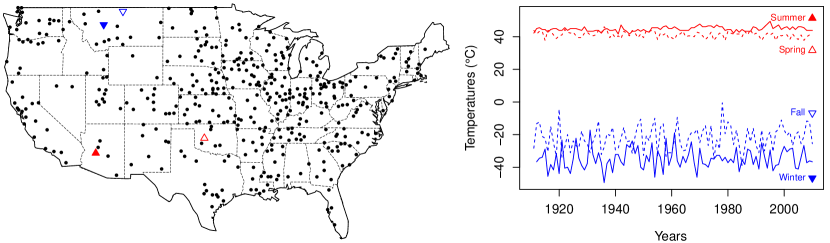
Figure 4: Left: Spatial distribution of the 424 weather stations. The triangles indicate the selected stations for the analysis—upward: daily maxima, downward: daily minima. Right: The seasonal extrema time series of the selected stations.

In this section, we apply the developed methodology to estimate the probabilities of concurrence associated with extreme temperatures—both extreme cold and hot events. The data consists of daily temperature minima and maxima recorded at 424 weather stations over the period 1911–2010. The spatial distribution of these stations is given in Figure 4. This data set, as a subset of the United States Historical Climatological Network USHCN, [2014], was chosen as it meets very high data quality standards and involves fewer than 2.4% missing values while spanning the entire territory of continental US. It can be freely downloaded from http://cdiac.ornl.gov/.

To avoid any seasonal influence on our results we decided to analyze minima and maxima for each season separately. We focus on the concurrence of extreme cold (minima) during the Fall and Winter seasons—generally color-coded in blue; and extreme hot (maxima) during the Spring and Summer seasons—generally color-coded in red. The right panel of Figure 4 shows the times series of these seasonal extrema for four selected weather stations. These stations were selected as they recorded the top seasonal records over the whole spatial and temporal domains. We can see that all four time series of seasonal extremes (cold in blue and hot in red) at these stations appear to be stationary without any clear temporal trend. This is in contrast with the generally accepted trend of about $0.2^{\circ}{\rm C}$ per decade for average temperatures [Stocker et al.,, 2013].

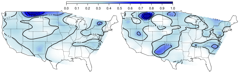
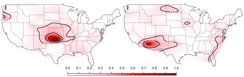
Figure 5: Maps of the extremal concurrence probability for the four selected stations. Top left: Fall (September, October November), top right: Winter (December, January, February), bottom left: Spring (March, April, May) and bottom right: Summer (June, July, August).

Figure 5 plots the estimated spatial distribution of the extremal concurrence probabilities function for each season, relative to the chosen station. More precisely, for a given origin location $s_{0}$, the maps display estimates of the pairwise concurrence probability $p(s_{0},s)$ as a function of $s$. These maps were obtained by first computing the estimator (34) over all $423$ pairs of stations $(s_{0},s)$ and then interpolated using thin plate splines (on logit scale) provided by the R package fields [Nychka et al.,, 2014]. As expected, the highest concurrence probability occurs in the neighbourhood of the selected stations independently of the season. The areal extent of high concurrence probabilities, however, seem to be larger for minimum temperatures (cold extremes) than for maximum temperatures (hot extremes). This finding is consistent with the physical notion of entropy, i.e., when the ambient temperature is higher (Spring and Summer seasons), the entropy is greater and hence involves less spatial dependence than for cooler temperatures leading to smaller probability of simultaneous extremes. This difference can be also attributed to the fact that extreme cold temperatures are often due to high-pressure systems, which tend to linger longer and cover a larger spatial area than warm fronts giving rise to concurrence of extreme hot events.

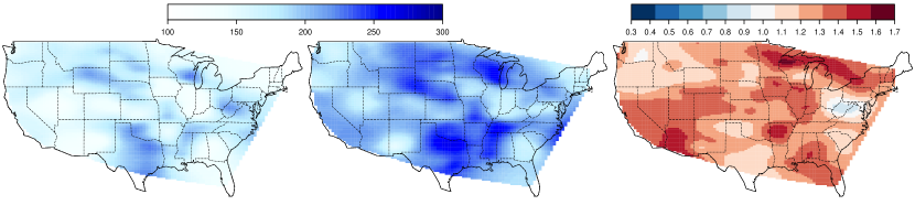
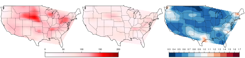
Figure 6: Estimated spatial distribution of the expected extremal concurrence cell areas—in squared degree, i.e., around $1000~{}\mbox{km}^{2}$. From left to right: 1910–1950, 1951–2010, and their ratio (1951–2010 at the numerator). Top: Winter minima, bottom: Summer maxima.

Although Figure 5 displays interesting patterns, it has the drawback of being dependent on the choice of the origin, i.e., the selected station. As stated in Section 5, it is possible to bypass this hurdle by considering the area of concurrence cell. Figure 6 plots the estimated spatial distribution of the concurrence cell area for the preindustrial period, i.e., 1910–1975, and the postindustrial one, i.e., 1976–2010. To emphasize the possible impact of anthropogenic influences, the ratio of these two cell areas is also reported. We can see that during the last sixty years the expected cell area for winter minima have increased of about 30% over the whole USA while there is a decrease of about the same amount for summer maxima. These findings indicates that today’s climate shows cold spells that have a larger impact than in the beginning of the 20th century while hot spells are more localized. Our results agree with the conclusions drawn by Field et al., [2012] who states that “there is evidence from observations gathered since 1950 of change in some extremes”. These changes in the concurrence patterns of summer extremes can be attributed to global warming since an increase in entropy generally leads to more “mixing” in the system and hence less dependence leading to smaller areas of concurrence. The changes in concurrence patterns of extreme cold events, however, are harder to explain. They may be triggered by structural changes in important climatological mechanisms such as the Arctic Oscillation.

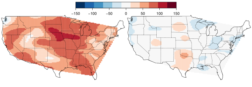
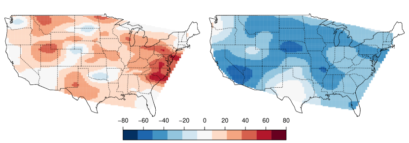
Figure 7: Spatial distribution of the estimated concurrence cell areas anomalies in squared degree, i.e., around $1000~{}\mbox{km}^{2}$ for winter minima (top) and summer maxima (bottom). The data were stratified into three classes: El Niño, La Niña and the base class “La Nada”. The left panels show the anomalies for El Niño, the right ones La Niña.

Finally, we consider another cut of the data by stratifying according to an important climate phenomenon known as the El Niño Southern Oscillation (ENSO). Positive ENSO (El Niño) refers to the event of a warm-up of the surface water in the central and east-central equatorial Pacific ocean. It is well known that years with high ENSO have a general warming effect in North America during the winter season. The opposite effect of negative ENSO (La Niña) is characterized by a cool-down in the same area of the Pacific and it generally leads to unusually cold winters in the northwestern part of the US, northern California and the north-central states Graham, [1999]. Figure 7 shows estimates of concurrence cell areas anomalies for winter minima and summer maxima. These anomalies were defined as pointwise deviations from the expected cell area obtained from La Nada seasons, i.e., neither El Niño nor La Niña seasons. We can see that La Niña does not seem to have an impact on the spatial coverage of winter minima but that El Niño seems to induce more massive cold extremes over the whole USA. For the summer season, La Niña seems to reduce the spatial extent of heat waves over the whole USA while El Niño has a less pronounced impact—although it generally yields larger spatial coverages especially along the East coast.

7 Discussion

In this paper we introduced a new framework for the analysis of dependence of extremes: the extremal/sample concurrence probability. This tool plays a similar role to that of the extremal coefficient but has the benefit, as a probability, of being more interpretable and intuitive. Theoretical properties and closed forms of these concurrence probabilities have been established and several estimators have been proposed. A simulation study has shown that the proposed estimators work well in practice and that they give a new insight about the dependence of extremes, such as the spatial distribution of the expected concurrence cell area of extreme temperature in the continental US.

Appendix A Proofs

A.1 Proof of the continuity of $\Pi$ in Theorem 1

Consider a sequence $\Psi_{n}\to\Psi$ in $\mathscr{M}_{p}([0,\infty]^{k}\setminus\{0\})$ and let $\Psi=\{\psi_{i}\colon i\geq 1\}$ and $\Psi_{n}=\{\psi_{n,i}\colon i\geq 1\}$. As compact subsets of $[0,\infty]^{k}\setminus\{0\}$ are bounded away from $0$, we can choose $\varepsilon>0$ such that

$$\begin{cases}\max_{i\geq 1}\psi_{i}(s_{j})>\varepsilon,&j=1,\ldots,k\\ \psi_{i}(s_{j})\neq\varepsilon,&j=1,\ldots,k,\ i\geq 1.\end{cases}$$

Then $K_{\varepsilon}=[0,\infty]^{k}\setminus[0,\varepsilon)^{k}$ is a compact set, $\Psi\cap K_{\varepsilon}$ has finitely many points $\psi_{1},\ldots,\psi_{N_{\varepsilon}}$ and no point of $\Psi$ lies on the boundary $\partial K_{\varepsilon}$. The convergence $\Psi_{n}\to\Psi$ entails that for $n$ large enough, $\Psi_{n}\cap K_{\varepsilon}$ has the same number of points $\psi_{n,1},\ldots,\psi_{n,N_{\varepsilon}}$ that can be reordered in such a way that $\psi_{n,i}\to\psi_{i}$ as $n\to\infty$, $i=1,\ldots,N_{\varepsilon}$.

Assume that the maxima $\max_{1\leq i\leq N_{\varepsilon}}\psi_{i}(s_{j})$, $j=1,\ldots,k$, are uniquely attained. Then the hitting scenario $\Pi(\Psi)$ is well defined and depends only on $\{\psi_{i}\colon i=1,\ldots,N_{\varepsilon}\}$. By the convergence $\psi_{n,i}\to\psi$, for large $n$ the maxima $\max_{1\leq i\leq N_{\varepsilon}}\psi_{n,i}(s_{j})$ are uniquely attained so that the hitting scenario $\Pi(\Psi_{n})$ is well defined and depends only on $\{\psi_{n,i}\colon i=1,\ldots N_{\varepsilon}\}$. It is not difficult to see (although tedious to write formally) that the convergence $\{\psi_{n,i}\colon i=1,\ldots,N_{\varepsilon}\}\to\{\psi_{i}\colon i=1,\ldots,N_{\varepsilon}\}$ implies $\Pi(\Psi_{n})=\Pi(\Psi)$ for large $n$. This proves the announced continuity for the mapping $\Pi$.

A.2 Proof of Proposition 3

We shall prove below the following formula, which may be of independent interest.

Lemma 2.

In the context of Proposition 3, we have

$$p_{m}=p+\sum_{\ell=2}^{k}\mathbb{P}(|\pi|=\ell)m^{1-\ell}$$ (36)

where $\pi$ is the extremal hitting scenario and $|\pi|$ its number of components.

Proposition 3 follows directly from (36). Indeed, the monotonicity of $p_{m}$ is immediate and since $p=\mathbb{P}(|\pi|=1)$, we have

$$0\leq p_{m}-p=\sum_{\ell=2}^{k}\frac{\mathbb{P}(|\pi|=\ell)}{m^{\ell-1}}\leq\frac{1}{m}\sum_{\ell=2}^{k}\mathbb{P}(|\pi|=\ell)=\frac{(1-p)}{m}.$$

If $p<1$, then at least one of the probabilities $\mathbb{P}(|\pi|=\ell)$, $\ell=2,\ldots,k$ is non-zero and by (36) the asymptotic equivalence $(p_{m}-p)\sim c_{r}/m^{r}$, $m\to\infty$ holds where $r\in\{1,\ldots,k-1\}$ is the smallest integer, such that $c_{r}=\mathbb{P}(|\pi|=r+1)>0$.

Proof of Lemma 2.

Since $Z_{1},\ldots,Z_{m}$ are independent with the same distribution as $\eta$, we can suppose from (5) that

$$Z_{i}(s)=\max_{\phi\in\Phi_{i}}\phi(s),\qquad s\in\mathcal{X},$$

with $\Phi_{1},\ldots,\Phi_{m}$ independent copies of $\Phi$. By max-stability, $\bar{\eta}=m^{-1}\max_{1\leq i\leq m}Z_{i}$ has the same distribution as $\eta$ and $\bar{\Phi}=\cup_{1\leq i\leq m}\{m^{-1}\phi,\phi\in\Phi_{i}\}$ has the same distribution as $\Phi$. We consider the following events

$$A =\{\text{sample concurrence occurs for $Z_{1},\ldots,Z_{m}$}\}$$

$$B =\{\text{extremal concurrence occurs for $\bar{\eta}$}\}$$

Clearly, $\mathbb{P}(A)=p_{m}$ and $\mathbb{P}(A)=\mathbb{P}(A\cap B)+\mathbb{P}(A\cap B^{c})$ with $B^{c}$ the complementary set of $B$. We analyze the two terms separately.

Observe first that if extremal concurrence occurs then we also have sample concurrence. Indeed, if $B$ occurs, then one function of $\bar{\Phi}$ dominates all the others at $(s_{1},\ldots,s_{k})$. This function is of the form $m^{-1}\phi$ with $\phi\in\Phi_{i}$, for some $i=1,\ldots,m$, showing that $Z_{i}$ dominates $Z_{1},\ldots,Z_{m}$, i.e., we have sample concurrence. Hence $B\subset A$ and $\mathbb{P}(A\cap B)=\mathbb{P}(B)=p$. We now consider the second term and the event $A\cap B^{c}$, i.e., sample concurrence occurs in $Z_{1},\ldots,Z_{m}$ but not extremal concurrence for $\bar{\eta}$. Let $\bar{\pi}$ be the hitting scenario of $\bar{\eta}$. We know that $B^{c}$ is equivalent to $|\bar{\pi}|\geq 2$, i.e. the maximum at locations $(s_{1},\ldots,s_{k})$ is attained by at least two functions in $\bar{\Phi}$. These functions are of the form $m^{-1}\phi_{j}$, $1\leq j\leq\ell$, with $\ell=|\bar{\pi}|$ and $\phi_{j}\in\Phi_{i_{j}}$ for some $1\leq i_{j}\leq m$. If $A$ is also realized, i.e., some $Z_{i}$ dominates $Z_{1},\ldots,Z_{m}$, then we must have $i_{1}=\cdots=i_{\ell}=i$. Note, however, that since the point processes $\Phi_{i}$, $i=1,\ldots,m$ are independent and identically distributed, any given function $m^{-1}\phi\in\bar{\Phi}\equiv\cup_{i=1}^{m}m^{-1}\Phi_{i}$, independently from the others, has equal chance of coming from any one of the $m$ point processes $m^{-1}\Phi_{i}$, $i=1,\ldots,m$. Therefore, the probability that all $\ell$ functions contributing to the maximum at sites $(s_{1},\ldots,s_{k})$ are assigned to component $i$ is $m^{-\ell}$. Since there are $m$ possible choices for the index $i$, we deduce

$$\mathbb{P}(A\cap B^{c})=\sum_{\ell=2}^{k}\mathbb{P}(|\bar{\pi}|=\ell)m^{1-\ell}.$$

Equation (36) follows. ∎

A.3 Proofs of Theorems 5 and 6

In the context of these two theorems, we have

$$p_{m}-p\sim c_{r}m^{-r},\qquad m\to\infty,$$ (37)

for some $r\in\{1,\ldots,k-1\}$ and $c_{r}>0$—cf. Proposition 3. Let $S_{n}=[n/m]\hat{p}_{m}=\sum_{i=1}^{[n/m]}\xi_{i,n}$, where $\xi_{i,n}$ are iid Bernoulli$(p_{m})$.

Proof of Theorem 5.

Let $B_{n}={\rm Var}(S_{n})=[n/m]p_{m}(1-p_{m})$ and introduce the cumulative distribution function

$$F_{n}(x)=\mathbb{P}\left[B_{n}^{-1/2}\{S_{n}-\mathbb{E}(S_{n})\}\leq x\right]\equiv\mathbb{P}\left\{\sqrt{\frac{[n/m]}{p_{m}(1-p_{m})}}(\hat{p}_{m}-p_{m})\leq x\right\},\qquad x\in\mathbb{R}.$$

The Berry–Essen theorem (see e.g. Theorem V.2.3 in Petrov, [1975]) implies that

$$\sup_{x\in\mathbb{R}}|F_{n}(x)-\Phi(x)|\leq AL_{n},$$ (38)

where $A$ is an absolute constant, $\Phi(x)$ denotes the standard Normal cumulative distribution function and

$$L_{n}=B_{n}^{-3/2}\sum_{i=1}^{[n/m]}\mathbb{E}\left(|\xi_{i,n}-p_{m}|^{3}\right).$$

Using that $\mathbb{E}(|\xi_{i,n}-p_{m}|^{3})\leq p_{m}(1-p_{m})$ and straightforward algebra, we obtain

$$L_{n}\leq\left[(n/m)p_{m}(1-p_{m})\right]^{-1/2}.$$ (39)

Since $0<p<1$, we have $p_{m}(1-p_{m})\sim p(1-p)>0$ as $n\to\infty$ and, for an arbitrary choice of $m=m(n)=o(n)$ as $n\to\infty$, we have $L_{n}\to 0$. This, in view of (38) yields

$$\sqrt{n/m}(\hat{p}_{m}-p_{m})\longrightarrow N\{0,p(1-p)\}.$$ (40)

By using (37) and Slutsky’s theorem, we obtain the final result. ∎

Proof of Theorem 6.

In case $\lambda<\infty$, since $p=0$, from (37), we have $p_{m}\sim c_{r}/m^{r},\ n\to\infty$, and hence

$$[n/m]p_{m}\sim c_{r}n/m^{(r+1)}\longrightarrow c_{r}/\lambda^{(r+1)},\qquad n\to\infty.$$ (41)

Thus, the standard Poisson convergence for the Binomial$(p_{m},[n/m])$ random variables $S_{n}=[n/m]\hat{p}_{m}$ yields the result.

When $\lambda=\infty$, by (41), we have $x_{n}=[n/m]p_{m}\to 0$ as $n\to\infty$. Therefore,

$$\mathbb{P}(\hat{p}_{m}=0)=(1-p_{m})^{[n/m]}=\left(1-\frac{x_{n}}{[n/m]}\right)^{[n/m]}\sim\exp(-x_{n})\longrightarrow 1,\qquad n\to\infty,$$

which completes the proof. ∎

References

- Cooley et al., [2006] Cooley, D., Naveau, P., and Poncet, P. (2006). Variograms for spatial max-stable random fields. In Bertail, P., Soulier, P., Doukhan, P., Bickel, P., Diggle, P., Fienberg, S., Gather, U., Olkin, I., and Zeger, S., editors, Dependence in Probability and Statistics, volume 187 of Lecture Notes in Statistics, pages 373–390. Springer New York.
- Davison et al., [2012] Davison, A., Padoan, S., and Ribatet, M. (2012). Statistical modelling of spatial extremes. Statistical Science, 7(2):161–186.
- de Haan, [1984] de Haan, L. (1984). A spectral representation for max-stable processes. The Annals of Probability, 12(4):1194–1204.
- Dengler, [2010] Dengler, B. (2010). On the asymptotic behavior of Kendall’s Tau. PhD thesis, Vienna University of Technology, Vienna, Austria. http://www.ub.tuwien.ac.at/diss/AC07806793.pdf.
- Dombry and Éyi-Minko, [2013] Dombry, C. and Éyi-Minko, F. (2013). Regular conditional distributions of max infinitely divisible random fields. Electronic Journal of Probability, 18(7):1–21.
- Dombry et al., [2013] Dombry, C., Éyi-Minko, F., and Ribatet, M. (2013). Conditional simulations of max-stable processes. Biometrika, 100(1):111–124.
- Dombry and Kabluchko, [2014] Dombry, C. and Kabluchko, Z. (2014). Random tessellations associated with max-stable random fields. ArXiv. Preprint. http://arxiv.org/abs/1410.2584v2.
- Field et al., [2012] Field, C., Barros, V., Stocker, T., Qin, D., Dokken, D., Ebi, K., Mastrandrea, M., Mach, K., Plattner, G.-K., Allen, S., Tignor, M., and Midgley, P., editors (2012). IPCC, 2012: Managing the Risks of Extreme Events and Disasters to Advance Climate Change Adaptation. A Special Report of Working Groups I and II of the Intergovernmental Panel on Climate Change. Cambridge University Press, Cambridge University Press, Cambridge, UK, and New York, NY, USA.
- Ghoudi et al., [1998] Ghoudi, K., Khoudraji, A., and Rivest, L.-P. (1998). Propriétés statistiques des copules de valeurs extrêmes bidimensionnelles. Canad. J. Statist., 26(1):187–197.
- Graham, [1999] Graham, S. (1999). NASA: Earth Observatory. Web resource: http://earthobservatory.nasa.gov/Features/LaNina/.
- Kabluchko, [2009] Kabluchko, Z. (2009). Spectral representations of sum- and max-stable processes. Extremes, 12(4):401–424.
- Kabluchko et al., [2009] Kabluchko, Z., Schlather, M., and de Haan, L. (2009). Stationary max–stable fields associated to negative definite functions. Annals of Probability, 37(5):2042–2065.
- Nychka et al., [2014] Nychka, D., Furrer, R., and Sain, S. (2014). fields: Tools for spatial data. R package version 7.1.
- Penrose, [1992] Penrose, M. D. (1992). Semi-min-stable processes. Annals of Probability, 20(3):1450–1463.
- Petrov, [1975] Petrov, V. V. (1975). Sums of independent random variables. Springer-Verlag, New York-Heidelberg. Translated from the Russian by A. A. Brown, Ergebnisse der Mathematik und ihrer Grenzgebiete, Band 82.
- Resnick, [1987] Resnick, S. I. (1987). Extreme Values, Regular Variation and Point Processes. Springer-Verlag, New York.
- Samorodnitsky and Taqqu, [1994] Samorodnitsky, G. and Taqqu, M. S. (1994). Stable Non-Gaussian Processes: Stochastic Models with Infinite Variance. Chapman and Hall, New York, London.
- Schemper, [1987] Schemper, M. (1987). Nonparametric estimation of variance, skewness and kurtosis of the distribution of a statistic by jackknife and bootstrap techniques. Statist. Neerlandica, 41(1):59–64.
- Schlather, [2002] Schlather, M. (2002). Models for stationary max-stable random fields. Extremes, 5(1):33–44.
- Schlather and Tawn, [2003] Schlather, M. and Tawn, J. (2003). A dependence measure for multivariate and spatial extremes: Properties and inference. Biometrika, 90(1):139–156.
- Smith, [1990] Smith, R. L. (1990). Max-stable processes and spatial extreme. Unpublished manuscript.
- Stocker et al., [2013] Stocker, T., , Qin, D., Plattner, G.-K., Tignor, M., Allen, S., Boschung, J., Nauels, A., Xia, Y., Bex, V., and Midgley, P., editors (2013). IPCC, 2013: Climate Change 2013: The Physical Science Basis. Contribution of Working Group I to the Fifth Assessment Report of the Intergovernmental Panel on Climate Change. Cambridge University Press, Cambridge, United Kingdom and New York, NY, USA.
- Stoev and Taqqu, [2005] Stoev, S. and Taqqu, M. S. (2005). Extremal stochastic integrals: a parallel between max–stable processes and stable processes. Extremes, 8:237–266.
- Stoev, [2008] Stoev, S. A. (2008). On the ergodicity and mixing of max-stable processes. Stochastic Process. Appl., 118(9):1679–1705.
- USHCN, [2014] USHCN (2014). United States Historical Climatological Network: Daily temperature extremes for the period 1911–2010 in continental USA. Data resource: http://cdiac.ornl.gov/ftp/us_recordtemps/sta424/.
- Wang and Stoev, [2011] Wang, Y. and Stoev, S. A. (2011). Conditional sampling for spectrally discrete max-stable random fields. Advances in Applied Probability, 443:461–483.
- Weintraub, [1991] Weintraub, K. S. (1991). Sample and ergodic properties of some min–stable processes. The Annals of Probability, 19(2):706–723.