Long-term behavior of reaction-diffusion equations with nonlocal boundary conditions on rough domains

Abstract.

We investigate the long term behavior in terms of finite dimensional global and exponential attractors, as time goes to infinity, of solutions to a semilinear reaction-diffusion equation on non-smooth domains subject to nonlocal Robin boundary conditions, characterized by the presence of fractional diffusion on the boundary. Our results are of general character and apply to a large class of irregular domains, including domains whose boundary is Hölder continuous and domains which have fractal-like geometry. In addition to recovering most of the existing results on existence, regularity, uniqueness, stability, attractor existence, and dimension, for the well-known reaction-diffusion equation in smooth domains, the framework we develop also makes possible a number of new results for all diffusion models in other non-smooth settings.

1. Introduction

The mathematical theory for global existence and regularity of solutions to the (scalar) reaction-diffusion equation is considered a central problem in understanding models of (non-)degenerate reaction-diffusion systems for a variety of applied problems, especially in chemistry and biology. It is also essential, for practical applications, to be able to understand, and even predict, the long time behavior of the solutions of such systems. It is well-known that the asymptotic behavior of solutions to (scalar) reaction-diffusion equations can be well described by invariant attracting sets, and, in particular, by a finite-dimensional global attractor, such that, the dynamics of these equations, when restricted to these sets, is effectively described by a finite number of parameters (see, e.g., the monographs [10, 16, 51, 53]).

Analytical results for most PDEs in the literature nowadays revolve around the most commonly found assumption that the underlying physical space $\Omega\subset{\mathbb{R}}^{N}$ ($N\geq 2$) is smooth enough, and that at best, the boundary of $\Omega$, $\partial\Omega$ is of Lipschitz class. But this is barely non-smooth, since a Lipschitz boundary has a tangent plane almost everywhere. On the other hand, not much seems to be known about partial differential equations (except for some scarce results which we will describe below) and their long-time behavior in general, when the physical domain $\Omega$ is actually ”rough”. This is the case, for instance, of domains whose boundary has either a fractal-like geometry or domains with cusps which are also frequently used in the applications. Indeed, it cannot be expected that objects in the real-world, be they are clouds, trees, snowflakes, blood vessels, etc., will possess the structure of smooth manifolds [44]. One of the main technical difficulties nowadays of dealing with ”bad” domains is the scarcity of Sobolev embedding theorems and interpolation results in this general context. In fact, for a general non-smooth domain the usual Sobolev embedding and density theorems do not hold [49] (cf. also Section 2).

Our main goal in this paper is to develop well-posedness and long-time dynamics results for reaction-diffusion equations on domains $\Omega$ with ”rough” boundaries, and then subsequently recover the existing results of this type for the same models that have been previously obtained in the case of domains with smooth boundary $\partial\Omega$. Along these lines, we first establish a number of results for scalar reaction-diffusion equations, including results on existence, regularity, uniqueness of weak and strong solutions, existence and finite dimensionality of global and exponential attractors, and existence of Lyapunov functions. To be more precise, we shall be concerned with diffusion processes in ”rough” domains $\Omega$, described by the equation

$$\partial_{t}u-\Delta u+f\left(u\right)=0\text{ in }\Omega\times\left(0,\infty\right),$$ (1.1)

subject to the following nonlocal Robin boundary condition

$$\partial_{\nu}ud\sigma+(u+\Theta_{\mu}\left(u\right))d\mu=0\text{ on }\partial\Omega\times\left(0,\infty\right),$$ (1.2)

and the initial condition

$$u\left(0\right)=u_{0}\text{ in }\Omega.$$ (1.3)

In Eqn. (1.1), $f=f\left(u\right)$ plays the role of nonlinear source, not necessarily monotone, and $\Theta_{\mu}\left(u\right)$ is a certain nonlocal operator characterizing the presence of ”fractional” diffusion along $\partial\Omega$ (see Eq. (2.7) below). The normal derivative $\partial_{\nu}u$ is understood in the sense of (1.4) specified below, $\sigma$ denotes the restriction to $\partial\Omega$ of the $(N-1)$-dimensional Hausdorff measure $\mathcal{H}^{N-1}$, $\mu$ is an appropriate positive regular Borel measure on $\partial\Omega$. In fact, the regularity assumptions we will impose on $\partial\Omega$ enter through the measure $\mu$ in (1.2). We will make this more precise in Section 2. Since for a ”rough” domain $\Omega$ the boundary $\partial\Omega$ may be so irregular that no normal vector can be defined, we will use the following generalized version of a normal derivative in the weak sense introduced in [13]. Let $\mu$ be again a Borel measure on $\partial\Omega$ and let $F:\Omega\rightarrow{\mathbb{R}}^{N}$ be a measurable function. If there exists a function $f\in L_{loc}^{1}({\mathbb{R}}^{N})$ such that

$$\int_{\Omega}F\cdot\nabla\varphi dx=\int_{\Omega}f\varphi dx+\int_{\partial\Omega}\varphi d\mu$$ (1.4)

for all $\varphi\in C^{1}(\overline{\Omega})$, then we say that $\mu$ is the normal measure of $F$ which we denoted by $N^{\star}(F):=\mu$. If $N^{\star}(F)$ exists, then it is unique and $dN^{\star}(\psi F)=\psi dN^{\star}(F)$ for all $\psi\in C^{1}(\overline{\Omega})$. If $u\in W_{loc}^{1,1}(\Omega)$ and $N^{\star}(\nabla u)$ exists, then we will denote by $N(u):=N^{\star}(\nabla u)$ the generalized normal measure of $\nabla u$. The derivative $dN(u)/d\sigma$ that we denote by $\partial_{\nu}u$ will be called the generalized normal derivative of $u$. To justify this definition, consider the special case of a bounded domain $\Omega\subset{\mathbb{R}}^{N}$ whose boundary is Lipschitz continuous, $\nu$ the outer normal to $\partial\Omega$ and let $\sigma$ be the (natural) surface measure on $\partial\Omega$ (in this case, $\sigma$ also coincides with $\mathcal{H}_{\mid\partial\Omega}^{N-1}$). If $u\in C^{1}(\overline{\Omega})$ is such that there are $f\in L_{loc}^{1}({\mathbb{R}}^{N})$ and $g\in L^{1}(\partial\Omega,\sigma)$ with

$$\int_{\Omega}\nabla u\cdot\nabla\varphi dx=\int_{\Omega}f\varphi dx+\int_{\partial\Omega}g\varphi d\sigma$$

for all $\varphi\in C^{1}(\overline{\Omega})$, then $dN(u)=gd\sigma$ with $g=\partial_{\nu}u=\partial u/\partial\nu$. Throughout the following, without any mention, for a bounded arbitrary domain $\Omega,$ we will always mean the identity (1.4) for the generalized outer normal derivative of $u$.

The interest in analysis and modelling of diffusion processes in bounded domains whose (part of the) boundary possess a fractal geometry arises from mathematical physics, and dates back to the early 1980’s. The first analytical results aimed at understanding transmission problems, which, in electrostatics and magnetostatics, describe heat transfer through a fractal-like interface (such as, the snowflake), can be found in [39, 40, 41, 42]. The type of parabolic problems we consider also occur in the field of the so-called “hydraulic fracturing”, a frequently used engineering method to increase the flow of oil from a reservoir into a producing oil well (see [14]; cf. also [36] for a related application). Further examples are also provided in the book of Dautray and Lions [22]. In all these applications, the mathematical model is usually a linear parabolic boundary value problem involving a transmission condition on a fractal-like interface (layer) which is often a Robin boundary condition. The reaction-diffusion equation (1.1) on unbounded fractal domains has also been considered in [27], and in [35], for bounded fractal domains for which the usual Sobolev-type inequalities hold and for which (1.1) is equipped with homogeneous Dirichlet boundary conditions on $\partial\Omega$. The latter contributions devote their attention mainly to some existence results for some special cases of nonlinearities. The motivation to consider (1.1)-(1.3) is also inspired by a wider and challenging problems aimed at simulating the diffusion of e.g. medical sprays in the bronchial tree [46, 47]. In this case, the geometry of the underlying physical domain can be simulated by some classes of self-similar ramified domains with a fractal boundary. Oxygen diffusion between the lungs and the circulatory system takes place only in the last generations of the lung tree, so that a reasonable diffusion model may need to involve nonlocal Robin boundary conditions (1.2) on the top boundary (the smallest structures), see Section 2 (cf. also [2, 3, 4]).

It would be extremely useful if one could give a unified analysis of the reaction-diffusion problem (1.1)-(1.3) for a large class of rough domains, including the specified families of ”fractal” domains and/or domains with cusps, using only a minimal number of regularity properties for $\Omega$, and then use these assumptions about the specific form of the domain, leading to specific models, to derive sharp results about existence, regularity and stability of solutions. Then, it is also essential, for further practical applications, to show the existence of the global attractor for our general model, and then to determine whether the dynamics restricted to this global attractor is finite-dimensional or not. Among the first important contributions made to understand the linear problem associated with Eqns. (1.1)-(1.2), in general bounded open sets $\Omega$ with no essential regularity assumptions on $\partial\Omega,$ can be found in [59] (cf. also [54] for related results). In particular, in [59] it is shown that the unique solution of the linear problem is given in terms of a strongly continuous (linear) semigroup of contraction operators on $L^{2}\left(\Omega\right),$ that is order preserving, nonexpansive on $L^{\infty}\left(\Omega\right)$, and ultracontractive (see Section 2; cf. also [59, Sections 3-5]). The first tool used to derive this result is the validity of the following inequality, for arbitrary open sets $\Omega$ with finite measure,

$$\|u\|_{L^{\frac{2N}{N-1}}\left(\Omega\right)}\leq C_{\Omega}\left(\|\nabla u\|_{L^{2}\left(\Omega\right)}+\|u\|_{L^{2}(\partial\Omega,\sigma)}\right),$$ (1.5)

which holds for any $u\in W^{1,2}(\Omega)\cap C_{c}(\overline{\Omega})$, for some $C_{\Omega}=C(N,\Omega)>0$. This crucial inequality is due to Maz’ya [49]. We recall that for Lipschitz domains, the optimal exponent on the left-hand side of (1.5) is $2N/\left(N-2\right),$ while for arbitrary open domains $\Omega,$ the best optimal exponent is $2N/\left(N-1\right)$, see Section 2.2. The second tool is the notion of relative capacity with respect to $\Omega$ [8, 9], which is a fundamental tool both in classical analysis and potential theory. Its most common property is that it measures small sets more precisely than the usual Lebesgue measure. With both these tools at disposal, the local Robin boundary condition (that is, $\Theta_{\mu}\equiv 0$ in Eqn. (1.2)) for the linear heat equation has been investigated in [12, 13] (and the references therein) under the stronger restriction that $\Omega$ possesses the extension property of Sobolev functions. The (linear) elliptic system associated with equations (1.1)-(1.2) has also been considered in [8, 9, 18, 19, 20], also without any essential regularity assumptions on $\Omega$. These latter references are mainly concerned with the existence of weak solutions for these elliptic systems and several apriori estimates.

In addition to deriving well-posedness and regularity results for our nonlinear model, perhaps the study of the asymptotic behavior is equally as important as it is essential to be able to understand, and even predict, the long time behavior of the solutions of our system. One object well-suited to describe the long-time behavior is the global attractor. Assuming $f\in C_{\text{loc}}^{1}\left(\mathbb{R}\right)$ is a function which satisfies, for appropriate positive constants,

$$C_{f}\left|s\right|^{p}-c_{f}\leq f\left(s\right)s\leq\widetilde{C}_{f}\left|s\right|^{p}+\widetilde{c}_{f},\text{ }p>1$$ (1.6)

and

$$f^{{}^{\prime}}\left(s\right)\geq-C_{f},\text{ for all }s\in\mathbb{R}\text{,}$$ (1.7)

resembling the same classical assumptions (see, e.g., [16, 51]), we prove in Section 3.2 that (1.1)-(1.3) generates a nonlinear continuous semigroup $\left\{\mathcal{S}\left(t\right)\right\}_{t\geq 0}$ acting on the phase space $L^{2}\left(\Omega\right)$ (see Corollary 3.9). This semigroup possesses the global attractor $\mathcal{G}_{\Theta,\mu}$, which is compact in $L^{2}\left(\Omega\right)$, bounded in $L^{\infty}\left(\Omega\right)$ and has finite fractal dimension (see Corollary 4.8). In addition, we show that every unique orbit $u\left(t\right)=\mathcal{S}\left(t\right)u_{0},$ $u_{0}\in L^{2}\left(\Omega\right)$, of the parabolic problem (1.1)-(1.3) ”instantaneously” exhibits an improved regularity both in space and time. More precisely, every such weak solution becomes a strong solution (see Section 3.3); hence, $\mathcal{G}_{\Theta,\mu}$ contains only strong solutions. In fact, the aim of the whole Section 3.1 is to verify the existence of (unique) strong solutions which are smooth enough (even with more general assumptions than (1.6)-(1.7)). One of the advantages of this result is that every weak solution can be approximated by the strong ones and the rigorous justification of the regularity results for such solutions becomes immediate. In particular, exploiting Maz’ya inequality (1.5) we extend the scheme developed initially by Alikakos [7] for reaction-diffusion equations, to derive that a particular smoothing property holds for all weak solutions of (1.1)-(1.3) with a function $f$ satisfying (1.6)-(1.7). Here we emphasize again that the original proofs due to Alikakos [7] rely heavily on the application of the Gagliardo-Nirenberg-Sobolev inequality which unfortunately is no longer valid in our context. Besides, in our iteration scheme we need to get good control of certain constants in such a way that they do not depend on (the bad behavior of) $\partial\Omega$. Furthermore, a key point of this analysis is to employ an appropriate fixed point argument, coupled together with a hidden regularity theorem (Appendix, Theorem 6.3) for a non-autonomous equation governed by an accretive operator, to deduce smooth strong solutions which are differentiable almost everywhere on $\left(0,\infty\right)$. This regularity is crucial to show, for instance, that problem (1.1)-(1.3) has a Lyapunov function on the global attractor $\mathcal{G}_{\Theta,\mu}$ (see Lemma 4.3 and Theorem 4.5). Clearly, $\mathcal{G}_{\Theta,\mu}$ depends on the choice of boundary conditions (1.2) and the measure $\mu$ on $\partial\Omega$ (see, for instance, Theorems (A) and (B) below). At this point one could argue that the long-time behavior of system (1.1)-(1.3) is properly described by the global attractor. However, it is well-known that the global attractor can present several drawbacks, among which we can mention that it may only attract the trajectories at a slow rate, and that the rate of attraction is very difficult, if not impossible, to express in terms of the physical observable quantities (see, e.g., [50]). Furthermore, in many situations, the global attractor may not be even observable in experiments or in numerical simulations. This can be seen, for instance, for the one-dimensional Chaffee-Infante equation

$$\partial_{t}u-d\partial_{x}^{2}u+f\left(u\right)=0$$

on the interval $(0,1)$, with cubic nonlinearity $f\left(s\right)=s^{3}-s,$ and non-homogeneous Dirichlet boundary conditions (i.e., $u\left(0,t\right)=u\left(1,t\right)=-1$, $t>0$), in which case every trajectory is exponentially attracted to the ”single point” attractor $\left\{-1\right\}$. On the other hand, this problem possesses many interesting metastable “almost stationary” equilibria which live up to a time $t_{\ast}\sim e^{d^{-1/2}}$ and, thus, for $d>0$ small, one will not see the global attractor in numerical simulations. This is known to happen, for instance, for some models of one-dimensional Burgers equations and models of pattern formation in chemotaxis (see [50], for further references). Henceforth, in some situations, the global attractor may fail to capture important transient behaviors. Besides, in the general setting of arbitrary open domains, this feature can be further amplified for our system due to the boundary condition (1.2) and the ”rough” nature of the domain $\Omega$ near $\partial\Omega$. It is thus also important to construct larger objects which contain the global attractor, attract the trajectories at a fast (typically, exponential) rate which can be computed explicitly in terms of the physical parameters, and are still finite dimensional. A natural object is the exponential attractor (see, e.g., [50, Section 3]; cf. also below). In Section 4, we prove the existence of such an exponential attractor not only for the dynamical systems generated by the weak solutions (see Theorem 4.7) but also by the strong solutions, which require essentially no growth assumptions on the nonlinearity as $\left|s\right|\rightarrow\infty$ (see Theorem 4.11). Roughly speaking, the assumption on $f$ reads:

$$\liminf_{\left|s\right|\rightarrow+\infty}\frac{f\left(s\right)}{s}>-\lambda_{\ast},$$ (1.8)

for some $\lambda_{\ast}\in[0,C_{\Omega})$, where $C_{\Omega}=C\left(N,\Omega\right)>0$ is the best Sobolev/Poincaré constant into (1.5). The latter result seems to be new for (1.1)-(1.3) even when $\Omega$ is a smooth domain. We refer the reader to Section 3 for the precise assumptions, related results and generalizations.

We emphasize that the measure $\mu$ and/or boundary regularity assumptions we employ are of general character, and as a result do not require any specific form of the domain $\Omega$; this abstraction allows (1.1)-(1.3) to recover all of the existing diffusion models that have been previously studied in smooth bounded domains (including Lipschitz domains), as well as to represent a much larger family of models for (1.1)-(1.3) that have not been explicitly studied in detail. As a result, the system in (1.1)-(1.3) includes reaction-diffusion models, on domains $\Omega$ which possess the $W^{1,2}$-extension property of Sobolev functions, and non-Lipschitz domains whose boundary is only Hölder continuous, as special cases, and on many arbitrary open bounded domains $\Omega$ (satisfying, for instance, (1.5)) not previously identified. In Section 5, we discuss how the unified analysis presented here can be used to establish the same results for other important classes of partial differential equations, such as, reaction-diffusion systems for a vector-valued function $\overrightarrow{u}=\left(u_{1},...,u_{k}\right).$

The following theorems can be treated as special cases of our results. They apply for instance to domains $\Omega$ with a ”fractal” boundary $\partial\Omega.$

Theorem (A).

Assume that $\Omega$ has the $W^{1,2}$-extension property of Sobolev functions and $f$ satisfies (1.6)-(1.7). Let $\mu$ be the restriction to $\partial\Omega$ of the $d$-dimensional Hausdorff measure $\mathcal{H}^{d},$ for any $d\in\left(N-2,N\right)$. Then, the dynamical system $\mathcal{S}\left(t\right):L^{2}\left(\Omega\right)\rightarrow L^{2}\left(\Omega\right)$, $u_{0}\mapsto u\left(t\right)=\mathcal{S}\left(t\right)u_{0},$ associated with weak solutions for the parabolic problem (1.1)-(1.3) is gradient-like and possesses the global attractor $\mathcal{G}_{\Theta,\mu}$ of finite fractal dimension. Moreover, the semigroup $\mathcal{S}\left(t\right)$ also has an exponential attractor $\mathcal{E}_{\Theta,\mu}.$

Theorem (B).

Assume that $\Omega$ has the $W^{1,2}$-extension property of Sobolev functions and $f$ obeys (1.8). Let $\mu$ be the restriction to $\partial\Omega$ of the $d$-dimensional Hausdorff measure $\mathcal{H}^{d},$ for any $d\in\left(N-2,N\right)$. Then, the dynamical system $\mathcal{T}\left(t\right):L^{\infty}\left(\Omega\right)\rightarrow L^{\infty}\left(\Omega\right)$, $u_{0}\mapsto u\left(t\right)=\mathcal{T}\left(t\right)u_{0},$ associated with ”strong” solutions of the parabolic problem (1.1)-(1.3) has an exponential attractor $\mathcal{Y}_{\Theta,\mu}$ (hence, also a global attractor of finite fractal dimension).

The assumption on the measure $\mu$ deserves some additional comments. First, we note that when $d=N-1$ but $\mu=\mathcal{H}_{\mid\partial\Omega}^{N-1}\left(=\sigma\right)$ is locally infinite, that is, for all $x\in\partial\Omega$ and $\delta>0$ we have that

$$\sigma\left(B_{\delta}\left(x\right)\cap\partial\Omega\right)=\infty,$$ (1.9)

in this case the boundary value problem (1.1)-(1.2) coincides with the (homogeneous) Dirichlet problem for (1.1). If (1.9) only holds on part of the boundary $\Gamma_{\infty}\subset\partial\Omega$, Dirichlet boundary conditions are satisfied on that part $\Gamma_{\infty}$ and the usual (nonlocal) Robin boundary condition (1.2) is satisfied on the remaining part $\partial\Omega\backslash\Gamma_{\infty}$. On the other hand, for domains with fractal boundaries $\partial\Omega$, one often finds some $d_{0}\in\left(N-2,N\right)$ such that

$$\mu_{d_{0}}=\mathcal{H}_{\mid\partial\Omega}^{d_{0}}\text{ and }\mu_{d_{0}}\left(\partial\Omega\right)<\infty.$$

In this case, one may think of (1.2) as a generalized (nonlocal) Robin boundary condition ($\mu=\mu_{d_{0}}$) for the boundary value problem (1.1)-(1.3). We once again refer the reader to Section 4 for more precise statements of the results on the existence of finite dimensional global and exponential attractors.

The remainder of the paper is structured as follows. In Section 2, we establish our notations and give some basic preliminary results for the operators and spaces appearing in the model (1.1)-(1.3). In Section 3, we prove some well-posedness results for this model; in particular, we establish existence results for strong solutions (Section 3.1), weak solutions (Section 3.2) and then derive regularity (Section 3.3) and stability results (Section 3.2). In Section 4, we prove results which establish the existence of global and exponential attractors for (1.1)-(1.3), and the existence of Lyapunov functions. Section 5 contains some concluding remarks. To make the paper reasonably self-contained, in Appendix, we develop some supporting material on regularity results for abstract non-homogeneous evolution equations which are necessary to derive the results in Section 3.1.

2. Preliminaries

2.1. Some facts from measure theory

As mentioned in the introduction, we aim to analyze the long-time behavior of solutions to the reaction-diffusion equation (1.1) (supplemented with the boundary and initial conditions (1.2)-(1.3)) in terms of global and exponential attractors [50]. In order to make the paper as self-contained as possible, in this section we recall the main definitions and results in measure and Sobolev function theory which will be extensively used in what follows.

Let $\Omega\subset{\mathbb{R}}^{N}$ be an open set with boundary $\partial\Omega$. We say that a Borel measure $\mu$ on $\partial\Omega$ is regular if for every $A\subset\partial\Omega$ there exists a Borel set $B$ such that $A\subset B$ and $\mu(A)=\mu(B)$. A measure $\mu$ on $\partial\Omega$ is a Radon measure if $\mu$ is Borel regular and $\mu(K)<\infty$ for each compact set $K\subset\partial\Omega$. Let $\sigma$ be the restriction to $\partial\Omega$ of the $(N-1)$-dimensional Hausdorff measure $\mathcal{H}^{N-1}$. Then it is well-known that $\sigma$ is a regular Borel measure on $\partial\Omega$ but it is not always a Radon measure, that is, if $\Omega$ has a “bad” boundary $\partial\Omega$, it may happen that compact subsets of $\partial\Omega$ have infinite $\sigma$-measure (see [25, 26]).

Definition 2.1.

For a regular Borel measure $\mu$ on $\partial\Omega$, we denote by

$$\Gamma_{\mu}^{\infty}:=\{z\in\partial\Omega:\;\mu(B(z,r)\cap\partial\Omega)=\infty\;\forall\;r>0\}$$ (2.1)

the relatively closed subset of $\partial\Omega$ on which the measure $\mu$ is locally infinite. The complement of $\Gamma_{\mu}^{\infty}$ denoted by

$$\Gamma_{\mu}:=\partial\Omega\setminus\Gamma_{\mu}^{\infty}=\{z\in\partial\Omega:\;\exists\;r>0:\;\mu(B(z,r)\cap\partial\Omega)<\infty\}$$ (2.2)

is the relatively open subset of $\partial\Omega$ on which the measure $\mu$ is locally finite. We will also call the part $\Gamma_{\mu}$ the domain of the measure $\mu$ and denote $D(\mu)=\Gamma_{\mu}$.

We notice that the restriction of $\mu$ to $\Gamma_{\mu}$ is a Radon measure and $\mu(\Gamma_{\mu})<\infty$ if $\Omega$ is such that its boundary is a compact set. For more properties of Borel measures and the Hausdorff measure, we refer the reader to the monographs [25, 26].

Example 2.2.

It is clear that by definition, if $\mu(\partial\Omega)<\infty$, then $D(\mu)=\partial\Omega$ so that $\Gamma_{\mu}^{\infty}=\emptyset$.

Next, let $0<a_{n+1}<b_{n+1}<a_{n}<1$ ($n\in{\mathbb{N}}$) be such that $\lim_{n\rightarrow\infty}a_{n}=0$. Let

$$\Omega:=\left\{(x,y)\in(0,1)\times(0,1)\setminus\bigcup_{n\in{\mathbb{N}}}[a_{n},b_{n}]\times\left[\frac{1}{2},1\right]\right\}\subset\mathbb{R}^{2}.$$

Let $\sigma:=\mathcal{H}^{1}|_{\partial\Omega}$. It is easy to see that $\sigma(\partial\Omega)$$=\infty$ and that $\Gamma_{\sigma}^{\infty}=\{0\}\times[1/2,1]$.

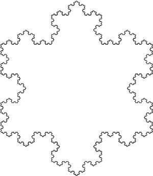
Figure 1. The Koch snowflake

Example 2.3.

Let $\Omega\subset{\mathbb{R}}^{2}$ be the Koch snowflake (see Figure 1) and let $\sigma:=\mathcal{H}^{1}|_{\partial\Omega}$. Then $\Gamma_{\sigma}^{\infty}=\partial\Omega$ so that $\Gamma_{\sigma}=D(\sigma)=\emptyset$. It is well-known that $\partial\Omega$ has Hausdorff dimension equal to $d:=\ln(4)/\ln(3),$ see [55]. In this case, the $d$-dimensional Hausdorff measure of $\partial\Omega$ is finite, $\mathcal{H}^{d}(\partial\Omega)<\infty,$ so that $\Gamma_{\mathcal{H}^{d}}^{\infty}=\emptyset$ and $D(\mathcal{H}^{d})=\Gamma_{\mathcal{H}^{d}}=\partial\Omega$.

Next, we give another example which is also meaningful for the applications.

Example 2.4.

Let now $\Omega\subset\mathbb{R}^{2}$ be the class of tree-shaped domains with self-similar fractal boundary introduced in [45]. Such a geometry can be seen as a two-dimensional idealization of the bronchial tree (see [1]; cf. also [2, 3, 4, 6]). In order to describe this set, we follow [1]. Consider four real numbers $a,\alpha,\beta,\theta$ such that $0<a<1/\sqrt{2}\emph{,}$ $\alpha>0$, $\beta>0$ and $0<\theta<\pi/2$. Let $f_{i},i=1,2,$ be two similitudes in $\mathbb{R}^{2}$ given by

$$f_{1}\left(x_{1},x_{2}\right) =\left(-\alpha,\beta\right)+a\left(x_{1}\cos\theta-x_{2}\sin\theta,x_{1}\sin\theta+x_{2}\cos\theta\right),$$

$$f_{2}\left(x_{1},x_{2}\right) =\left(\alpha,\beta\right)+a\left(x_{1}\cos\theta+x_{2}\sin\theta,-x_{1}\sin\theta+x_{2}\cos\theta\right).$$

One can define by $\Gamma_{f}$ the self-similar set associated to the similitudes $f_{1},f_{2}$, i.e., the unique compact subset of $\mathbb{R}^{2}$ such that $\Gamma_{f}=f_{1}\left(\Gamma_{f}\right)\cup f_{2}\left(\Gamma_{f}\right)$. To construct the ramified domain whose boundary is $\Gamma_{f}$, we further let $\mathbb{A}_{n}$ be the set containing all the $2^{n}$ mappings from $\{1,...,n\}$ to $\{1,2\},$ called strings of length $n$ for $n>1$, and define $\mathbb{A}=\bigcup\limits_{n\geq 1}\mathbb{A}_{n}$ as the set containing the empty string and all the finite strings. Next, consider two points $P_{1}=\left(-1,0\right)$ and $P_{2}=\left(1,0\right)$ and let $\Gamma_{b}$ be the line segment $\left[P_{1},P_{2}\right]$. We impose that $f_{2}\left(P_{1}\right)$ and $f_{2}\left(P_{2}\right)$ have positive coordinates (i.e., $a\cos\theta<\alpha$ and $a\sin\theta<\beta$). The first cell $Y_{0}$ of the tree domain $\Omega$ (i.e., the bottom of the tree, see Figure 2) is constructed by assuming that $Y_{0}$ is the convex, hexagonal, open domain inside the closed polygonal line joining the points $P_{1},$ $P_{2}$, $f_{2}\left(P_{2}\right)$, $f_{2}\left(P_{1}\right)$, $f_{1}\left(P_{2}\right)$, $f_{1}\left(P_{1}\right)$, and $P_{1}$ in this order. With the above assumptions on $\theta$,$\alpha,\beta,a,$ this is true if and only if $\left(\alpha-1\right)\sin\theta+\beta\cos\theta>0$. Under these assumptions, the domain $Y_{0}$ is contained in the half-plane $x_{2}>0$ and is symmetric with respect to the vertical axis $x_{1}=0$. Next, we introduce $K_{0}=\overline{Y_{0}}$. It is possible to glue together $K_{0}$, $f_{1}\left(K_{0}\right)$ and $f_{2}\left(K_{0}\right)$ and obtain a new polygonal domain, also symmetric with respect to the axis $x_{1}=0$. We define the ramified open domain $\Omega$,

$$\Omega=Interior\left(\bigcup\limits_{\sigma\in\mathbb{A}}f_{\sigma}\left(K_{0}\right)\right),$$

see Figure 2. Note that $\Omega$ is symmetric with respect to the axis $x_{1}=0$. In [45] it was proved that, for any $0<\theta<\pi/2,$ there exists a unique positive number $a_{\ast}<1/\sqrt{2},$ which does not depend on $\left(\alpha,\beta\right),$ such that for $0<a<a_{\ast}$, $\Gamma_{f}$ has ”no self-contact”. In this case the Hausdorff dimension of $\Gamma_{f}$ is $d=-\ln\left(2\right)/\ln\left(a\right)>1$ and by [5], $\Omega$ possesses the $W^{1,2}$-extension property of Sobolev functions. Moreover, since $\mathcal{H}^{d}(\Gamma_{f})<\infty$ we have $\Gamma_{\mathcal{H}^{d}}^{\infty}=\emptyset$ and $D(\mathcal{H}^{d})=\Gamma_{\mathcal{H}^{d}}=\partial\Omega\supset\Gamma_{f}$ (cf. Definition 2.1). On the other hand, note that for $\sigma=\mathcal{H}^{1}|_{\partial\Omega}$, we have $\Gamma_{\sigma}^{\infty}=\Gamma_{f}$ so that $\Gamma_{\sigma}=D(\sigma)=\partial\Omega\setminus\Gamma_{f}.$

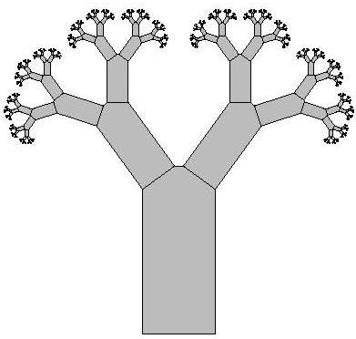
Figure 2. Tree-domain ($0<a<a_{\ast}$)

Definition 2.5.

Let $d\in[0,N]$ and let $\mu$ be a regular Borel measure on $\partial\Omega$.

1. We say that $\mu$ is an upper $d$-Ahlfors measure if there exists a constant $C_{2}>0$ such that for every $x\in\partial\Omega$ and every $r\in(0,1]$, one has

   $$\mu(B(x,r)\cap\partial\Omega)\leq C_{2}r^{d}.$$

2. We say that $\mu$ is a lower $d$-Ahlfors measure if there exists a constant $C_{1}>0$ such that for every $x\in\partial\Omega$ and every $r\in(0,1]$, one has

   $$\mu(B(x,r)\cap\partial\Omega)\geq C_{1}r^{d}.$$

By [13, Remark 2.20], every upper $d$-Ahlfors measure $\mu$ is absolutely continuous with respect to the $d$-dimensional Hausdorff measure $\mathcal{H}^{d}$, that is, there exists a function $f\in L^{\infty}(\partial\Omega,\mathcal{H}^{d})$ such that $\mu(A)=\int_{A}f\left(x\right)d\mathcal{H}^{d}$ for every Borel set $A\subset\partial\Omega$. Moreover, by [43, Lemma 1.17], the $d$-dimensional Hausdorff measure $\mathcal{H}^{d}$ is absolutely continuous with respect to every lower $d$-Ahlfors measure $\mu$.

Definition 2.6.

Let $F$ be a closed set in ${\mathbb{R}}^{N}$. We say that $F$ is a $d$-set for some $d\in(0,N]$ in the sense that there exist a Borel measure $\mu$ on $F$ and some constants $C_{2}>C_{1}>0$ such that

$$C_{1}r^{d}\leq\mu(F\cap B(x,r))\leq C_{2}r^{d}\;\text{ for all }x\in F\text{ and all }r\in(0,1],$$ (2.3)

where $B(x,r)$ is the Euclidean metric ball. Notice that a measure satisfying (2.3) is called a $d$-Ahlfors measure.

Let now $\Omega\subset\mathbb{R}^{N}$ be an arbitrary bounded domain with boundary $\partial\Omega.$ By [38] (see also [15]), $\partial\Omega$ is a $d$-set if and only if (2.3) holds with $\mu$ being the restriction to $\partial\Omega$ of the $d$-dimensional Hausdorff measure $\mathcal{H}^{d}$. Hence, it follows directly from (2.3) that $\mathcal{H}^{d}$ is an upper $d$-Ahlfors measure. In particular, $D(\mathcal{H}^{d})=\Gamma_{\mathcal{H}^{d}}=\partial\Omega$ so that $\Gamma_{\mathcal{H}^{d}}^{\infty}=\emptyset$. If $d>N-1$, then $D(\sigma)=\Gamma_{\sigma}=\emptyset$ so that $\Gamma_{\sigma}^{\infty}=\partial\Omega$, where we recall that $\sigma=\mathcal{H}^{N-1}|_{\partial\Omega}$.

Example 2.7.

Let $\Omega\subset\mathbb{R}^{2}$ be the Koch snowflake and recall that $d=\ln(4)/\ln(3)$ is the Hausdorff dimension of $\partial\Omega$ (cf. Example 2.3). By [55], the restriction of $\mathcal{H}^{d}$ to $\partial\Omega$ is an upper $d$-Ahlfors measure. Let now $\Omega\subset\mathbb{R}^{2}$ be the tree-domain in Example 2.4. By [37], there exists a unique regular Borel invariant measure $\mu$ on $\Gamma_{f}$ in the sense that for every Borel set $B,$ $\mu\left(B\right)=\mu\left(f_{1}^{-1}\left(B\right)\right)+\mu\left(f_{2}^{-1}\left(B\right)\right).$ The set $\Gamma_{f},$ endowed with the self-similar measure $\mu,$ is a d-set where $d=-\ln\left(2\right)/\ln\left(a\right)$ (see [1]), hence $\mu_{\mid\Gamma_{f}}=\mathcal{H}^{d}|_{\Gamma_{f}}$.

For more properties of Ahlfors measures and $d$-sets we refer the reader to [15, 21, 26, 38] and the references therein.

2.2. The Maz’ya space

In this subsection, we introduce the function spaces needed to study our problem. We recall that $\Omega\subset{\mathbb{R}}^{N}$ ($N\geq 2$) is an arbitrary bounded domain with boundary $\partial\Omega$ and the measure $\sigma=\mathcal{H}^{N-1}|_{\partial\Omega}$.

For $p\in[1,\infty)$, we denote by $W^{1,p}(\Omega)$ the first order Sobolev space endowed with the norm

$$\|u\|_{W^{1,p}(\Omega)}=\left(\|\nabla u\|_{p,\Omega}^{p}+\|u\|_{p,\Omega}^{p}\right)^{1/p}.$$

Then $W^{1,p}(\Omega)$ is a Banach space and $W^{1,2}(\Omega)$ is a Hilbert space. We let

$$\mathcal{W}^{1,2}(\Omega):=\overline{W^{1,2}(\Omega)\cap C(\overline{\Omega})}^{W^{1,2}(\Omega)}.$$

Then $\mathcal{W}^{1,2}(\Omega)$ is a proper closed subspace of $W^{1,2}(\Omega)$ such that they coincide if, for instance, $\Omega$ has the segment property (see [49, Theorem 1, p.28]). We recall that the latter property is equivalent to $\Omega$ being of class $C$, which is slightly weaker than the Lipschitz property of $\Omega.$

The following important inequality is due to Maz’ya [48, Section 3.6, p.189].

Theorem 2.8 (Maz’ya).

There is a constant $C=C(N)>0$ such that for every function $u\in W^{1,1}(\Omega)\cap C(\overline{\Omega})$,

$$\|u\|_{\frac{N}{N-1},\Omega}\leq C(N)\left(\|\nabla u\|_{1,\Omega}+\|u\|_{L^{1}(\partial\Omega,\sigma)}\right).$$ (2.4)

In the inequality (2.4), the constant $C(N)$ is exactly the so called isoperimetric constant.

The following result is a direct consequence of the Maz’ya inequality (2.4).

Corollary 2.9.

([49, Corollary 2.11.2]) Let $1\leq p<\infty$ and $p^{\star}:=pN/(N-1)$. There is a constant $C=C(N,p,\Omega)>0$ such that for every $u\in W^{1,p}(\Omega)\cap C(\overline{\Omega})$,

$$\|u\|_{p^{\star},\Omega}^{p}\leq C\left(\|\nabla u\|_{p,\Omega}^{p}+\|u\|_{L^{p}(\partial\Omega,\sigma)}^{p}\right).$$ (2.5)

Remark 2.10.

The exponent $p^{\star}$ in (2.5) is optimal in the sense that it cannot be improved without further regularity assumptions on $\Omega,$ see [49, Example 2.11, p.123].

Now, we let the classical Maz’ya space $W_{p,p}^{1}(\Omega,\partial\Omega)$ to be the abstract completion of

$$W_{\sigma,p}:=\{u\in W^{1,p}(\Omega)\cap C(\overline{\Omega}):\;\int_{\partial\Omega}|u|^{p}d\sigma<\infty\}$$

with respect to the norm

$$\|u\|_{W_{p,p}^{1}(\Omega,\partial\Omega)}=\left(\|\nabla u\|_{p,\Omega}^{p}+\|u\|_{L^{p}(\partial\Omega,\sigma)}^{p}\right)^{1/p}.$$

By (2.5), it follows that

$$W_{p,p}^{1}(\Omega,\partial\Omega)\hookrightarrow L^{p^{\star}}(\Omega)\;\mbox{(only continuous embedding)}.$$ (2.6)

In this paper, we focus on the Hilbert space case $p=2$, that is, the space $W_{2,2}^{1}(\Omega,\partial\Omega)$.

Next, let $\mu$ be an arbitrary regular Borel measure on the boundary $\partial\Omega$. We define the Maz’ya type space $W_{2,2}^{1}(\Omega,\partial\Omega,\mu)$ to be the abstract completion of

$$W_{\mu,2}:=\{u\in W^{1,2}(\Omega)\cap C(\overline{\Omega}):\;\int_{\partial\Omega}|u|^{2}d\mu<\infty\}$$

with respect to the norm

$$\|u\|_{W_{2,2}^{1}(\Omega,\partial\Omega,\mu)}=\left(\|u\|_{W^{1,2}(\Omega)}^{2}+\int_{\partial\Omega}|u|^{2}\,d\mu\right)^{1/2}.$$

It follows from (2.5) that the spaces $W_{2,2}^{1}(\Omega,\partial\Omega,\sigma)$ and $W_{2,2}^{1}(\Omega,\partial\Omega)$ coincide with equivalent norms.

Now, for a measurable function $u$ on $\partial\Omega$ and $s\in(0,1)$, we let

$$\mathcal{N}_{s,\mu}(u):=\int\int_{\partial\Omega\times\partial\Omega}K_{s}(x,y)|u(x)-u(y)|^{2}d\mu_{x}d\mu_{y},\text{ }K_{s}(x,y):=\frac{1}{|x-y|^{N-1+2s}}.$$

We let the fractional order Sobolev-Besov type space

$${H}^{s}(\partial\Omega,\mu):=\{u\in L^{2}(\partial\Omega,\mu):\;\;\mathcal{N}_{s,\mu}(u)<\infty\}$$

be equipped with the norm

$$\|u\|_{{H}^{s}(\partial\Omega,\mu)}:=\left(\|u\|_{L^{2}(\partial\Omega,\mu)}^{2}+\mathcal{N}_{s,\mu}(u)\right)^{1/2}.$$

For further properties of the space ${H}^{s}(\partial\Omega,\mu)$ we refer the reader to [21] and the references therein. Let $({H}^{s}(\partial\Omega,\mu))^{\ast}$ denote the dual of the Hilbert space ${H}^{s}(\partial\Omega,\mu)$. We define on the boundary a (nonlocal) operator $\Theta_{\mu}:\;{H}^{s}(\partial\Omega,\mu)\rightarrow({H}^{s}(\partial\Omega,\mu))^{\ast}$ as follows: for $u,v\in{H}^{s}(\partial\Omega,\mu)$ we set

$$\langle\Theta_{\mu}(u),v\rangle:=\int\int_{\partial\Omega\times\partial\Omega}K_{s}(x,y)(u(x)-u(y))(v(x)-v(y))d\mu_{x}d\mu_{y},$$ (2.7)

where $\langle\cdot,\cdot\rangle$ denotes the duality between ${H}^{s}(\partial\Omega,\mu)$ and $({H}^{s}(\partial\Omega,\mu))^{\ast}$. With some further abuse of notation, from now on $\langle\cdot,\cdot\rangle$ denotes the duality between any Banach space $X$ and its dual $X^{\ast}.$

Now, we let $\mathcal{V}_{\Theta}^{1,2}(\Omega,\partial\Omega,\mu)$ be the abstract completion of

$$W_{\mu,\Theta}:=\{u\in W_{\mu,2}:\;\int\int_{\partial\Omega\times\partial\Omega}K_{s}(x,y)|u(x)-u(y)|^{2}d\mu_{x}d\mu_{y}<\infty\}$$

with respect to the norm

$$\|u\|_{\mathcal{V}_{\Theta}^{1,2}(\Omega,\partial\Omega,\mu)}:=\left(\|u\|_{W^{1,2}(\Omega)}^{2}+\int_{\partial\Omega}|u|^{2}d\mu+\int\int_{\partial\Omega\times\partial\Omega}K_{s}(x,y)|u(x)-u(y)|^{2}d\mu_{x}d\mu_{y}\right)^{1/2}.$$

It is clear that $\mathcal{V}_{\Theta}^{1,2}(\Omega,\partial\Omega,\mu)$ is continuously embedded into $W_{2,2}^{1}(\Omega,\partial\Omega,\mu)$ and if $\mu=\sigma$, then

$$\||u\||:=\left(\|\nabla u\|_{2,\Omega}^{2}+\int_{\partial\Omega}|u|^{2}d\sigma+\int\int_{\partial\Omega\times\partial\Omega}K_{s}(x,y)|u(x)-u(y)|^{2}d\sigma_{x}d\sigma_{y}\right)^{1/2}.$$

defines an equivalent norm on the space $\mathcal{V}_{\Theta}^{1,2}(\Omega,\partial\Omega,\sigma),$ and this space is continuously embedded into $W_{2,2}^{1}(\Omega,\partial\Omega)$. We notice that if $\Omega$ has Lipschitz boundary, then the spaces $W_{2,2}^{1}(\Omega,\partial\Omega)=W_{2,2}^{1}(\Omega,\partial\Omega,\sigma)=W^{1,2}(\Omega)$ with equivalent norms. Moreover, if the measure $\mu\equiv 0$, then we always have $W_{2,2}^{1}(\Omega,\partial\Omega,0)=\mathcal{V}_{\Theta}^{1,2}(\Omega,\partial\Omega,0)=\mathcal{W}^{1,2}(\Omega)$ with equivalent norms. On the other hand, for arbitrary domains or/and for arbitrary regular Borel measures, in order to have an explicit description of the Maz’ya type space $W_{2,2}^{1}(\Omega,\partial\Omega,\mu)$ and its subspace $\mathcal{V}_{\Theta}^{1,2}(\Omega,\partial\Omega,\mu)$, we need the following notion of capacity.

Definition 2.11.

The relative capacity $Cap_{2,\Omega}$ with respect to $\Omega$ is defined for sets $A\subset\overline{\Omega}$ by

$$Cap_{2,\Omega}(A):=\inf\left\{\|u\|_{W^{1,2}(\Omega)}^{2}\;:\;\begin{array}[]{l}u\in{\mathcal{W}}^{1,2}(\Omega),\;\exists\;O\subset{\mathbb{R}}^{N}\text{ open,}\\ A\subset O\text{ and }u\geq 1\text{ a.e. on }\Omega\cap O\end{array}\right\}.$$

• A set $P\subset\overline{\Omega}$ is called $Cap_{2,\Omega}$-polar if $Cap_{2,\Omega}(P)=0$.

• We say that a property holds $Cap_{2,\Omega}$-quasi everywhere (briefly q.e.) on a set $A\subset\overline{\Omega}$, if there exists a $Cap_{2,\Omega}$-polar set $P$ such that the property holds for all $x\in A\setminus P$.

• A function $u$ is called $Cap_{2,\Omega}$-quasi continuous on a set $A\subset\overline{\Omega}$ if for all $\varepsilon>0$ there exists an open set $O$ in the metric space $\overline{\Omega}$ such that $Cap_{2,\Omega}(O)\leq\varepsilon$ and $u$ restricted to $A\setminus O$ is continuous.

The relative capacity $Cap_{2,\Omega}$ has been introduced in [8] (see also [9, 56, 59] for a more general version) to study the Laplace operator with linear (local) Robin boundary conditions on arbitrary open subsets in ${\mathbb{R}}^{N}$. Note that if $\Omega={\mathbb{R}}^{N}$, then $Cap_{2,\mathbb{R}^{N}}=Cap_{2}$ is the classical Wiener capacity [11, 25]. By [8, Section 2], for every $u\in{\mathcal{W}}^{1,2}(\Omega)$ there exists a unique (up to a $Cap_{2,\Omega}$-polar set) $Cap_{2,\Omega}$-quasi continuous function $\tilde{u}:\overline{\Omega}\rightarrow{\mathbb{R}}$ such that $\tilde{u}=u$ a.e. on $\Omega$. Moreover, if $u\in{\mathcal{W}}^{1,2}(\Omega)$ and $u_{n}\in{\mathcal{W}}^{1,2}(\Omega)$ is a sequence which converges to $u$ in ${\mathcal{W}}^{1,2}(\Omega)$, then there is a subsequence of $\tilde{u}_{n}$ which converges to $\tilde{u}$ q.e. on $\overline{\Omega}$.

We have the following situation regarding the Maz’ya type space $W_{2,2}^{1}(\Omega,\partial\Omega,\mu)$. Let $\Gamma_{\mu}^{\infty}$ be the relatively closed, and let $D(\mu)=\Gamma_{\mu}$ be the relatively open subsets of $\partial\Omega$ defined in (2.1) and (2.2), respectively. Then every function $u\in W_{\mu,2}$ is such that $u|_{\Gamma_{\mu}^{\infty}}=0$, where we recall that

$$W_{\mu,2}:=\{u\in W^{1,2}(\Omega)\cap C(\overline{\Omega}):\;\int_{\partial\Omega}|u|^{2}d\mu<\infty\}.$$

Let $\Gamma\subset\partial\Omega$ be a relatively closed set. Since the closure of the set $\{u\in W^{1,2}(\Omega)\cap C(\overline{\Omega}):\;u|_{\Gamma}=0\}$ in $W^{1,2}(\Omega)$ is the space $\{u\in\mathcal{W}^{1,2}(\Omega):\;\tilde{u}=0\;\mbox{ q.e. on }\;\Gamma\}$, it follows that every function $u$ in $W_{2,2}^{1}(\Omega,\partial\Omega,\mu)$ is zero q.e. on $\Gamma_{\mu}^{\infty}$ (see [8, 9]). With these observations, one has the following descriptions:

$$W_{2,2}^{1}(\Omega,\partial\Omega,\mu)=\{u\in{\mathcal{W}}^{1,2}(\Omega),\;\tilde{u}=0\;\mbox{ q.e. on }\;\Gamma_{\mu}^{\infty}\;\mbox{ and }\int_{\Gamma_{\mu}}|\tilde{u}|^{2}d\mu<\infty\}$$ (2.8)

and

$$\mathcal{V}_{\Theta}^{1,2}(\Omega,\partial\Omega,\mu)=\{u\in W_{2,2}^{1}(\Omega,\partial\Omega,\mu),\;\;\int\int_{\Gamma_{\mu}\times\Gamma_{\mu}}K_{s}(x,y)|\tilde{u}(x)-\tilde{u}(y)|^{2}d\mu_{x}d\mu_{y}<\infty\}.$$ (2.9)

Note that if $\Gamma_{\mu}^{\infty}=\partial\Omega$ or $\mathop{\mathrm{C}ap}_{2,\Omega}(\Gamma_{\mu})=0$, then $W_{2,2}^{1}(\Omega,\partial\Omega,\mu)=\mathcal{V}_{\Theta}^{1,2}(\Omega,\partial\Omega,\mu)=W_{0}^{1,2}(\Omega):=\overline{\mathcal{D}(\Omega)}^{W^{1,2}(\Omega)}$. This is the case for the well-known $2$-dimensional open set bounded by the Koch snowflake if one takes the measure $\mu=\sigma$ and is also the case for $d$-sets if $\mu=\sigma$ and $d>N-1$.

Throughout the remainder, we identify each function $u\in{\mathcal{W}}^{1,2}(\Omega)$ with its quasi-continuous version $\tilde{u}$. With this identification, we define the bilinear symmetric form $\mathcal{A}_{\Theta,\mu}$ with domain $\mathcal{V}_{\Theta}^{1,2}(\Omega,\partial\Omega,\mu)$ by

$$\mathcal{A}_{\Theta,\mu}(u,v):= \int_{\Omega}\nabla u\cdot\nabla vdx+\int_{\partial\Omega}uvd\mu$$

$$+\int\int_{\partial\Omega\times\partial\Omega}K_{s}(x,y)(u(x)-u(y))(v(x)-v(y))d\mu_{x}d\mu_{y}.$$ (2.10)

Since every function $u\in\mathcal{V}_{\Theta}^{1,2}(\Omega,\partial\Omega,\mu)$ is such that $u=0$ q.e. on $\Gamma_{\mu}^{\infty}$, one has that the form $\mathcal{A}_{\Theta,\mu}$ defined in (2.10) is given by

$$\mathcal{A}_{\Theta,\mu}(u,v):= \int_{\Omega}\nabla u\cdot\nabla vdx+\int_{\Gamma_{\mu}}uvd\mu$$

$$+\int\int_{\Gamma_{\mu}\times\Gamma_{\mu}}K_{s}(x,y)(u(x)-u(y))(v(x)-v(y))d\mu_{x}d\mu_{y}.$$ (2.11)

The form $\mathcal{A}_{\Theta,\mu}$ is closed on $L^{2}(\Omega)$ if and only if the functional $\varphi_{\Theta,\mu}:\;L^{2}(\Omega)\rightarrow[0,+\infty]$ defined by

$$\varphi_{\Theta,\mu}(u):=\begin{cases}\frac{1}{2}\mathcal{A}_{\Theta,\mu}(u,u)\;\;\;&\mbox{ if }\;u\in\mathcal{V}_{\Theta}^{1,2}(\Omega,\partial\Omega,\mu),\\ +\infty&\mbox{ if }\;u\in L^{2}(\Omega)\setminus\mathcal{V}_{\Theta}^{1,2}(\Omega,\partial\Omega,\mu)\end{cases}$$

is lower semi-continuous on $L^{2}(\Omega)$. To characterize the lower semi-continuity of $\varphi_{\Theta,\mu}$, and hence, the closedness of $\mathcal{A}_{\Theta,\mu}$, we need to following notion of boundary regularity and/or measure regularity.

Definition 2.12.

We say that a subset $\Gamma$ of $\partial\Omega$ is $\mathop{\mathrm{C}ap}_{2,\Omega}$-admissible with respect to $\mu$, if for every Borel set $A\subset\Gamma$, one has $\mathop{\mathrm{C}ap}_{2,\Omega}(A)=0$ implies $\mu(A)=0$.

The following result is taken from [59, Theorems 4.4 and 5.2] (see also [56, Theorem 4.2.1] and [13, Theorem 2.11]).

Theorem 2.13.

The following assertions are equivalent.

1. The operator $R:\;W_{2,2}^{1}(\Omega,\partial\Omega,\mu)\rightarrow L^{2}(\Omega)$, $u\mapsto u|_{\Omega}$ is injective.

2. The set $\Gamma_{\mu}$ is $\mathop{\mathrm{C}ap}_{2,\Omega}$-admissible with respect to $\mu$.

3. The bilinear form $\mathcal{A}_{\Theta,\mu}$ is closed on $L^{2}(\Omega)$.

To see that Theorem 2.13 applies to a large class of rough domains, let us recall that $\Omega$ is said to have the $W^{1,2}$-extension property if for every $u\in W^{1,2}(\Omega)$ there exists $U\in W^{1,2}({\mathbb{R}}^{N})$ such that $U|_{\Omega}=u$ a.e. In that case, by [34, Theorem 5], there exists a bounded linear extension operator $\mathcal{E}$ from $W^{1,2}(\Omega)$ into $W^{1,2}({\mathbb{R}}^{N})$. It is worth emphasizing that for extension domains the spaces $\mathcal{W}^{1,2}(\Omega)$ and $W^{1,2}(\Omega)$ coincide. The following important result is proven in [59, Lemma 4.7].

Theorem 2.14.

If $\Omega\subset{\mathbb{R}}^{N}$ ($N\geq 2$) has the $W^{1,2}$-extension property, then $\partial\Omega$ is $\mathop{\mathrm{C}ap}_{2,\Omega}$-admissible with respect to $\mu=\mathcal{H}_{\mid\partial\Omega}^{d},$ the $d$-dimensional Hausdorff measure of $\partial\Omega,$ for any $d\in(N-2,N).$

Furthermore, if $\mu$ is an upper $d$ -Ahlfors measure on $\partial\Omega$ for some $d\in(N-2,N)\cap(0,N)$, then by [13, Remark 2.20], $\partial\Omega$ is $\mathop{\mathrm{C}ap}_{2,\Omega}$-admissible with respect to $\mu$. In particular, since bounded Lipschitz domains and, for example, the Koch snowflake and the ramified tree domains (see Examples 2.3 and 2.4, respectively), have the $W^{1,2}$-extension property then their boundaries are $\mathop{\mathrm{C}ap}_{2,\Omega}$-admissible with respect to $\sigma$. For the Koch snowflake and the tree domain, $\partial\Omega$ is also $\mathop{\mathrm{C}ap}_{2,\Omega}$-admissible with respect to $\mathcal{H}_{\mid\partial\Omega}^{d}$ where $d=\ln(4)/\ln(3)$ for the snowflake and $d=-\ln(2)/\ln(a)$ for the tree domain, respectively. Some examples of open sets, whose boundaries are not $\mathop{\mathrm{C}ap}_{2,\Omega}$-admissible with respect to $\sigma$ are contained in [8, Examples 1.5, 1.6, 4.2, 4.3].

2.3. The Laplacian with nonlocal Robin boundary conditions

In this subsection we define a realization of the Laplace operator with nonlocal Robin boundary conditions on $L^{2}(\Omega)$. We also deduce some properties of this operator that are needed to prove our main results.

Throughout the remainder of this article, we assume that $\Omega\subset{\mathbb{R}}^{N}$ is a bounded domain with boundary $\partial\Omega$, $\mu$ is a regular Borel measure on $\partial\Omega$ such that its domain $\Gamma_{\mu}$ defined in (2.2) is $\mathop{\mathrm{C}ap}_{2,\Omega}$-admissible with respect to $\mu$. Then, by Theorem 2.13, the bilinear form $\mathcal{A}_{\Theta,\mu}$ defined in (2.11) is closed on $L^{2}(\Omega)$. Let $A_{\Theta,\mu}$ be the closed, linear, self-adjoint operator associated with $\mathcal{A}_{\Theta,\mu}$ in the sense that

$$\begin{cases}D(A_{\Theta,\mu})&:=\{u\in\mathcal{V}_{\Theta}^{1,2}(\Omega,\partial\Omega,\mu),\;\exists\;v\in L^{2}(\Omega),\;\mathcal{A}_{\Theta,\mu}(u,\varphi)=(v,\varphi)_{L^{2}(\Omega)},\;\forall\;\varphi\in\mathcal{V}_{\Theta}^{1,2}(\Omega,\partial\Omega,\mu)\}\\ A_{\Theta,\mu}u&:=v.\end{cases}$$ (2.12)

The operator $A_{\Theta,\mu}$ can be described explicitly as follows:

$$D(A_{\Theta,\mu})=\{u\in\mathcal{V}_{\Theta}^{1,2}(\Omega,\partial\Omega,\mu):\Delta u\in L^{2}(\Omega),\;\partial_{\nu}ud\sigma+(u+\Theta_{\mu}(u))d\mu=0\;\mbox{ on }\;\partial\Omega\},$$

and

$$A_{\Theta,\mu}u=-\Delta u.$$

We note that if $\mu=\sigma$ or, more generally, if $\mu$ is absolutely continuous with respect to $\sigma$ (in particular, $d\mu_{x}=b\left(x\right)d\sigma_{x}$, for some nonnegative bounded measurable function $b\left(x\right)\in L^{\infty}\left(\partial\Omega\right)$), then

$$D(A_{\Theta,\sigma})=\{u\in\mathcal{V}_{\Theta}^{1,2}(\Omega,\partial\Omega,\sigma):\Delta u\in L^{2}(\Omega),\;\partial_{\nu}u+b(x)u+a(x,y)\Theta_{\sigma}(u)=0\;\mbox{ on }\;\partial\Omega\},$$

which corresponds to the classical (or usual) nonlocal Robin boundary conditions. Here $a\left(x,y\right)=b\left(x\right)b\left(y\right)$ is a bounded measurable function on $\partial\Omega\times\partial\Omega$ such that $d\mu_{x}d\mu_{y}=a\left(x,y\right)d\sigma_{x}d\sigma_{y}$. We also notice that the description (2.9) for $\mathcal{V}_{\Theta}^{1,2}(\Omega,\partial\Omega,\mu)$ shows that one always has a Dirichlet boundary conditions on the part $\Gamma_{\mu}^{\infty}$. Clearly the operator $A_{\Theta,\mu},$ defined above, satisfies

$$A_{\Theta,\mu}:\;\mathcal{V}_{\Theta}^{1,2}(\Omega,\partial\Omega,\mu)\rightarrow(\mathcal{V}_{\Theta}^{1,2}(\Omega,\partial\Omega,\mu))^{\ast},$$ (2.13)

that is, $A_{\Theta,\mu}$ maps $\mathcal{V}_{\Theta}^{1,2}(\Omega,\partial\Omega,\mu)$ into $(\mathcal{V}_{\Theta}^{1,2}(\Omega,\partial\Omega,\mu))^{\ast}$.

Throughout the remainder of this article, if $\mu$ is absolutely continuous with respect to $\sigma$, we will simply say that $\mu=\sigma$. We have the following result.

Theorem 2.15.

Let $\Gamma_{\mu}$ be $\mathop{\mathrm{C}ap}_{2,\Omega}$-admissible with respect to $\mu$. Assume that either $\mu=\sigma$ or that

$$\mathcal{V}_{\Theta}^{1,2}(\Omega,\partial\Omega,\mu)\hookrightarrow L^{2q}(\Omega)\mbox{ for some }q=q\left(N,\Omega\right)>1\;\mbox{ if }\;\mu\neq\sigma.$$ (2.14)

Then the following assertions hold.

1. The operator $-A_{\Theta,\mu}$ generates a strongly continuous semigroup $(e^{-tA_{\Theta,\mu}})_{t\geq 0}$ of contractions on $L^{2}(\Omega)$ which can be extended to contraction strongly continuous semigroups on $L^{p}(\Omega)$ for every $p\in[1,\infty)$.

2. The operator $A_{\Theta,\mu}$ has a compact resolvent, and hence has a discrete spectrum. The spectrum of $A_{\Theta,\mu}$ is an increasing sequence of real numbers $0\leq\lambda_{1}<\lambda_{2}<\cdots<\lambda_{n}<\dots,$ that converges to $+\infty$. Moreover, if $u_{n}$ is an eigenfunction associated with $\lambda_{n}$, then $u_{n}\in D\left(A_{\Theta,\mu}\right)\cap L^{\infty}(\Omega)$.

3. Assume also that either $\mathop{\mathrm{C}ap}_{2,\Omega}(\Gamma_{\mu}^{\infty})>0$ or $\mu(\Gamma_{\mu})>0$. Then $0\in\rho(A_{\Theta,\mu}),$ the resolvent set of $A_{\Theta,\mu}$, and there exists a constant $C>0$ such that, for every $u\in\mathcal{V}_{\Theta}^{1,2}(\Omega,\partial\Omega,\mu)$,

   $$\|u\|_{2,\Omega}^{2}\leq C\mathcal{A}_{\Theta,\mu}(u,u).$$ (2.15)

4. Denoting the generator of the semigroup on $L^{p}(\Omega)$ by $A_{p,\Theta,\mu}$, so that $A_{\Theta,\mu}=A_{2,\Theta,\mu}$, then the spectrum of $A_{p,\Theta,\mu}$ is independent of $p$. The spectral bound

   $$s\left(A_{p,\Theta,\mu}\right)=\inf\left\{\mathop{\mathrm{R}e}\lambda:\lambda\in\sigma\left(A_{p,\Theta,\mu}\right)\right\}$$

   of $A_{p,\Theta,\mu}$ is an algebraically simple eigenvalue. It is the only eigenvalue having a positive eigenfunction.

5. For each $\theta\in(0,1]$, there holds $D(A_{\Theta,\mu}^{\theta})\subset L^{\infty}\left(\Omega\right)$ provided that $\theta>\gamma.$ Here, $\gamma=N/2$ if $\mu=\sigma$ and $\gamma=q/2(q-1)$ if $\mu\neq\sigma$.

Proof.

(a) This part follows from [59, Corollary 5.3] (where the assumption (2.14) is not needed).

(b) First, we notice that since we have assumed that $\Gamma_{\mu}$ is $\mathop{\mathrm{C}ap}_{2,\Omega}$-admissible with respect to $\mu$, we have from Theorem 2.13 that the continuous embedding $\mathcal{V}_{\Theta}^{1,2}(\Omega,\partial\Omega,\mu)\hookrightarrow L^{2}(\Omega)$ is also an injection. Moreover it follows from (2.6) if $\mu=\sigma$ and the assumption (2.14) if $\mu\neq\sigma$, that the embedding $\mathcal{V}_{\Theta}^{1,2}(\Omega,\partial\Omega,\mu)\hookrightarrow L^{2}(\Omega)$ is compact since $\Omega$ is bounded. Since $A_{\Theta,\mu}$ is a nonnegative self-adjoint operator and has a compact resolvent, then it has a discrete spectrum which is an increasing sequence of real numbers $0\leq\lambda_{1}<\lambda_{2}<\cdots<\lambda_{n}\dots,$ that converges to $+\infty$.

Now, let $u_{n}\in\mathcal{V}_{\Theta}^{1,2}(\Omega,\partial\Omega,\mu)$ be an eigenfunction associated with $\lambda_{n}$. Then, for every $v\in\mathcal{V}_{\Theta}^{1,2}(\Omega,\partial\Omega,\mu)$,

$$\int_{\Omega}\nabla u_{n}\cdot\nabla vdx+\int_{\Gamma_{\mu}}u_{n}vd\mu$$

$$+\int\int_{\Gamma_{\mu}\times\Gamma_{\mu}}K_{s}\left(x,y\right)(u_{n}(x)-u_{n}(y))(v(x)-v(y))d\mu_{x}d\mu_{y}=\lambda_{n}\int_{\Omega}u_{n}vdx.$$

This equality means that $A_{\Theta,\mu}u_{n}=\lambda_{n}u_{n}$. Let $\alpha>0$ be a real number. Since $\alpha\in\rho(-A_{\Theta,\mu})$, we have that $\alpha I+A_{\Theta,\mu}$ is invertible. From $A_{\Theta,\mu}u_{n}=\lambda_{n}u_{n}$ we have that

$$u_{n}=(\alpha I+A_{\Theta,\mu})^{-1}(\lambda_{n}+\alpha)u_{n}=(\lambda_{n}+\alpha)(\alpha I+A_{\Theta,\mu})^{-1}(u_{n}).$$

By [59, Theorem 5.4], the semigroup $(e^{-tA_{\Theta,\mu}})_{t\geq 0}$ is ultracontrative in the sense that it maps $L^{2}(\Omega)$ into $L^{\infty}(\Omega)$ (this follows from (2.6) if $\mu=\sigma,$ and from the assumption (2.14) if $\mu\neq\sigma$). More precisely, there is a constant $C>0$ and $\gamma\in(0,1)$ such that for every $f\in L^{2}(\Omega)$ and $t\in(0,1)$,

$$\|e^{-tA_{\Theta,\mu}}f\|_{\infty,\Omega}\leq Ct^{-\gamma}\left\|f\right\|_{2,\Omega}$$ (2.16)

where $\gamma=N/2$ if $\mu=\sigma$ and $\gamma=q/2(q-1)$ if $\mu\neq\sigma$. Since for every $f\in L^{2}(\Omega)$ and $\alpha>0$,

$$(\alpha I+A_{\Theta,\mu})^{-1}f=\int_{0}^{\infty}e^{-\alpha t}e^{-tA_{\Theta,\mu}}fdt,$$

it follows from (2.16) that there exists a constant $M>0$ such that

$$\|u_{n}\|_{\infty,\Omega}\leq M(\lambda_{n}+\alpha)\|u_{n}\|_{2,\Omega}.$$

This completes the proof of part (b).

(c) Assume to the contrary that $0\notin\rho(A_{\Theta,\mu})$ (i.e., $0$ is an eigenvalue for $A_{\Theta,\mu}$). Then there exists a nonzero function $u\in D(A_{\Theta,\mu})$ such that $A_{\Theta,\mu}u=0$, that is, $\mathcal{A}_{\Theta,\mu}(u,v)=0,$ for every $v\in\mathcal{V}_{\Theta}^{1,2}(\Omega,\partial\Omega,\mu)$. In particular, we have

$$\mathcal{A}_{\Theta,\mu}(u,u):=\int_{\Omega}|\nabla u|^{2}dx+\int_{\Gamma_{\mu}}|u|^{2}d\mu+\int\int_{\Gamma_{\mu}\times\Gamma_{\mu}}K_{s}(x,y)|u(x)-u(y)|^{2}d\mu_{x}d\mu_{y}=0.$$

This shows that $|\nabla u|=0$. Since $\Omega$ is bounded and connected, we get that $u=C_{1}$ for some constant $C_{1}$. Since $u=0$ q.e. on $\Gamma_{\mu}^{\infty}$ (as $u$ belongs to $\mathcal{V}_{\Theta}^{1,2}(\Omega,\partial\Omega,\mu)$), there are two alternatives. First, $\mathop{\mathrm{C}ap}_{2,\Omega}(\Gamma_{\mu}^{\infty})>0$ in which case $u=C_{1}\not\in D(A_{\Theta,\mu})$, whence a contradiction. On the other hand, from the facts that $u=C_{1}$, we get from the previous equation that $C_{1}\mu(\Gamma_{\mu})=0$. The second alternative $\mu(\Gamma_{\mu})>0$ then implies that $u=C_{1}=0$, again a contradiction. We have shown that $0\in\rho(A_{\Theta,\mu})$. Now the estimate (2.15) follows from standard properties of semigroups (see, e.g., [23, 30]), since we have just shown that there exists a constant $w>0$ such that $\|e^{-tA_{\Theta,\mu}}\|_{\mathcal{L}(L^{2}(\Omega),L^{2}(\Omega))}\leq e^{-wt}$ for every $t>0$ . This completes the proof of part (c).

(d) Let $A_{p,\Theta,\mu}$ be the generator of the semigroup on $L^{p}(\Omega)$. Since $A_{\Theta,\mu}=A_{2,\Theta,\mu}$ has a compact resolvent and $\Omega$ is bounded, it follows from the ultracontractivity that each semigroup has a compact resolvent on $L^{p}(\Omega)$ for $p\in[1,\infty]$. Now it follows from [23, Corollary 1.6.2] that the spectrum of $A_{p,\Theta,\mu}$ is independent of $p$. The last assertion in (d) follows from [18, Proposition 5.9 and Corollary 5.10].

(e) Since $I+A_{\Theta,\mu}$ is invertible we have that the $L^{2}\left(\Omega\right)$-norm of $\left(I+A_{\Theta,\mu}\right)^{\theta}$ defines an equivalent norm on $D(A_{\Theta,\mu}^{\theta})$ and

$$\left(I+A_{\Theta,\mu}\right)^{-\theta}=\frac{1}{\Gamma\left(\theta\right)}\int_{0}^{\infty}t^{\theta-1}e^{-t}e^{-tA_{\Theta,\mu}}fdt.$$

Using (2.16) for $t\in\left(0,1\right)$ and the contractivity of $e^{-tA_{\Theta,\mu}}$ for $t>1$, for $u\in D(A_{\Theta,\mu}^{\theta})$, we deduce

$$\left\|u\right\|_{L^{\infty}\left(\Omega\right)}\leq C\left\|u\right\|_{D(A_{\Theta,\mu}^{\theta})}\int_{0}^{1}t^{\theta-1-\gamma}dt+C\left\|u\right\|_{D(A_{\Theta,\mu}^{\theta})}\int_{1}^{\infty}e^{-t}dt.$$

The first integral is finite if and only if $\gamma<\theta$. The proof of theorem is finished.    

Remark 2.16.

1. We remark that either $\mathop{\mathrm{C}ap}_{2,\Omega}(\Gamma_{\mu}^{\infty})>0$ or $\mu(\Gamma_{\mu})>0,$ in part (c) of Theorem 2.15, is actually not an assumption about the regularity of the open set $\Omega$, but it is only an assumption about the measure $\mu$. Roughly speaking, it means that the trivial choice $\mu\equiv 0$ (the zero measure) is not allowed.

2. In the case of domains with Lipschitz continuous boundary $\partial\Omega,$ further interesting spectral properties for the operator $A_{\Theta,\mu}$ can be also derived (see [33]).

3. Assuming that either $\mathop{\mathrm{C}ap}_{2,\Omega}(\Gamma_{\mu}^{\infty})>0$ or $\mu(\Gamma_{\mu})>0$ is satisfied, we deduce from (2.15),

   $$\||u\||_{\mathcal{V}_{\Theta}^{1,2}(\Omega,\partial\Omega,\mu)}:=\left(\|\nabla u\|_{2,\Omega}^{2}+\|u\|_{L^{2}(\Gamma_{\mu})}^{2}+\mathcal{N}_{s,\mu}(u)\right)^{1/2}$$ (2.17)

   defines an equivalent norm on the space $\mathcal{V}_{\Theta}^{1,2}(\Omega,\partial\Omega,\mu)$. In particular, under the same assumption, we also have that

   $$\||u\||_{W_{2,2}^{1}(\Omega,\partial\Omega,\mu)}:=\left(\|\nabla u\|_{2,\Omega}^{2}+\|u\|_{L^{2}(\Gamma_{\mu})}^{2}\right)^{1/2}$$ (2.18)

   defines an equivalent norm on the space $W_{2,2}^{1}(\Omega,\partial\Omega,\mu)$.

4. In the case when $\theta\in(0,1]$ and $\mu=\sigma$, the embedding $D(A_{\Theta,\mu}^{\theta})\subset L^{\infty}\left(\Omega\right)$ holds provided that $N<2\theta$. This consideration is optimal for an arbitrary open subset $\Omega\subset R^{N}$ in view of Remark 2.10. Finally, when $\Omega$ has the $W^{1,2}$-extension property of Sobolev functions, we have $q=N/\left(N-2\right)$ for $N\geq 3$ and $q\in\left(1,\infty\right)$ for $N=2$. In that case $D(A_{\Theta,\mu}^{\theta})\subset L^{\infty}\left(\Omega\right)$ provided that $N<4\theta$ if $N\geq 3$. In a smooth situation (say when $\partial\Omega\in\mathcal{C}^{2}$), one has $D(A_{\Theta,\mu})\subset W^{2,2}\left(\Omega\right)$ and thus $D(A_{\Theta,\mu}^{\theta})\subset W^{2\theta,2}\left(\Omega\right)$. It is well-known that the embedding $W^{2\theta,2}\left(\Omega\right)\subset L^{\infty}\left(\Omega\right)$ holds in the smooth setting provided that $N<4\theta.$ This shows that the stated embedding $D(A_{\Theta,\mu}^{\theta})\subset L^{\infty}\left(\Omega\right)$ appears to be optimal in the non-smooth setting in this sense.

It is important to observe that the operator $A_{\Theta,\mu}$ depends on the choice of the measure $\mu$ on $\partial\Omega.$ In order to see this, consider Example 2.3 when $\Omega$ is the Koch snowflake in $\mathbb{R}^{2}$ and take $\mu=\sigma=\mathcal{H}_{\mid\partial\Omega}^{1}$. For this choice, $\sigma$ is locally infinite on $\partial\Omega$ so that there are no Robin boundary conditions for $\Omega$, on account of the description (2.8)-(2.9). Indeed, we have [8, Theorem 2.3],

$$D\left(\mathcal{A}_{\Theta,\sigma}\right)=\left\{u\in\mathcal{W}^{1,2}\left(\Omega\right):u=0\text{ q.e. on }\partial\Omega\right\}=W_{0}^{1,2}\left(\Omega\right)$$

and, consequently, $A_{\Theta,\sigma}$ coincides with the realization of the Laplace operator $-\Delta$ with homogeneous Dirichlet boundary conditions on $\partial\Omega$. However, with a different choice $\mu=\mathcal{H}_{\mid\partial\Omega}^{d}$ (where $d=\ln\left(4\right)/\ln\left(3\right)$ is the Hausdorff dimension of $\partial\Omega$), we have the generalized Robin boundary condition (1.2) on $\partial\Omega$ since $\Gamma_{\mu}^{\infty}=\emptyset$ (see Example 2.3). This is also the case for the tree-domain $\Omega$ of Example 2.4, in which case $A_{\Theta,\sigma}$ coincides exactly with the realization of the Laplace operator with homogeneous Dirichlet boundary conditions on $\Gamma_{f}$ (the small structures), and nonlocal Robin boundary conditions on $\partial\Omega\setminus\Gamma_{f}$. However, recall that the fractal boundary $\Gamma_{f}$ of $\Omega$ is a $d$-set, with $d=-\ln\left(2\right)/\ln\left(a\right).$ Thus, the natural measure $\mu$ of $\partial\Omega$ should be once again the $d$-dimensional Hausdorff measure $\mu=\mathcal{H}_{\mid\partial\Omega}^{d}$ so that the generalized (nonlocal) Robin boundary condition (1.2) is still realized on the portion $\Gamma_{f}$. In fact, a more appropriate choice for $\mu$ is

$$\mu=\left\{\begin{array}[]{ll}\mathcal{H}^{d},&\text{on }\Gamma_{f},\\ \sigma,&\text{on }\partial\Omega\setminus\Gamma_{f},\end{array}\right.$$

so that one has the usual (nonlocal) Robin boundary conditions on the portion $\partial\Omega\setminus\Gamma_{f},$ and the generalized (nonlocal) Robin boundary conditions on $\Gamma_{f}$. In the general case when $\Omega\subset\mathbb{R}^{N}$, such arguments also hold if $\partial\Omega$ is a $d$-set with $d\in(N-1,N].$

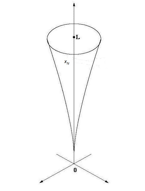
Figure 3. Cusp-shaped domain

Finally, it is worth emphasizing that the assumption (2.14) in Theorem 2.15 is satisfied with $q=N/(N-2)$ if, for example, $\Omega$ has the $W^{1,2}$-extension property. On the other hand, if $\Omega\subset{\mathbb{R}}^{N}$ is a non-Lipschitz bounded domain whose boundary admits a finite numbers of outward or inward Hölder cusps points and exponent at cusp points $0<\gamma<1$, then $\Omega$ does not enjoy the extension property. However, for such domains $\Omega$ we still have the following continuous embeddings:

$$\mathcal{V}_{\Theta}^{1,2}(\Omega,\partial\Omega,\mu)\hookrightarrow W^{1,2}(\Omega)\hookrightarrow L^{2q}(\Omega)\;\mbox{ with }\;q:=\frac{(N-1+\gamma)}{N-1-\gamma}>1,$$ (2.19)

see [28, 29]. Many examples of domains with cusps, which are the simplest non-Lipschitz domains used in the applications, can be found in [49, Chapters 7-8]; see, for instance, Example 2.17 below. For Hölder $C^{\gamma}$-domains and for the measure $\mu=\sigma=\mathcal{H}_{\mid\partial\Omega}^{N-1},$ we have from Definition 2.1 that $\Gamma_{\sigma}^{\infty}=\emptyset$, whereas $\Gamma_{\sigma}=D\left(\sigma\right)=\partial\Omega$. Thus, it is clear that in such cases, the usual (nonlocal) Robin boundary condition (1.2) is satisfied on $\Gamma_{\sigma}=\partial\Omega.$

Example 2.17.

(see Figure 3) Let $\Omega_{hc}\subset\mathbb{R}^{N}$, $N\geq 2$ be the following set:

$$\Omega_{hc}:=\left\{x=\left(x_{1},x_{2},...,x_{N}\right)\in\mathbb{R}^{N}:x_{N}\in\left(0,L\right),0<\sum\nolimits_{j=1}^{N-1}x_{i}^{2}<lx_{N}^{2/\gamma}\right\},$$

for some $L,l>0$ and $\gamma\in\left(0,1\right)$. The inequality (2.19) is fulfilled for $\Omega=\Omega_{hc}$ and $N\geq 2$. Generally, the Sobolev inequality (2.19) is satisfied in any Hölder domain $\Omega$ of class $C^{\gamma}$, $\gamma\in\left(0,1\right)$. By a (bounded) Hölder $C^{\gamma}$-domain we mean the following: there exist a finite number of balls $B\left(x_{i},r_{i}\right)$, $i=1,...,m_{N}$, whose union contains $\Omega$, and for each $i=1,...,m_{N}$, there exists a Hölder-continuous ($C^{\gamma},$ $\gamma\in\left(0,1\right)$) function $F_{i}:\mathbb{R}^{N-1}\rightarrow\mathbb{R}$ such that for some coordinate system, $B\left(x_{i},r_{i}\right)\cap\Omega$ is equal to the intersection of $B\left(x_{i},r_{i}\right)$ with the region above the graph of $F_{i}$.

3. Well-posedness and regularity

In this section $\Omega\subset{\mathbb{R}}^{N}$ is an arbitrary bounded domain with boundary $\partial\Omega$, $\mu$ is a regular Borel measure on $\partial\Omega$ such that $\mu$ is either the $\left(N-1\right)$-dimensional Hausdorff meausure $\mathcal{H}_{\mid\partial\Omega}^{N-1}$ or another ”arbitrary” regular Borel measure, according to the assumptions of Section 2 (see (H_μ) below). We begin this section by stating all the hypotheses on $f$ we need, even though not all of them must be satisfied at the same time.

1. $f\in C_{\text{loc}}^{1}\left(\mathbb{R}\right)$ satisfies

   $$\liminf_{\left|s\right|\rightarrow+\infty}\frac{f\left(s\right)}{s}>-\lambda_{\ast},$$

   for some constant $\lambda_{\ast}\in[0,C_{\Omega})$, where $C_{\Omega}=C\left(N,\Omega\right)>0$ is the best Sobolev/Poincaré constant into (2.5) and (2.14), respectively.

2. $f\in C_{\text{loc}}^{1}\left(\mathbb{R}\right)$ satisfies

   $$\begin{array}[]{ll}C_{f}\left|s\right|^{p}-c_{f}\leq f\left(s\right)s\leq\widetilde{C}_{f}\left|s\right|^{p}+\widetilde{c}_{f},&\text{ for all }s\in{\mathbb{R}}\text{,}\end{array}$$

   for some appropriate positive constants and some $p>1$.

3. $f\in C^{1}\left(\mathbb{R}\right)$ satisfies

   $$f^{{}^{\prime}}\left(s\right)\geq-C_{f},\text{ for all }s\in{\mathbb{R}}\text{,}$$

   for some positive constant $C_{f}.$

Finally, throughout the remainder of this article our assumption about the measure $\mu$ will be as follows.

1. Assume that $\Gamma_{\mu}$ is $\mathop{\mathrm{C}ap}_{2,\Omega}$-admissible with respect to $\mu,$ and either $\mathop{\mathrm{C}ap}_{2,\Omega}(\Gamma_{\mu}^{\infty})>0$ or $\mu(\Gamma_{\mu})>0$.
   

In what follows we shall use classical (linear/nonlinear semigroup) definitions of strong and generalized (weak) solutions to (1.1)-(1.3). “Strong” solutions are defined via nonlinear semigroup theory for sufficiently smooth initial data and satisfy the differential equations almost everywhere in $t>0$. “Generalized” or weak solutions are defined as (strong) limits of strong solutions. We first introduce the rigorous notion of (global) weak solutions to the system (1.1)-(1.3). Throughout the remainder of this article the solution of the system (1.1)-(1.3) is a function that depends on the variables $t\in[0,\infty)$ and $x\in\Omega$, but in our notation we sometime omit the dependence in $x$.

Definition 3.1.

Let $u_{0}\in L^{2}(\Omega)$ be given and assume (H2) holds for some $p>1$. The function $u$ is said to be a weak solution of (1.1)-(1.3) if, for a.e. $t\in\left(0,T\right),$ for any $T>0$, the following properties are valid:

• Regularity:

  $$\left\{\begin{array}[]{l}u\in L^{\infty}\left(0,T;L^{2}\left(\Omega\right)\right)\cap L^{p}\left(\left(0,T\right)\times\Omega\right)\cap L^{2}(0,T;\mathcal{V}_{\Theta}^{1,2}(\Omega,\partial\Omega,\mu)),\\ \partial_{t}u\in L^{2}(0,T;(\mathcal{V}_{\Theta}^{1,2}(\Omega,\partial\Omega,\mu))^{\ast})+L^{p^{{}^{\prime}}}\left(\left(0,T\right)\times\Omega\right),\end{array}\right.$$ (3.1)

  where $p^{{}^{\prime}}=p/\left(p-1\right).$

• Variational identity: for the weak solutions the following equality

  $$\left\langle\partial_{t}u\left(t\right),\xi\right\rangle+\mathcal{A}_{\Theta,\mu}(u\left(t\right),\xi)+\left\langle f\left(u\left(t\right)\right),\xi\right\rangle=0$$ (3.2)

  holds for all $\xi\in\mathcal{V}_{\Theta}^{1,2}(\Omega,\partial\Omega,\mu)\cap L^{p}\left(\Omega\right),$ a.e. $t\in\left(0,T\right)$. Finally, we have, in the space $L^{2}\left(\Omega\right),$ $u\left(0\right)=u_{0}$ almost everywhere.

• Energy identity: weak solutions satisfy the following identity

  $$\frac{1}{2}\left\|u\left(t\right)\right\|_{2,\Omega}^{2}+\int_{0}^{t}\left[\mathcal{A}_{\Theta,\mu}\left(u\left(s\right),u\left(s\right)\right)+\left\langle f\left(u\left(s\right)\right),u\left(s\right)\right\rangle\right]ds=\frac{1}{2}\left\|u\left(0\right)\right\|_{2,\Omega}^{2}.$$ (3.3)

Remark 3.2.

Note that by (3.1), $u\in C_{\text{weak}}\left(\left[0,T\right];L^{2}\left(\Omega\right)\right)$. Therefore the initial value $u\left(0\right)=u_{0}$ is meaningful when $u_{0}\in L^{2}\left(\Omega\right)$.

Finally, our notion of (global) strong solution is as follows.

Definition 3.3.

Let $u_{0}\in L^{\infty}(\Omega)$ be given. A weak solution $u$ is ”strong” if, in addition, it fulfills the regularity properties:

$$u\in W_{\text{loc}}^{1,\infty}((0,T];L^{2}(\Omega))\cap C\left(\left[0,T\right];L^{\infty}\left(\Omega\right)\right),$$ (3.4)

such that $u\left(t\right)\in D(A_{\Theta,\mu}),$ a.e. $t\in\left(0,T\right),$ for any $T>0.$

This section consists of three main parts. At first we will establish the existence and uniqueness of a strong solution on a finite time interval using the theory of monotone operators, and exploiting a (modified) Alikakos-Moser iteration-type argument to show that the strong solution is actually a global solution. In the second part, we will show the existence of  (globally-defined) weak solutions which satisfy the energy identity (3.3) and the variational form (3.2). We shall also discuss their uniqueness. Finally, by using the energy method combined with a refined iteration scheme, we show that the weak solution is actually more regular on intervals of the form $[\delta,\infty)$, for every $\delta>0.$

3.1. Strong solutions

Now we state the main theorem of this (sub)section.

Theorem 3.4.

Assume that the nonlinearity $f$ obeys (H1) and $\mu$ satisfies (H_μ). For every $u_{0}\in L^{\infty}\left(\Omega\right),$ there exists a unique strong solution of (1.1)-(1.3) in the sense of Definition 3.3.

Proof.

Step 1 (Local existence). Let $u_{0}\in L^{\infty}\left(\Omega\right)\subset L^{2}\left(\Omega\right)=\overline{D(\mathcal{A}_{\Theta,\mu})}^{L^{2}(\Omega)}=\overline{D({\varphi}_{\Theta,\mu})}^{L^{2}(\Omega)}$. By Theorem 2.13, ${\varphi}_{\Theta,\mu}$ is proper, convex and lower semi-continuous on the Hilbert space $L^{2}(\Omega)$ (cf. also [59, Theorem 5.2]). Moreover, from Theorem 2.15 we know that $-A_{\Theta,\mu}$ ($=-\partial\varphi_{\Theta,\mu}$) generates a strongly continuous (linear) semigroup $(e^{-tA_{\Theta,\mu}})_{t\geq 0}$ of contraction operators on $L^{2}(\Omega)$. Finally, by Theorem 6.1 (Appendix), $e^{-tA_{\Theta,\mu}}$ is non-expansive on $L^{\infty}\left(\Omega\right),$

$$\left\|e^{-tA_{\Theta,\mu}}u_{0}\right\|_{\infty,\Omega}\leq\left\|u_{0}\right\|_{\infty,\Omega},\text{ }t\geq 0\text{ and }u_{0}\in L^{\infty}\left(\Omega\right),$$ (3.5)

and $A_{\Theta,\mu}=\partial\varphi_{\Theta,\mu}$ is strongly accretive by Theorem 2.15-(c), see (2.15). Thus, we can give an operator theoretic version of the original problem (1.1)-(1.3):

$$\partial_{t}u=-A_{\Theta,\mu}u-f\left(u\right),$$ (3.6)

with $f$ as a locally Lipschitz perturbation of a monotone operator, on account of the fact that $f\in C_{\text{loc}}^{1}\left(\mathbb{R}\right)$. We construct the (locally-defined) strong solution by a fixed point argument. To this end, fix $0<T^{\ast}\leq T$, consider the space

$$\mathcal{X}_{T^{\ast},R^{\ast}}\equiv\left\{u\in C\left(\left[0,T^{\ast}\right];L^{\infty}\left(\Omega\right)\right):\left\|u\left(t\right)\right\|_{\infty,\Omega}\leq R^{\ast}\right\}$$

and define the following mapping

$$\Sigma\left(u\right)\left(t\right)=e^{-tA_{\Theta,\mu}}u_{0}-\int_{0}^{t}e^{-\left(t-s\right)A_{\Theta,\mu}}f\left(u\left(s\right)\right)ds,\text{ }t\in\left[0,T^{\ast}\right].$$ (3.7)

Note that $\mathcal{X}_{T^{\ast},R^{\ast}}$, when endowed with the norm of $C\left(\left[0,T^{\ast}\right];L^{\infty}\left(\Omega\right)\right),$ is a closed subset of $C\left(\left[0,T^{\ast}\right];L^{\infty}\left(\Omega\right)\right),$ and since $f$ is continuously differentiable, $\Sigma\left(u\right)\left(t\right)$ is continuous on $\left[0,T^{\ast}\right]$. We will show that, by properly choosing $T^{\ast},R^{\ast}>0$, $\Sigma:\mathcal{X}_{T^{\ast},R^{\ast}}\rightarrow\mathcal{X}_{T^{\ast},R^{\ast}}$ is a contraction mapping with respect to the metric induced by the norm of $C\left(\left[0,T^{\ast}\right];L^{\infty}\left(\Omega\right)\right).$ The appropriate choices for $T^{\ast},R^{\ast}>0$ will be specified below. First, we show that $u\in\mathcal{X}_{T^{\ast},R^{\ast}}$ implies that $\Sigma\left(u\right)\in\mathcal{X}_{T^{\ast},R^{\ast}}$, that is, $\Sigma$ maps $\mathcal{X}_{T^{\ast},R^{\ast}}$ to itself. From (3.5) and the fact that $f\in C_{\text{loc}}^{1}\left(\mathbb{R}\right)$, we observe that the mapping $\Sigma$ satisfies the following estimate

$$\left\|\Sigma\left(u\left(t\right)\right)\right\|_{\infty,\Omega} \leq\left\|u_{0}\right\|_{\infty,\Omega}+\int_{0}^{t}\left\|e^{-\left(t-s\right)A_{\Theta,\mu}}\left(f\left(0\right)+\left(f\left(u\left(s\right)\right)-f\left(0\right)\right)\right)\right\|_{\infty,\Omega}ds$$

$$\leq\left\|u_{0}\right\|_{\infty,\Omega}+t\left(\left|f\left(0\right)\right|+Q_{f^{{}^{\prime}}}\left(R^{\ast}\right)R^{\ast}\right),$$

for some positive continuous function $Q_{f^{{}^{\prime}}}$ which depends only on the size of the nonlinearity $f^{{}^{\prime}}$. Thus, provided that we set $R^{\ast}\geq 2\left\|u_{0}\right\|_{\infty,\Omega}$, we can find a sufficiently small time $T^{\ast}>0$ such that

$$2T^{\ast}\left(\left|f\left(0\right)\right|+Q_{f^{{}^{\prime}}}\left(R^{\ast}\right)R^{\ast}\right)\leq R^{\ast},$$ (3.8)

in which case $\Sigma\left(u\left(t\right)\right)\in\mathcal{X}_{T^{\ast},R^{\ast}}$, for any $u\left(t\right)\in\mathcal{X}_{T^{\ast},R^{\ast}}.$ Next, we show that by possibly choosing $T^{\ast}>0$ smaller, $\Sigma:\mathcal{X}_{T^{\ast},R^{\ast}}\rightarrow\mathcal{X}_{T^{\ast},R^{\ast}}$ is also a contraction. Indeed, for any $u_{1},u_{2}\in\mathcal{X}_{T^{\ast},R^{\ast}}$, exploiting again (3.5), we estimate

$$\left\|\Sigma\left(u_{1}\left(t\right)\right)-\Sigma\left(u_{2}\left(t\right)\right)\right\|_{\infty,\Omega} \leq Q_{f^{{}^{\prime}}}\left(R^{\ast}\right)\int_{0}^{t}\left\|e^{-\left(t-s\right)A_{\Theta,\mu}}(u_{1}\left(s\right)-u_{2})\left(s\right)\right\|_{\infty,\Omega}ds$$ (3.9)

$$\leq tQ_{f^{{}^{\prime}}}\left(R^{\ast}\right)\left\|u_{1}-u_{2}\right\|_{C\left(\left[0,T^{\ast}\right];L^{\infty}\left(\Omega\right)\right)}.$$

This shows that $\Sigma$ is a contraction on $\mathcal{X}_{T^{\ast},R^{\ast}}$ (compare with (3.8)) provided that

$$\max\left\{\frac{2T^{\ast}(|f(0)|+Q_{f^{\prime}}(R^{\ast})R^{\ast})}{R^{\ast}},T^{\ast}Q_{f^{\prime}}(R^{\ast})\right\}=\frac{2T^{\ast}(|f(0)|+Q_{f^{\prime}}(R^{\ast}))R^{\ast}}{R^{\ast}}<1.$$

Therefore, owing to the contraction mapping principle, we conclude that problem (3.6) has a unique local solution $u\in\mathcal{X}_{T^{\ast},R^{\ast}}$. This solution can certainly be (uniquely) extended on a right maximal time interval $[0,T_{\max})$, with $T_{\max}>0$ depending on $\left\|u_{0}\right\|_{\infty,\Omega},$ such that, either $T_{\max}=\infty$ or $T_{\max}<\infty$, in which case $\lim_{t\nearrow T_{\max}}\left\|u\left(t\right)\right\|_{\infty,\Omega}=\infty.$ Indeed, if $T_{\max}<\infty$ and the latter condition does not hold, we can find a sequence $t_{n}\nearrow T_{\max}$ such that $\left\|u\left(t_{n}\right)\right\|_{\infty,\Omega}\leq C.$ This would allow us to extend $u$ as a solution to Equation (3.6) to an interval $[0,t_{n}+\delta),$ for some $\delta>0$ independent of $n$. Hence $u$ can be extended beyond $T_{\max}$ which contradicts the construction of $T_{\max}>0$. To conclude that the solution $u$ belongs to the class in Definition 3.3, let us further set $\mathcal{G}\left(t\right):=-f\left(u\left(t\right)\right),$ for $u\in C\left([0,T_{\max}\right);L^{\infty}\left(\Omega\right))$ and notice that $u$ is the ”generalized” solution of

$$\partial_{t}u+A_{\Theta,\mu}u=\mathcal{G}\left(t\right),\text{ }t\in[0,T_{\max}),$$ (3.10)

such that $u\left(0\right)=u_{0}\in L^{\infty}\left(\Omega\right)\subset L^{2}(\Omega)=\overline{D(A_{\Theta,\mu})}.$ By Theorem 6.2 (Appendix), the ”generalized” solution $u$ has the additional regularity $\partial_{t}u\in L^{2}\left(\delta,T_{\max};L^{2}\left(\Omega\right)\right),$ which together with the facts that $u$ is continuous on $[0,T_{\max})$ and $f\in C_{\text{loc}}^{1}\left(\mathbb{R}\right)$, yield

$$\mathcal{G}\in W^{1,2}\left(\delta,T_{\max};L^{2}\left(\Omega\right)\right)\cap L^{\infty}\left(\delta,T_{\max};L^{2}\left(\Omega\right)\right).$$ (3.11)

Thus, we can apply Theorem 6.3 and Corollary 6.4 (see Appendix), to deduce the following regularity properties for $u:$

$$u\in L^{\infty}\left([\delta,T_{\max});D\left(A_{\Theta,\mu}\right)\right)\cap W^{1,\infty}\left([\delta,T_{\max});L^{2}\left(\Omega\right)\right),$$ (3.12)

such that the solution $u$ is Lipschitz continuous on $[\delta,T_{\max})$, for every $\delta>0.$ Thus, we have obtained a locally-defined strong solution in the sense of Definition 3.3. As to the variational equality in Definition 3.1, we note that this equality is satisfied even pointwise (in time $t\in\left(0,T_{\max}\right)$) by the strong solutions. Our final point is to show that $T_{\max}=\infty,$ because of condition (H1). This ensures that the strong solution constructed above is also global.

Step 2 (Energy estimate) Let $m\geq 1$ and consider the function $E_{m}:\;(0,\infty)\rightarrow[0,\infty)$ defined by $E_{m}(t):=\|u(t)\|_{m+1,\Omega}^{m+1}$. First, notice that $E_{m}$ is well-defined on $\left(0,T_{\max}\right)$ because $u$ is bounded in $\Omega\times(0,T_{\max})$ and because $\Omega$ has finite measure. Since $u$ is a strong solution on $\left(0,T_{\max}\right),$ see Definition 3.3 (or (3.12)), recall that $u$ is continuous from $[0,T_{\max})\rightarrow L^{\infty}(\Omega)$ and Lipschitz continuous on $[\delta,T_{\max})$ for every $\delta>0$. Thus, $u$ (as function of $t$) is differentiable a.e., whence, the function $E_{m}(t)$ is also differentiable for a.e. $t\in\left(0,T_{\max}\right).$

For strong solutions and $t\in\left(0,T_{\max}\right)$, integration by parts procedure yields the following standard energy identity:

$$\frac{1}{2}\frac{d}{dt}E_{1}\left(t\right)+\mathcal{A}_{\Theta,\mu}\left(u\left(t\right),u\left(t\right)\right)+\int_{\Omega}f\left(u\left(t\right)\right)u\left(t\right)dx=0.$$ (3.13)

Assumption (H1) implies that

$$f\left(s\right)s\geq-\lambda_{\ast}s^{2}-C_{f},$$ (3.14)

for some $C_{f}>0$ and for all $s\in\mathbb{R}$. This inequality allows us to estimate the nonlinear term in (3.13). We have (by using the equivalent norm (2.17))

$$\frac{1}{2}\frac{d}{dt}E_{1}\left(t\right)+C_{\Omega}\left\|u\left(t\right)\right\|_{\mathcal{V}_{\Theta}^{1,2}(\Omega,\partial\Omega,\mu)}^{2}\leq C_{f}\left|\Omega\right|+\lambda_{\ast}E_{1}\left(t\right),$$ (3.15)

where $\left|\Omega\right|$ denotes the $N$-dimensional Lebesgue measure of $\Omega.$ In view of (2.17) and Gronwall’s inequality, (3.15) gives the following estimate for $t\in\left(0,T_{\max}\right),$

$$\left\|u\left(t\right)\right\|_{2,\Omega}^{2}+2\left(C_{\Omega}-\lambda_{\ast}\right)\int_{0}^{t}\left\|u\left(s\right)\right\|_{\mathcal{V}_{\Theta}^{1,2}(\Omega,\partial\Omega,\mu)}^{2}ds\leq\left\|u_{0}\right\|_{2,\Omega}^{2}e^{-\rho t}+C\left(f,\left|\Omega\right|\right),$$ (3.16)

for some constants $\rho=\rho\left(N,\Omega\right)>0$, $C\left(f,\left|\Omega\right|\right)>0.$

Step 3 (The iteration argument). In this step, $c>0$ will denote a constant that is independent of $t,$ $T_{\max}$, $m,$ $k$ and initial data, which only depends on the other structural parameters of the problem. Such a constant may vary even from line to line. Moreover, we shall denote by $Q_{\tau}\left(m\right)$ a monotone nondecreasing function in $m$ of order $\tau,$ for some nonnegative constant $\tau,$ independent of $m.$ More precisely, $Q_{\tau}\left(m\right)\sim cm^{\tau}$ as $m\rightarrow+\infty.$ We begin by showing that $E_{m}\left(t\right)$ satisfies a local recursive relation which can be used to perform an iterative argument. Again standard procedure for the strong solutions on $\left(0,T_{\max}\right)$ (i.e., testing the variational equation (3.2) with $\left|u\right|^{m-1}u,$ $m\geq 1;$ see, e.g., [17, Lemma 9.3.1], [31, Theorem 3.2] or [7, Theorem 3.1]) gives on account of (3.14) the following inequality:

$$\frac{d}{dt}E_{m}\left(t\right)+\gamma\int_{\Omega}\left|\nabla\left|u\right|^{\frac{m+1}{2}}\right|^{2}dx+\int_{\Gamma_{\mu}}\left|u\right|^{m+1}d\mu$$

$$\leq Q_{1}\left(m+1\right)\left(E_{m}\left(t\right)+\left(E_{m}\left(t\right)\right)^{\frac{m}{m+1}}\right),$$

for some constant $\gamma>0$ independent of $m,t$ and $T_{\max}$. Next, set $m_{k}+1=2^{k},$ $k\in\mathbb{N}$, and define

$$M_{k}:=\sup_{t\in\left(0,T_{\max}\right)}\int_{\Omega}\left|u\left(t,x\right)\right|^{2^{k}}dx=\sup_{t\in\left(0,T_{\max}\right)}E_{m_{k}}\left(t\right).$$ (3.18)

Our goal is to derive a recursive inequality for $M_{k}$ using (3.1). In order to do so, we define

$$\overline{p}_{k}:=\frac{m_{k}-m_{k-1}}{q\left(1+m_{k}\right)-\left(1+m_{k-1}\right)}=\frac{1}{2q-1}<1,\text{ }\overline{q}_{k}:=1-\overline{p}_{k}=2\frac{q-1}{2q-1}$$

since $q>1.$ We aim to estimate the terms on the right-hand side of (3.1) in terms of the $L^{1+m_{k-1}}\left(\Omega\right)$-norm of $u.$ First, Hölder inequality and Maz’ya inequality (i.e., $W_{2,2}^{1}(\Omega,\partial\Omega,\mu)\subset L^{2q}\left(\Omega\right)$, for some $q=q\left(N,\Omega\right)>1$, see (2.6) with $q=N/\left(N-1\right)$ and $\mu=\sigma,$ and (2.14) when $\mu\neq\sigma$) yield (by using the equivalent norm (2.18))

$$\int_{\Omega}\left|u\right|^{1+m_{k}}dx \leq\left(\int_{\Omega}\left|u\right|^{\left(1+m_{k}\right)q}dx\right)^{\overline{p}_{k}}\left(\int_{\Omega}\left|u\right|^{1+m_{k-1}}dx\right)^{\overline{q}_{k}}$$ (3.19)

$$\leq c\left(\int_{\Omega}\left|\nabla\left|u\right|^{\frac{\left(1+m_{k}\right)}{2}}\right|^{2}dx+\int_{\Gamma_{\mu}}\left|u\right|^{1+m_{k}}d\mu\right)^{\overline{s}_{k}}\left(\int_{\Omega}\left|u\right|^{1+m_{k-1}}dx\right)^{\overline{q}_{k}},$$

with $\overline{s}_{k}=\overline{p}_{k}q\equiv q/\left(2q-1\right)\in\left(0,1\right)$. Applying Young’s inequality on the right-hand side of (3.19), we get for every $\varepsilon>0,$

$$Q_{1}\left(m_{k}+1\right)\int_{\Omega}\left|u\right|^{1+m_{k}}dx \leq \varepsilon\int_{\Omega}\left|\nabla\left|u\right|^{\frac{1+m_{k}}{2}}\right|^{2}dx+\varepsilon\int_{\Gamma_{\mu}}\left|u\right|^{1+m_{k}}d\mu$$

$$+Q_{\alpha}\left(m_{k}+1\right)\left(\int_{\Omega}\left|u\right|^{1+m_{k-1}}dx\right)^{\max\left\{2,z_{k}\right\}},$$

for some $\alpha>0$ independent of $k$, where in fact $z_{k}:=\overline{q}_{k}/\left(1-\overline{s}_{k}\right)\equiv 2$, for each $k$, since $m_{k}+1\equiv 2^{k}$. In order to estimate the last term on the right-hand side of (3.1), we define two decreasing and increasing sequences $\left(l_{k}\right)_{k\in\mathbb{N}}$ and $\left(w_{k}\right)_{k\in\mathbb{N}},$ respectively, such that

$$l_{k}=\frac{m_{k}+1}{\overline{s}_{k}m_{k}}\text{ and }w_{k}:=\frac{\overline{q}_{k}m_{k}}{m_{k}\left(1-\overline{s}_{k}\right)+1},$$

and observe that they satisfy

$$1<l_{k}\leq 2\left(2-\frac{1}{q}\right),\frac{2\left(q-1\right)}{3q-2}\leq w_{k}\leq 2$$

for all $k\in\mathbb{N}$ (in particular, $w_{k}\rightarrow 2$ as $k\rightarrow\infty$). The application of Young’s inequality in (3.1) yields again

$$Q_{1}\left(m_{k}+1\right)\left(\int_{\Omega}\left|u\right|^{1+m_{k}}dx\right)^{\frac{m_{k}}{m_{k}+1}} \leq \varepsilon\left(\int_{\Omega}\left|\nabla\left|u\right|^{\frac{1+m_{k}}{2}}\right|^{2}dx+\int_{\Gamma_{\mu}}\left|u\right|^{1+m_{k}}d\mu\right)$$

$$+Q_{\beta_{k}}\left(m_{k}+1\right)\left(\int_{\Omega}\left|u\right|^{1+m_{k-1}}dx\right)^{w_{k}},$$

for every $\varepsilon>0$, where now

$$Q_{\beta_{k}}\left(m_{k}+1\right)\sim\frac{c}{\varepsilon^{1/\left(l_{k}-1\right)}}\left(1+m_{k}\right)^{\beta_{k}}$$

with $\beta_{k}:=\left(m_{k}+1\right)/\left(m_{k}\left(1-\overline{s}_{k}\right)+1\right)\rightarrow\left(2q-1\right)/\left(q-1\right)$, as $k\rightarrow\infty$. Hence, inserting (3.1), (3.1) into equation (3.1), choosing a sufficiently small $0<\varepsilon\leq\varepsilon_{0}:=\frac{1}{4}\min\left(\gamma,1\right)$, and simplifying, we obtain for $t\in\left(0,T_{\max}\right),$

$$\frac{d}{dt}\int_{\Omega}\left|u\left(t,x\right)\right|^{1+m_{k}}dx+\frac{\varepsilon_{0}}{2}\left(\int_{\Omega}\left|\nabla\left|u\right|^{\frac{1+m_{k}}{2}}\right|^{2}dx+\int_{\Gamma_{\mu}}\left|u\right|^{m_{k}+1}d\mu\right)$$ (3.22)

$$\leq Q_{\delta}\left(m_{k}+1\right)\left(\int_{\Omega}\left|u\right|^{1+m_{k-1}}dx\right)^{2},$$

for some positive constant $\delta>0$ independent of $k.$

Next, we have $\left|u\right|^{\frac{1+m_{k}}{2}}\in W_{2,2}^{1}\left(\Omega,\partial\Omega,\mu\right)$ (recall that $u\left(t\right)\in W_{2,2}^{1}\left(\Omega,\partial\Omega,\mu\right)\cap L^{\infty}\left(\Omega\right),$ for a.e. $t\in\left(0,T_{\max}\right)$), so that by using the equivalent norm (2.18), we can find another positive constant $c=c\left(\Omega,N\right)$, depending on $\Omega$ and $N,$ such that

$$\int_{\Omega}\left|\nabla\left|u\right|^{\frac{1+m_{k}}{2}}\right|^{2}dx+\int_{\Gamma_{\mu}}\left|u\right|^{m_{k}+1}d\mu\geq c\int_{\Omega}\left|u\right|^{m_{k}+1}dx.$$ (3.23)

We can now combine (3.23) with (3.22) to deduce

$$\frac{d}{dt}\int_{\Omega}\left|u\left(t,x\right)\right|^{2^{k}}dx+\frac{c\varepsilon_{0}}{2}\int_{\Omega}\left|u\left(t,x\right)\right|^{2^{k}}dx\leq Q_{\delta}\left(2^{k}\right)M_{k-1}^{2},$$ (3.24)

for $t\in\left(0,T_{\max}\right).$ Integrating (3.24) over $\left(0,t\right)$, we infer from Gronwall-Bernoulli’s inequality [17, Lemma 1.2.4] that there exists yet another constant $c>0,$ independent of $k$, such that

$$M_{k}\leq\max\left\{\int_{\Omega}\left|u_{0}\right|^{2^{k}}dx,c2^{k\delta}M_{k-1}^{2}\right\},\text{ for all }k\geq 2.$$ (3.25)

On the other hand, let us observe that there exists a positive constant $C_{\infty}=C_{\infty}(\left\|u_{0}\right\|_{\infty,\Omega})\geq 1,$ independent of $k$, such that $\left\|u_{0}\right\|_{2^{k},\Omega}\leq C_{\infty}$. Taking the $2^{k}$-th root on both sides of (3.25), and defining $X_{k}:=\sup_{t\in\left(0,T_{\max}\right)}\left\|u\left(t\right)\right\|_{2^{k},\Omega},$ we easily arrive at

$$X_{k}\leq\max\left\{C_{\infty},\left(c2^{\delta k}\right)^{\frac{1}{2^{k}}}X_{k-1}\right\},\text{ for all }k\geq 2.$$ (3.26)

By straightforward induction in (3.26) (see [7, Lemma 3.2]; cf. also [17, Lemma 9.3.1]), we finally obtain the estimate

$$\sup_{t\in\left(0,T_{\max}\right)}\left\|u\left(t\right)\right\|_{\infty,\Omega}\leq\lim_{k\rightarrow+\infty}X_{k}\leq c\max\left\{C_{\infty},\sup_{t\in\left(0,T_{\max}\right)}\left\|u\left(t\right)\right\|_{2,\Omega}\right\}.$$ (3.27)

It remains to notice that (3.27) together with the bound (3.16) shows that $\left\|u\left(t\right)\right\|_{\infty,\Omega}$ is uniformly bounded for all times $t>0$ with a bound, independent of $T_{\max},$ depending only on $\left\|u_{0}\right\|_{\infty,\Omega}$, the ”size” of the domain and the non-linear function $f.$ This gives $T_{\max}=+\infty$ so that strong solutions are in fact global. This completes the proof of the theorem.    

Remark 3.5.

Strong solutions to Eqs. (1.1)–(1.3) exhibit an improved regularity in time, we have

$$u\in C\left(\left[0,T\right];L^{\infty}\left(\Omega\right)\right)\cap C((\delta,T];\mathcal{V}_{\Theta}^{1,2}(\Omega,\partial\Omega,\mu)),$$ (3.28)

for any $T>\delta>0.$ This follows from the fact that the nonlinear function $f$ is continuously differentiable. Note that the second regularity in (3.28) is a consequence of the first one, the time regularity in (3.4) (see Definition 3.3) and the variational identity (3.2).

The following result is immediate.

Corollary 3.6.

Let the assumptions of Theorem 3.4 be satisfied. The reaction-diffusion system (1.1)-(1.3) defines a (nonlinear) continuous semigroup $\mathcal{T}\left(t\right):L^{\infty}\left(\Omega\right)\rightarrow L^{\infty}\left(\Omega\right)$, given by

$$\mathcal{T}\left(t\right)u_{0}=u\left(t\right),$$ (3.29)

where $u$ is the (unique) strong solution in the sense of Definition 3.3.

3.2. Weak Solutions

We aim to prove the existence of weak solutions in the sense of Definition 3.1. For this, Theorem 3.4 proves essential in the sense that we can proceed by an approximation argument, which we briefly describe below. We consider, for each $\epsilon>0$, the following system

$$\left\{\begin{array}[]{ll}\partial_{t}u_{\epsilon}-\Delta u_{\epsilon}+f\left(u_{\epsilon}\right)=0,&\text{in }\Omega\times\left(0,\infty\right),\\ \partial_{\nu}u_{\epsilon}d\sigma+(u_{\epsilon}+\Theta_{\mu}\left(u_{\epsilon}\right))d\mu=0,&\text{on }\partial\Omega\times\left(0,\infty\right),\end{array}\right.$$ (3.30)

subject to the initial condition

$$u_{\epsilon}\left(0\right)=u_{0\epsilon},$$ (3.31)

where $u_{0\epsilon}\in L^{\infty}\left(\Omega\right)\cap\mathcal{V}_{\Theta}^{1,2}(\Omega,\partial\Omega,\mu)$ such that

$$u_{0\epsilon}\rightarrow u_{0}=u\left(0\right)\text{ in }L^{2}\left(\Omega\right).$$ (3.32)

Then, by Theorem 3.4, under the assumption that $f$ satisfies (H1), the approximate problem (3.30)-(3.31) admits a unique strong solution with

$$u_{\epsilon}\in W_{\text{loc}}^{1,\infty}((0,T_{\ast}];L^{2}(\Omega))\cap C\left(\left[0,T_{\ast}\right];L^{\infty}\left(\Omega\right)\right)\cap L_{\text{loc}}^{\infty}\left((0,T_{\ast}];D\left(A_{\Theta,\mu}\right)\right),$$ (3.33)

for some $T_{\ast}>0$ and each $\epsilon>0$, such that both (3.2) and (3.3) are satisfied even pointwise in time $t\in\left(0,T_{\ast}\right)$. The advantage of this construction is that now every weak solution can be approximated by the strong ones and the rigorous justification of our estimates for such solutions is immediate.

We shall now deduce the first result concerning the solvability of problem (1.1)-(1.3) with the new assumption (H2). Note that a function that satisfies (H2) also satisfies the assumption (H1).

Theorem 3.7.

Assume that the nonlinearity $f$ obeys (H2) and $\mu$ satisfies (H_μ). Then, for any initial data $u_{0}\in L^{2}\left(\Omega\right),$ there exists at least one (globally-defined) weak solution

$$u\in C\left(\left[0,T\right];L^{2}\left(\Omega\right)\right)$$

in the sense of Definition 3.1.

Proof.

We divide the proof into two main steps. For practical purposes, $C$ will denote a positive constant that is independent of time, $T_{\ast}$, $\epsilon>0$ and initial data, but which only depends on the other structural parameters. Such a constant may vary even from line to line.

Step 1. (The main energy estimate). Since $f$ obeys (H2), then (H1) is satisfied and by Theorem 3.4, the approximate problem (3.30)-(3.31) has a strong solution that also satisfies the weak formulation (3.2). Thus, in view of (3.33) the key choice $\xi=u_{\epsilon}\left(t\right)$ in (3.2) is justified. We have the following energy identity

$$\frac{1}{2}\frac{d}{dt}\left\|u_{\epsilon}\left(t\right)\right\|_{2,\Omega}^{2}+\mathcal{A}_{\Theta,\mu}\left(u_{\epsilon}\left(t\right),u_{\epsilon}\left(t\right)\right)+\int_{\Omega}f\left(u_{\epsilon}\left(t\right)\right)u_{\epsilon}\left(t\right)dx=0,$$

for all $t\in(0,T_{\ast}).$ Invoking assumption (H2), we infer

$$\frac{1}{2}\frac{d}{dt}\left\|u_{\epsilon}\left(t\right)\right\|_{2,\Omega}^{2}+C_{\Omega}\left\|u_{\epsilon}\left(t\right)\right\|_{\mathcal{V}_{\Theta}^{1,2}(\Omega,\partial\Omega,\mu)}^{2}+\left\|u_{\epsilon}\left(t\right)\right\|_{p,\Omega}^{p}\leq C\left|\Omega\right|$$ (3.34)

where we have used the equivalent norm (2.17). We can now integrate this inequality over $\left(0,T_{\ast}\right)$ to deduce

$$\left\|u_{\epsilon}\left(t\right)\right\|_{2,\Omega}^{2}+\int_{0}^{t}\left(C_{\Omega}\left\|u_{\epsilon}\left(s\right)\right\|_{\mathcal{V}_{\Theta}^{1,2}(\Omega,\partial\Omega,\mu)}^{2}+C_{f}\left\|u_{\epsilon}\left(s\right)\right\|_{p,\Omega}^{p}\right)ds\leq\left\|u_{\epsilon}\left(0\right)\right\|_{2,\Omega}^{2}e^{-\rho t}+C$$ (3.35)

for all $t\in\left(0,T_{\ast}\right),$ for some $\rho>0$ independent of $\epsilon>0$. Incidently, by (3.32) this uniform estimate also shows that we can take $T_{\ast}=\infty,$ i.e., the weak solution that we construct is in fact globally-defined. On account of (3.35), we deduce the following uniform (in $\epsilon>0$) bounds

$$u_{\epsilon} \in L^{\infty}\left(0,T;L^{2}\left(\Omega\right)\right)\cap L^{p}\left(0,T;L^{p}\left(\Omega\right)\right),$$ (3.36)

$$u_{\epsilon} \in L^{2}(0,T;\mathcal{V}_{\Theta}^{1,2}(\Omega,\partial\Omega,\mu)),$$

for any $T>0.$ Hence, by virtue of (2.13) and (3.36), we also get

$$A_{\Theta,\mu}u_{\epsilon}\in L^{2}(0,T;(\mathcal{V}_{\Theta}^{1,2}(\Omega,\partial\Omega,\mu))^{\ast}),\text{ }f\left(u_{\epsilon}\right)\in L^{p^{{}^{\prime}}}(0,T;L^{p^{{}^{\prime}}}\left(\Omega\right)),$$ (3.37)

uniformly in $\epsilon>0$. Here, recall that $A_{\Theta,\mu}$ is the positive self-adjoint operator associated with the bilinear form $\mathcal{A}_{\Theta,\mu}$ (see Section 2.2). By (2.13), we can interpret (3.2) as the equality

$$-\partial_{t}u_{\epsilon}=A_{\Theta,\mu}u_{\epsilon}+f\left(u_{\epsilon}\right)$$ (3.38)

in $L^{2}(0,T;(\mathcal{V}_{\Theta}^{1,2}(\Omega,\partial\Omega,\mu))^{\ast})+L^{p^{{}^{\prime}}}(0,T;L^{p^{{}^{\prime}}}\left(\Omega\right)),$ where $p^{{}^{\prime}}=p/\left(p-1\right)$ (see also (3.6)).

Step 2. (Passage to limit). From the above properties (3.36)-(3.37), we see that there exists a subsequence $\left\{u_{\epsilon}\right\}_{\epsilon>0}$ (still denoted by $\left\{u_{\epsilon}\right\}$), such that as $\epsilon\rightarrow 0^{+}$,

$$\begin{array}[]{l}u_{\epsilon}\rightarrow u\text{ weakly star in }L^{\infty}\left(0,T;L^{2}\left(\Omega\right)\right),\\ u_{\epsilon}\rightarrow u\text{ weakly in }L^{p}\left(0,T;L^{p}\left(\Omega\right)\right),\\ \partial_{t}u_{\epsilon}\rightarrow\partial_{t}u\text{ weakly in }L^{2}(0,T;(\mathcal{V}_{\Theta}^{1,2}(\Omega,\partial\Omega,\mu))^{\ast})+L^{p^{{}^{\prime}}}(0,T;L^{p^{{}^{\prime}}}\left(\Omega\right)).\end{array}$$ (3.39)

Since the continuous embedding $\mathcal{V}_{\Theta}^{1,2}(\Omega,\partial\Omega,\mu)\hookrightarrow L^{2}\left(\Omega\right)$ is compact, then we can exploit standard embedding results for vector valued functions (see, e.g., [16]), to deduce

$$u_{\epsilon}\rightarrow u\text{ strongly in }L^{2}\left(0,T;L^{2}\left(\Omega\right)\right).$$ (3.40)

By refining in (3.40), $u_{\epsilon}$ converges to $u$ a.e. in $\Omega\times\left(0,T\right)$. Then, by means of known results in measure theory [16], the continuity of $f$ and the convergence of (3.40) imply that $f\left(u_{\epsilon}\right)$ converges weakly to $f\left(u\right)$ in $L^{p^{{}^{\prime}}}(\left(0,T\right)\times\Omega)$, while from (3.36)-(3.37) and the linearity of $A_{\Theta,\mu}$, we further see that

$$A_{\Theta,\mu}u_{\epsilon}\rightarrow A_{\Theta,\mu}u\text{ weakly in }L^{2}(0,T;(\mathcal{V}_{\Theta}^{1,2}(\Omega,\partial\Omega,\mu))^{\ast}).$$ (3.41)

We can now pass to the limit as $\epsilon\rightarrow 0$ in equation (3.38) to deduce the desired weak solution $u$, satisfying the variational identity (3.2) and the regularity properties (3.1). In order to show the energy identity (3.3), we can proceed in a standard way as in [16, Theorem II.1.8], by observing that any distributional derivative $\partial_{t}u\left(t\right)$ from $\mathcal{D}^{{}^{\prime}}(\left[0,T\right];(\mathcal{V}_{\Theta}^{1,2}(\Omega,\partial\Omega,\mu))^{\ast}+L^{p^{{}^{\prime}}}\left(\Omega\right))$ can be represented as $\partial_{t}u\left(t\right)=\mathcal{Z}_{1}\left(t\right)+\mathcal{Z}_{2}\left(t\right),$ where

$$\mathcal{Z}_{1}\left(t\right):=-A_{\Theta,\mu}u\left(t\right)\in L^{2}(0,T;(\mathcal{V}_{\Theta}^{1,2}(\Omega,\partial\Omega,\mu))^{\ast}),\text{ }\mathcal{Z}_{2}\left(t\right):=-f\left(u\left(t\right)\right)\in L^{p^{{}^{\prime}}}(0,T;L^{p^{{}^{\prime}}}\left(\Omega\right)),$$

which are precisely the dual of the spaces $L^{2}(0,T;(\mathcal{V}_{\Theta}^{1,2}(\Omega,\partial\Omega,\mu)))$, and $L^{p}(0,T;L^{p}\left(\Omega\right))$, respectively. In particular, we obtain that every weak solution $u\in C\left(\left[0,T\right];L^{2}\left(\Omega\right)\right),$ and that the map $t\mapsto\left\|u\left(t\right)\right\|_{2,\Omega}^{2}$ is absolutely continuous on $\left[0,T\right]$, such that $u$ satisfies the energy identity

$$\frac{1}{2}\frac{d}{dt}\left\|u\left(t\right)\right\|_{2,\Omega}^{2}+\left\langle A_{\Theta,\mu}u\left(t\right),u\left(t\right)\right\rangle+\left\langle f\left(u\left(t\right)\right),u\left(t\right)\right\rangle=0,$$ (3.42)

a.e. $t\in\left[0,T\right]$, whence (3.3) follows. The proof of Theorem 3.7 is finished.    

As in the classical case [16, 51, 53], we can prove the following stability result for the class of weak solutions constructed by means of Definition 3.1.

Proposition 3.8.

Let the assumptions of Theorem 3.7 be satisfied, and in addition, assume that (H3) holds. Then, there exists a unique weak solution to problem (1.1)-(1.3), which depends continuously on the initial data in a Lipschitz way.

Proof.

As usual, consider any two weak solutions $u_{1},u_{2},$ and set $u\left(t\right)=u_{1}\left(t\right)-u_{2}\left(t\right)$. Then, according to (3.3) (cf. also (3.42)), $u\left(t\right)$ satisfies the identity

$$\frac{1}{2}\frac{d}{dt}\left\|u\left(t\right)\right\|_{2,\Omega}^{2}+\mathcal{A}_{\Theta,\mu}\left(u\left(t\right),u\left(t\right)\right)=-\left\langle f\left(u_{1}\left(t\right)\right)-f\left(u_{2}\left(t\right)\right),u\left(t\right)\right\rangle,$$

a.e. $t\in\left[0,T\right].$ Assumption (H3) implies (by using the equivalent norm (2.17))

$$\frac{d}{dt}\left\|u\left(t\right)\right\|_{2,\Omega}^{2}+C\left\|u\left(t\right)\right\|_{\mathcal{V}_{\Theta}^{1,2}(\Omega,\partial\Omega,\mu)}^{2}\leq 2C_{f}\left\|u\left(t\right)\right\|_{2,\Omega}^{2}.$$ (3.43)

This yields the desired result by application of Gronwall’s inequality.    

As an immediate consequence of this stability result, problem (1.1)-(1.3) defines a dynamical system in the classical sense [10, 16, 51, 53].

Corollary 3.9.

Let the assumptions of Proposition 3.8 be satisfied. The reaction-diffusion system (1.1)-(1.3) defines a (nonlinear) continuous semigroup $\mathcal{S}\left(t\right):L^{2}\left(\Omega\right)\rightarrow L^{2}\left(\Omega\right)$, given by

$$\mathcal{S}\left(t\right)u_{0}=u\left(t\right),$$ (3.44)

where $u$ is the (unique) weak solution in the sense of Definition 3.1.

3.3. Regularity of solutions

The next proposition is a direct consequence of estimate (3.24) of Theorem 3.4. Strong solutions guaranteed by Theorem 3.4 provide sufficient regularity to justify all the calculations performed in the proof of Proposition 3.10 below. In this case, at the very end we pass to the limit and obtain the estimate even for the generalized solutions.

Proposition 3.10.

Let the assumptions of Theorem 3.4 or Theorem 3.7 be satisfied. Let $\tau^{{}^{\prime}}>\tau>0$ and fix $\mu:=\tau^{{}^{\prime}}-\tau$. There exists a positive constant $C=C\left(\mu\right)\sim\mu^{-\eta}$ (for some $\eta>0$), independent of $t$ and the initial data, such that

$$\sup_{t\geq\tau^{{}^{\prime}}}\left\|u\left(t\right)\right\|_{\infty,\Omega}\leq C\sup_{s\geq\tau}\left\|u\left(s\right)\right\|_{2,\Omega}.$$ (3.45)

Proof.

The argument leading to (3.45) is analogous to [31, Theorem 2.3] (cf. also [32, Theorem 2.3]). It is based on the following recursive inequality for $E_{m_{k}}\left(t\right)$, which is a consequence of (3.24) and (3.19)-(3.22):

$$\sup_{t\geq t_{k-1}}E_{m_{k}}\left(t\right)\leq C\left(2^{k}\right)^{\delta}\left(\sup_{s\geq t_{k}}E_{m_{k-1}}\left(s\right)\right)^{2},\text{ \ for all }k\geq 1,$$ (3.46)

where the sequence $\left\{t_{k}\right\}_{k\in\mathbb{N}}$ is defined recursively $t_{k}=t_{k-1}-\mu/2^{k},$ $k\geq 1$, $t_{0}=\tau^{{}^{\prime}}.$ Here we recall that $C=C\left(\mu\right)>0,$ $\delta>0$ are independent of $k.$ For the sake of completeness, we report a sketch of the argument for (3.46). To this end, let $\zeta\left(s\right)$ be a positive function $\zeta:\mathbb{R}_{+}\rightarrow\left[0,1\right]$ such that $\zeta\left(s\right)=0$ for $s\in\left[0,t-\mu/2^{k}\right],$ $\zeta\left(s\right)=1$ if $s\in\left[t,+\infty\right)$ and $\left|d\zeta/ds\right|\leq 2^{k}/\mu$, if $s\in\left(t-\mu/2^{k},t\right)$. We define $Z_{k}\left(s\right)=\zeta\left(s\right)E_{m_{k}}\left(s\right)$ and notice that

$$\frac{d}{ds}Z_{k}\left(s\right) \leq\zeta\left(s\right)\frac{d}{ds}E_{m_{k}}\left(s\right)+\frac{2^{k}}{\mu}E_{m_{k}}\left(s\right)$$ (3.47)

$$=\zeta\left(s\right)\frac{d}{ds}E_{m_{k}}\left(s\right)+Q_{1}\left(2^{k}\right)\int_{\Omega}\left|u\right|^{1+m_{k}}dx.$$

The last integral in (3.47) can be estimated as in (3.1) and (3.23). Combining the above estimates and the fact that $Z_{k}\leq E_{m_{k}}$, we deduce the following inequality:

$$\frac{d}{ds}Z_{k}\left(s\right)+C2^{k}Z_{k}\left(s\right)\leq C\left(2^{k}\right)^{\sigma}(\sup_{s\geq t-\mu/2^{k}}E_{m_{k-1}}\left(s\right))^{2},\text{ for all }s\in\left[t-\mu/2^{k},+\infty\right).$$ (3.48)

Note that $C=C\left(\mu\right)\sim\mu^{-1}$ as $\mu\rightarrow 0$, and $C\left(\mu\right)$ is bounded if $\mu$ is bounded away from zero. Integrating (3.48) with respect to $s$ from $t-\mu/2^{k}$ to $t,$ and taking into account the fact that $Z_{k}\left(t-\mu/2^{k}\right)=0,$ we obtain that $E_{m_{k}}\left(t\right)=Z_{k}\left(t\right)\leq C\left(2^{k}\right)^{\sigma}(\sup_{s\geq t-\mu/2^{k}}E_{m_{k-1}}\left(s\right))^{2}\left(1-e^{-C\mu}\right)$, which proves the claim (3.46). Thus, we can iterate in (3.46) with respect to $k\geq 1$ and obtain that

$$\sup_{t\geq t_{k-1}}E_{m_{k}}\left(t\right) \leq\left(C\left(2^{k}\right)^{\delta}\right)\left(C\left(2^{k-1}\right)^{\delta}\right)^{2}\cdot...\cdot\left(C\left(2\right)^{\delta}\right)^{2^{k}}(\sup_{s\geq\tau}\left\|u\left(s\right)\right\|_{2,\Omega})^{2^{k}}$$ (3.49)

$$\leq C^{\left(2^{k}\sum_{i=1}^{k}\frac{1}{2^{i}}\right)}2^{\left(\delta 2^{k}\sum_{i=1}^{k}\frac{i}{2^{i}}\right)}(\sup_{s\geq\tau}\left\|u\left(s\right)\right\|_{2,\Omega})^{2^{k}},$$

Therefore, we can take the $1+m_{k}=2^{k}$-th root on both sides of (3.49) and let $k\rightarrow+\infty$. Using the facts that $\zeta:=\sum_{i=1}^{\infty}\frac{1}{2^{i}}<\infty,$ $\overline{\zeta}:=\sum_{i=1}^{\infty}\frac{i}{2^{i}}<\infty$, we deduce

$$\sup_{t\geq t_{0}=\tau^{{}^{\prime}}}\left\|u\left(t\right)\right\|_{\infty,\Omega}\leq\lim_{k\rightarrow+\infty}\sup_{t\geq t_{0}}\left(E_{m_{k}}\left(t\right)\right)^{1/\left(1+m_{k}\right)}\leq C^{\zeta}2^{\delta\overline{\zeta}}\sup_{s\geq\tau}\left\|u\left(s\right)\right\|_{2,\Omega}.$$

This clearly proves the proposition.    

Combining estimate (3.35) (which is also satisfied by the ”generalized” solution) with Proposition 3.10, and arguing as in the proof of Theorem 3.4, we obtain the following.

Corollary 3.11.

Let the assumptions of Proposition 3.8 be satisfied. For every $u_{0}\in L^{2}\left(\Omega\right),$ the (unique) orbit $u\left(t\right)=\mathcal{S}\left(t\right)u_{0}$ is a strong solution for $t\geq\rho,$ for all $\rho>0.$

Next, since we already know that there exists an absorbing set $\mathcal{B}\subset L^{2}\left(\Omega\right)$ (cf. Ineq. (3.35)) for the dynamical system $\left(\mathcal{S}\left(t\right),L^{2}\left(\Omega\right)\right)$, it will be important to show that the semigroup $\mathcal{S}$ is also asymptotically smooth. This is essential in the attractor theory and the related results we shall present in the next section. Clearly, we want to make use of the fact that the weak solutions are sufficiently smooth on the interval $[\rho,\infty)$, for any $\rho>0$. It will suffice to derive a uniform bound in $\mathcal{V}_{\Theta}^{1,2}(\Omega,\partial\Omega,\mu).$ Since the argument relies on the use of key test functions (more precisely, we need to take $\xi=\partial_{t}u\left(t\right)$ into the variational equation (3.2)), we will actually need to require more regularity of the strong solution, i.e., $u\in W_{\text{loc}}^{1,s}((0,\infty);\mathcal{V}_{\Theta}^{1,2}(\Omega,\partial\Omega,\mu)),$ $s>1$. However, lacking any further knowledge on these solutions (note that $\Omega$ is an arbitrary bounded open set), we will work with ”truncated” solutions which can be obtained with the Galerkin approach and has independent interest.

Lemma 3.12.

Let the assumptions of Proposition 3.8 be satisfied. Then, for $u_{0}\in L^{2}\left(\Omega\right)$ any orbit $u\left(t\right)=\mathcal{S}\left(t\right)u_{0}$ of (1.1)-(1.3) satisfies

$$u\in L^{\infty}([\rho,\infty);\mathcal{V}_{\Theta}^{1,2}(\Omega,\partial\Omega,\mu))\cap W^{1,2}\left([\rho,\infty);L^{2}\left(\Omega\right)\right),$$

for every $\rho>0$, and the following estimate holds:

$$\sup_{t\geq\rho}\left(\left\|u\left(t\right)\right\|_{\mathcal{V}_{\Theta}^{1,2}(\Omega,\partial\Omega,\mu)}^{2}+\int_{0}^{t}\left\|\partial_{t}u\left(s\right)\right\|_{2,\Omega}^{2}ds\right)\leq C_{\delta},$$ (3.50)

for some constant $C_{\delta}=C\left(\rho\right)>0,$ independent of $t$ and initial data.

Proof.

We recall that by Theorem 2.15, $A_{\Theta,\mu}$ is a positive and self-adjoint operator in $L^{2}\left(\Omega\right)$. Then, we have a complete system of eigenfunctions $\left\{\xi_{i}\right\}_{i\in\mathbb{N}}$ for the operator $A_{\Theta,\mu}$ in $L^{2}\left(\Omega\right)$ with $\xi_{i}\in D\left(A_{\Theta,\mu}\right)\subset\mathcal{V}_{\Theta}^{1,2}(\Omega,\partial\Omega,\mu),$ and $\xi_{i}\in L^{\infty}\left(\Omega\right).$ According to the general spectral theory, the eigenvalues $\lambda_{i}$ can be increasingly ordered and counted according to their multiplicities in order to form a real divergent sequence. Moreover, the respective eigenvectors $\xi_{i}$ turn out to form an orthogonal basis in $\mathcal{V}_{\Theta}^{1,2}(\Omega,\partial\Omega,\mu)$ and $L^{2}\left(\Omega\right),$ respectively. The eigenvectors $\xi_{i}$ may be assumed to be normalized in $L^{2}\left(\Omega\right)$. To this end, we can now define the finite-dimensional spaces

$$\mathcal{P}_{n}=span\left\{\xi_{1},\xi_{2},...,\xi_{n}\right\},\quad\mathcal{P}_{\infty}=\cup_{n=1}^{\infty}\mathcal{P}_{n}.$$

Clearly, $\mathcal{P}_{\infty}$ is a dense subspace of $\mathcal{V}_{\Theta}^{1,2}(\Omega,\partial\Omega,\mu)$. As usual, for any $n\in\mathbb{N}$, we look for functions of the form

$$u_{n}(t)=\sum_{i=1}^{n}e_{i}\left(t\right)\xi_{i}$$ (3.51)

solving a suitable approximating problem. More precisely, for any given $n\geq 1$ we look for $C^{1}$-real functions $e_{i}\left(\cdot\right)$, $i=1,\dots,n$, only depending on time, which solve the approximating problem $\mathbf{P}\left(n\right)$ given by

$$\left(\partial_{t}u_{n},\Psi\right)_{2,\Omega}+\left(A_{\Theta,\mu}u_{n},\Psi\right)_{2,\Omega}+\left(f\left(u_{n}\right),\Psi\right)_{2,\Omega}=0,$$ (3.52)

with initial condition

$$\left\langle u_{n}\left(0\right),\Psi\right\rangle_{2,\Omega}=\left\langle u_{n0},\Psi\right\rangle_{2,\Omega},$$ (3.53)

for all $\Psi\in\mathcal{P}_{n}.$ Here $u_{n0}$ is the orthogonal projection of $u_{0}$ onto $\mathcal{P}_{n}.$ Observe that

$$\underset{n\rightarrow\infty}{\lim}u_{n0}=u_{0},\quad\text{ in }L^{2}\left(\Omega\right)\text{.}$$ (3.54)

Notice that by the Cauchy-Lipschitz theorem, one can find a unique maximal solution

$$u_{n}\in C^{1}([0,T_{n});D\left(A_{\Theta,\mu}\right)\cap L^{\infty}\left(\Omega\right))$$

to (3.52)-(3.53), for some $T_{n}\in(0,T)$. As in the case when $\Omega$ is smooth (see the monographs [10, 16, 51, 53]), the existence of a generalized solution, defined on the whole interval $[0,T],$ for every $n\in\mathbb{N}$, can be also obtained with this approach. In particular, notice that (3.35) is also satisfied by $u_{n}$. Here we are interested to derive the bound (3.50). Notice that the key choice of the test function $\xi=\partial_{t}u_{n}\in$ $C([0,T];\mathcal{V}_{\Theta}^{1,2}(\Omega,\partial\Omega,\mu)\cap L^{p}\left(\Omega\right))$ into the variational equation (3.2) is now allowed for these truncated solutions. We deduce

$$\frac{d}{dt}\left(\left\|u_{n}\left(t\right)\right\|_{\mathcal{V}_{\Theta}^{1,2}(\Omega,\partial\Omega,\mu)}^{2}+\left(F\left(u_{n}\left(t\right)\right),1\right)_{2,\Omega}\right)+2\left\|\partial_{t}u_{n}\left(t\right)\right\|_{2,\Omega}^{2}=0,$$

for all $t\geq 0.$ Here and below, $F$ denotes the primitive of $f$, i.e., $F\left(s\right)=\int_{0}^{s}f\left(y\right)dy.$ Multiply this equation by $t\geq\rho>0$ and integrate over $\left(0,t\right)$ to get

$$t\left(\left\|u_{n}\left(t\right)\right\|_{\mathcal{V}_{\Theta}^{1,2}(\Omega,\partial\Omega,\mu)}^{2}+\left(F\left(u_{n}\left(t\right)\right),1\right)_{2,\Omega}\right)+2\int_{0}^{t}s\left\|\partial_{t}u_{n}\left(s\right)\right\|_{2,\Omega}^{2}ds$$

$$=\int_{0}^{t}\left(\left\|u_{n}\left(s\right)\right\|_{\mathcal{V}_{\Theta}^{1,2}(\Omega,\partial\Omega,\mu)}^{2}+\left(F\left(u_{n}\left(s\right)\right),1\right)_{2,\Omega}\right)ds,$$

for all $t\geq\rho.$ Recalling that, due to (H2)-(H3), $F$ is bounded from below, independently of $n$, and $\left|F\left(s\right)\right|\leq C\left(1+\left|s\right|^{p}\right)$, we infer from (3.35),

$$\left\|u_{n}\left(t\right)\right\|_{\mathcal{V}_{\Theta}^{1,2}(\Omega,\partial\Omega,\mu)}^{2}+2\int_{0}^{t}\left\|\partial_{t}u_{n}\left(s\right)\right\|_{2,\Omega}^{2}ds\leq c\left(1+\frac{1}{t}\right),$$ (3.55)

for some constant $c>0$ independent of $t,n$ and $\rho.$ On the basis of a lower-semicontinuity argument, we easily obtain the desired estimate (3.50). The proof is finished.    

Notice that the uniqueness of the weak solutions (see Proposition 3.8) is important here. We will eventually need to use the fact that each such solution $u$ belongs to $L^{\infty}([\rho,\infty);L^{\infty}\left(\Omega\right)\cap\mathcal{V}_{\Theta}^{1,2}(\Omega,\partial\Omega,\mu)),$ for every $\rho>0,$ in order to apply a sequence of abstracts results in the next section and obtain the desired ”finite-dimensional” description of the long-term dynamics of (1.1)-(1.3) in terms of attractors which possess good properties. Indeed, even though the weak solution of Definition 3.1 can be also constructed with aid from the Galerkin approach presented above, the application of this scheme seems quite problematic for the proof of Proposition 3.10 (see also the proof of Theorem 3.4) and it cannot be longer used in that context. In other words, the procedure of approximating by the strong solutions $u_{\epsilon}$ gives a weak solution $\widetilde{u},$ while the usual limit procedure in the Galerkin truncations $u_{n}$ gives another weak solution $\widehat{u}$. The solution $\widehat{u}$ coincides with $\widetilde{u},$ if uniqueness is known for (1.1)-(1.3). Here is where the two theories seem to depart if the latter property is not known.

4. Finite dimensional attractors

The present section is focused on the long-term analysis of problem (1.1)-(1.3). We proceed to investigate the asymptotic properties of (1.1)-(1.3), using the notion of a global attractor. We begin with the following.

Definition 4.1.

A set $\mathcal{G}_{\Theta,\mu}\subset L^{2}\left(\Omega\right)$ is a global attractor of the semigroup $\mathcal{S}\left(t\right)$ on $L^{2}(\Omega)$ associated with (1.1)-(1.3) if

• $\mathcal{G}_{\Theta,\mu}$ is compact in $L^{2}\left(\Omega\right)$;

• $\mathcal{G}_{\Theta,\mu}$ is strictly invariant, that is, $\mathcal{S}(t)\mathcal{G}_{\Theta,\mu}=\mathcal{G}_{\Theta,\mu}\;\forall\;t\geq 0$;

• $\mathcal{G}_{\Theta,\mu}$ attracts the images of all bounded subsets of $L^{2}\left(\Omega\right)$, namely, for every bounded subset $B$ of $L^{2}\left(\Omega\right)$ and every neighborhood $\mathcal{O}$ of $\mathcal{G}_{\Theta,\mu}$ in the topology of $L^{2}\left(\Omega\right)$, there exists a constant $T=T(B;\mathcal{O})>0$ such that $\mathcal{S}(t)B\subset\mathcal{O}$, for every $t\geq T$.

The next proposition gives the existence of such an attractor.

Proposition 4.2.

Let the assumptions of Proposition 3.8 be satisfied. The semigroup $\mathcal{S}\left(t\right)$ on $L^{2}(\Omega)$ associated with the reaction-diffusion system (1.1)-(1.3) possesses a global attractor $\mathcal{G}_{\Theta,\mu}$ in the sense of Definition 4.1. As usual, this attractor is generated by all complete bounded trajectories of (1.1)-(1.3), that is, $\mathcal{G}_{\Theta,\mu}=\mathcal{K}_{\mid t=0}$, where $\mathcal{K}$ is the set of all strong solutions $u$ which are defined for all $t\in\mathbb{R}_{+}$ and bounded in the $L^{\infty}\left(\Omega\right)\cap\mathcal{V}_{\Theta}^{1,2}(\Omega,\partial\Omega,\mu)$-norm.

Proof.

Due to the dissipative estimates (3.35), (3.45) and (3.50), the ball

$$\mathcal{B}_{0}=\left\{u\in\mathcal{X}:=L^{\infty}\left(\Omega\right)\cap\mathcal{V}_{\Theta}^{1,2}(\Omega,\partial\Omega,\mu):\left\|u\right\|_{\mathcal{X}}\leq R\right\},$$

for a sufficiently large radius $R>0,$ is an absorbing set for $\mathcal{S}\left(t\right)$ in $L^{2}\left(\Omega\right)$. Indeed, in light of (3.35), it is not difficult to see that, for any bounded set $B\subset L^{2}\left(\Omega\right)$, there exists a time $t_{\ast}=t_{\ast}(B)>0$ such that $\mathcal{S}\left(t\right)B\subset L^{2}\left(\Omega\right)$, for all $t\geq t_{\ast}$. Next, we can choose $\tau^{{}^{\prime}}=\tau+2\mu$ with $\tau=t_{\ast}$ and $\mu=1$, so that the $L^{2}$-$L^{\infty}$ smoothing property (3.45) together with the estimate (3.50) entails the desired assertion. Obviously, the ball $\mathcal{B}_{0}$ is compact in the topology of $L^{2}\left(\Omega\right)$. Thus, $\mathcal{S}\left(t\right)$ possesses a compact absorbing set. On the other hand, due to Proposition 3.8 (see also (4.6) below), for every fixed $t\geq 0$, the map $\mathcal{S}\left(t\right)$ is continuous on $\mathcal{B}_{0}$ in the $L^{2}$-topology and, consequently, the existence of the global attractor follows now from the classical attractor’s existence theorem (see, e.g. [16]).    

Let us now construct a Lyapunov functional for (1.1)-(1.3).

Lemma 4.3.

Make the assumptions of Corollary 3.11 (or Theorem 3.4). Then the functional

$$\mathcal{L}_{\Theta}\left(u(t)\right):=\frac{1}{2}\left\|u\left(t\right)\right\|_{\mathcal{V}_{\Theta}^{1,2}(\Omega,\partial\Omega,\mu)}^{2}+\left(F\left(u\left(t\right)\right),1\right)_{2,\Omega},$$

has along the strong solutions of (1.1)-(1.3), the derivative

$$\frac{d}{dt}\mathcal{L}_{\Theta}\left(u\left(t\right)\right)=-\int_{\Omega}\left|\partial_{t}u\left(t\right)\right|^{2}dx,\text{ }a.e.\text{ }t>0.$$

In other words, the functional $\mathcal{L}_{\Theta}$ is decreasing, and becomes stationary exactly on equilibria $u_{\ast}$, which are solutions of the system:

$$-\Delta u+f\left(u\right)=0\text{ in }\Omega,\text{ }\partial_{\nu}ud\sigma+(u+\Theta_{\mu}\left(u\right))d\mu=0\text{ on }\partial\Omega.$$ (4.1)

Proof.

The proof is a simple calculation which relies essentially on the fact that strong solutions are smooth enough, see Definition 3.3 and Remark 3.5.    

Corollary 3.11 together with Lemma 4.3 can now be used to study the asymptotic behavior of the solutions of (1.1)-(1.3) by means of the LaSalle’s invariance principle (see, e.g., [51, 53]). To this end, to any (weak) trajectory of Eqns. (1.1)-(1.3) we associate the respective (positive) $\omega$-limit set $\Lambda_{L^{2}}^{+}$:

$$\Lambda_{L^{2}}^{+}:=\left\{y\in L^{2}\left(\Omega\right):\exists t_{n}\rightarrow\infty,\text{ }y_{n}\in L^{2}\left(\Omega\right)\text{ such that }\mathcal{S}\left(t_{n}\right)y_{n}\rightarrow y\text{ in }L^{2}\text{-topology}\right\}.$$

The following lemma states some basic properties of the $\omega$-limit sets (independent of any Lyapunov function). Its proof is immediate owing to the continuity properties of the strong solutions (see Definition 3.3, Corollary 3.11 and Remark 3.5) and the compactness of the embedding $\mathcal{V}_{\Theta}^{1,2}(\Omega,\partial\Omega,\mu)\hookrightarrow L^{2}\left(\Omega\right).$

Lemma 4.4.

1. Any $\omega$-limit set $\Lambda_{L^{2}}^{+}$ is nonempty, compact and connected.

2. The trajectory approaches its own limit set in the norm of $L^{2}\left(\Omega\right)$, i.e.,

   $$\lim_{t\rightarrow\infty}dist_{L^{2}\left(\Omega\right)}\left(\mathcal{S}\left(t\right)u_{0},\Lambda_{L^{2}}^{+}\right)=0.$$

3. Any $\omega$-limit set is invariant: new trajectories which start at some point in $\Lambda_{L^{2}}^{+}$ remain in $\Lambda_{L^{2}}^{+}$ for all times $t>0$.

The dynamical system $\left(\mathcal{S}\left(t\right),L^{2}\left(\Omega\right)\right)$ is a ”gradient” system, namely, we have the following (see, e.g., [51, Theorem 10.13]).

Theorem 4.5.

Let the assumptions of Proposition 3.8 be satisfied. The global attractor $\mathcal{G}_{\Theta,\mu}$ coincides with the unstable set of equilibria $E_{\ast},$ which consists of solutions of (4.1).

Thus, the asymptotic behavior of solutions of (1.1)-(1.3) is properly described by the existence of the global attractor $\mathcal{G}_{\Theta,\mu}$. However, the global attractor does not provide an actual control of the convergence rate of trajectories and might be unstable with respect to perturbations. A more suitable object to have an effective control on the longtime dynamics is the exponential attractor (see e.g.[50]). Contrary to the global one, the exponential attractor is not unique (thus, in some sense, is an artificial object), and it is only semi-invariant. However, it has the advantage of being stable with respect to perturbations, and it provides an exponential convergence rate which can be explicitly computed. Our construction of an exponential attractor is based on the following abstract result [24, Proposition 4.1].

Proposition 4.6.

Let $\mathcal{H}$,$\mathcal{V}$,$\mathcal{V}_{1}$ be Banach spaces such that the embedding $\mathcal{V}_{1}\hookrightarrow\mathcal{V}$ is compact. Let $\mathbb{B}$ be a closed bounded subset of $\mathcal{H}$ and let $\mathbb{S}:\mathbb{B}\rightarrow\mathbb{B}$ be a map. Assume also that there exists a uniformly Lipschitz continuous map $\mathbb{T}:\mathbb{B}\rightarrow\mathcal{V}_{1}$, i.e.,

$$\left\|\mathbb{T}b_{1}-\mathbb{T}b_{2}\right\|_{\mathcal{V}_{1}}\leq L\left\|b_{1}-b_{2}\right\|_{\mathcal{H}},\quad\forall b_{1},b_{2}\in\mathbb{B},$$ (4.2)

for some $L\geq 0$, such that

$$\left\|\mathbb{S}b_{1}-\mathbb{S}b_{2}\right\|_{\mathcal{H}}\leq\gamma\left\|b_{1}-b_{2}\right\|_{\mathcal{H}}+K\left\|\mathbb{T}b_{1}-\mathbb{T}b_{2}\right\|_{\mathcal{V}},\quad\forall b_{1},b_{2}\in\mathbb{B},$$ (4.3)

for some constant $0\leq\gamma<\frac{1}{2}$ and $K\geq 0$. Then, there exists a (discrete) exponential attractor $\mathcal{M}_{d}\subset\mathbb{B}$ of the semigroup $\{\mathbb{S}(n):=\mathbb{S}^{n},n\in\mathbb{Z}_{+}\}$ with discrete time in the phase space $\mathcal{H}$, which satisfies the following properties:

• semi-invariance: $\mathbb{S}\left(\mathcal{M}_{d}\right)\subset\mathcal{M}_{d}$;

• compactness: $\mathcal{M}_{d}$ is compact in $\mathcal{H}$;

• exponential attraction: $dist_{\mathcal{H}}(\mathbb{S}^{n}\mathbb{B},\mathcal{M}_{d})\leq Ce^{-\alpha n},$ for all $n\in\mathbb{N}$ and for some $\alpha>0$ and $C\geq 0$, where $dist_{\mathcal{H}}$ denotes the standard Hausdorff semidistance between sets in $\mathcal{H}$;

• finite-dimensionality: $\mathcal{M}_{d}$ has finite fractal dimension in $\mathcal{H}$.

Moreover, the constants $C$ and $\alpha,$ and the fractal dimension of $\mathcal{M}_{d}$ can be explicitly expressed in terms of $L$, $K$, $\gamma$, $\left\|\mathbb{B}\right\|_{\mathcal{H}}$ and Kolmogorov’s $\kappa$-entropy of the compact embedding $\mathcal{V}_{1}\hookrightarrow\mathcal{V},$ for some $\kappa=\kappa\left(L,K,\gamma\right)$. We recall that the Kolmogorov $\kappa$-entropy of the compact embedding $\mathcal{V}_{1}\hookrightarrow\mathcal{V}$ is the logarithm of the minimum number of balls of radius $\kappa$ in $\mathcal{V}$ necessary to cover the unit ball of $\mathcal{V}_{1}$ (see, e.g., [16]).

We are now ready to state and prove

Theorem 4.7.

Assume that the nonlinearity $f$ obeys (H2)-(H3) and $\mu$ satisfies (H_μ). The semigroup $\mathcal{S}\left(t\right)$ on $L^{2}(\Omega)$ associated with (1.1)-(1.3) possesses an exponential attractor $\mathcal{E}_{\Theta,\mu}$ in the following sense:

• $\mathcal{E}_{\Theta,\mu}$ is bounded in $L^{\infty}\left(\Omega\right)\cap\mathcal{V}_{\Theta}^{1,2}(\Omega,\partial\Omega,\mu)$ and compact in $L^{2}\left(\Omega\right)$;

• $\mathcal{E}_{\Theta,\mu}$ is semi-invariant: $\mathcal{S}\left(t\right)\left(\mathcal{E}_{\Theta,\mu}\right)\subset\mathcal{E}_{\Theta,\mu}$, $t\geq 0$;

• $\mathcal{E}_{\Theta,\mu}$ attracts the images of bounded (in $L^{2}\left(\Omega\right)$) subsets exponentially in the metric of $L^{\infty}\left(\Omega\right)$, i.e. there exist $\beta>0$ and a monotone function $Q$ such that, for every bounded set $B\subset L^{2}\left(\Omega\right)$,

  $$dist_{L^{\infty}\left(\Omega\right)}\left(\mathcal{S}\left(t\right)B,\mathcal{E}_{\Theta,\mu}\right)\leq Q\left(\left\|B\right\|_{L^{2}\left(\Omega\right)}\right)e^{-\beta t},\text{ for all }t\geq 0\text{;}$$

• $\mathcal{E}_{\Theta,\mu}$ has the finite fractal dimension in $L^{\infty}\left(\Omega\right)$.

Since an exponential attractor always contains the global one, the theorem implies, in particular, the following result.

Corollary 4.8.

The fractal dimension of the global attractor $\mathcal{G}_{\Theta,\mu}$ of Proposition 4.2 is finite in $L^{\infty}\left(\Omega\right)$. Moreover, we have

$$\lim_{t\rightarrow+\infty}dist_{L^{\infty}\left(\Omega\right)}\left(\mathcal{S}\left(t\right)B,\mathcal{G}_{\Theta,\mu}\right)=0,$$

for every bounded set $B\subset L^{2}\left(\Omega\right).$

We first recall that, due to the proof of Proposition 4.2, the semigroup $\mathcal{S}\left(t\right)$ possesses an absorbing ball $\mathcal{B}_{0}$ in the phase space $\mathcal{X}$. Thus, it suffices to construct the exponential attractor for the restriction of this semigroup on $\mathcal{B}_{0}$ only. In order to apply Proposition 4.6 to our situation, we need to verify the proper estimate for the difference of solutions, which is done in the following lemma.

Lemma 4.9.

Let the assumptions of Theorem 4.7 hold, and let $u_{1}$ and $u_{2}$ be two weak solutions of (1.1)-(1.3) such that $u_{i}\left(0\right)\in\mathcal{B}_{0}.$ Then the following estimates are valid:

$$\left\|u_{1}\left(t\right)-u_{2}\left(t\right)\right\|_{2,\Omega}^{2}\leq M\left\|u_{1}\left(0\right)-u_{2}\left(0\right)\right\|_{2,\Omega}^{2}e^{-\omega t}+K\left\|u_{1}-u_{2}\right\|_{L^{2}\left(\left[0,t\right];L^{2}\left(\Omega\right)\right)}^{2},$$ (4.4)

and

$$\left\|\partial_{t}u_{1}-\partial_{t}u_{2}\right\|_{L^{2}(\left[0,t\right];(\mathcal{V}_{\Theta}^{1,2}(\Omega,\partial\Omega,\mu))^{\ast})}^{2}+\int_{0}^{t}\left\|u_{1}\left(s\right)-u_{2}\left(s\right)\right\|_{\mathcal{V}_{\Theta}^{1,2}(\Omega,\partial\Omega,\mu)}^{2}ds\leq Ce^{\nu t}\left\|u_{1}\left(0\right)-u_{2}\left(0\right)\right\|_{2,\Omega}^{2},$$ (4.5)

for some $\omega,\nu>0,$ $M,K,C\geq 0,$ all independent of $t$ and $u_{i}.$

Proof.

The injection $\mathcal{V}_{\Theta}^{1,2}(\Omega,\partial\Omega,\mu)\hookrightarrow L^{2}\left(\Omega\right)$ is compact and continuous. The application of Gronwall’s inequality in (3.43) entails the desired estimate (4.4). The second term on the left-hand side of (4.5) can be easily controlled by integration over $\left(0,t\right)$ in (3.43). More precisely, we have

$$\left\|u_{1}\left(t\right)-u_{2}\left(t\right)\right\|_{2,\Omega}^{2}+\int_{0}^{t}\left\|u_{1}\left(s\right)-u_{2}\left(s\right)\right\|_{\mathcal{V}_{\Theta}^{1,2}(\Omega,\partial\Omega,\mu)}^{2}ds\leq\left\|u_{1}\left(0\right)-u_{2}\left(0\right)\right\|_{2,\Omega}^{2}e^{\nu t}.$$ (4.6)

Furthermore, in light of Corollary 3.11 and estimates (3.45), (3.12), recall that we have

$$\sup_{t\geq 0}\left\|u_{i}\left(t\right)\right\|_{L^{\infty}\left(\Omega\right)\cap\mathcal{V}_{\Theta}^{1,2}(\Omega,\partial\Omega,\mu)}\leq C,$$ (4.7)

for some positive constant $C$ independent of $t$ and $u_{i}$. Thus, for any test function $\xi$ $\in\mathcal{V}_{\Theta}^{1,2}(\Omega,\partial\Omega,\mu)$, using the variational identity (3.2) (which actually holds pointwise for $t\geq 0$), we have for the function $u:=u_{1}-u_{2},$

$$\left\langle\partial_{t}u\left(t\right),\xi\right\rangle =-\mathcal{A}_{\Theta,\mu}\left(u\left(t\right),\xi\right)-\left\langle f\left(u_{1}\left(t\right)\right)-f\left(u_{2}\left(t\right)\right),\xi\right\rangle$$

$$\leq C\left\|u\left(t\right)\right\|_{\mathcal{V}_{\Theta}^{1,2}(\Omega,\partial\Omega,\mu)}\left\|\xi\right\|_{\mathcal{V}_{\Theta}^{1,2}(\Omega,\partial\Omega,\mu)},$$

since $f\in C_{\text{loc}}^{1}\left(\mathbb{R}\right)$, owing to (4.7). This estimate together with (4.6) gives the desired control on the time derivative in (4.5).    

The last ingredient we need is the uniform Hölder continuity of the time map $t\mapsto\mathcal{S}\left(t\right)u_{0}$ in the $L^{\infty}$-norm, namely,

Lemma 4.10.

Let the assumptions of Theorem 4.7 be satisfied. Consider $u\left(t\right)=\mathcal{S}\left(t\right)u_{0}$ with $u_{0}\in\mathcal{B}_{0}$. Then, for every $t\geq 0$, the following estimate holds:

$$\left\|u\left(t\right)-u\left(s\right)\right\|_{\infty,\Omega}\leq C\left|t-s\right|^{\lambda},\text{ for all }t,s\geq 0,$$ (4.8)

where $\lambda<1$, $C>0$ are independent of $t,s$, $u$ and the initial data.

Proof.

According to (4.7), the following bound holds for $u$:

$$\sup_{t\geq 0}\left\|u\left(t\right)\right\|_{L^{\infty}\left(\Omega\right)\cap\mathcal{V}_{\Theta}^{1,2}(\Omega,\partial\Omega,\mu)}\leq C.$$

Consequently, by comparison in (3.2) and from (3.50), we have that

$$\sup_{t\geq 0}\left(\left\|\partial_{t}u\left(t\right)\right\|_{(\mathcal{V}_{\Theta}^{1,2}(\Omega,\partial\Omega,\mu))^{\ast}}+\left\|\partial_{t}u\right\|_{L^{2}(\left[0,t\right];L^{2}\left(\Omega\right))}\right)\leq C$$

which entails the inequality

$$\left\|u\left(t\right)-u\left(s\right)\right\|_{2,\Omega}\leq C\left|t-s\right|^{1/2}\text{, for all }t,s\geq 0.$$ (4.9)

Inequality (4.8) is a consequence of (4.9) and the $L^{2}$-$L^{\infty}$ smoothing property (3.45). This follows from the fact that the nonlinear function $f$ is continuously differentiable. Indeed, due to the boundedness of $u\left(t\right)\in L^{\infty}\left(\Omega\right),$ a.e. $t\geq 0$ and $u\left(t\right)\in V_{\Theta}^{1,2}(\Omega,\partial\Omega,\mu)$, $a.e.$ $t\geq\delta>0$ (cf., Lemma 3.12), the nonlinearity $f$ becomes subordinated to the linear part of the equation (1.1) (no matter how fast it grows). More precisely, obtaining the $L^{2}$-$L^{\infty}$ continuous dependance estimate for the difference $u\left(t\right)-u\left(s\right)$ of any two strong solutions $u\left(t\right),u\left(s\right),$ corresponding to the same initial datum, is actually reduced to the same iteration procedure we used in the proof of Theorem 3.4. The proof is completed.    

We can now finish the proof of the main theorem of this section, using the abstract scheme of Proposition 4.6.

Proof of Theorem 4.7.

First, we construct the exponential attractor $\mathcal{M}_{d}$ of the discrete map $\mathcal{S}\left(T^{\ast}\right)$ on $\mathcal{B}_{0}$ (the above constructed absorbing ball in $L^{\infty}\left(\Omega\right)\cap\mathcal{V}_{\Theta}^{1,2}(\Omega,\partial\Omega,\mu)$), for a sufficiently large $T^{\ast}$. Indeed, let $B_{1}=\left[\cup_{t\geq T^{\ast}}\mathcal{S}\left(t\right)\mathcal{B}_{0}\right]_{L^{2}}$, where $\left[\cdot\right]_{L^{2}}$ denotes the closure in the space $L^{2}\left(\Omega\right)$ and then set $\mathbb{B}:=\mathcal{S}\left(1\right)B_{1}$. Thus, $\mathbb{B}$ is a semi-invariant compact (for the $L^{2}$-metric) subset of the phase space $L^{2}(\Omega)$ and $\mathcal{S}\left(T^{\ast}\right):\mathbb{B}\rightarrow\mathbb{B}$, provided that $T^{\ast}$ is large enough. Then, we apply Proposition 4.6 on the set $\mathbb{B}$ with $\mathcal{H}=L^{2}\left(\Omega\right)$ and $\mathbb{S}=\mathcal{S}\left(T^{\ast}\right),$ with $T^{\ast}>0$ large enough so that $Me^{-\omega T^{\ast}}=\gamma<\frac{1}{2}$ (see (4.4)). Besides, letting

$$\mathcal{V}_{1} =L^{2}(\left[0,T^{\ast}\right];\mathcal{V}_{\Theta}^{1,2}(\Omega,\partial\Omega,\mu))\cap W^{1,2}(\left[0,T^{\ast}\right];(\mathcal{V}_{\Theta}^{1,2}(\Omega,\partial\Omega,\mu))^{\ast}),$$

$$\mathcal{V} =L^{2}(\left[0,T^{\ast}\right];L^{2}\left(\Omega\right)),$$

we have that $\mathcal{V}_{1}\hookrightarrow\mathcal{V}$ is compact, with reference to Theorem 2.15. Secondly, define $\mathbb{T}:\mathbb{B}\rightarrow\mathcal{V}_{1}$ to be the solving operator for (1.1)-(1.3) on the time interval $\left[0,T^{\ast}\right]$ such that $\mathbb{T}u_{0}:=u\in\mathcal{V}_{1},$ with $u\left(0\right)=u_{0}\in\mathbb{B}.$ Due to Lemma 4.9, (4.5), we have the global Lipschitz continuity (4.2) of $\mathbb{T}$ from $\mathbb{B}$ to $\mathcal{V}_{1}$, and (4.4) gives us the basic estimate (4.3) for the map $\mathbb{S}=\mathcal{S}\left(T^{\ast}\right)$. Therefore, the assumptions of Proposition 4.6 are verified and, consequently, the map $\mathbb{S}=\mathcal{S}\left(T^{\ast}\right)$ possesses an exponential attractor $\mathcal{M}_{d}$ on $\mathbb{B}$. In order to construct the exponential attractor $\mathcal{E}_{\Theta,\mu}$ for the semigroup $\mathcal{S}(t)$ with continuous time, we note that, due to Proposition 3.8, this semigroup is Lipschitz continuous with respect to the initial data in the topology of $L^{2}\left(\Omega\right)$, see also (4.6). Moreover, by Lemma 4.10 the map $\left(t,u_{0}\right)\mapsto\mathcal{S}\left(t\right)u_{0}$ is also uniformly Hölder continuous on $\left[0,T^{\ast}\right]\times\mathbb{B}$, where $\mathbb{B}$ is endowed with the metric topology of $L^{2}\left(\Omega\right)$ (actually, even with respect of the metric topology of $L^{\infty}\left(\Omega\right)$ due to the $L^{2}$-$L^{\infty}$ smoothing property of $\mathcal{S}$ and the fact that $f\in C_{\text{loc}}^{1}(\mathbb{R})$). Hence, the desired exponential attractor $\mathcal{E}_{\Theta,\mu}$ for the continuous semigroup $\mathcal{S}(t)$ can be obtained by the standard formula

$$\mathcal{E}_{\Theta,\mu}=\bigcup_{t\in\left[0,T^{\ast}\right]}\mathcal{S}\left(t\right)\mathcal{M}_{d}.$$ (4.10)

Finally, the finite-dimensionality of $\mathcal{E}_{\Theta,\mu}$ follows from the finite dimensionality of $\mathcal{M}_{d}$ and the $L^{2}$-$(L^{\infty}\cap\mathcal{V}_{\Theta}^{1,2})$ smoothing property of the semigroup $\mathcal{S}\left(t\right)$. The remaining properties of $\mathcal{E}_{\Theta,\mu}$ are immediate. Theorem 4.7 is now proved.    

We conclude with the following result for the dynamical system $\left(\mathcal{T}\left(t\right),L^{\infty}\left(\Omega\right)\right),$ associated with strong solutions of problem (1.1)-(1.3) (see Definition 3.3).

Theorem 4.11.

Assume that the nonlinearity $f$ obeys (H1) and $\mu$ satisfies (H_μ). The semigroup $\mathcal{T}\left(t\right)$ on $L^{\infty}(\Omega)$ associated with strong solutions of (1.1)-(1.3) possesses an exponential attractor $\mathcal{Y}_{\Theta,\mu}$ in the following sense:

• $\mathcal{Y}_{\Theta,\mu}$ is bounded in $L^{\infty}\left(\Omega\right)\cap D\left(A_{\Theta,\mu}\right)$ and compact in $L^{2}\left(\Omega\right)$;

• $\mathcal{Y}_{\Theta,\mu}$ is semi-invariant: $\mathcal{T}\left(t\right)\left(\mathcal{Y}_{\Theta,\mu}\right)\subset\mathcal{Y}_{\Theta,\mu}$, $t\geq 0$;

• $\mathcal{Y}_{\Theta,\mu}$ attracts the images of bounded (in $L^{\infty}\left(\Omega\right)$) subsets exponentially in the metric of $L^{\infty}\left(\Omega\right)$, i.e. there exist $\beta>0$ and a monotone function $Q$ such that, for every bounded set $B\subset L^{\infty}\left(\Omega\right)$,

  $$dist_{L^{\infty}\left(\Omega\right)}\left(\mathcal{T}\left(t\right)B,\mathcal{Y}_{\Theta,\mu}\right)\leq Q\left(\left\|B\right\|_{L^{\infty}\left(\Omega\right)}\right)e^{-\beta t},\text{ for all }t\geq 0\text{;}$$

• $\mathcal{Y}_{\Theta,\mu}$ has the finite fractal dimension in $L^{\infty}\left(\Omega\right).$

Proof.

It is also not difficult to complete the proof of the theorem, using the abstract scheme of Proposition 4.6. Indeed, by estimate (3.16), the semigroup $\mathcal{T}\left(t\right)$ admits a bounded absorbing set in $L^{2}\left(\Omega\right),$ which combined with the estimate (3.45) of Proposition 3.10, gives a bounded absorbing set in $L^{\infty}\left(\Omega\right)$. Arguing now as in the proof of Lemma 3.12, by using Galerkin truncations of the strong solution, we can easily deduce that the same ball $\mathcal{B}_{0}$ is an absorbing set for $\mathcal{T}\left(t\right)$ in $L^{\infty}\left(\Omega\right).$ Hence, the above scheme applies and we can once again obtain an exponential attractor $\mathcal{Y}_{\Theta,\mu}$ with the stated properties. This completes the proof.    

Remark 4.12.

1. All the results in Sections 3-4 also hold if the nonlocal operator in (2.7) is replaced by a more general one,

   $$\langle\Theta_{\mu}(u),v\rangle:=\int\int_{\partial\Omega\times\partial\Omega}K(x-y)(u(x)-u(y))(v(x)-v(y))d\mu_{x}d\mu_{y},$$

   with a nonnegative symmetric kernel $K\left(x\right)=k\left(\left|x\right|\right)$ such that $K\in L^{1}\left(\Gamma_{\mu},d\mu\right)$. This choice renders the nonlocal term dissipative everywhere in the estimates, in particular, see the proof of Theorem 3.4. Clearly, the choice $k\left(r\right)=r^{-\left(N-1+2s\right)},$ $s\in\left(0,1\right)$, gives (2.7). We have restricted our attention to this type of kernels only for the sake of convenience and simplicity of presentation.

2. All the results of this article also hold with no changes in all the proofs if $\Omega\subset\mathbb{R}^{N}$ is an arbitrary open connected set with finite Lebesgue measure. In the definition of all the spaces involved, one has only to replace $W^{1,p}(\Omega)\cap C(\bar{\Omega})$ with $W^{1,p}(\Omega)\cap C_{c}(\bar{\Omega})$ where $C_{c}(\bar{\Omega})$ denotes the space of continuous functions on $\bar{\Omega}$ with compact support. We have made the presentation with $\Omega$ bounded only for the convenience of the reader.

5. Summary

In this article, we considered a general (scalar) reaction-diffusion equation on $N$-dimensional bounded domains $\Omega$ with non-smooth boundary $\partial\Omega$, with $N\geq 2$. Our system captures most of the specific and variants of the diffusion models considered in the Introduction and analyzed in the literature. Our setting also captures a number of additional models that have not been specifically identified or analyzed in the literature. We give a unified analysis of the system using tools in nonlinear potential analysis and Sobolev function theory on ”rough” domains, and then use them to obtain the sharpest results. In Section 2, we established our notations and gave some basic preliminary results for the operators and spaces appearing in our framework. In Section 3, we built some well-posedness results for our nonlinear diffusion model, which included existence results (Sections 3.1, 3.2), regularity results (Section 3.3), and uniqueness and stability results (Section 3.2). In Section 4, we showed the existence of a finite-dimensional global attractor and gave some further properties, then we also established the existence of an exponential attractor. In addition to establishing a number of technical results for our model in this general setting, the framework we developed can recover most of the existing existence, regularity, uniqueness, stability, attractor existence and dimension results for the well-known reaction-diffusion equation on smooth domains.

The present unified analysis can be exploited to extend and establish existence, regularity and existence of finite dimensional attractor results for other important models based on (weakly) damped wave equations, systems of reaction-diffusion equations for a vector $\overrightarrow{u}=\left(u_{1},...,u_{k}\right)$ ($k\geq 2$), parabolic problems with degenerate diffusion, and many others. For instance, our framework requires only minor modifications to include reaction-diffusion systems for the vector-valued function $\overrightarrow{u}$; the function spaces become product spaces, and the principal dissipation and ”smoothing” operators become block operators on these product spaces, typically with block diagonal form. The nonlinearities in these models can be treated in a similar way as in Section 3 (see [16, Chapter II, Section 4]). Furthermore, we remark that one can also easily allow for time-dependent external forces $h\left(t\right),$ $h\in C_{b}^{1}\left(\mathbb{R};L^{2}\left(\Omega\right)\right),$ acting on the right-hand side of Eqn. (1.1). Indeed, the existence results still hold and one can generalize the notion of global attractor and replace it by the notion of pullback attractor, for example. One can still study the set of all complete bounded trajectories, that is, trajectories which are bounded for all $t\in\mathbb{R}_{+}.$ All the results that we have presented in this paper are still true in that case. We will consider such questions in forthcoming contributions.

6. Appendix

To make the paper reasonably self-contained, we include supporting material on regularity results for the operator $\left\{e^{-tA_{\Theta,\mu}}\right\}_{t\geq 0}$ and some basic results from monotone operator theory (see, e.g., [52]). Let us recall the following result [59, Corollary 5.3].

Theorem 6.1.

Let $\Omega\subset{\mathbb{R}}^{N}$ be an arbitrary open set with finite measure and assume that $\mu$ satisfies (H_μ). Then the subgradient $-\partial\varphi_{\Theta,\mu}(=-A_{\Theta,\mu})$ generates a strongly continuous (linear) semigroup $\left\{e^{-tA_{\Theta,\mu}}\right\}_{t\geq 0}$ of contractions on $L^{2}(\Omega)$. In particular, for every $u_{0}\in L^{2}(\Omega)$, the orbit $u(t)=e^{-tA_{\Theta,\mu}}u_{0}$ is the unique strong solution of the first order Cauchy problem

$$\partial_{t}u\left(t,x\right)+\partial\varphi_{\Theta_{\mu}}\left(u\left(t,x\right)\right)=0,\;\;\left(t,x\right)\in\mathbb{R}_{+}\times\Omega,\;\;u_{\mid t=0}=u_{0}\text{ in }\Omega,$$ (6.1)

such that

$$u\in C([0,\infty);L^{2}(\Omega))\cap W_{\text{loc}}^{1,\infty}((0,\infty);L^{2}(\Omega))\;\mbox{ and }\;u(t,\cdot)\in D(A_{\Theta,\mu})\text{, a.e. on }\left(0,\infty\right).$$

Moreover, the (linear) semigroup $\left\{e^{-tA_{\Theta,\mu}}\right\}_{t\geq 0}$ is non-expansive on $L^{\infty}(\Omega)$ in the sense that

$$\|e^{-tA_{\Theta,\mu}}u_{0}\|_{\infty,\Omega}\leq\left\|u_{0}\right\|_{\infty,\Omega},$$ (6.2)

for every $t\geq 0$ and $\,u_{0}\in L^{\infty}(\Omega).$

We will now state some results for the non-homogeneous Cauchy problem associated with (6.1). The first one is taken from [52, Chapter IV, Theorem 4.3].

Theorem 6.2.

Let $\varphi:H\rightarrow(-\infty,+\infty]$ be a proper, convex, and lower-semicontinuous functional on the Hilbert space $H$ and set $A=\partial\varphi.$ Let $u$ be the generalized solution of

$$\left\{\begin{array}[]{ll}u^{\prime}(t)+A\left(u\right)\ni g\left(t\right),&t\in\left[0,T\right],\\ u_{\mid t=0}=u_{0}\text{,}&\end{array}\right.$$ (6.3)

with $g\in L^{2}\left(0,T;H\right)$ and $u_{0}\in\overline{D\left(A\right)}.$ Then $\varphi\left(u\right)\in L^{1}\left(0,T\right),$ $\sqrt{t}u^{\prime}(t)\in L^{2}\left(0,T;H\right)$ and $u\left(t\right)\in D\left(A\right)$ for a.e. $t\in\left[0,T\right].$

The proof of Theorem 3.4 (Section 3) is based on the following regularity result for the evolution problem (6.3) with a generic $m$-accretive operator $A$. Since we could not find a proof for it in the literature, we choose to include here for the convenience of the reader. The theorem is a more general version of [52, Chapter IV, Proposition 3.2] with some modified assumptions.

Theorem 6.3.

Let the assumptions of Theorem 6.2 be satisfied. Assume that $A=\partial\varphi$ is strongly accretive in $H$, that is, $A-\omega I$ is accretive for some $\omega>0$ and, in addition,

$$g\in L^{\infty}\left([\delta,\infty);H\right)\cap W^{1,2}\left([\delta,\infty);H\right),$$

for every $\delta>0$. Let $u$ be the generalized solution of (6.3) for $u_{0}\in\overline{D\left(A\right)}$. It follows that $u\left(t\right)\in D\left(A\right),$ $t\geq\delta>0$, and the following estimate holds for some $v\in D\left(A\right)$:

$$\left\|A^{0}u\left(t\right)\right\|_{H}\leq C\left(\left\|A^{0}v\right\|_{H}+\frac{1}{\delta}\left\|u_{0}-v\right\|_{H}+\left\|g\right\|_{L^{\infty}\left([\delta,\infty);H\right)}+\left\|g^{{}^{\prime}}\right\|_{L^{2}\left([\delta,\infty);H\right)}\right),$$ (6.4)

for each $u_{0}\in\overline{D\left(A\right)}$ and $t\geq\delta>0.$ The constant $C>0$ is independent of $t,\delta,u,v,u_{0}$ and $g.$ Here $A^{0}$ denotes the minimal section of $A$.

Proof.

We proceed as follows. We first regularize the solution $u$ by a sequence of approximate solutions $u_{\alpha}$ with $\alpha>0$, in which $u_{\alpha}\in C^{1}\left(\left[0,T\right];H\right)$ such that $u_{\alpha}\left(0\right)=u_{0}\in\overline{D\left(A\right)}$, and $u_{\alpha}$ solves the following regularized problem

$$u_{\alpha}^{\prime}\left(t\right)+A_{\alpha}\left(u_{\alpha}\left(t\right)\right)=g_{\alpha}\left(t\right),\text{ }t\in\left[0,T\right].$$ (6.5)

Here $A_{\alpha}$ corresponds to the Yosida approximation of $A$, and $g_{\alpha}\in C^{1}\left(\left[0,T\right];H\right)$ is a sequence of approximate functions such that, as $\alpha\rightarrow 0^{+},$

$$g_{\alpha}\rightarrow g\text{ in }L^{\infty}\left(0,T;H\right)\cap W^{1,2}\left(0,T;H\right).$$ (6.6)

Note that by [52, Chapter IV, Proposition 1.8] we have $A_{\alpha}=\varphi_{\alpha}^{{}^{\prime}},$ $\alpha>0,$ i.e., $A_{\alpha}$ is Lipschitz continuous. Hence by the standard Cauchy-Lipschitz theorem, there exists at least one solution $u_{\alpha}\in C^{1}\left(\left[0,T\right];H\right)$ to problem (6.5).

Step 1. If $h>0$, then $u_{\alpha}\left(t+h\right)$ is a solution of (6.5) with $g_{\alpha}\left(t\right)$ replaced by $g_{\alpha}\left(t+h\right)$, and the accretive estimate on $A_{\alpha}$ (i.e., $\left(A_{\alpha}w_{1}-A_{\alpha}w_{2},w_{1}-w_{2}\right)_{H}\geq\omega\left\|w_{1}-w_{2}\right\|_{H}^{2},$ $\omega>0$) gives

$$\frac{1}{2}\frac{d}{dt}\left\|u_{\alpha}\left(t+h\right)-u_{\alpha}\left(t\right)\right\|_{H}^{2}+\omega\left\|u_{\alpha}\left(t+h\right)-u_{\alpha}\left(t\right)\right\|_{H}^{2}$$

$$\leq\left\|g_{\alpha}\left(t+h\right)-g_{\alpha}\left(t\right)\right\|_{H}\left\|u_{\alpha}\left(t+h\right)-u_{\alpha}\left(t\right)\right\|_{H}$$

$$\leq\frac{1}{2}\left(\omega\left\|u_{\alpha}\left(t+h\right)-u_{\alpha}\left(t\right)\right\|_{H}^{2}+\frac{1}{\omega}\left\|g_{\alpha}\left(t+h\right)-g_{\alpha}\left(t\right)\right\|_{H}^{2}\right).$$

Thus, for $0\leq s\leq t$ we get, on account of Gronwall’s inequality (see, e.g., [52, Chapter IV, Lemma 4.1]),

$$\left\|u_{\alpha}\left(t+h\right)-u_{\alpha}\left(t\right)\right\|_{H}^{2}e^{\omega t}\leq\left\|u_{\alpha}\left(s+h\right)-u_{\alpha}\left(s\right)\right\|_{H}^{2}e^{\omega s}+\omega^{-1}\int_{s}^{t}e^{\omega\tau}\left\|g_{\alpha}\left(\tau+h\right)-g_{\alpha}\left(\tau\right)\right\|_{H}^{2}d\tau.$$

Dividing both sides of this inequality by $h^{2}$, then letting $h\rightarrow 0^{+}$, we obtain after standard transformations,

$$\left\|u_{\alpha}^{{}^{\prime}}\left(t\right)\right\|_{H}^{2} \leq\left\|u_{\alpha}^{{}^{\prime}}\left(s\right)\right\|_{H}^{2}e^{-\omega\left(t-s\right)}+\omega^{-1}\int_{s}^{t}e^{-\omega\left(t-\tau\right)}\left\|g_{\alpha}^{{}^{\prime}}\left(\tau\right)\right\|_{H}^{2}d\tau$$ (6.7)

$$\leq\left\|u_{\alpha}^{{}^{\prime}}\left(s\right)\right\|_{H}^{2}+\omega^{-1}\int_{s}^{t}\left\|g_{\alpha}^{{}^{\prime}}\left(\tau\right)\right\|_{H}^{2}d\tau,$$

for all $t\geq s\geq 0.$

Step 2. Fix now $v\in H$ and $\alpha>0$, and define

$$\psi\left(w\right)=\varphi_{\alpha}\left(w\right)-\varphi_{\alpha}\left(v\right)-\left(A_{\alpha}v,w-v\right)_{H},\text{ }w\in H.$$

Note that $\psi^{{}^{\prime}}\left(w\right)=\varphi_{\alpha}^{{}^{\prime}}\left(w\right)-A_{\alpha}v$, $w\in H,$ $\min_{w\in H}\psi\left(w\right)=\psi\left(v\right)=0$, and

$$u_{\alpha}^{\prime}\left(t\right)+\psi^{{}^{\prime}}\left(u_{\alpha}\left(t\right)\right)=-A_{\alpha}v+g_{\alpha}\left(t\right),\text{ }t\in\left[0,T\right].$$

Since $\left(\psi^{{}^{\prime}}\left(u_{\alpha}\right),v-u_{\alpha}\right)_{H}\leq\psi\left(v\right)-\psi\left(u_{\alpha}\right)=-\psi\left(u_{\alpha}\right)$, it follows that

$$\psi\left(u_{\alpha}\left(t\right)\right) \leq\left(u_{\alpha}^{{}^{\prime}}\left(t\right)+A_{\alpha}v-g_{\alpha}\left(t\right),v-u_{\alpha}\left(t\right)\right)_{H}$$

$$=-\frac{1}{2}\frac{d}{dt}\left\|v-u_{\alpha}\left(t\right)\right\|_{H}^{2}+\left(A_{\alpha}v,v-u_{\alpha}\left(t\right)\right)_{H}-\left(g_{\alpha}\left(t\right),v-u_{\alpha}\left(t\right)\right)_{H}.$$

Hence, by integration over $\left(0,T\right)$ we deduce

$$\int_{0}^{T}\left(\psi\left(u_{\alpha}\left(t\right)\right)+\left(A_{\alpha}v,u_{\alpha}\left(t\right)-v\right)_{H}+\left(g_{\alpha}\left(t\right),v-u_{\alpha}\left(t\right)\right)_{H}\right)dt$$ (6.8)

$$\leq\frac{1}{2}\left(\left\|v-u_{0}\right\|_{H}^{2}-\left\|v-u_{\alpha}\left(T\right)\right\|_{H}^{2}\right).$$

This is the energy estimate. In order to estimate the derivative of $u_{\alpha}$, we take the scalar product in $H$ of equation (6.5) with $u_{\alpha}^{{}^{\prime}}$, multiply the resulting identity by $t\geq 0$, to deduce

$$t\left\|u_{\alpha}^{{}^{\prime}}\left(t\right)\right\|_{H}^{2}+\frac{d}{dt}\left[t\left(\psi\left(u_{\alpha}\left(t\right)\right)+\left(A_{\alpha}v,u_{\alpha}\left(t\right)-v\right)_{H}+\left(g_{\alpha}\left(t\right),v-u_{\alpha}\left(t\right)\right)_{H}\right)\right]$$ (6.9)

$$=\psi\left(u_{\alpha}\left(t\right)\right)+\left(A_{\alpha}v,u_{\alpha}\left(t\right)-v\right)_{H}+\left(g_{\alpha}\left(t\right),v-u_{\alpha}\left(t\right)\right)_{H}.$$

Integrating over $\left(0,T\right)$ and combining with the energy estimate (6.8), on account of Young’s inequality, we obtain

$$\int_{0}^{T}t\left\|u_{\alpha}^{{}^{\prime}}\left(t\right)\right\|_{H}^{2}dt\leq\frac{1}{2}\left(\left\|v-u_{0}\right\|_{H}^{2}+T^{2}\left\|A_{\alpha}v\right\|_{H}^{2}+T^{2}\left\|g_{\alpha}\left(T\right)\right\|_{H}^{2}\right).$$ (6.10)

The $H$-norm of $u_{\alpha}^{{}^{\prime}}\left(t\right)$ satisfies (6.7) with $t=T$ and $s=t$, so the left-hand side of (6.10) dominates

$$\frac{T^{2}}{2}\left\|u_{\alpha}^{{}^{\prime}}\left(T\right)\right\|_{H}^{2}-\omega^{-1}\int_{0}^{T}t\int_{t}^{T}\left\|g_{\alpha}^{{}^{\prime}}\left(\tau\right)\right\|_{H}^{2}d\tau dt.$$ (6.11)

We obtain from (6.10) and (6.11), for each $0<\delta\leq t\leq T$,

$$\frac{T^{2}}{2}\left\|u_{\alpha}^{{}^{\prime}}\left(T\right)\right\|_{H}^{2}\leq\frac{1}{2}\left(\left\|v-u_{0}\right\|_{H}^{2}+T^{2}\left\|A_{\alpha}v\right\|_{H}^{2}+T^{2}\left\|g_{\alpha}\left(T\right)\right\|_{H}^{2}+\omega^{-1}\frac{T^{2}}{2}\left\|g_{\alpha}^{{}^{\prime}}\right\|_{L^{2}\left(\delta,T;H\right)}^{2}\right),$$

which coupled together with the basic inequality $\left(a-b\right)^{2}\geq\frac{a^{2}}{2}-b^{2}$, and equation (6.5), yield

$$\frac{T^{2}}{4}\left\|A_{\alpha}\left(u_{\alpha}\left(t\right)\right)\right\|_{H}^{2}\leq\frac{1}{2}\left(\left\|v-u_{0}\right\|_{H}^{2}+T^{2}\left\|A_{\alpha}v\right\|_{H}^{2}+2T^{2}\left\|g_{\alpha}\left(T\right)\right\|_{H}^{2}+\omega^{-1}\frac{T^{2}}{2}\left\|g_{\alpha}^{{}^{\prime}}\right\|_{L^{2}\left(\delta,T;H\right)}^{2}\right).$$ (6.12)

Finally, by virtue of (6.6), we deduce the following bound for $A_{\alpha}\left(u_{\alpha}\right)$ in $L^{\infty}\left(\delta,T;H\right)$:

$$\left\|A_{\alpha}\left(u_{\alpha}\left(T\right)\right)\right\|_{H}^{2}\leq\frac{2}{T^{2}}\left\|v-u_{0}\right\|_{H}^{2}+2\left\|A^{0}v\right\|_{H}^{2}+4\left\|g\left(T\right)\right\|_{H}^{2}+2\omega^{-1}\left\|g^{{}^{\prime}}\right\|_{L^{2}\left(\delta,T;H\right)}^{2},$$ (6.13)

for every $\alpha>0$ and $T\geq\delta>0.$ Arguing now in a standard way (see the proof of [52, Chapter IV, Proposition 3.1]), we can pass to the limit as $\alpha\rightarrow 0$ in (6.13), along a subsequence $\alpha_{n}\rightarrow 0$, $A_{\alpha_{n}}\left(u_{\alpha_{n}}\left(T\right)\right)\rightarrow y\in A\left(u\left(T\right)\right)$, so that (6.4) follows from (6.13) by the weak lower-semicontinuity of the norm. This completes the proof of the theorem.    

Finally, the following corollary follows as a consequence.

Corollary 6.4.

Let the assumptions of Theorem 6.3 be satisfied. For each $u_{0}\in\overline{D\left(A\right)}$, there exists a unique solution $u$ of (6.3) such that

$$u\in L^{\infty}\left([\delta,\infty);D\left(A\right)\right)\cap W^{1,\infty}\left([\delta,\infty);H\right),$$

for every $\delta>0.$

References

- [1] Y. Achdou, T. Deheuvels and N. Tchou. JLip versus Sobolev spaces on a class of self-similar fractal foliages. J. Math. Pures Appl. (9) 97 (2012), 142–172.
- [2] Y. Achdou, C. Sabot and N. Tchou. Diffusion and propagation problems in some ramified domains with a fractal boundary. Math. Model. Numer. Anal. 40 (2006), 623–652.
- [3] Y. Achdou, C. Sabot and N. Tchou. A multiscale numerical method for Poisson problems in some ramified domains with a fractal boundary. Multiscale Model. Simul. 5 (2006), 828–860.
- [4] Y. Achdou and N. Tchou. Boundary value problems in ramified domains with fractal boundaries. Lecture Notes in Comput. Sci. Eng., vol. 60 (2008), 419–426.
- [5] Y. Achdou and N. Tchou. Trace results on domains with self-similar fractal boundaries. J. Math. Pures Appl. (9) 89 (2008), 596–623.
- [6] Y. Achdou and N. Tchou. Trace theorems for a class of ramified domains with self-similar fractal boundaries. SIAM J. Math. Anal. 42 (2010), 1449–1482.
- [7] N.D. Alikakos. -bounds of solutions to reaction-diffusion equations. Comm. Partial Differential Equations 4 (1979), 827–868.
- [8] W. Arendt and M. Warma. The Laplacian with Robin boundary conditions on arbitrary domains. Potential Analysis 19 (2003), 341–363.
- [9] W. Arendt and M. Warma. Dirichlet and Neumann boundary conditions: What is in between? J. Evol. Equ. 3 (2003), 119–135.
- [10] A. V. Babin and M. I. Vishik. Attractors of Evolutions Equations. North-Holland, Amsterdam, 1992.
- [11] M. Biegert. The relative capacity. arXiv:0806.1417.
- [12] M. Biegert and M. Warma. The heat equation with nonlinear generalized Robin boundary conditions. J. Differential Equation 247 (2009), 1949–1979.
- [13] M. Biegert and M. Warma. Some quasi-linear elliptic equations with inhomogeneous generalized Robin boundary conditions on ”bad” domains. Adv. Differential Equations 15 (2010), 893–924.
- [14] J. R. Cannon and G. H. Meyer. On a diffusion in a fractured medium. SIAM J. Appl. Math. 3 (1971), 434–448.
- [15] Z-Q. Chen and T. Kumagai. Heat kernel estimates for stable-like processes on -sets. Stochastic Process. Appl. 108 (2003), 27–62.
- [16] V.V. Chepyzhov and M.I. Vishik. Attractors for Equations of Mathematical Physics. Amer. Math. Soc., Providence, RI, 2002.
- [17] J. W. Cholewa and T. Dlotko. Global Attractors in Abstract Parabolic Problems. Cambridge University Press, 2000.
- [18] D. Daners. Robin boundary value problems on arbitrary domains. Trans. Amer. Math. Soc. 352 (2000), 4207–4236.
- [19] D. Daners. A priori estimates for solutions to elliptic equations on non-smooth domains. Proc. Roy. Soc. Edinburgh Sect. A 132 (2002), 793–813.
- [20] D. Daners and P. Drábek. A priori estimates for a class of quasi-linear elliptic equations. Trans. Amer. Math. Soc. 361 (2009), 6475–6500.
- [21] D. Danielli, N. Garofalo and D-H. Nhieu. Non-doubling Ahlfors Measures, Perimeter Measures, and the Characterization of the Trace Spaces of Sobolev Functions in Carnot-Carathéodory Spaces. Mem. Amer. Math. Soc. 182 (2006).
- [22] R. Dautray and J.L. Lions. Mathematical Analysis and Numerical Methods for Science and Technology. vol. 2. Springer-Verlag, Berlin, 1988.
- [23] E. B. Davies. Heat Kernel and Spectral Theory. Cambridge University Press, Cambridge, 1989.
- [24] M. Efendiev and S. Zelik. Finite-dimensional attractors and exponential attractors for degenerate doubly nonlinear equations. Math. Methods Appl. Sci. 32 (2009), 1638–1668.
- [25] L. C. Evans and R. F. Gariepy. Measure Theory and Fine Properties of Functions. CRC Press, Boca Raton, FL, 1992.
- [26] K. Falconer. Fractal Geometry. Mathematical Foundations and Applications. Second edition. John Wiley & Sons, Inc., 2003.
- [27] K. Falconer and J. Hu. Nonlinear diffusion equations on unbounded fractal domains. J. Math. Anal. Appl. 256 (2001), 606–624.
- [28] M. Fukushima and M. Tomisaki. Reflecting diffusions on Lipschitz domains with cusps: analytic construction and Skorohod representation. Potential theory and degenerate partial differential operators (Parma). Potential Anal. 4 (1995), 377–408.
- [29] M. Fukushima and M. Tomisaki. Construction and decomposition of reflecting diffusions on Lipschitz domains with Hölder cusps. Probab. Theory Related Fields 106 (1996), 521–557.
- [30] Feng-yu Wang. Functional inequalities, semigroup properties and spectrum estimates. Infin. Dimens. Anal. Quantum. Probab. Relat. Top. 3 (2000), 263-295.
- [31] C.G. Gal. On a class of degenerate parabolic equations with dynamic boundary conditions. J. Differential Equations 253 (2012), 126–166.
- [32] C.G. Gal. Sharp estimates for the global attractor of scalar reaction-diffusion equations with a Wentzell boundary condition. J. Nonlinear Science 22 (2012), 85–106.
- [33] F. Gesztesy and M. Mitrea. Nonlocal Robin Laplacians and some remarks on a paper by Filonov on eigenvalue inequalities. J. Differential Equations 247 (2009), 2871–2896.
- [34] P. Hajłasz, P. Koskela and H. Tuominen. Sobolev embeddings, extensions and measure density condition. J. Funct. Anal. 254 (2008), 1217–1234.
- [35] J. Hu. Nonlinear diffusion equations on bounded fractal domains. Z. Anal. Anwendungen 20 (2001), 331–345.
- [36] P. H. Hung and E. Sanchez-Palencia. Phenomènes de transmission á travers des couches minces de conductivité élevée. J. Math. Anal. Appl. 47 (1974), 284–309.
- [37] J.E. Hutchinson. Fractals and self-similarity. Indiana Univ. Math. J. 30 (1981), 713–747.
- [38] A. Jonsson and H. Wallin. Function Spaces on Subsets of . Math. Rep. Vol. 2 Part I, Academic Publishers, Harwood, 1984.
- [39] M. R. Lancia. A transmission problem with a fractal interface. Z. Anal. Anwendungen 21 (2002), 113–133.
- [40] M. R. Lancia. Second order transmission problems across a fractal surface. Rend. Accad. Naz. Sci. XL Mem. Mat. Appl. 5 (2003), 191–213.
- [41] M. R. Lancia and P. Vernole. Semilinear evolution transmission problems across fractal layers. Nonlinear Anal. 75 (2012), 4222–4240.
- [42] M. R. Lancia and P. Vernole. Irregular heat flow problems. SIAM J. Math. Anal. 42 (2010), 1539–1567.
- [43] J. Malý and W. P. Ziemer. Fine Regularity of Solutions of Elliptic Partial Differential Equations. Amer. Math. Soc., Mathematical Surveys and Monographs, Vol. 51, 1997.
- [44] B.B. Mandelbrodt. The Fractal Geometry of Nature. Freeman &Co, 1982.
- [45] B.B. Mandelbrot and M. Frame. The canopy and shortest path in a self-contacting fractal tree. Math. Intelligencer 21 (1999), 18–27.
- [46] B. Mauroy, M. Filoche, J.S. Andrade and B. Sapoval. Interplay between flow distribution and geometry in an airway tree. Phys. rev. Lett. 90 (2003), 1–4.
- [47] B. Mauroy, M. Filoche, E.R. Weibel and B. Sapoval. The optimal bronchial tree is dangerous. Nature 90, 2004.
- [48] V.G. Maz’ya. Sobolev Spaces. Springer-Verlag, Berlin, 1985.
- [49] V.G. Maz’ya and S.V. Poborchi. Differentiable Functions on Bad Domains. World Scientific Publishing, 1997.
- [50] A. Miranville and S. Zelik. Attractors for dissipative partial differential equations in bounded and unbounded domains. Handbook of differential equations: evolutionary equations. Vol. IV, 103–200, Handb. Differ. Equ., Elsevier/North-Holland, Amsterdam, 2008.
- [51] J.C. Robinson. Infinite-Dimensional Dynamical Systems. An Introduction to Dissipative Parabolic PDEs and the Theory of Global Attractors. Cambridge Texts in Applied Mathematics. Cambridge University Press, Cambridge, 2001.
- [52] R. E. Showalter. Monotone Operators in Banach Space and Nonlinear Partial Differential Equations. Amer. Math. Soc., Providence, RI, 1997.
- [53] R. Temam. Infinite-Dimensional Dynamical Systems in Mechanics and Physics. Springer-Verlag, New York, 1997.
- [54] A. Velez-Santiago and M. Warma. A class of quasi-linear parabolic and elliptic equations with nonlocal Robin boundary conditions. J. Math. Anal. Appl. 372 (2010), 120–139.
- [55] H. Wallin. The trace to the boundary of Sobolev spaces on a snowflake. Manuscripta Math. 73 (1991), 117–125.
- [56] M. Warma. The Laplacian with general Robin boundary conditions. Ph.D Dissertation, University of Ulm, 2002.
- [57] M. Warma. The Robin and Wentzell-Robin Laplacians on Lipschitz domains. Semigroup Forum 73 (2006), 10–30.
- [58] M. Warma. Regularity and well-posedness of some quasi-linear elliptic and parabolic problems with nonlinear general Wentzell boundary conditions on nonsmooth domains. Nonlinear Anal. 75 (2012), 5561–5588.
- [59] M. Warma. The p-Laplace operator with the nonlocal Robin boundary conditions on arbitrary open sets. Annali di Matematica Pura ed Applicata (2012), 1–33. DOI: 10.1007/s10231-012-0273-y.