Coupled Oscillator Systems Having Partial $\mathcal{PT}$ Symmetry

Abstract

This paper examines chains of $N$ coupled harmonic oscillators. In isolation, the $j$th oscillator ($1\leq j\leq N$) has the natural frequency $\omega_{j}$ and is described by the Hamiltonian ${\textstyle{\frac{1}{2}}}p_{j}^{2}+{\textstyle{\frac{1}{2}}}\omega_{j}^{2}x_{j}^{2}$. The oscillators are coupled adjacently with coupling constants that are purely imaginary; the coupling of the $j$th oscillator to the $(j+1)$st oscillator has the bilinear form $i\gamma x_{j}x_{j+1}$ ($\gamma$ real). The complex Hamiltonians for these systems exhibit partial $\mathcal{PT}$ symmetry; that is, they are invariant under $i\to-i$ (time reversal), $x_{j}\to-x_{j}$ ($j$ odd), and $x_{j}\to x_{j}$ ($j$ even). [They are also invariant under $i\to-i$, $x_{j}\to x_{j}$ ($j$ odd), and $x_{j}\to-x_{j}$ ($j$ even).] For all $N$ the quantum energy levels of these systems are calculated exactly and it is shown that the ground-state energy is real. When $\omega_{j}=1$ for all $j$, the full spectrum consists of a real energy spectrum embedded in a complex one; the eigenfunctions corresponding to real energy levels exhibit partial $\mathcal{PT}$ symmetry. However, if the $\omega_{j}$ are allowed to vary away from unity, one can induce a phase transition at which all energies become real. For the special case $N=2$, when the spectrum is real, the associated classical system has localized, almost-periodic orbits in phase space and the classical particle is confined in the complex-coordinate plane. However, when the spectrum of the quantum system is partially real, the corresponding classical system displays only open trajectories for which the classical particle spirals off to infinity. Similar behavior is observed when $N>2$.

I Introduction

There are many experimental and theoretical studies of $\mathcal{PT}$-symmetric coupled-oscillator Hamiltonians r1 ; r2 ; r3 ; r4 ; r5 ; r6 . In most cases the starting point is either a coupled set of $\mathcal{PT}$-symmetric equations of motion, or a $\mathcal{PT}$-symmetric Hamiltonian that governs such a system. It has been established that such $\mathcal{PT}$-symmetric systems exhibit a rich phase structure with phase boundaries depending on the number of oscillators, how they are coupled, and the values of the coupling parameters r5 .

In a recent paper on radiative coupling and weak lasing of exciton-polariton condensates, Aleiner et al. r7 considered a Hamiltonian function that governs condensation centers that are bilinearly coupled by a term of the form $igzz^{*}$, where each center is described by the complex coordinate $z$ and $g$ is a coupling strength. They investigated the classical dynamics of the system. While there is no obvious underlying symmetry, the authors found closed paths in their spin trajectories. This intriguing result motives the current study of an unusual type of oscillator system; namely, a chain of $N$ harmonic oscillators with pure imaginary coupling. The Hamiltonian for the $j$th oscillator ($1\leq j\leq N$) has the form ${\textstyle{\frac{1}{2}}}p_{j}^{2}+{\textstyle{\frac{1}{2}}}\omega_{j}^{2}x_{j}^{2}$, where the natural frequency $\omega_{j}$ is real and positive. The $j$th oscillator is coupled to the $(j+1)$st oscillator by an imaginary coupling constant $i\gamma$, where $\gamma$ is real and independent of $j$. The coupling term is bilinear; that is, it has the form $i\gamma x_{j}x_{j+1}$. The Hamiltonian that governs this system of $N$ adjacently coupled oscillators has the form

$$H_{N}=\frac{1}{2}\sum_{j=1}^{N}\left(p_{j}^{2}+\omega_{j}^{2}x_{j}^{2}\right)+i\gamma\sum_{j=1}^{N-1}x_{j}x_{j+1}\quad(N\geq 2).$$ (1)

This complex Hamiltonian is not $\mathcal{PT}$ symmetric because $i$ changes sign under time reversal $\mathcal{T}$ and it is assumed that every coordinate $x_{j}$ changes sign under parity $\mathcal{P}$. However, $H_{N}$ is partially $\mathcal{PT}$ symmetric; that is, it remains invariant if we change the sign of $i$ and simultaneously reverse the sign of only the odd-numbered or only the even-numbered coordinates. To illustrate, we define $\mathcal{P}_{j}$ as the operator that reverses the sign of $x_{j}$ but does not affect any other coordinate. Then, $H_{2}$ is partially $\mathcal{PT}$ symmetric with respect to $\mathcal{P}_{1}\mathcal{T}$ and also with respect to $\mathcal{P}_{2}\mathcal{T}$. Similarly, $H_{3}$ is partially $\mathcal{PT}$ symmetric with respect to $\mathcal{P}_{1}\mathcal{P}_{3}\mathcal{T}$ and also with respect to $\mathcal{P}_{2}\mathcal{T}$. Note that reversing the signs of an even number of coordinates is achievable by a rotation but reversing the signs of an odd number of coordinates is not achievable by a rotation. For example, for $N=2$, $x_{1}\to-x_{1}$, $x_{2}\to-x_{2}$ is merely a rotation by an angle of $\pi$ in the $x_{1},x_{2}$ plane, but $x_{1}\to-x_{1}$, $x_{2}\to x_{2}$ cannot be achieved by a rotation. For $N=3$, $\mathcal{P}_{1}\mathcal{P}_{3}$ is a rotation but $\mathcal{P}_{2}$ and also $\mathcal{P}_{1}\mathcal{P}_{2}\mathcal{P}_{3}$ are not.

Systems having partial $\mathcal{PT}$ symmetry have remarkable properties. In Sec. II we set $\omega_{j}=1$ for all $j$ and show that for small $N$ and for all values of the coupling parameter $\gamma$ the ground-state energy of the quantum system is real and positive. Then, in Sec. III we present the exact solution for the complete quantum spectrum for all $N$. We find that the ground-state energy is always real, but that the full spectrum is partly real and partly complex. For each energy, we calculate the corresponding eigenfunction and demonstrate that simultaneous eigenfunctions of the Hamiltonian and the partial $\mathcal{PT}$ operator have real energies, while those that are not partially $\mathcal{PT}$ symmetric are associated with complex energies. Thus, partial $\mathcal{PT}$ symmetry is associated with a partially real energy spectrum. In Sec. IV we relax the constraint that $\omega_{j}=1$. We show that for $N=2$ it is possible to choose the natural oscillator frequencies to make the energy spectrum completely real. Thus, there is a phase transition from a partially real to a completely real spectrum. This result is shown to hold in a modified form for $N=3$ and $N=4$. Next, in Sec. V, we investigate the classical solutions for the $N=2$ and $N=3$ systems and find no remnant of the partially $\mathcal{PT}$-symmetric phase; that is, all classical orbits are open unless the quantum spectrum is entirely real, in which case the orbits are all closed and periodic. Brief concluding remarks are given in Sec. VI.

II Ground-State Energies of $N$ Coupled Oscillators with $\omega_{j}=1$

In this section we show that the ground-state energy of a quantum system of $N$ coupled oscillators with natural frequency $\omega_{j}=1$ is real and positive.

II.1 Two coupled oscillators

Let us consider the quantum-mechanical Hamiltonian of two coupled oscillators $H_{2}={\textstyle{\frac{1}{2}}}p^{2}+{\textstyle{\frac{1}{2}}}q^{2}+{\textstyle{\frac{1}{2}}}x^{2}+{\textstyle{\frac{1}{2}}}y^{2}+i\gamma xy$, where $x$ and $y$ are the coordinates, $p$ and $q$ are the conjugate momenta, $\gamma$ is a coupling strength, and $\omega_{1}=\omega_{2}=1$. This Hamiltonian is partially $\mathcal{PT}$ symmetric because it is invariant under the transformations $\mathcal{P}_{x}\mathcal{T}$ or $\mathcal{P}_{y}\mathcal{T}$, where $\mathcal{P}_{x}:\,(x,y)\to(-x,y)$, $\mathcal{P}_{y}:\,(x,y)\to(x,-y)$, and $\mathcal{T}:\,i\to-i$. The Schrödinger equation associated with $H_{2}$ is

$$\left(-{\textstyle{\frac{1}{2}}}\partial_{x}^{2}-{\textstyle{\frac{1}{2}}}\partial_{y}^{2}+{\textstyle{\frac{1}{2}}}x^{2}+{\textstyle{\frac{1}{2}}}y^{2}+i\gamma xy\right)\psi(x,y)=E\psi(x,y).$$ (2)

The ground-state eigenfunction has the (non-nodal) gaussian form

$$\psi_{0}(x,y)=\exp\left(-{\textstyle{\frac{1}{2}}}ax^{2}-{\textstyle{\frac{1}{2}}}ay^{2}+bxy\right),$$ (3)

where $a$ and $b$ are constants. Note that $\psi_{0}(x,y)$ is $\mathcal{PT}$ symmetric in either $x$ or $y$. Inserting (3) into (2) and matching powers of $x$ and $y$ gives the three equations $E_{0}=a$, $a^{2}+b^{2}=1$, and $2ab=-i\gamma$.

The physically acceptable solution to these equations requires that $b$ be imaginary, $b=-i\frac{\gamma}{2a}$, and that $E_{0}=a$ be the real and positive solution to $a^{4}-a^{2}-\gamma^{2}/4=0$,

$$E_{0}=a=\left({\textstyle{\frac{1}{2}}}+{\textstyle{\frac{1}{2}}}\sqrt{1+\gamma^{2}}\right)^{1/2}.$$ (4)

Note that because $b$ is imaginary and $a$ is real and positive, $\psi_{0}(x,y)$ vanishes as $x^{2}+y^{2}\to\infty$.

II.2 Three coupled oscillators

For three oscillators the Hamiltonian $H_{3}$ in (1) with $\omega_{j}=1$ has the form

$$H_{3}={\textstyle{\frac{1}{2}}}p^{2}+{\textstyle{\frac{1}{2}}}q^{2}+{\textstyle{\frac{1}{2}}}r^{2}+{\textstyle{\frac{1}{2}}}x^{2}+{\textstyle{\frac{1}{2}}}y^{2}+{\textstyle{\frac{1}{2}}}z^{2}+i\gamma(xy+yz).$$ (5)

Again, $H_{3}$ is partially $\mathcal{PT}$ symmetric; it is invariant under $\mathcal{P}_{y}\mathcal{T}$ (and also $\mathcal{P}_{x}\mathcal{P}_{z}\mathcal{T}$). The lowest-energy eigenstate has the form $\psi_{0}(x,y,z)=\exp\left[-{\textstyle{\frac{1}{2}}}a(x^{2}+z^{2})-{\textstyle{\frac{1}{2}}}by^{2}+c(xy+yz)+dxz\right],$ where $a$, $b$, $c$, and $d$ are constants. Solving the Schrödinger equation $H_{3}\psi_{0}(x,y,z)=E\psi_{0}(x,y,z)$ and comparing powers in $x$, $y$, and $z$ gives the five equations $E_{0}=a+{\textstyle{\frac{1}{2}}}b$, $1=a^{2}+d^{2}+c^{2}$, $1=2c^{2}+b^{2}$, $i\gamma=c(d-a-b)$, $2ad=c^{2}$. We solve these equations and verify that the eigenfunction is normalizable [$\psi_{0}(x,y,z)$ vanishes as $x^{2}+y^{2}+z^{2}\to\infty$] and that, even though $H_{3}$ is complex, the ground-state energy is real and positive,

$$E_{0}={\textstyle{\frac{1}{2}}}+{\textstyle{\frac{1}{2}}}\left(2+2\sqrt{1+2\gamma^{2}}\right)^{1/2}.$$ (6)

The ground-state eigenfunction $\psi_{0}(x,y,z)$ has partial $\mathcal{P}\mathcal{T}$-symmetry. Also, in the limit $\gamma\to 0$ the oscillators decouple and we recover the expected result that $E_{0}=3/2$.

II.3 Four coupled oscillators

For four coupled oscillators the coordinates are $x,y,z,w$, the canonical momenta are $p,q,r,s$, the Hamiltonian $H_{4}$ with $\omega_{j}=1$ is partially $\mathcal{PT}$ symmetric in the variables $x,z$ or $y,w$, and reads

$$H_{4}={\textstyle{\frac{1}{2}}}\left(p^{2}+q^{2}+r^{2}+s^{2}\right)+{\textstyle{\frac{1}{2}}}\left(x^{2}+y^{2}+z^{2}+w^{2}\right)+i\gamma(xy+yz+zw).$$ (7)

We solve the Schrödinger equation $H_{4}\psi_{0}=E\psi_{0}$ with the ansatz for a partially $\mathcal{PT}$-symmetric ground-state wave function of gaussian form

$$\psi_{0}(x,y,z,w)=\exp\left[-\frac{a}{2}x^{2}-\frac{b}{2}y^{2}-\frac{b}{2}z^{2}-\frac{a}{2}w^{2}+c(xy+zw)+d(xz+yw)+exw+fyz\right],$$ (8)

where $a,b,c,d,e,f$ are six arbitrary constants. This leads to the conditions $E_{0}=a+b$, $f^{2}+d^{2}+c^{2}+b^{2}=1$, $e^{2}+d^{2}+c^{2}+a^{2}=1$, $i\gamma=2cd-2bf$, $cf+ce=bd+ad$, $i\gamma=df+de-cb-ca$, $ae=cd$. Clearly, the complexity of the coupled nonlinear system of equations increases rapidly as the number of coupled oscillators increases.

For the case of $N$ coupled oscillators with $\omega_{j}=1$, we show in Sec. III that the ground-state energy $E_{0}$ is

$$E_{0}=\frac{1}{2}\sum_{j=1}^{N}\sqrt{1+2i\gamma\cos\left[j\pi/(N+1)\right]}.$$ (9)

By setting $N=2$ or $N=3$, we readily recover (4) and (6). For $N=4$, (9) yields the value

$$E_{0}=\left[{\textstyle{\frac{1}{2}}}+{\textstyle{\frac{1}{2}}}\sqrt{1+\gamma^{2}(3+\sqrt{5})/2}\right]^{1/2}+\left[{\textstyle{\frac{1}{2}}}+{\textstyle{\frac{1}{2}}}\sqrt{1+\gamma^{2}(3-\sqrt{5})/2}\right]^{1/2}.$$ (10)

Closer inspection of (9) reveals that the ground-state energy of such coupled oscillators is always real. Indeed, (9) can be rewritten as

$$E_{0}=\frac{1}{2}\sum_{j=1}^{N}\left({\textstyle{\frac{1}{2}}}+{\textstyle{\frac{1}{2}}}\sqrt{1+4\gamma^{2}\cos^{2}\left[j\pi/(N+1)\right]}\right)^{1/2}.$$ (11)

III Exact eigenfunctions and spectra of $N$ coupled oscillators

III.1 Two coupled oscillators

Let us return to the two-coupled-oscillator system governed by the Hamiltonian $H_{2}$ with $\omega_{j}=1$. The transformation $x_{1}=(x+y)/\sqrt{2}$, $x_{2}=(x-y)/\sqrt{2}$ decouples the oscillators, leading to the Hamiltonian $H={\textstyle{\frac{1}{2}}}p_{1}^{2}+{\textstyle{\frac{1}{2}}}(1+i\gamma)x_{1}^{2}+{\textstyle{\frac{1}{2}}}p_{2}^{2}+{\textstyle{\frac{1}{2}}}(1-i\gamma)x_{2}^{2}$, which has complex-conjugate frequencies $\nu_{1}^{2}=1+i\gamma$ and $\nu_{2}^{2}=1-i\gamma$. Apart from a normalization constant, the eigenfunctions are

$$\Psi_{n_{1},n_{2}}(x_{1},x_{2})=\mathcal{H}_{n_{1}}(\sqrt{\nu_{1}}x_{1})\mathcal{H}_{n_{2}}(\sqrt{\nu_{2}}x_{2})e^{-\nu_{1}x_{1}^{2}/2}e^{-\nu_{2}x_{2}^{2}/2}$$ (12)

with corresponding energy eigenvalues $E_{n_{1},n_{2}}=\nu_{1}\left(n_{1}+{\textstyle{\frac{1}{2}}}\right)+\nu_{2}\left(n_{2}+{\textstyle{\frac{1}{2}}}\right)$. In terms of the coupling parameter $\gamma$ the frequencies are

$$\nu_{1}=\nu_{2}^{*}=\left({\textstyle{\frac{1}{2}}}+{\textstyle{\frac{1}{2}}}\sqrt{1+\gamma^{2}}\right)^{1/2}+i\left(-{\textstyle{\frac{1}{2}}}+{\textstyle{\frac{1}{2}}}\sqrt{1+\gamma^{2}}\right)^{1/2},$$

whose real parts are positive. The general result for the energy spectrum is

$$E_{n_{1},n_{2}}=\left({\textstyle{\frac{1}{2}}}+{\textstyle{\frac{1}{2}}}\sqrt{1+\gamma^{2}}\right)^{1/2}(n_{1}+n_{2}+1)+i\left(-{\textstyle{\frac{1}{2}}}+{\textstyle{\frac{1}{2}}}\sqrt{1+\gamma^{2}}\right)^{1/2}(n_{1}-n_{2}).$$

Note that the spectrum is real if $n_{1}=n_{2}$. If $n_{1}=n_{2}=0$, we recover the ground-state energy in (4). In addition, we obtain the corresponding eigenfunction from (12),

$$\Psi_{0,0}(x,y)=\exp\left[-{\textstyle{\frac{1}{2}}}\left({\textstyle{\frac{1}{2}}}+{\textstyle{\frac{1}{2}}}\sqrt{1+\gamma^{2}}\right)^{1/2}(x^{2}+y^{2})-i\left(-{\textstyle{\frac{1}{2}}}+{\textstyle{\frac{1}{2}}}\sqrt{1+\gamma^{2}}\right)^{1/2}xy\right],$$

which verifies the ansatz (3) and explicitly demonstrates that an eigenfunction having the partial $\mathcal{PT}$ symmetry of the Hamiltonian is associated with a real eigenvalue. Note also that the real spectrum is part of a larger spectrum containing complex-conjugate pairs. This can be illustrated by the choice $n_{1}=1$ and $n_{2}=0$ or $n_{1}=0$ and $n_{2}=1$:

$$E_{1,0}=\left(2+2\sqrt{1+\gamma^{2}}\right)^{1/2}+i\left(-{\textstyle{\frac{1}{2}}}+{\textstyle{\frac{1}{2}}}\sqrt{1+\gamma^{2}}\right)^{1/2}$$

and $\Psi_{1,0}(x,y)=\sqrt{2}(1+i\gamma)^{1/4}(x+y)\Psi_{0,0}$, which is neither $\mathcal{P}_{x}\mathcal{T}$ nor $\mathcal{P}_{y}\mathcal{T}$-symmetric. In addition, $E_{0,1}=E_{1,0}^{*}$ and $\Psi_{0,1}(x,y)=\Psi_{1,0}(x,y)^{*}$. The real parts of the energies are $n_{1}+n_{2}+1$-fold degenerate, as shown in Fig. 1.

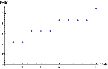
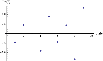
Figure 1: Real parts (left panel) and imaginary parts (right panel) of the first eleven energy levels of $H_{2}$ ($N=2$, $\gamma=1$).

The nature of the eigenfunctions associated with the first few energy levels is depicted in Fig. 2. The ground-state ($n_{1}=n_{2}=0$) and the third-exited-state ($n_{1}=n_{2}=1$) eigenfunctions are partially $\mathcal{PT}$ symmetric, as can be seen in the left upper and lower diagrams, while the eigenfunctions corresponding to the first and third (complex) eigenvalues ($n_{1}=0,\,n_{2}=1$ and $n_{1}=0,\,n_{2}=2$), which are not partially $\mathcal{PT}$ symmetric are shown on the right diagrams.

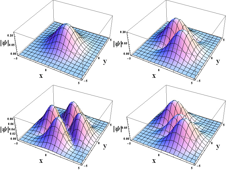
Figure 2: (Color online) Absolute value of the eigenfunction for the ground state (upper left), $n_{1}=n_{2}=1$ (lower left), $n_{1}=0,\,n_{2}=1$ (upper right) and $n_{1}=0,\,n_{2}=2$ (lower right) for $\gamma=1$.

III.2 Three coupled oscillators

To find the exact solution to the Schrödinger equation for $H_{3}$ in (5) with $\omega_{j}=1$ we make the transformation $x_{1}=(x-z)/\sqrt{2}$, $x_{2}=y/\sqrt{2}+(x+z)/2$, $x_{3}=-y/\sqrt{2}+(x+z)/2$, which decouples the oscillators, giving $H={\textstyle{\frac{1}{2}}}p_{1}^{2}+{\textstyle{\frac{1}{2}}}\nu_{1}^{2}x_{1}^{2}+{\textstyle{\frac{1}{2}}}p_{2}^{2}+{\textstyle{\frac{1}{2}}}\nu_{2}^{2}x_{2}^{2}+{\textstyle{\frac{1}{2}}}p_{3}^{2}+{\textstyle{\frac{1}{2}}}\nu_{3}^{2}x_{3}^{2}$ with $\nu_{1}^{2}=1$, $\nu_{2}^{2}=1+i\gamma\sqrt{2}$, and $\nu_{3}^{2}=1-i\gamma\sqrt{2}$. Thus, the unnormalized eigenfunctions are

$$\Psi(x_{1},x_{2},x_{3})=\mathcal{H}_{n_{1}}(x_{1})\mathcal{H}_{n_{2}}(\sqrt{\nu_{2}}x_{2})\mathcal{H}_{n_{3}}(\sqrt{\nu_{3}}x_{3})\exp\left[-(x_{1}^{2}+\nu_{2}x_{2}^{2}+\nu_{3}x_{3}^{2})/2\right]$$

and the energies are $E=n_{1}+{\textstyle{\frac{1}{2}}}+\nu_{2}\left(n_{2}+{\textstyle{\frac{1}{2}}}\right)+\nu_{3}\left(n_{3}+{\textstyle{\frac{1}{2}}}\right)$, where

$$\nu_{2,3}=\left({\textstyle{\frac{1}{2}}}+{\textstyle{\frac{1}{2}}}\sqrt{1+2\gamma^{2}}\right)^{1/2}\pm i\left(-{\textstyle{\frac{1}{2}}}+{\textstyle{\frac{1}{2}}}\sqrt{1+2\gamma^{2}}\right)^{1/2}.$$

Thus, the energy spectrum can be expressed as

$$E=n_{1}+{\textstyle{\frac{1}{2}}}+\sqrt{{\textstyle{\frac{1}{2}}}+{\textstyle{\frac{1}{2}}}\sqrt{1+2\gamma^{2}}}+\sqrt{{\textstyle{\frac{1}{2}}}+{\textstyle{\frac{1}{2}}}\sqrt{1+2\gamma^{2}}}\,\left(n_{2}+n_{3}\right)+i\sqrt{-{\textstyle{\frac{1}{2}}}+{\textstyle{\frac{1}{2}}}\sqrt{1+2\gamma^{2}}}\,\left(n_{2}-n_{3}\right).$$

Evidently, if the second and third oscillators are in the same state ($n_{2}=n_{3}$), the energy is real and the corresponding eigenfunctions are partially $\mathcal{PT}$ symmetric. In particular, the ground-state energy (6) is recovered and the ground-state eigenfunction is

$$\Psi_{0,0,0}(x,y,z)=\exp\left[-(1+a)(x^{2}+z^{2})/4-ay^{2}/2-(a-1)xz/2-ib(xy+yz)/\sqrt{2}\right],$$

where $a={\rm Re}\,\nu_{2}$, $b={\rm Im}\,\nu_{2}$. The first ten energies of $H_{3}$ for $\gamma=1$ are shown in Fig. 3.

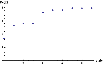
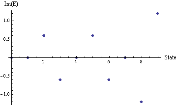
Figure 3: Real parts (left panel) and imaginary parts (right panel) of the first ten energies for $H_{3}$ ($\gamma=1$, $N=3$).

III.3 Four coupled oscillators

For the Hamiltonian (7), which governs four linearly coupled oscillators, the transformation

$$x_{1,2} = \frac{1}{2\sqrt{5}}\left[\sqrt{5-\sqrt{5}}\,(x\pm w)\pm\sqrt{5+\sqrt{5}}\,(y\pm z)\right],$$

$$x_{3,4} = \frac{1}{2\sqrt{5}}\left[\sqrt{5+\sqrt{5}}\,(x\mp w)\pm\sqrt{5-\sqrt{5}}\,(y\mp z)\right]$$

exactly decouples the oscillators. The new Hamiltonian takes the form

$$H={\textstyle{\frac{1}{2}}}p_{1}^{2}+{\textstyle{\frac{1}{2}}}\nu_{1}^{2}x_{1}^{2}+{\textstyle{\frac{1}{2}}}p_{2}^{2}+{\textstyle{\frac{1}{2}}}\nu_{2}^{2}x_{2}^{2}+{\textstyle{\frac{1}{2}}}p_{3}^{2}+{\textstyle{\frac{1}{2}}}\nu_{3}^{2}x_{3}^{2}+{\textstyle{\frac{1}{2}}}p_{4}^{2}+{\textstyle{\frac{1}{2}}}\nu_{4}^{2}x_{4}^{2},$$

where $\nu_{1}^{2}=\nu_{2}^{2*}=1+{\textstyle{\frac{1}{2}}}i\gamma(1+\sqrt{5})$ and $\nu_{3}^{2}=\nu_{4}^{2*}=1+{\textstyle{\frac{1}{2}}}i\gamma(-1+\sqrt{5})$ are complex frequencies. Let ${\rm Re}\,\nu_{1}={\rm Re}\,\nu_{2}=A$, ${\rm Re}\,\nu_{3}={\rm Re}\,\nu_{4}=C$, ${\rm Im}\,\nu_{1}=-{\rm Im}\,\nu_{2}=B$, ${\rm Im}\,\nu_{3}=-{\rm Im}\,\nu_{4}=D$, where

$$(A,B)=\sqrt{\pm{\textstyle{\frac{1}{2}}}+{\textstyle{\frac{1}{2}}}\sqrt{1+{\textstyle{\frac{1}{2}}}\gamma^{2}(3+\sqrt{5})}},\quad(C,D)=\sqrt{\pm{\textstyle{\frac{1}{2}}}+{\textstyle{\frac{1}{2}}}\sqrt{1+{\textstyle{\frac{1}{2}}}\gamma^{2}(3-\sqrt{5})}}.$$

In terms of these variables and the quantum numbers $n_{1}$, $n_{2}$, $n_{3}$, $n_{4}$, the total energy is

$$E_{n_{1},n_{2},n_{3},n_{4}}=A(n_{1}+n_{2}+1)+C(n_{3}+n_{4}+1)+iB(n_{1}-n_{2})+iD(n_{3}-n_{4}).$$

Thus, if $n_{1}=n_{2}$ and $n_{3}=n_{4}$, the energy is real. When the energy is real, the corresponding eigenfunction is always $\mathcal{P}_{xz}\mathcal{T}$- or $\mathcal{P}_{yw}\mathcal{T}$- symmetric. For example, the ground-state energy is $E_{0,0,0,0}=A+C$ and the corresponding eigenfunction is

$$\Psi_{0,0,0,0}=\exp\left[-\frac{1}{4}\left(A+C+\frac{C-A}{\sqrt{5}}\right)\left(x^{2}+w^{2}\right)-\frac{1}{4}\left(A+C+\frac{A-C}{\sqrt{5}}\right)\left(y^{2}+z^{2}\right)\right.$$

$$-\frac{1}{\sqrt{5}}(A-C)(xz+yw)-\frac{i}{2}\left(B-\frac{B}{\sqrt{5}}-D-\frac{D}{\sqrt{5}}\right)xw-\frac{i}{2}\left(B+\frac{B}{\sqrt{5}}-D+\frac{D}{\sqrt{5}}\right)yz$$

$$-\left.\frac{i}{\sqrt{5}}(B+D)(xy+wz)\right].$$ (13)

This eigenfunction displays the symmetries assumed in the ansatz (8).

As another illustration, we consider the case in which the first two oscillators are in the first excited state, and the other two in the ground state ($n_{1}=n_{2}=1$, $n_{3}=n_{4}=0$). The energy is $E_{1,1,0,0}=3A+C$ and the eigenfunction is

$$\Psi_{1,1,0,0}=\frac{1}{5}\sqrt{A^{2}+B^{2}}\left[(5-\sqrt{5})(x^{2}-\omega^{2})-(5+\sqrt{5})(y^{2}-z^{2})+4\sqrt{5}xz-4\sqrt{5}yw\right]\Psi_{0,0,0,0}.$$

Once again, the energy is real and the eigenfunction is $\mathcal{P}_{xz}\mathcal{T}$- or $\mathcal{P}_{yw}\mathcal{T}$-symmetric. A complex energy $E_{1,0,0,0}=2A+C+iB$ arises for the choice $n_{1}=1$, $n_{2}=n_{3}=n_{4}=0$.

III.4 Five coupled oscillators

The Hamiltonian for five coupled oscillators is

$$H_{5}={\textstyle{\frac{1}{2}}}\left(p^{2}+q^{2}+r^{2}+s^{2}+t^{2}\right)+{\textstyle{\frac{1}{2}}}\left(x^{2}+y^{2}+z^{2}+w^{2}+u^{2}\right)+i\gamma(xy+yz+zw+wu).$$

Rather than decoupling the oscillators we treat this case by constructing the secular equation

$${\rm det}\left(M_{jk}-\nu^{2}\delta_{jk}\right)=0,$$ (14)

where $M_{jk}$ is the tridiagonal matrix defined as

$$M_{jk}\equiv\frac{\partial^{2}U}{\partial q_{j}\partial q_{k}}\bigg{|}_{0}=\left(\begin{array}[]{ccccc}1&i\gamma&0&0&0\\ i\gamma&1&i\gamma&0&0\\ 0&i\gamma&1&i\gamma&0\\ 0&0&i\gamma&1&i\gamma\\ 0&0&0&i\gamma&1\end{array}\right),$$ (15)

$U$ is the potential, and $q_{j}$ and $q_{k}$ are coordinates.

The solution to the secular equation (14) gives complex-conjugate pairs of frequencies and one real frequency: $\nu_{1,2}^{2}={1\pm i\gamma\sqrt{3}}$, $\nu_{3,4}^{2}={1\pm i\gamma}$, $\nu_{5}=1$. Thus, the decoupled Hamiltonian is

$$H={\textstyle{\frac{1}{2}}}p_{1}^{2}+{\textstyle{\frac{1}{2}}}\nu_{1}^{2}x_{1}^{2}+{\textstyle{\frac{1}{2}}}p_{2}^{2}+{\textstyle{\frac{1}{2}}}\nu_{2}^{2}x_{2}^{2}+{\textstyle{\frac{1}{2}}}p_{3}^{2}+{\textstyle{\frac{1}{2}}}\nu_{3}^{2}x_{3}^{2}+{\textstyle{\frac{1}{2}}}p_{4}^{2}+{\textstyle{\frac{1}{2}}}\nu_{4}^{2}x_{4}^{2}+{\textstyle{\frac{1}{2}}}p_{5}^{2}+{\textstyle{\frac{1}{2}}}x_{5}^{2}$$

and the energy of the system reads

$$E=\nu_{1}\left(n_{1}+{\textstyle{\frac{1}{2}}}\right)+\nu_{2}\left(n_{2}+{\textstyle{\frac{1}{2}}}\right)+\nu_{3}\left(n_{3}+{\textstyle{\frac{1}{2}}}\right)+\nu_{4}\left(n_{4}+{\textstyle{\frac{1}{2}}}\right)+n_{5}+{\textstyle{\frac{1}{2}}},$$

where $n_{1}$, $n_{2}$, $n_{3}$, $n_{4}$, $n_{5}$ are nonnegative integers.

III.5 General case: $N$ coupled oscillators with $\omega_{j}=1$

In this section we consider the Hamiltonian (1) for $N$ linearly coupled oscillators with $\omega_{j}=1$. To obtain the frequencies of the decoupled oscillators we use (14) to construct the $N\times N$ tridiagonal matrix secular equation, ${\rm det}(\mathbf{M}-\nu^{2}\mathbf{I})=0$, which has the form

$$D_{N}=\begin{vmatrix}1-\nu^{2}&i\gamma&&&&\\ i\gamma&1-\nu^{2}&i\gamma&&&\\ &i\gamma&1-\nu^{2}&i\gamma&&\\ &&\ddots&\ddots&\ddots&\\ &&&i\gamma&1-\nu^{2}&i\gamma\\ &&&&i\gamma&1-\nu^{2}\end{vmatrix}=0.$$

Because this matrix equation is tridiagonal, $D_{N}$ satisfies the three-term recurrence relation

$$D_{k}+\left(\nu^{2}-1\right)D_{k-1}-\gamma^{2}D_{k-2}=0\quad(k=1,2,\ldots,N),$$

where $D_{0}=1$ and $D_{-1}=0$. We solve this difference equation to obtain the frequencies

$$\nu^{2}=1+2i\gamma\cos[j\pi/(N+1)]\quad(j=1,2,\ldots,N).$$

Thus, the exact expression for the total energy of the system of $N$ oscillators is given by

$$E=\sum_{j=1}^{N}\sqrt{1+2i\gamma\cos[j\pi/(N+1)]}\,\left(n_{j}+{\textstyle{\frac{1}{2}}}\right),$$

where $n_{j}\geq 0$ ($j=1,...,N$). Choosing $n_{j}=0$ for all $j$, we find the exact ground-state energy in (11), which has been shown to be real.

IV Coupled oscillators with arbitrary frequencies

In Secs. II and III the oscillator frequencies multiplying $x_{j}^{2}$ were set to unity. Our conclusion in the foregoing analysis was that a real spectrum is embedded in a complex spectrum containing complex-conjugate pairs of energies. We now relax this constraint on the natural frequencies. For the two-, three-, and four-coupled-oscillator systems, we demonstrate that for an appropriate choice of $\omega_{j}$ the spectrum can be entirely real.

IV.1 Two coupled oscillators with general natural frequencies $\omega_{x}$ and $\omega_{y}$

The Hamiltonian $H_{2}$ in (1) reads $H_{2}={\textstyle{\frac{1}{2}}}p^{2}+{\textstyle{\frac{1}{2}}}q^{2}+{\textstyle{\frac{1}{2}}}\omega_{x}^{2}x^{2}+{\textstyle{\frac{1}{2}}}\omega_{y}^{2}y^{2}+i\gamma xy$. The frequencies of the decoupled oscillators in this case are

$$\nu_{1,2}^{2}={\textstyle{\frac{1}{2}}}\left({\omega_{x}^{2}+\omega_{y}^{2}\pm\sqrt{(\omega_{x}^{2}-\omega_{y}^{2})^{2}-4\gamma^{2}}}\right)$$ (16)

and the energies of the system are $E_{n_{1},n_{2}}=\nu_{1}\left(n_{1}+{\textstyle{\frac{1}{2}}}\right)+\nu_{2}\left(n_{2}+{\textstyle{\frac{1}{2}}}\right)$, where $n_{1},n_{2}\geq 0$.

In contrast to the results found in Sec. III, the entire energy spectrum can be real for specific values of $\omega_{x}$, $\omega_{y}$, and $\gamma$. For this to be so, the parameters must satisfy the condition

$$|\omega_{x}^{2}-\omega_{y}^{2}|\geq 2|\gamma|.$$ (17)

The case considered in Sec. III had $\omega_{x}=\omega_{y}=1$ and $\gamma=1$, which does not satisfy this condition and, as we saw, the energy spectrum was only partially real.

To have real eigenvalues the associated eigenfunctions must all be partially $\mathcal{PT}$ symmetric. This can be seen explicitly by decoupling the oscillators with the transformation

$$x_{1}=\sqrt{A+B}(Dx+Ex+iCy)/(2CE),\quad x_{2}=\sqrt{A-B}(-Dx+Ex-iCy)/(2CE),$$

where $A=8\gamma^{2}-2(w_{x}^{2}-w_{y}^{2})^{2}$, $B=2(w_{x}^{2}-w_{y}^{2})\big{[}(w_{x}^{2}-w_{y}^{2})^{2}-4\gamma^{2}\big{]}^{1/2}$, $C=2\gamma$, $D=w_{x}^{2}-w_{y}^{2}$, $E=\big{[}(w_{x}^{2}-w_{y}^{2})^{2}-4\gamma^{2}\big{]}^{1/2}$, leading to the Hamiltonian $H={\textstyle{\frac{1}{2}}}p_{1}^{2}+{\textstyle{\frac{1}{2}}}\nu_{1}^{2}x_{1}^{2}+{\textstyle{\frac{1}{2}}}p_{2}^{2}+{\textstyle{\frac{1}{2}}}\nu_{2}^{2}x_{2}^{2}$, where $\nu_{1}$ and $\nu_{2}$ are given in (16). Up to a normalization constant, the eigenfunctions are

$$\Psi_{n_{1},n_{2}}(x_{1},x_{2})=\mathcal{H}_{n_{1}}\left(\sqrt{\nu_{1}}x_{1}\right)\mathcal{H}_{n_{2}}\left(\sqrt{\nu_{2}}x_{2}\right)\exp\left(-{\textstyle{\frac{1}{2}}}\nu_{1}x_{1}^{2}-{\textstyle{\frac{1}{2}}}\nu_{2}x_{2}^{2}\right).$$

Note that $A+B$ and $A-B$ have opposite signs in the $\mathcal{PT}$-symmetric phase and that $A-B<0$. Rewriting $\Psi_{n_{1},n_{2}}(x_{1},x_{2})$ in terms of the original variables $x$ and $y$, one can show that the eigenfunction $\Psi_{n_{1},n_{2}}(x,y)$ has partial $\mathcal{PT}$ symmetry because

$$(\mathcal{P}_{x}\mathcal{T})\Psi_{n_{1},n_{2}}(x,y)=(-1)^{n_{1}}\Psi_{n_{1},n_{2}}(x,y),\quad(\mathcal{P}_{y}\mathcal{T})\Psi_{n_{1},n_{2}}(x,y)=(-1)^{n_{2}}\Psi_{n_{1},n_{2}}(x,y).$$

To illustrate, we consider the case $\omega_{x}^{2}=3$, $\omega_{y}^{2}=1$, and $\gamma=1/2$. The relation (17) is satisfied and we find the purely real nondegenerate spectrum shown in Fig. 4. When $|\omega_{x}^{2}-\omega_{y}^{2}|<2|\gamma|$, the energy spectrum is only partially real. Thus, there is a phase transition from the unbroken partially $\mathcal{PT}$-symmetric phase to the broken one. For example, keeping $\omega_{y}=1$ and $\gamma=1/2$, but adjusting $\omega_{x}^{2}$ so that it passes $2$, the first-excited-state energy becomes complex.

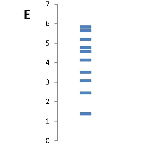
Figure 4: First ten energies of $H_{2}$ for the parameter choice $\omega_{x}^{2}=3$, $\omega_{y}^{2}=1$, and $\gamma=1/2$. These states have the quantum numbers $(n_{1},n_{2})=(0,0),(0,1),(1,0),(0,2),(1,1),(0,3),(2,0),(1,2),(0,4),(2,1)$.

IV.2 Three coupled oscillators with general natural frequencies $\omega_{x}$, $\omega_{y}$ and $\omega_{z}$

For the three-oscillator Hamiltonian $H_{3}={\textstyle{\frac{1}{2}}}p^{2}+{\textstyle{\frac{1}{2}}}q^{2}+{\textstyle{\frac{1}{2}}}r^{2}+{\textstyle{\frac{1}{2}}}\omega_{x}^{2}x^{2}+{\textstyle{\frac{1}{2}}}\omega_{y}^{2}y^{2}+{\textstyle{\frac{1}{2}}}\omega_{z}^{2}z^{2}+i\gamma(xy+yz)$ the frequencies $\nu^{2}=\lambda$ of the decoupled oscillators satisfy the cubic equation $f(\lambda)=0$, where

$$f(\lambda)=\lambda^{3}-\left(\omega_{x}^{2}+\omega_{y}^{2}+\omega_{z}^{2}\right)\lambda^{2}+\left(\omega_{x}^{2}\omega_{y}^{2}+\omega_{x}^{2}\omega_{z}^{2}+\omega_{y}^{2}\omega_{z}^{2}+2\gamma^{2}\right)\lambda-\omega_{x}^{2}\omega_{y}^{2}\omega_{z}^{2}-\left(\omega_{x}^{2}+\omega_{z}^{2}\right)\gamma^{2}.$$

If the discriminant associated with this equation is positive, three real distinct roots can emerge, giving a real spectrum. To guarantee that the roots are positive, it is necessary that

$$f(0)<0,\quad\lambda_{\rm max}>0,\quad\lambda_{\rm min}>0,\quad f(\lambda_{\rm max})>0,\quad f(\lambda_{\rm min})<0$$

are all fulfilled, with $\lambda_{\rm min}$ and $\lambda_{\rm max}$ being the extrema of the polynomial. Figure 5 displays the regions in which the frequencies of the decoupled oscillators are all real (blue shaded areas) in the parametric space of $\omega_{x}$ and $\omega_{z}$ for fixed values of $\gamma$ and $\omega_{y}^{2}$. This figure shows that several regions of unbroken symmetry exist. This is in contrast to the case of the two coupled oscillators.

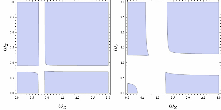
Figure 5: (Color online) Unbroken partial $\mathcal{PT}$-symmetric phases of $H_{3}$ depicted as shaded areas for the parameters $\gamma={1}/{12}$ and $\omega_{y}^{2}={2}/{3}$ (left panel) and $\gamma={1}/{3}$ and $\omega_{y}^{2}=1$ (right panel).

For example, Figure 5 shows that $\omega_{x}^{2}=1/3$, $\omega_{y}^{2}=2/3$, $\omega_{z}^{2}=1$, and $\gamma=1/12$ gives an unbroken symmetry phase. We obtain three different real positive (decoupled) frequencies

$$\nu_{1}=\sqrt{2/3},\quad\nu_{2}=\sqrt{(8+\sqrt{14})/12},\quad\nu_{3}=\sqrt{(8-\sqrt{14})/12}.$$

Thus, the spectrum is entirely real with energies given by $E_{n_{1},n_{2},n_{3}}=\nu_{1}\left(n_{1}+{\textstyle{\frac{1}{2}}}\right)+\nu_{2}\left(n_{2}+{\textstyle{\frac{1}{2}}}\right)+\nu_{3}\left(n_{3}+{\textstyle{\frac{1}{2}}}\right)$. By fixing only $\gamma$ we can find regions in the three-dimensional parameter space of $\omega_{x}$, $\omega_{y}$, and $\omega_{z}$ for which unbroken symmetry (and therefore a real spectrum) exists. This is shown in the colored volumes depicted in Fig. 6 for the specific choice $\gamma=1/12$.

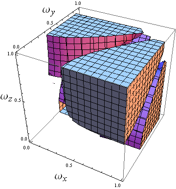
Figure 6: (Color online) Unbroken partial $\mathcal{PT}$-symmetric phases of $H_{3}$ for $\gamma=1/12$ depicted as colored volumes.

IV.3 Four coupled oscillators with general natural frequencies $\omega_{x}$, $\omega_{y}$, $\omega_{z}$, and $\omega_{w}$

The previous analysis can be applied to the four-coupled-oscillator Hamiltonian

$$H_{4}={\textstyle{\frac{1}{2}}}p^{2}+{\textstyle{\frac{1}{2}}}q^{2}+{\textstyle{\frac{1}{2}}}r^{2}+{\textstyle{\frac{1}{2}}}s^{2}+{\textstyle{\frac{1}{2}}}\omega_{x}^{2}x^{2}+{\textstyle{\frac{1}{2}}}\omega_{y}^{2}y^{2}+{\textstyle{\frac{1}{2}}}\omega_{z}^{2}z^{2}+{\textstyle{\frac{1}{2}}}\omega_{w}^{2}w^{2}+i\gamma(xy+yz+zw),$$

where $\omega_{x}$, $\omega_{y}$, $\omega_{z}$, and $\omega_{w}$ are real frequencies and $\gamma$ is a real coupling parameter.

The eigenvalues of the matrix

$$M=\left(\begin{array}[]{cccc}\omega_{x}^{2}&i\gamma&0&0\\ i\gamma&\omega_{y}^{2}&i\gamma&0\\ 0&i\gamma&\omega_{z}^{2}&i\gamma\\ 0&0&i\gamma&\omega_{w}^{2}\end{array}\right)$$

are the squares of the corresponding decoupled-oscillator frequencies. The eigenvalues $\nu^{2}=\lambda$ satisfy the fourth-order equation $f(\lambda)=\lambda^{4}-a\lambda^{3}+b\lambda^{2}-c\lambda+d=0$, where

$$a =\omega_{x}^{2}+\omega_{y}^{2}+\omega_{z}^{2}+\omega_{w}^{2},$$

$$b =\omega_{x}^{2}\omega_{y}^{2}+\omega_{x}^{2}\omega_{z}^{2}+\omega_{x}^{2}\omega_{w}^{2}+\omega_{y}^{2}\omega_{z}^{2}+\omega_{y}^{2}\omega_{w}^{2}+\omega_{z}^{2}\omega_{w}^{2}+3\gamma^{2},$$

$$c =\omega_{x}^{2}\omega_{y}^{2}\omega_{z}^{2}+\omega_{x}^{2}\omega_{y}^{2}\omega_{w}^{2}+\omega_{x}^{2}\omega_{z}^{2}\omega_{w}^{2}+\omega_{y}^{2}\omega_{z}^{2}\omega_{w}^{2}+2\gamma^{2}\omega_{x}^{2}+2\gamma^{2}\omega_{w}^{2}+\gamma^{2}\omega_{y}^{2}+\gamma^{2}\omega_{z}^{2},$$

$$d =\omega_{x}^{2}\omega_{y}^{2}\omega_{z}^{2}\omega_{w}^{2}+\gamma^{2}\omega_{x}^{2}\omega_{y}^{2}+\gamma^{2}\omega_{x}^{2}\omega_{w}^{2}+\gamma^{2}\omega_{z}^{2}\omega_{w}^{2}+\gamma^{4}.$$

Regions in which all decoupled oscillator frequencies are real give a completely real energy spectrum, which means that partial $\mathcal{PT}$ symmetry is unbroken. This requires that $f(\lambda)$ have four positive roots, which is the case if $f(0)>0$. In addition, if $f^{\prime}(\lambda)$ has three positive roots, the extrema of $f(\lambda)$ lie on the positive abscissa. To have four real roots the minimum value of $f(\lambda)$ must be negative, and the maximum value must be positive. Figure 7 shows the regions in which these conditions are fulfilled (that is, the regions in which the partial $\mathcal{PT}$ symmetry is unbroken) for specific choices of the parameters. Fixing the values of $\omega_{z}^{2}=1$ and $\omega_{w}^{2}=4$ as in the right panel of Fig. 7, we can investigate the development of the phase boundaries as a function of the coupling strength $\gamma$. This is shown in Fig. 8.

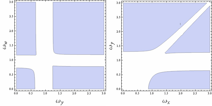
Figure 7: (Color online) Unbroken partial $PT$-symmetric phases of $H_{4}$ depicted as shaded area. Left panel: $\gamma=1/5$, $\omega_{x}^{2}=1$, and $\omega_{z}^{2}=1$. Right panel: $\gamma=3/10$, $\omega_{z}^{2}=1$, and $\omega_{w}^{2}=4$.

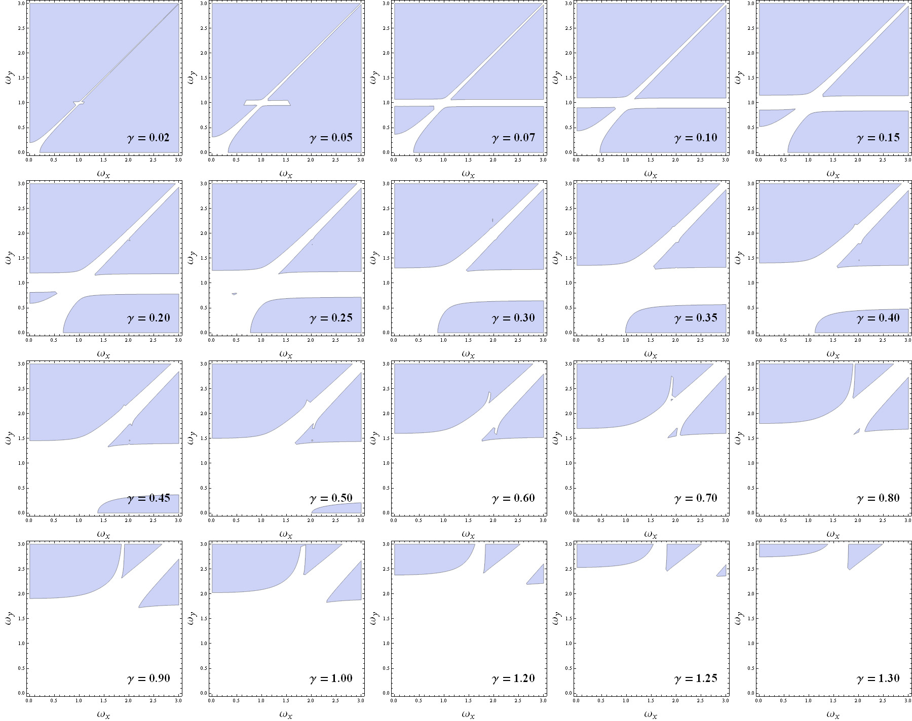
Figure 8: (Color online) Unbroken partial $PT$-symmetric phases of $H_{4}$ in the $(\omega_{x},\omega_{y})$ plane depicted as shaded areas for the parameter choices $\omega_{z}^{2}=1$ and $\omega_{w}^{2}=4$ for twenty values of $\gamma$.

V Corresponding Classical Theory

In this section we investigate the features of partially $\mathcal{PT}$-symmetric classical theories. We begin with the two-coupled-oscillator Hamiltonian $H_{2}$ with frequencies $\omega_{x}=\omega_{y}=1$. Hamilton’s classical equations of motion lead to

$$x^{\prime\prime}(t)+x(t)+i\gamma y(t)=0,\quad y^{\prime\prime}(t)+y(t)+i\gamma x(t)=0$$

and combining these equations gives the fourth-order differential equation

$$x^{\prime\prime\prime\prime}(t)+2x^{\prime\prime}(t)+(1+\gamma^{2})x(t)=0.$$

We seek solutions $x(t)=e^{i\nu t}$ and find that $\lambda=\nu^{2}$ satisfies the quadratic equation $\lambda^{2}-2\lambda+1+\gamma^{2}=0$, so $\nu=\pm\sqrt{1\pm i\gamma}$. Thus, the characteristic frequencies are always complex. By decomposing $\sqrt{1+i\gamma}=a+ib$ into its real and imaginary parts we can write the general solution as

$$x(t)=\left[(A+D)e^{-bt}+(B+C)e^{bt}\right]\cos(at)+i\left[(A-D)e^{-bt}+(B-C)e^{bt}\right]\sin(at),$$

where $A$, $B$, $C$ and $D$ are arbitrary constants. Therefore, for any initial conditions, the real and imaginary parts of $x(t)$ are oscillatory and growing (or decreasing). As a consequence, the trajectories in the complex-$x$ plane spiral outward (or inward). Hence, the classical paths are open (see Fig. 9, left panel). Thus, although the quantum spectrum is partially real, this partial reality does not give rise to closed classical trajectories.

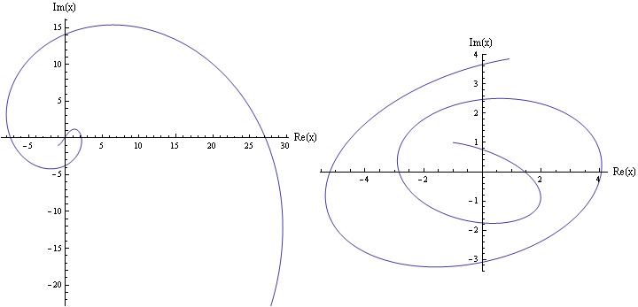
Figure 9: Left panel: classical trajectory in the complex-$x$ plane for $H_{2}$ with $\omega_{x}^{2}=\omega_{y}^{2}=1$ with the initial conditions $x(0)=y(0)=-1-i$ and $\dot{x}(0)=\dot{y}(0)=1+i/2$, and $\gamma=1$. Right panel: Classical trajectory in the complex-$x$ plane for $H_{2}$ with $\omega_{x}^{2}=2$, $\omega_{y}^{2}=1$, and $\gamma=1/2$ for the initial conditions $x(0)=y(0)=-1+i$ and $\dot{x}(0)=\dot{y}(0)=2-i/4$.

More generally, if the coupled oscillators described by $H_{2}$ have natural frequencies $\omega_{x}$ and $\omega_{y}$, we obtain the equation

$$x^{\prime\prime\prime\prime}(t)+\left(w_{x}^{2}+w_{y}^{2}\right)x^{\prime\prime}(t)+\left(w_{x}^{2}w_{y}^{2}+\gamma^{2}\right)x(t)=0.$$

Again seeking solutions $x(t)=e^{i\nu t}$, we find that $\nu^{2}={\textstyle{\frac{1}{2}}}w_{x}^{2}+{\textstyle{\frac{1}{2}}}w_{y}^{2}\pm{\textstyle{\frac{1}{2}}}\big{[}(\omega_{x}^{2}-\omega_{y}^{2})^{2}-4\gamma^{2}\big{]}^{1/2}$. We deduce that four real values of $\nu$ exist when $|\omega_{x}^{2}-\omega_{y}^{2}|\geq 2|\gamma|$, which is precisely the condition that guarantees a fully real spectrum in the quantum system [see (17)]. Thus, the transition from the broken partial-$\mathcal{PT}$-symmetric phase to the unbroken phase occurs at the same point as for the quantum case. For the parameter choice $\omega_{x}^{2}=2$, $\omega_{y}^{2}=1$, and $\gamma=1/2$ the classical trajectory depicted in Fig. 9 (right panel) spirals outward, which indicates that $\mathcal{PT}$ symmetry is broken even though the system is partially $\mathcal{PT}$ symmetric. The behavior of the trajectories in the unbroken phase is illustrated in Fig. 10. Here, one sees that while the classical trajectory is not closed it is confined to a compact region in the complex-$x$ plane. We thus observe the phase transition at the classical level; that is, we observe the transition from spirals (broken phase) to localized trajectories in the complex-$x$ plane (unbroken phase), which happens at $|\omega_{x}^{2}-\omega_{y}^{2}|=2|\gamma|$.

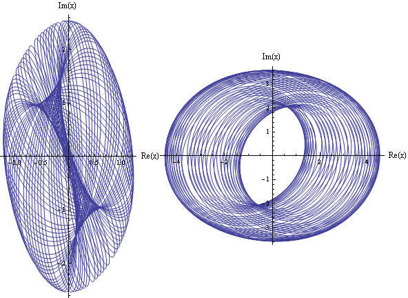
Figure 10: Classical trajectory in the complex-$x$ plane for $H_{2}$ with the parameter choice $\omega_{x}^{2}=3$, $\omega_{y}^{2}=1$, $\gamma=1/2$, with the initial conditions $x(0)=-1+i$, $y(0)=2-2i$, $\dot{x}(0)=1+i/2$, $\dot{y}(0)=3/2+i$ (left panel) and $x(0)=1+2i$, $y(0)=2+i/4$, $\dot{x}(0)=-3+i$, $\dot{y}(0)=1/2+5i$ (right panel).

In addition to studying the trajectory in the complex-$x$ plane, one can study the trajectories in phase space by plotting a Poincaré section. From the structure of the Poincaré plot we conclude that the confined trajectories are almost periodic BO . This is illustrated in Fig. 11. The appearance of open almost-periodic trajectories occurs because the number of degrees of freedom exceeds one; if $N=1$, the classical orbits associated with real quantum energies are closed BBH .

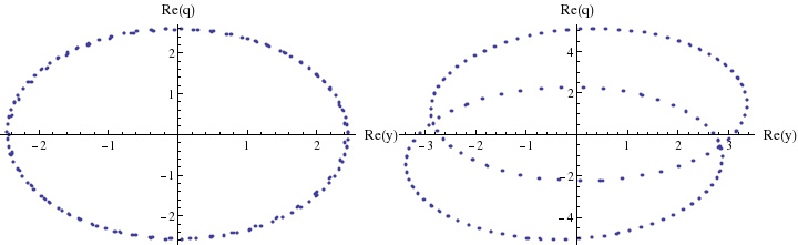
Figure 11: Poincaré section of the classical trajectory in phase space for $H_{2}$ with the parameter choice $\omega_{x}^{2}=3$, $\omega_{y}^{2}=1$, $\gamma=1/2$ and initial conditions $x(0)=1+i/2$, $y(0)=-2+2i$, $\dot{x}(0)=1+i/2$, $\dot{y}(0)=-3/2-3i/2$ (left panel) and $x(0)=2+5i/2$, $y(0)=2-3i$, $\dot{x}(0)=1-i/2$, $\dot{y}(0)=2-2i$ (right panel). The structure of this plot indicates that the orbits are almost periodic.

A similar analysis can be done for the three-coupled-oscillator Hamiltonian $H_{3}$ with general natural frequencies. The classical equations of motion are

$$x^{\prime\prime}(t)+\omega_{x}^{2}x(t)+i\gamma y(t)=0,\quad y^{\prime\prime}(t)+\omega_{y}^{2}y(t)+i\gamma(x(t)+z(t))=0,\quad z^{\prime\prime}(t)+\omega_{z}^{2}z(t)+i\gamma y(t)=0.$$

Seeking solutions of the form $x(t)=Ae^{i\nu t}$, $y(t)=Be^{i\nu t}$ and $z(t)=Ce^{i\nu t}$, we obtain a cubic equation for $\lambda=\nu^{2}$:

$$\lambda^{3}-\left(\omega_{x}^{2}+\omega_{y}^{2}+\omega_{z}^{2}\right)\lambda^{2}+\left(\omega_{x}^{2}\omega_{y}^{2}+\omega_{x}^{2}\omega_{z}^{2}+\omega_{y}^{2}\omega_{z}^{2}+2\gamma^{2}\right)\lambda-\omega_{x}^{2}\omega_{y}^{2}\omega_{z}^{2}-\left(\omega_{x}^{2}+\omega_{z}^{2}\right)\gamma^{2}=0.$$

The characteristic frequencies are real if and only if the corresponding quantum system is in an unbroken $\mathcal{PT}$-symmetric phase (all eigenvalues are real); the criteria for real eigenvalues is given in Sec. IV. To illustrate, recall that in Sec. IV the parameter choice $\omega_{x}^{2}=1/3$, $\omega_{y}^{2}=2/3$, $\omega_{z}^{2}=1$, $\gamma=1/12$ lies in the unbroken phase and gives a real energy spectrum. Figure 12 shows that for this parameter choice, the classical trajectory is confined to a compact region in the complex-$x$ plane, whereas for the choice $\omega_{x}^{2}=1/3$, $\omega_{y}^{2}=2/3$, $\omega_{z}^{2}=13/20$, and $\gamma=1/12$, for which the quantum symmetry is broken, the classical trajectory spirals outward to infinity. A Poincaré section is given in Fig. 13 for the parameter choice of Fig. 12, left panel.

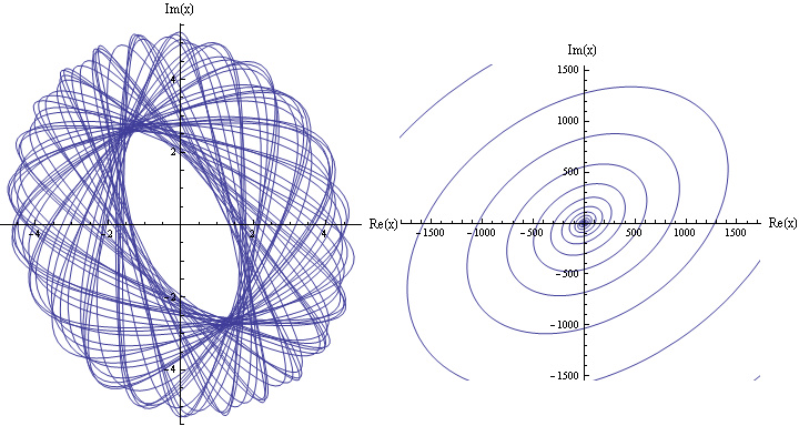
Figure 12: Classical trajectory in the complex-$x$ plane for $H_{3}$ with the parameter choice $\omega_{x}^{2}=1/3$, $\omega_{y}^{2}=2/3,\gamma=1/12$, $\omega_{z}^{2}=1$ (left panel) and $\omega_{z}^{2}=13/20$ (right panel) with the initial conditions $x(0)=-2+i$, $y(0)=3-3i$, $z(0)=3+2i$, $\dot{x}(0)=-1+3i$, $\dot{y}(0)=3+2i$, $\dot{z}(0)=-2+i$.

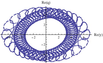
Figure 13: Poincaré section of the classical trajectory for $H_{3}$ with the parameter choice $\omega_{x}^{2}=1/3$, $\omega_{y}^{2}=2/3$, $\omega_{z}^{2}=1$, $\gamma=1/12$ and the initial conditions $x(0)=-2+i$, $y(0)=3-3i$, $z(0)=3+2i$, $\dot{x}(0)=-1+3i$, $\dot{y}(0)=3+2i$, $\dot{z}(0)=-2+i$. This figure indicates that the orbit is almost periodic.

VI Brief concluding remarks

In this paper we have examined systems of $N$ linearly coupled oscillators that are partially $\mathcal{P}\mathcal{T}$-symmetric. In the quantum-mechanical analysis we have found that the ground state of each of these systems is always real. We have shown that the entire spectrum may in fact be completely real depending on the values of the natural frequencies $\omega_{x}$, $\omega_{y}$, $\omega_{z}$, $\dots$ and their relation to the coupling strength $\gamma$. This happens even though the system is only partially $\mathcal{PT}$ symmetric. We have studied this in detail for systems of two and three coupled oscillators. A phase transition point exists beyond which the energy spectrum is only partially real.

For the two and three classical oscillator systems, we find a phase transition at exactly the same point as the quantum-mechanical oscillator systems. When the eigenvalues of the quantum system are all real, the classical trajectories are confined and almost periodic, but when the quantum eigenvalues are partly real and partly complex, the corresponding classical system always has open trajectories that spiral out to infinity.

- (1) J. Schindler, A. Li, M. C. Zheng, F. M. Ellis, and T. Kottos, Phys. Rev. A 84, 040101 (2011).
- (2) C. M. Bender, B. Berntson, D. Parker, and E. Samuel, Am. J. Phys. 81, 173 (2013).
- (3) C. M. Bender, M. Gianfreda, S. K. Özdemir, B. Peng, and L. Yang, Phys. Rev. A 88, 062111 (2013).
- (4) J. Cuevas, P. G. Kevrekidis, A. Saxena, and A. Khare, Phys. Rev. A 88, 032108 (2013).
- (5) C. M. Bender, M. Gianfreda, and S. P. Klevansky, Phys. Rev. A 90, 022114 (2014).
- (6) B. Peng, S. K. Özdemir, F. Lei, F. Monifi, M. Gianfreda, G. L. Long, S. Fan, F. Nori, C. M. Bender, L. Yang, Nat. Phys. 10, 394 (2014).
- (7) I. L. Aleiner, B. L. Altshuler, and Y. G. Rubo, Phys. Rev. B 85, 121301 (2012).
- (8) C. M. Bender and S. A. Orszag, Advanced Mathematical Methods for Scientists and Engineers (McGraw-Hill, New York, 1978).
- (9) C. M. Bender, D. C. Brody, and D. W. Hook, J. Phys. A: Math. Theor. 41, 352003 (2008).