Analytical Study of Quantum Feedback Enhanced Rabi Oscillations

Abstract

We present an analytical solution of the single photon quantum feedback in a cavity quantum electrodynamics system based on a half cavity set-up coupled to a structured continuum. The exact analytical expression we obtain allows us to discuss in detail under which conditions a single emitter-cavity system, which is initially in the weak coupling regime, can be driven into the strong coupling regime via the proposed quantum feedback mechanism [Carmele et al, Phys.Rev.Lett. 110, 013601]. Our results reveal that the feedback induced oscillations rely on a well-defined relationship between the delay time and the atom-light coupling strength of the emitter. At these specific values the leakage into the continuum is prevented by a destructive interference effect, which pushes the emitter to the strong coupling limit.

March 14, 2024

I Introduction

The basic phenomenon at the heart of any quantum information processing network is the coherent exchange of photonic and atomic excitations by means of a single emitter in a microcavity. Advances in the design and fabrication of microcavities allow very high quality factors and have enabled multiple studies of cavity quantum electrodynamics (cQED) in the strong coupling limit Hennessy et al. (2007); McKeever et al. (2003); Putz et al. (2014); Krimer et al. (2014a); Fink et al. (2008); Schuster et al. (2008). Several applications are proposed and already realized, such as single-photon transistors, two-photon gateways, parametric downconversion as well as the generation and detection of individual microwave photons Chang et al. (2007); Nielsen and Chuang (2000); Monroe (2002); Zoller et al. (2005). Furthermore, several quantum gate proposals rely on a natural quantum interface between flying qubits (photons) and stationary qubits (e.g. atoms). Here, the photons allow for secure quantum communication over long distances, whereas atoms can be used for the manipulation and storage of quantum information Zoller et al. (2005).
Applying cQED techniques require that a single-atom/single-photon coupling exceeds any photon loss and radiative decay processes, such as spontaneous emission or photon leakage. So, besides technological progress to increase the quality factor of the cavities, a promising alternative is to identify strategies to control and exploit potentially advantageous properties of the environment coupling, which go beyond the conventional effects of the environment like dissipation and undesired information loss.
A possible mechanism to stabilize qubits and desired quantum states is quantum feedback based on the repeated action of a sensor-controller-actuator loop. In such a case, a quantum system is driven to a target state via the external control Zhou et al. (2012); Wiseman and Milburn (2006), such that continuous measurements allow to stabilize the target state, e.g. by a modification of the pumping strength. In addition to these extrinsic control set-ups, experiments start to explore a variety of intrinsic, delayed feedback control schemes, e.g., by using an external mirror in front of a nanocavity Albert et al. (2011). Intrinsic quantum feedback is not based on a continuous measurement process, but controls the quantum state by shaping the environment appropriately Kopylov et al. (2015); Grimsmo et al. (2014); Strasberg et al. (2013); Pyragas and Novičenko (2013); Hein et al. (2014); Schulze et al. (2014); Carmele et al. (2013).
Here, we discuss the photon leakage mechanism shaped by an external mirror and show analytically, how the initial weak atom-cavity coupling is driven into the strong coupling regime, following Ref. Carmele et al. (2013). Our proposed control scheme has potential applications for quantum error correction Shor (1995), quantum gate purifying van Enk et al. (1997), or quantum feedback Wiseman and Milburn (2006).

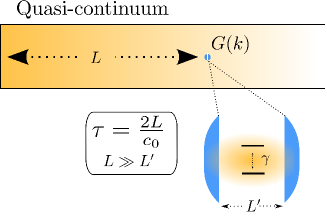
Figure 1: Implementation of an intrinsic quantum feedback mechanism via a quasi-continuum, realized by a photonic crystal waveguide with length $L$, which is supposed to be considerably larger than the cavity length $L^{\prime}$. The waveguide is a half-cavity and allows to exchange cavity photons with waveguide photons due to the photon leakage $G(k)$. The photons inside the cavity interact with a single emitter (coupling strength $\gamma$).

II Model

The system consists of a microcavity system of length $L^{\prime}$ with a two-level emitter coupled to a single cavity mode (see Fig. 1). Furthermore, the cavity exhibits photon loss due to its coupling to external modes. An external mirror, placed in a distance of $L$, introduces a boundary condition to the external mode structure and causes a feedback of lost cavity photons into the cavity. We assume that the microcavity length $L^{\prime}\ll L$ is very short in comparison to $L$ to allow a single mode description for the emitter-cavity interaction. This kind of quantum self-feedback can be realized via a shaped mode continuum in a photonic waveguide. Due to the finite cavity-mirror distance $L$ and the quasi-continuous mode structure of the semi-infinite lead, a delay mechanism is introduced into the system at $\tau=\frac{2L}{c_{0}}$ with $c_{0}$ being the speed of light in vacuum. To describe the corresponding physics we work with the following Hamiltonian within the rotating-wave and dipole approximation Walls and Milburn (2007):

$$H/\hbar = -\gamma\left(\sigma^{-}a^{\dagger}+\sigma^{+}a\right)$$

$$-\int\text{d}k\ G(k,t)\ a^{\dagger}d^{\phantom{\dagger}}_{k}+G^{*}(k,t)\ d^{\dagger}_{k}a,$$

where a rotating frame is chosen in correspondence to the free energy contribution of the Hamiltonian. The emitter is described via the Pauli matrices with $\sigma^{+/-}$ being the raising and lowering operators of the two level system, respectively. In the following, the atomic energy is assumed to be in resonance with the single cavity mode. A photon annihilation (creation) in the cavity is described with the bosonic operator $a^{\dagger}(a)$ and $\gamma$ is the coupling between the two-level system and the cavity mode. The coupling strength between the emitter and the field mode is assumed to be of the order of $\gamma=50\leavevmode\nobreak\ \mu$eV McKeever et al. (2003); Laucht et al. (2011); Berger et al. (2014). The cavity photons interact with the external modes $d^{(\dagger)}_{k}$ in front of the mirror via the tunnel Hamiltonian coupling elements $G(k,t)$. Due to the rotating frame and the interference with the back-reflected signal from the mirror, these coupling elements depend both on time $t$ and on the wavenumber $k$, resulting in the following expression for $G(k,t)=G_{0}\sin(kL)\exp[i(\omega_{0}-\omega_{k})t]$ with $G_{0}$ being the bare tunnel coupling strength. $\omega_{0}$ and $\omega_{k}$ stand for the frequencies of a single cavity mode and half-cavity modes, respectively. As we will see below, this specific form of $G(k,t)$ will determine the nature of the feedback on the cavity.

II.1 Single photon limit

If no other loss channels or pump mechanism are introduced, the system dynamics described by the Hamiltonian Eq. (II) can be solved in the Schrödinger picture, following Ref. Dorner and Zoller (2002); Cook and Milonni (1987). In the single photon limit, the total wave function reads:

$$|\Psi\rangle = c_{e}\left|e,0,\{0\}\right\rangle+c_{g}\left|g,1,\{0\}\right\rangle$$

$$+\int\text{d}k\ c_{g,k}\left|g,0,\{k\}\right\rangle,$$

where $\left|e,0,\{0\}\right\rangle$ denotes the excited state of the two-level system with the cavity and the waveguide being in the vacuum state, $\left|g,1,\{0\}\right\rangle$ stands for a single photon residing in the cavity and the two-level system as well as the radiation field in the waveguide being in the ground state. Finally, $\left|g,0,\{k\}\right\rangle$ describes the ground state of the two-level system with exactly one photon in the waveguide of mode $k$. The variables $c_{e},\,c_{g},\,c_{g,k}$ denote the corresponding amplitudes of the above three different states.
Applying the Schrödinger equation, we arrive at the following set of linear partial differential equations:

$$\partial_{t}c_{e} = i\ \gamma\ c_{g}$$ (3)

$$\partial_{t}c_{g} = i\ \gamma\ c_{e}+i\int\text{d}k\ \ G(k,t)\ c_{g,k}$$ (4)

$$\partial_{t}c_{g,k} = i\ G^{*}(k,t)\ c_{g}.$$ (5)

First, we numerically solve this coupled set of differential equations assuming that initially at $t_{0}=0$ the TLS is in the excited state, $c_{e}(t_{0})=1$, and there are neither photons inside the cavity, $c_{g}(t_{0})=0$, nor in the external region, $c_{g,k}(t_{0})=0$. To introduce a delay time corresponding to $\tau=2L/c_{0}=2\pi/\gamma$, we choose a mirror resonator distance $L=\pi c_{0}/\gamma$.

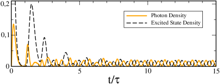
Figure 2: Excited state density $|c_{e}(t)|^{2}$ of the two-level system (black dashed line) and the photon density inside the cavity $|c_{g}(t)|^{2}$ (orange solid line) in the quasi-continuum model. The quantum feedback mechanism ($\kappa/\gamma=2$) induces a regular oscillation pattern at multiples of $\tau=2\pi/\gamma$.

The results for the dynamics of the excited state and photon density are shown in Fig. 2. In the time interval $[0,\tau]$ we find the conventional exponential decay as described by the Wigner-Weisskopf model in the weak coupling limit. After the first round trip $\tau=2L/c_{0}$, the photon density and after a small delay, also the excited state density, are driven by the quantum feedback. In this time interval $[\tau,2\tau]$, the amplitude of the photon density is smaller than the amplitude of the excited case, since the damping mechanism acts only on the photons inside the cavity. However, for longer times, the asymmetry between the amplitudes of the excited state and the photon density vanishes, so that the system sets into a state of coherent Rabi oscillations characterized by approximately equal maxima of both densities (see the asymptotic dynamics for $t/\tau\geq 8$ in Fig. 2). In this long-time limit, the amplitude for the cavity photon population stabilizes at around 15% of the maximum photon population in the first time interval ($[0,\tau]$). This remarkable effect has been reported in another publication Carmele et al. (2013) and will now be analyzed analytically and thereby explained in more detail. In particular, we will focus on the following two specific questions: (i) How sensitive is this effect on the chosen parameters, in particular on the choice of the time delay? (ii) Can the oscillation amplitude be increased or is there an intrinsic limit? To answer these questions, we will first derive a simplified picture of the dynamics by solving Eqs. (3)-(5) in the Markovian limit.

II.2 Analytical Quantum Feedback

The initial decay and the subsequent oscillations observable in Fig. 2 indicates that the underlying physical processes which govern this system consist both of a typical (Markovian) cavity loss as well as of a (non-Markovian) memory kernel with significant contributions around multiples of the delay time $\tau$. Assuming that the rotating wave approximation and the quasi-continuum assumption hold, the coupling to the external modes can be eliminated from the problem. To achieve this, Eq. (5) is integrated formally and inserted into Eq. (4) resulting in the following expression:

$$\partial_{t}c_{g} = i\ \gamma\ c_{e}-\kappa\ c_{g}+\kappa\ c_{g}\ \Theta(t-\tau)\ e^{i\omega_{0}\tau},$$ (6)

with $\kappa=\pi G_{0}^{2}/(2c_{0})$. This reduced expression has the advantage of being easily solvable numerically and of being amenable to an analytical solution through a Laplace transformation. With the initial conditions, that neither cavity nor continuum photons are present in the beginning, i.e. $c_{e}(0)=1$, the equations read after Laplace transformation:

$$\!\!\!\!\!\!\!\!s\ c_{e}(s) = 1+i\ \gamma\ c_{g}(s)$$ (7)

$$\!\!\!\!\!\!\!\!s\ c_{g}(s) = i\ \gamma\ c_{e}(s)-\kappa\ c_{g}(s)+\kappa\ c_{g}(s)\ e^{-(s-i\omega_{0})\tau},$$ (8)

where $s$ is the complex frequency parameter of the Laplace transformation. As can be seen from Eq. (6), the solution consists of a dynamical component without the mirror induced feedback $t\leq\tau$ and one with the feedback for $t>\tau$.

First, we now derive a solution for the photon-assisted ground state for $t\leq\tau$, which is the cavity damped Jaynes-Cummings model Gardiner and Zoller (1991):

$$c_{g}(s)=\frac{i\ \gamma}{s^{2}+\gamma^{2}+\kappa\ s}=\frac{i\ \gamma}{(s+\kappa/2)^{2}+\gamma^{2}-\kappa^{2}/4}.$$ (9)

This leads directly to the damped Jaynes-Cummings solutions in the time domain as expected for times $t\leq\tau$, when the cavity-system is not affected by the feedback mechanism:

$$c_{g}(t) = i\ \frac{\sin\left[\sqrt{1-(\kappa/2\gamma)^{2}}\ \gamma t\right]}{\sqrt{1-(\kappa/2\gamma)^{2}}}\ e^{-\kappa/2\ t}.$$ (10)

Note, due to the cavity damping not only the amplitude is reduced but also the Rabi oscillation frequency is reduced by a factor of $\sqrt{1-(\kappa/2\gamma)^{2}}$. The cavity loss leads inevitably to an effectively reduced value for the coupling strength, and as a result, the frequency of damped Rabi oscillations decreases. As we will see below, this restriction is lifted if a feedback mechanism is present.
Now, we solve the dynamics for times $t>\tau$. This leads to an additional term in the denominator. By using a geometric series expansion, i.e. $(1-q)^{-1}=\sum_{n}q^{n}$ for $q<1$ and $n\rightarrow\infty$, Eq. (9) can be written as:

$$c_{g}(s) = i\ \gamma\frac{\left[1-\frac{\kappa\ s\ \exp[-(s-i\omega_{0})\tau]}{(s+\kappa/2)^{2}+\gamma^{2}-\kappa^{2}/4}\right]^{-1}}{(s+\kappa/2)^{2}+\gamma^{2}-\kappa^{2}/4}$$

$$= i\ \gamma\sum_{n}\frac{\left[\frac{\kappa\ s\ \exp[-(s-i\omega_{0})\tau]}{(s+\kappa/2)^{2}+\gamma^{2}-\kappa^{2}/4}\right]^{n}}{(s+\kappa/2)^{2}+\gamma^{2}-\kappa^{2}/4}.$$

Due to the linearity of the Laplace transformation, the solution in the time domain can be obtained via the method of partial fraction expansion and the convolution property.

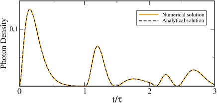
Figure 3: Comparison between numerical calculation and the Laplace transformed analytical solution valid until $t=3\tau$ with $\kappa/\gamma=2$.

However, the expression is very lengthy and must be calculated for every time interval $[n\tau,(n+1)\tau]$, separately. Since we are interested in the weak coupling regime, we can choose the parameter to be: $\gamma=\kappa/2$ to simplify the expression into:

$$c_{g}(s)\!=\!\frac{i\ \kappa/2}{(s+\kappa/2)^{2}}\!\sum_{n}\left[\frac{\kappa se^{(i\omega_{0}-s)\tau}}{(s+\kappa/2)^{2}}\right]^{n}.$$ (12)

Using now the binomial series and Laplace transformation: $n!/(s-a)^{n+1}\rightarrow t^{n}\exp[at]$, we get an expression in the time domain:

$$c_{g}(t) = \frac{i}{2}\sum_{n=0}^{\infty}n!2^{n+1}e^{-\kappa/2(t-n\tau)+i\omega_{0}n\tau}\Theta(t-n\tau)\sum_{k=0}^{n}\frac{(-1)^{k}}{k!(n-k)!}\frac{\left[\kappa/2(t-n\tau)\right]^{n+1+k}}{(n+1+k)!}.$$ (13)

In Fig. 3, the numerical solution of Eq. (3) coupled with Eq. (6) is compared with the analytical solution Eq. (13) for the time interval $[0,3\tau]$. The excellent agreement found between these two solutions confirms the validity of our calculations. For longer times, more terms from the series expansion (13) should be included, which is a straightforward procedure. As a next step, we derive the long time behaviour using the residuum method.

II.3 Long time solution

The long time dynamics of the coupled system is directly related to the singularities in the contour integral of the Laplace transformed function Krimer et al. (2014b). To demonstrate this explicitly, we need to find the singularities of the photon-assisted ground state amplitude:

$$c_{g}(s) = \frac{i\gamma}{s^{2}+\gamma^{2}+\kappa s-\kappa se^{-(s-i\omega_{0})\tau}}.$$ (14)

The singularities are found by setting the denominator to zero. We assume a pure oscillation behavior in the long time limit, i.e., where $s$ is purely imaginary. We set $s=\pm i\gamma$ and get:

$$-\gamma^{2}+\gamma^{2}\pm i\gamma\kappa\left(1-e^{\mp i\gamma\tau}e^{i\omega_{0}\tau}\right)=0,$$ (15)

from which immediately follows

$$e^{i(\omega_{0}\mp\gamma)\tau}=1.$$ (16)

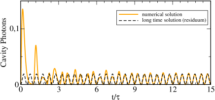
Figure 4: Comparison between numerics (orange curve) and long time solution determined by the residuum contribution only (black curve) for an initially excited TLS $c_{e}(0)=1$ and $\kappa/\gamma=2$. After several $\tau$, the analytical long time solution and the numerics coincide.

We now need to find a delay time $\tau$ in a way, that for $\pm i\gamma$, this equation is valid. As it turns out, the corresponding singularity condition can be matched for the following two cases:

$$(i)\exp(i\gamma\tau)=\exp(i\omega_{0}\tau)=1$$ (17)

$$(ii)\exp(-i\gamma\tau)=\exp(i\omega_{0}\tau)=1.$$ (18)

In order to satisfy these conditions we observe that we can freely choose the delay time with respect to the coupling strength by adjusting the length $L$ between cavity and mirror accordingly. For instance, if we choose $\gamma\tau=2\pi m$ and at the same time tune the resonance frequency such that $\omega_{0}\tau=2\pi l$, where $l,m$ are integer numbers, then the conditions $(i)$ and $(ii)$ are satisfied. (Note that there are also three other obvious constraints on $\tau$ and $\gamma$ to satisfy the conditions $(i)$ or $(ii)$ but they are not discussed below.) As a result we achieve a purely coherent asymptotic solution with a minimum of dephasing and a maximum amplitude, corresponding to the fact that the pole does not contain any decaying term. Indeed, we derive the following expression for the asymptotic behaviour of the photon density inside the cavity

$$c^{(i)}_{g}(t)=\frac{1}{2\pi i}\oint\text{d}s\ c_{g}(s)\ e^{st}\approx\sum_{\text{Poles}}\text{Res}\left[c_{g}(s)e^{st}\right]\,\,\,\,$$

$$= \sum_{\pm}\underset{s\rightarrow\pm i\gamma}{\text{lim}}\frac{(s\pm i\gamma)\exp[s2n\pi/\gamma]\ i\gamma}{(s+i\gamma)(s-i\gamma)+\kappa s\left(1-\exp[-s2m\pi/\gamma]\right)}.$$

Using now L’Hôpital’s rule and taking the limits $s\rightarrow\pm i\gamma$, the solution for $c_{g}(t)$ reads

$$c_{g}(t)=\frac{i\sin[\gamma t]}{1+\kappa m\pi/\gamma}.$$ (20)

In Fig. 4, the numerical solution and the analytical long time solution is plotted for $\tau=2\pi/\gamma$ (i.e. when $m=1$) up to several $\tau$. The agreement is excellent with the long time solution accurately recovering the amplitude and the oscillation frequency of the numerical solution. Interestingly, for $\kappa=0$, we recover the Jaynes-Cummings solution as in Eq. (10) with $\kappa=0$. In contrast to Eq. (10), we see, however, that the cavity loss does not modify the frequency of vacuum Rabi oscillations, which is now equal to the coupling strength $\gamma$, and only damps the corresponding amplitude. In this context, we discover a maximum amplitude for the feedback effect via this proposed mechanism. It is seen that Eq.(20) yields the following amplitude of the quantum feedback induced Rabi oscillations for $\tau=2\pi/\gamma$: $1/(1+\kappa\pi/\gamma)^{2}$. Therefore with $\kappa=2\gamma$, the maximum amplitude is approximately $0.02$ in correspondence with Fig. 4, which is 15% of the maximum photon amplitude in the first time interval $[0,\tau]$. With these results at hand we can now also answer the questions raised above:
(I) The effect of stabilized Rabi oscillations in the long time limit depends strongly on the chosen time delay $\tau$, which has to be chosen such to satisfy one of the conditions (17), (18) that lead to asymptotically undamped Rabi oscillations. Furthermore, the factor $\exp[i\omega_{0}\tau]$ plays a crucial role to decide whether quantum feedback leads to a stabilized Rabi oscillation or to a damped feedback situation. However, the effect depends only quantitatively (rather than qualitatively) on the cavity loss $\kappa$ and coupling strength $\gamma$, besides the obvious restriction that both of them are unequal to zero.
(II) For a given ratio between the coupling strength and the cavity loss, $x=\kappa/\gamma$, there is a maximum amplitude which is given for the above case by $(1+x\pi)^{-2}$.

II.4 Photon-Path Representation

To give an intuitive explanation for this effect of recovered Rabi oscillations in the weak coupling limit, we visualize the resulting cavity dynamics in the framework of the photon-path representation Alber et al. (2013); Stampfer et al. (2005). For this purpose we rewrite the system of equations of motion (7), (8) in the Laplace domain as:

$$\begin{pmatrix}c_{e}(0)\\ c_{g}(0)\end{pmatrix} = s\left[1-\mathbb{L}\right]\begin{pmatrix}c_{e}(s)\\ c_{g}(s)\end{pmatrix},$$ (21)

with the scattering matrix:

$$\mathbb{L}=\begin{pmatrix}0&i\frac{\gamma}{s}\\ i\frac{\gamma}{s}&-\frac{\kappa}{s}\left(e^{-\tau s}-1\right)\\ \end{pmatrix}.$$ (22)

Assuming that there is an inverse to that matrix and using the Neumann expansion, we get for $||\mathbb{L}||<1$:

$$\begin{pmatrix}c_{e}(s)\\ c_{g}(s)\end{pmatrix} = \frac{1}{s}\sum_{n=0}^{\infty}\mathbb{L}^{n}\begin{pmatrix}c_{e}(0)\\ c_{g}(0)\end{pmatrix}$$

$$= \sum_{n=0}^{\infty}\left[\frac{(i\gamma)^{n}}{s^{n+1}}\begin{pmatrix}0&1\\ 1&\frac{\kappa}{i\gamma}(e^{-\tau s}-1)\end{pmatrix}^{n}\right]\begin{pmatrix}c_{e}(0)\\ c_{g}(0)\end{pmatrix}$$

Now, the dynamics is written in a very complicated manner but in a way that the photon path (represented by scattering processes due to $\mathbb{L}$) becomes visible. With this expansion, one can represent the dynamics as a series of single scattering events by multiple application of the matrix, which swap the excitation from $c_{e}$ to $c_{g}$ and includes the cavity loss and the gain from the feedback. This becomes especially apparent, when writing down the single terms of the Laplace transform and then transforming them back into the time domain. In particular for the ground state probability such an expansion reads (terms up to $t^{3}$ are kept only):

$$c_{g}(t)=\dfrac{(i\gamma)}{1!}-\dfrac{(i\gamma)\kappa}{2!}t^{2}+\dfrac{(i\gamma)^{3}}{3!}t^{3}+\dfrac{(i\gamma)\kappa^{2}}{3!}t^{3}+...$$

$$\dfrac{(i\gamma)\kappa}{2!}(t-\tau)^{2}\theta(t-\tau)\!-\!\dfrac{(2i\gamma)\kappa^{2}}{3!}(t-\tau)^{3}\theta(t-\tau)\!+\!\!...\,\,\,\,\,\,\,\,\,\,$$ (24)

From the structure of this expansion follows that undamped Rabi oscillations can be viewed as a result of an interference between incoming and outgoing photonic paths provided that $\tau=2\pi/\gamma$. In other words, the strong coupling feature is produced by a destructive interference effect of the photon paths at the point within the waveguide, where the tunneling event between cavity and waveguide takes place. This expansion explains furthermore that it takes a minimum time for this effect to unfold, since at least two dissipatively interacting waves need to be in the waveguide.

II.5 Strong coupling limit

To complete the picture, we investigate the proposed feedback mechanism via a quasi-continuum in the strong coupling limit.

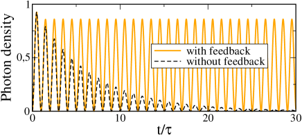
Figure 5: Fast stabilization of Rabi oscillations of the cavity photon number in the strong coupling limit $\gamma=20\kappa$ after only one roundtrip $\tau$, when the feedback from the waveguide is present (orange curve). Initially, the excitation is stored in the TLS ($c_{e}(0)=1$).

In Fig. 5, the dynamics with and without feedback is plotted for a a coupling strength $\gamma=20\kappa$. Clearly, Rabi oscillations are visible with and without feedback. If no feedback is present, however, the amplitude of the Rabi oscillations are damped fast without changing the frequency. With a feedback and a chosen delay time of $\tau=\pi/(2\gamma)$, on the other hand, the amplitude loss is stopped at very early times already: Already after one roundtrip the amplitude stays constant for all times, if no other loss mechanism inside or between mirror and cavity is present. We explain the acceleration of the stabilization feature by the fact, that for the strong coupling regime the in- and outgoing photons already interfere efficiently after one roundtrip. In contrast, in the weak coupling limit the in- and out tunneling does not overlap for the first three roundtrips and as a consequence inteference takes place at longer times only. If we choose a larger roundtrip time $\tau$, also in the strong coupling regime, a higher number of roundtrips $(n\tau)$ is necessary to reach the point of stabilized Rabi oscillations.

III Conclusion and outlook

We have discussed an approach to stabilize single-emitter cQED via a quantum feedback mechanism induced by an external mirror. Our analytical solution shows that depending on the chosen parameters an intrinsic limit of the feedback effects exists. For a system initially in the weak coupling regime (before the feedback modifies the system dynamics) we demonstrate that the quantum feedback can at most recover approximately 15% of the maximum cavity occupancy in the first time interval. Our analytic calculations demonstrate furthermore that the quantum feedback induced Rabi oscillations are indeed coherent and follow a typical differential delay equation with an appropriate inhomogeneity to drive the system into the strong coupling regime. Our results extend the set of exact analytical solutions in the field of coherent atom cQED and form a starting point to establish a framework for a theoretical description of coherent quantum feedback.

We would like to thank N. Naumann and S. Hein for helpful discussions. We acknowledge support from Deutsche Forschungsgemeinschaft through SFB 910 “Control of self-organizing nonlinear systems”. D.K. and S.R. are supported by the Austrian Science Fund (FWF) through project No. F49-P10 (SFB NextLite). AC acknowledges gratefully support from Alexander-von-Humboldt foundation through the Feodor-Lynen program.

References

- Hennessy et al. (2007) K. Hennessy, A. Badolato, M. Winger, D. Gerace, M. Atature, S. Gulde, S. Falt, E. L. Hu, and A. Imamoglu, Nature 445, 896 (2007).
- McKeever et al. (2003) J. McKeever, A. Boca, A. D. Boozer, J. R. Buck, and H. Kimble, Nature 425, 268 (2003).
- Putz et al. (2014) S. Putz, D. O. Krimer, R. Amsüss, A. Valookaran, T. Nöbauer, J. Schmiedmayer, S. Rotter, and J. Majer, Nat. Phys. 10 (2014).
- Krimer et al. (2014a) D. O. Krimer, M. Liertzer, S. Rotter, and H. E. Türeci, Physical Review A 89, 033820 (2014a).
- Fink et al. (2008) J. Fink, M. Göppl, M. Baur, R. Bianchetti, P. Leek, A. Blais, and A. Wallraff, Nature 454, 315 (2008).
- Schuster et al. (2008) I. Schuster, A. Kubanek, A. Fuhrmanek, T. Puppe, P. Pinske, K. Murr, and G. Rempe, Nature Physics 4, 382 (2008).
- Chang et al. (2007) D. Chang, A. Sorenson, E. Demler, and M. Lukin, Nature Physics 3, 807 (2007).
- Nielsen and Chuang (2000) M. A. Nielsen and I. L. Chuang, Quantum Computation and Quantum Information (Cambridge University Press, Cambridge, 2000).
- Monroe (2002) C. Monroe, Nature 416, 238 (2002).
- Zoller et al. (2005) P. Zoller, T. Beth, D. Binosi, R. Blatt, H. Briegel, et al., Eur. Phys. J. D 36, 203 (2005).
- Zhou et al. (2012) X. Zhou, I. Dotsenko, B. Peaudecerf, T. Rybarczyk, C. Sayrin, S. Gleyzes, J. M. Raimond, M. Brune, and S. Haroche, Phys. Rev. Lett. 108, 243602 (2012).
- Wiseman and Milburn (2006) H. Wiseman and G. Milburn, Quantum Measurement and Control (Cambridge University Press, Oxford, 2006).
- Albert et al. (2011) F. Albert, C. Hopfmann, S. Reitzenstein, C. Schneider, et al., Nat.Commun. 2, 366 (2011).
- Kopylov et al. (2015) W. Kopylov, C. Emary, E. Schöll, and T. Brandes, New Journal of Physics 17, 013040 (2015).
- Grimsmo et al. (2014) A. Grimsmo, A. Parkins, and B. Skagerstam, New Journal of Physics 16, 065004 (2014).
- Strasberg et al. (2013) P. Strasberg, G. Schaller, T. Brandes, and M. Esposito, Physical Review E 88, 062107 (2013).
- Pyragas and Novičenko (2013) K. Pyragas and V. Novičenko, Physical Review E 88, 012903 (2013).
- Hein et al. (2014) S. M. Hein, F. Schulze, A. Carmele, and A. Knorr, Phys. Rev. Lett. 113, 027401 (2014).
- Schulze et al. (2014) F. Schulze, B. Lingnau, S. M. Hein, A. Carmele, E. Schöll, K. Lüdge, and A. Knorr, Physical Review A 89, 041801 (2014).
- Carmele et al. (2013) A. Carmele, J. Kabuss, F. Schulze, S. Reitzenstein, and A. Knorr, Phys. Rev. Lett. 110, 013601 (2013).
- Shor (1995) P. W. Shor, Phys. Rev. A 52, R2493 (1995).
- van Enk et al. (1997) S. J. van Enk, J. I. Cirac, and P. Zoller, Phys. Rev. Lett. 79, 5178 (1997).
- Walls and Milburn (2007) D. Walls and G. Milburn, Quantum Optics (Springer, Berlin Heidelberg, 2007).
- Laucht et al. (2011) A. Laucht, N. Hauke, A. Neumann, T. Günthner, F. Hofbauer, A. Mohtashami, K. Müller, G. Böhm, M. Bichler, M.-C. Amann, et al., Journal of Applied Physics 109, 102404 (pages 5) (2011).
- Berger et al. (2014) C. Berger, U. Huttner, M. Mootz, M. Kira, S. Koch, J.-S. Tempel, M. Aßmann, M. Bayer, A. Mintairov, and J. Merz, Physical review letters 113, 093902 (2014).
- Dorner and Zoller (2002) U. Dorner and P. Zoller, Phys. Rev. A 66, 023816 (2002).
- Cook and Milonni (1987) R. Cook and P. Milonni, Physical Review A 35, 5081 (1987).
- Gardiner and Zoller (1991) C. Gardiner and P. Zoller, Quantum Noise (Springer, Berlin Heidelberg New York, 1991).
- Krimer et al. (2014b) D. O. Krimer, S. Putz, J. Majer, and S. Rotter, Phys. Rev. A 90, 043852 (2014b).
- Alber et al. (2013) G. Alber, J. Z. Bernád, M. Stobińska, L. L. Sánchez-Soto, and G. Leuchs, Phys. Rev. A 88, 023825 (2013).
- Stampfer et al. (2005) C. Stampfer, S. Rotter, J. Burgdörfer, and L. Wirtz, Phys. Rev. E 72, 036223 (2005).