Non-parametric Bayesian Models of Response Function in Dynamic Image Sequences

Abstract

Estimation of response functions is an important task in dynamic medical imaging. This task arises for example in dynamic renal scintigraphy, where impulse response or retention functions are estimated, or in functional magnetic resonance imaging where hemodynamic response functions are required. These functions can not be observed directly and their estimation is complicated because the recorded images are subject to superposition of underlying signals. Therefore, the response functions are estimated via blind source separation and deconvolution. Performance of this algorithm heavily depends on the used models of the response functions. Response functions in real image sequences are rather complicated and finding a suitable parametric form is problematic. In this paper, we study estimation of the response functions using non-parametric Bayesian priors. These priors were designed to favor desirable properties of the functions, such as sparsity or smoothness. These assumptions are used within hierarchical priors of the blind source separation and deconvolution algorithm. Comparison of the resulting algorithms with these priors is performed on synthetic dataset as well as on real datasets from dynamic renal scintigraphy. It is shown that flexible non-parametric priors improve estimation of response functions in both cases. MATLAB implementation of the resulting algorithms is freely available for download.

1 Introduction

Computer analysis of dynamic image sequences offers an opportunity to obtain information about organ function without invasive intervention. A typical example is replacement of invasive blood sampling by computer analysis of dynamic images [1]. The unknown input function can be obtained by deconvolution of the organ time activity curve and organ response function. Typically, both the input function and the response functions are unknown. Moreover, the time-activity curves are also not directly observed since the recorded images are observed as superposition of multiple signals. The superposition arise e.g. from partial volume effect in dynamic positron emission tomography [2] or dynamic and functional magnetic resonance imaging [3] or from projection of the volume into planar dynamic scintigraphy [4]. Analysis of the dynamic image sequences thus require to separate the original sources (source images) and their weights over the time forming the time-activity curves (TACs). The TACs are then decomposed into input function and response functions. Success of the procedure is dependent on the model of the image sequence.

The common model for dynamic image sequences is the factor analysis model [5], which assume linear combination of the source images and TACs. Another common model is that TAC arise as a convolution of common input function and source specific kernel [6, 7]. The common input function is typically the original signal from the blood and the role of convolution kernels vary from application area: impulse response or retention function in dynamic renal scintigraphy [8] or hemodynamic response function in functional magnetic resonance imaging [9]. In this paper, we will refer to the source kernels as the response functions, however other interpretations are also possible.

Analysis of the dynamic image sequences can be done with supervision of experienced physician or technician, who follows recommended guidelines and uses medical knowledge. However, we aim at fully automated approach where the analysis fully depends on the used model. The most sensitive parameter of the analysis is the model of the response functions (i.e. the convolution kernels). Many parametric models of response functions has been proposed, including the exponential model [10] or piece-wise linear model [11, 12]. An obvious disadvantage of the approach is that the real response function may differ from the assumed parametric models. Therefore, more flexible class of models based on non-parametric ideas were proposed such as averaging over region [13], temporal regularization using finite impulse response filters [14], or free-form response functions using automatic relevance determination principle in [15].

In this paper, we will study the probabilistic models of response functions using Bayesian methodology within the general blind source separation model [16]. The Bayesian approach was chosen for its inference flexibility and for its ability to incorporate prior information of models [17, 18]. We will formulate the prior model for general blind source separation problem with deconvolution [15] where the hierarchical structure of the model allow us to study various versions of prior models of response functions. Specifically, we design different prior models of the response functions with more parameters then the number of points in the unknown response function. The challenge is to regularize the estimation procedure such that all parameters are estimated from the observed data. We will use the approximate Bayesian approach known as the Variational Bayes method [19]. The resulting algorithms are tested on synthetic as well as on real datasets.

2 Probabilistic Blind Source Separation with Deconvolution

In this Section, we introduce a model of dynamic image sequences. Estimation of the model parameters yields an algorithm for Blind Source Separation and Deconvolution. Prior models of all parameters except for the response functions are described here while the priors for the response functions will be studied in details in the next section.

2.1 Model of Observation

Each recorded image is stored as a column vector $\mathbf{d}_{t}\in\mathbf{R}^{p\times 1},t=1,\dots,n$, where $n$ is total number of recorded images. Each vector $\mathbf{d}_{t}$ is supposed to be an observation of a superposition of $r$ source images $\mathbf{a}_{k}\in\mathbf{R}^{p\times 1},k=1,\dots,r$, stored again columnwise. The source images are weighted by their specific activities in time $t$ denoted as $x_{1,t},\dots,x_{r,t}\equiv\overline{\mathbf{x}}_{t}\in\mathbf{R}^{1\times r}$. Formally,

$$\mathbf{d}_{t}=\mathbf{a}_{1}x_{1,t}+\mathbf{a}_{2}x_{2,t}+\dots+\mathbf{a}_{r}x_{r,t}+\mathbf{e}_{t}=A\overline{\mathbf{x}}_{t}^{T}+\mathbf{e}_{t},$$ (1)

where $\mathbf{e}_{t}$ is the noise of the observation, $A\in\mathbf{R}^{p\times r}$ is the matrix composed from source images as its columns $A=[\mathbf{a}_{1},\dots,\mathbf{a}_{r}]$, and symbol $()^{T}$ denotes transposition of a vector or a matrix in the whole paper. The equation (1) can be rewritten in the matrix form. Suppose the observation matrix $D=[\mathbf{d}_{1},\dots,\mathbf{d}_{n}]\in\mathbf{R}^{p\times r}$ and the matrix with TACs in its columns, $X=[\overline{\mathbf{x}}_{1}^{T},\dots,\overline{\mathbf{x}}_{n}^{T}]^{T}\in\mathbf{R}^{n\times r}$. Note that we will use the bar symbol, $\overline{\mathbf{x}}_{k}$, to distinguish the $k$th row of matrix $X$, while $\mathbf{x}_{k}$ will be used to denote the $k$the column. Then, the (1) can be rewritten into the matrix form as

$$D=AX^{T}+E.$$ (2)

The tracer dynamics in each compartment is commonly described as convolution of common input function, vector $\mathbf{b}\in\mathbf{R}^{n\times 1}$, and source specific response function (convolution kernel, mathematically), vector $\mathbf{u}_{k}\in\mathbf{R}^{n\times 1},k=1,\dots,r$ [11, 20, 10]. Using convolution assumption, each TAC can be rewritten as

$$\mathbf{x}_{k}=B\mathbf{u}_{k},\,\,\,\forall k=1,\dots,r,$$ (3)

where the matrix $B\in\mathbf{R}^{n\times n}$ is composed from elements of input function $\mathbf{b}$ as

$$B=\left(\begin{array}[]{cccc}b_{1}&0&0&0\\ b_{2}&b_{1}&0&0\\ \dots&b_{2}&b_{1}&0\\ b_{n}&\dots&b_{2}&b_{1}\end{array}\right).$$ (4)

Suppose the aggregation of response functions $U=[\mathbf{u}_{1},\dots,\mathbf{u}_{r}]\in\mathbf{R}^{n\times r}$. Then, $X=BU$ and the model (2) can be rewritten as

$$D=AU^{T}B^{T}+E.$$ (5)

The task of subsequent analysis is to estimate the matrices $A$ and $U$ and the vector $\mathbf{b}$ from the data matrix $D$.

2.1.1 Noise Model

We assume that the noise has homogeneous Gaussian distribution with zero mean and unknown precision parameter $\omega$, $e_{i,j}=\mathcal{N}_{e_{i,j}}(0,\omega^{-1})$. Then, the data model (2) can be rewritten as

$$f(D|A,X,\omega)=\prod_{t=1}^{n}\mathcal{N}_{\mathbf{d}_{t}}(A\overline{\mathbf{x}}_{t},\omega^{-1}I_{p}),$$ (6)

where symbol $\mathcal{N}$ denotes Gaussian distribution and $I_{p}$ is identity matrix of the size given in its subscript. Since all unknown parameters must have their prior distribution in the Variational Bayes methodology, the precision parameter $\omega$ has a conjugate prior in the form of the Gamma distribution

$$f(\omega)=\mathcal{G}_{\omega}(\vartheta_{0},\rho_{0}),$$ (7)

with chosen constants $\vartheta_{0},\rho_{0}$.

2.2 Probabilistic Model of Source Images

The only assumption on source images is that they are sparse, i.e. only some pixels of source images are non-zeros. The sparsity is achieved using prior model that favors sparse solution depending on data [21]. We will employ the automatic relevance determination (ARD) principle [22] based on joint estimation of the parameter of interest together with its unknown precision. Specifically, each pixel $a_{i,j}$ of each source image has Gaussian prior truncated to positive values (see Appendix A.1) with unknown precision parameter $\xi_{i,j}$ which is supposed to have conjugate Gamma prior as

$$f(a_{i,k}|\xi_{i,k})= t\mathcal{N}_{a_{i,j}}(0,\xi_{i,k}^{-1}),$$ (8)

$$f(\xi_{i,k})= \mathcal{G}_{\xi_{i,j}}(\phi_{0},\psi_{0}),$$ (9)

for $\forall i=1,\dots,p,\forall k=1,\ldots,r,$ and $\phi_{0},\psi_{0}$ are chosen constants. The precisions $\xi_{i,j}$ form the matrix $\Xi$ of the same size as $A$.

2.3 Probabilistic Model of Input Function

The input function $\mathbf{b}$ is assumed to be a positive vector; hence, it will be modeled as truncated Gaussian distribution to positive values with scaling parameter $\varsigma\in\mathbf{R}$ as

$$f(\mathbf{b}|\varsigma)= t\mathcal{N}(\mathbf{0}_{n,1},\varsigma^{-1}I_{n}),$$ (10)

$$f(\varsigma)= \mathcal{G}(\zeta_{0},\eta_{0}),$$ (11)

where $\mathbf{0}_{n,1}$ denotes zeros matrix of the given size and $\zeta_{0},\eta_{0}$ are chosen constants.

2.4 Models of Response Functions

Figure 1: Hierarchical model for blind source separation with deconvolution problem.

So far, we have formulated the prior models for source images $A$ and input function $\mathbf{b}$ from decomposition of the matrix $D$. The task of this paper is to propose and study prior models for response functions $U$ as illustrated in Figure 1. Different choices of the priors on the response functions have strong influence on the results of the analysis which will be studied in the next section.

3 Non-parametric Prior Models of Response Function

Figure 2: Example of theoretical shape of response function (by [11]), left, and corresponding real-world shape of convolution kernels, right.

Here, we will formulate several prior models of response functions. Our purpose is not to impose any parametric form as it was done, e.g., in [11, 10] but model response function as a free-form curve with only influence from their prior models. The motivation is demonstrated in Figure 2, where a common parametric model [11] is compared to an example of response function obtained from real data. While the basic form of the response function is correct, exact parametric form of the function would be very complex. Therefore, we prefer to estimate each point on the response function individually. However, this leads to overparametrization and poor estimates would result without regularization. All models in this Section introduce regularization of the non-parametric function via unknown covariance of the prior with hyperparameters.

3.1 Orthogonal Prior

The first prior model assumes that each response function $\mathbf{u}_{k},k=1,\dots,r$, is positive and each response function is weighted by its own precision relevance parameter $\upsilon_{k}\in\mathbf{R}$ which has a conjugate Gamma prior:

$$f(\mathbf{u}_{k}|\upsilon_{k})= t\mathcal{N}_{\mathbf{u}_{k}}\left(\mathbf{0}_{n,1},\upsilon_{k}^{-1}I_{n}\right),$$ (12)

$$f(\upsilon_{k})= \mathcal{G}_{\upsilon_{k}}(\alpha_{0},\beta_{0}),$$ (13)

for $\forall k=1,\ldots,r$ and where $\alpha_{0},\beta_{0}$ are chosen constants.

The precision parameters $\upsilon_{k}$ serves for suppression of weak response functions during iterative computation and therefore as parameters responsible for estimation of number of relevant sources.

3.2 Sparse Prior

The model with sparse response functions has been introduced in [15]. The key assumption of this model is that the response functions are most likely sparse which is modeled similarly as in case of source images, Section 2.2, using the ARD principle. Here, each element of response function $u_{k,j}$ has its relevance parameter $\upsilon_{k,j}$ which is supposed to be conjugate Gamma distributed. In vector notation, each response function $\mathbf{u}_{k}$ has its precision matrix $\Upsilon_{k}$ with precision parameters $\upsilon_{k,j}$ on its diagonal and zeros otherwise. Then

$$f(\mathbf{u}_{k}|\Upsilon_{k})= t\mathcal{N}_{\mathbf{u}_{k}}\left(\mathbf{0}_{n,1},\Upsilon_{k}^{-1}\right),$$ (14)

$$f(\upsilon_{k,j})= \mathcal{G}_{\upsilon_{k,j}}(\alpha_{0},\beta_{0}),\ \ \ \forall j=1,\ldots,n,$$ (15)

where $\alpha_{0},\beta_{0}$ are chosen constants.

The employed ARD principle should suppress the noisy parts of response functions which should leads to clearer response functions and subsequently to clearer TACs.

3.3 Sparse Differences Prior

Modeling of only sparsity in response functions could possibly leads to arbitrary solution such as very non-smooth curve. The model of differences in response functions allow us to formulate the model favoring smooth response functions which is biologically reasonable requirement. Let suppose the model of differences of response function $\mathbf{u}_{k}$, $\nabla\mathbf{u}_{k}$, where the difference matrix $\nabla$ is defined as

$$\nabla=\left(\begin{array}[]{cccc}1&-1&0&0\\ 0&1&\ddots&0\\ 0&0&\ddots&-1\\ 0&0&0&1\end{array}\right),$$ (16)

with ARD prior on each difference using precision parameter $\upsilon_{k,j}$ forming again precision matrix $\Upsilon_{k}$; however, with precisions of differences on its diagonal. Then, we can formulate this problem equally as

$$f(\nabla\mathbf{u}_{k}|\Upsilon_{k})=t\mathcal{N}_{\nabla\mathbf{u}_{k}}\left(\mathbf{0}_{n,1},\Upsilon_{k}^{-1}\right)\ \ \ \Longleftrightarrow\ \ \ f(\mathbf{u}_{k}|\Upsilon_{k})=t\mathcal{N}_{\mathbf{u}_{k}}\left(\mathbf{0}_{n,1},\nabla^{-1}\Upsilon_{k}^{-1}\nabla^{-T}\right),$$ (17)

where symbol $()^{-T}$ denotes transpose and inversion of matrix. The prior model is accompanied by prior model for precisions in the same way as in (15):

$$f(u_{k,j})=\mathcal{G}_{\upsilon_{k,j}}(\alpha_{0},\beta_{0}),\ \ \ \forall j=1,\ldots,n,$$ (18)

where $\alpha_{0},\beta_{0}$ are chosen constants.

3.4 Wishart Prior

So far, we have modeled only the first or the second diagonal of the precision matrix $\Upsilon_{k}$. Each of these approaches have its advantages which we would like to generalize into estimation of several diagonals of the prior covariance matrix. However, this is difficult to solve analytically. Instead, we note that it is possible to create the model for the full prior covariance matrix of the response functions as well as their mutual interactions. For this task, we use vectorized form of response functions denoted as $\mathbf{u}\in\mathbf{R}^{nr\times 1}$, $\mathbf{u}=\mathrm{vec}(U)=\left[\mathbf{u}{}_{1}^{T},\dots,\mathbf{u}{}_{r}^{T}\right]^{T}$. This rearranging allow us to model mutual correlation between response functions. The full covariance matrix $\Upsilon\in\mathbf{R}^{nr\times nr}$ can be modeled using Wishart distribution, see Appendix A.2, as

$$f(\mathbf{u}|\Upsilon)= t\mathcal{N}_{\mathbf{u}}\left(\mathbf{0}_{nr,1},\Upsilon^{-1}\right),$$ (19)

$$f(\Upsilon)= \mathcal{W}_{\Upsilon}\left(\alpha_{0}I_{nr},\beta_{0}\right),$$ (20)

with scalar prior parameters $\alpha_{0},\beta_{0}$.

The advantage of this parametrization is obvious, the full covariance matrix is estimated. The disadvantage is this model is that for estimation $nr$ parameters in vector $\mathbf{u}$, we need to estimate $n^{2}r^{2}$ additional parameters in covariance structure. The problem is regularized by the prior on $\Upsilon$, (20), which is relatively weak regularization with potential side effects. We try to suppress these side effects in the next section.

3.5 Wishart Prior with Localization

Figure 3: The used localization matrix $L$ for the first two diagonals. The black pixels denote ones and the white pixels denote zeros. This example is given for $n=15$ and $r=3$.

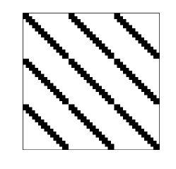
Since restriction of the covariance structure to several diagonals is infeasible in the considered dimensions, we apply an alternative approach known as localization. This techniques originates in data assimilation of atmospheric models [23]. The basic idea of the method is that the most information is localized on the first two diagonals of the matrix $\Upsilon$ and its sub-matrices. Hence, we can use Hadamard product, know also as element-wise product, of the original estimates $\Upsilon$ and localization matrix $L$ of the same size as the matrix $\Upsilon$. The localization matrix used in this paper for the first two diagonals is illustrated in Figure 3.

After localization, the model of response functions is the same as in Section 3.4, (19)–(20), however, the estimate of $\Upsilon$, ${\widehat{\Upsilon}}$, is replaced by

$${\widehat{\Upsilon}}_{new}={\widehat{\Upsilon}}\circ L,$$ (21)

where symbol $\circ$ denotes the Hadamard product. We will show that this localization is a soft version of smoothing of the Wishart model from Section 3.4; however, not so strict as modeling of differences in Section 3.3.

Theoretically, we could employ any conceivable localization as well as smoother version of localization using smooth transitions between ones and zeros; however, this is out of scope of this paper.

3.6 Variational Bayes Approximate Solution

The whole probabilistic model forming equations (6)–(7), (8)–(11), and selected response functions model from Sections 3.1–3.5. The probabilistic model is solved using Variational Bayes (VB) method [19]. Here, the solution is found in the form of probability densities of the same type of the priors. The shaping parameters of the posterior densities form a set of an implicit equations, Appendix B, which is typically analytically intractable and has to be solved iteratively.

1. Initialization:

   1. Set prior parameters $\alpha_{0},\beta_{0},\vartheta_{0},\rho_{0},\phi_{0},\psi_{0},\zeta_{0},\eta_{0}$.

   2. Set initial values for ${\widehat{A}},{\widehat{A^{T}A}},{\widehat{\Xi}},{\widehat{\mathbf{u}}},{\widehat{\mathbf{u}^{T}\mathbf{u}}},{\widehat{\Upsilon}},{\widehat{\mathbf{b}}},{\widehat{\mathbf{b}^{T}\mathbf{b}}},{\widehat{\varsigma}},{\widehat{\omega}}$.

   3. Set the initial number of sources $r_{max}$.

2. Iterate until convergence is reached using computation of shaping parameters from Appendix B:

   1. Source images $\mu_{\overline{\mathbf{a}}_{i}},\Sigma_{\overline{\mathbf{a}}_{i}}$ and their variances $\psi_{i},\phi_{i}$ $\forall i$ using (28)–(31).

   2. Response functions $\mu_{\mathbf{u}},\Sigma_{\mathbf{u}}$ and their hyper-parameters depending on version of the prior:

      1. RelRF: (37) and (38)–(39),

      2. SparseRF: (37) and (40)–(41),

      3. SparDifRF: (37) and (42)–(43),

      4. WishRF: (37) and (44)–(45),

      5. LocWishRF: (37) and (46)–(47).

   3. Input function $\mu_{\mathbf{b}},\Sigma_{\mathbf{b}}$ and its variance $\zeta,\eta$ using (32)–(34).

   4. Variance of noise $\vartheta,\rho$ using (35)–(36).

3. Report estimates of source images ${\widehat{A}}$, response functions ${\widehat{U}}$, and input function ${\widehat{\mathbf{b}}}$.

Algorithm 1

The algorithms are summarized in Algorithm 1. All prior parameters are set to $10^{-10}$ or $10^{+10}$ in order to obtained non-informative priors. The initial response functions are selected as pulses with different lengths with respect to cover the typical structures while the initial input function is selected as an exponential curve since the iterative solution could converge only to a local minimum [19].

4 Experiments and Discussion

We proposed five versions of model of non-parametric response functions within the model of probabilistic blind source separation model in Sections 3.1–3.5. The proposed algorithms are tested on simulated phantom study as well as on representative clinical data set from dynamic renal scintigraphy.

4.1 Synthetic Dataset

Figure 4: The results of the five studied methods on synthetic dataset (the first row). The red lines are generated data while the blue lines are estimated results from the respected methods.

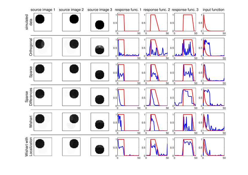
Performance of the proposed models of response functions is first studied on a synthetic dataset generated according to the model (5). The size of each image is $50\times 50$ pixels and the number of simulated time points is $n=50$. We simulate $3$ sources which are given in Figure 4, top row, using their source images and response functions together with generated input function $\mathbf{b}$ (top row, right). We generate homogeneous Gaussian noise with standard deviation $0.3$ of the signal strength.

The results of the five proposed models are given in Figure 4 in the row-wise schema. Note that all algorithms are capable to estimate the correct number of sources. It can be seen that all methods estimated the source images correctly. The main differences are in estimated response functions, the forth to the sixth columns, and estimated input function, the seventh column. Note that only the first prior, orthogonal, was not able to respect the sparse character of the modeled response functions, all other priors were able to do so. The visual results are accompanied by the corresponding mean square errors (MSE) summarized in Table 1. Here, the MSE is computed between the estimated response functions and their simulated values as well as between the estimated input functions and its simulated value for each method. The Wishart prior with localization outperforms the other ones in estimation of response functions while it is comparable with the sparse prior in estimation of input function.

Prior model of the response function	total MSE on $U$	MSE on $\mathbf{b}$
Orthogonal, Sec. 3.1	34.50	6.58
Sparse, Sec. 3.2	18.76	0.99
Sparse Differences, Sec. 3.3	22.84	8.03
Wishart, Sec. 3.4	30.33	3.43
Wishart with Localization, Sec. 3.5	9.26	1.19

Table 1: Computed mean square errors (MSE) from the simulated data.

4.1.1 Influence of Localization in Wishart Prior

Figure 5: Sensitivity study of MSE of estimated on the parameter $\alpha_{0}$ of the Wishart prior and the Wishart prior with localization.

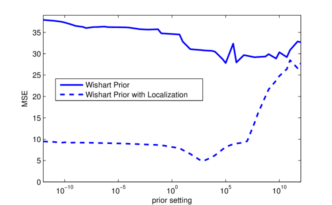
The effect of localization on the algorithm with the Wishart prior is illustrated studied in Figure 5 via sensitivity study of the prior parameter $\alpha_{0}$ on the resulting MSE of the response functions. The prior parameter $\beta_{0}$ is selected as $10^{-10}$ for all cases. For large values of $\alpha_{0}$ the results are comparable, however the localized version is improving with decreasing $\alpha_{0}$. For values of $\alpha_{0}<1$, the results of the localized version stabilize and become insensitive to the exact value of $\alpha_{0}$.

4.2 Datasets from Dynamic Renal Scintigraphy

The methods from Sections 3.1–3.5 were tested on real data from dynamic renal scintigraphy taken from online database. We illustrate the possible outcome of the method on two distinct datasets, numbers 84 and 42. Each dataset represent different behavior of the methods.

Both sequences consist of $50$ frames taken after $10$ seconds and both were preprocessed by selection region of the left kidney. The data are expected to contain three sources of activity: (i) parenchyma, the outer part of a kidney where the tracer is accumulated at the first, (ii) pelvis, the inner part of a kidney where the accumulation has physiological delay, and (iii) background tissues which is typically active at the beginning of the sequence. Since the noise in scintigraphy is Poisson distributed, the assumption of homogeneous Gaussian noise (6) can be achieved by asymptotic scaling known as the correspondence analysis [24] which transforms the original data $D_{orig}$ as

$$d_{ij}=\frac{d_{ij,orig}}{\sqrt{\sum_{i=1}^{p}d_{ij,orig}\sum_{j=1}^{n}d_{ij,orig}}}.$$ (22)

Figure 6: Estimated source images (columns 1–3), response functions (columns 4–6), and input functions (column 7) using priors: Orthogonal, Sparse, Sparse Differences, Wishart, Wishart with localization.

First, we applied the methods from Sections 3.1–3.5 on dataset number $84$ as a typical non-controversial case. The results are shown in Figure 6 using the estimated source images (columns 1–3), the estimated related response functions (columns 4–6), and the estimated input function (column 7). The results of all five methods are comparable with the main difference being in the smoothness or non-smoothness of the estimated response functions. This is most remarkable in the fifth column corresponding to the response functions of the pelvis. The sparse prior prefers sparse solution with many zeros, the sparse differences prior favors smooth solution (i.e. many differences being equal to zeros), while the Wishart prior models full covariance of response function where no smoothness is incorporated. The hypothetical compromise of all versions seems to be the Wishart prior with localization where the full covariance is modeled and subsequently localized. However, the differences in this case are relatively minor.

Figure 7: Estimated source images (columns 1–3), response functions (columns 4–6), and input functions (column 7) using priors: Orthogonal, Sparse, Sparse Differences, Wishart, Wishart with localization.

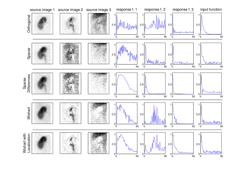
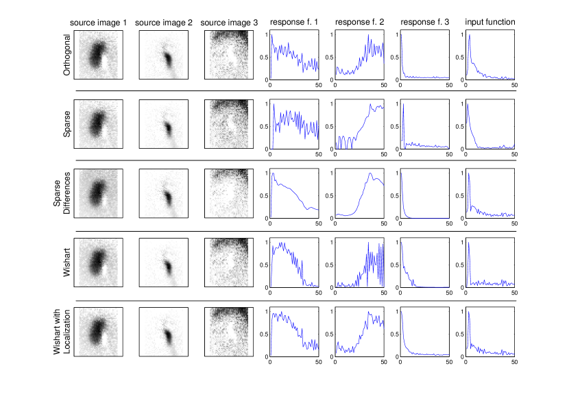
Second, we apply the methods 3.1–3.5 on dataset number $42$ where different methods yield more distinct results, see Figure 7. Note that the sparse and the sparse differences priors were not able to separate the pelvis which is mixed with the parenchyma in the first column while the orthogonal prior estimated the source images reasonably; however, the response functions of the parenchyma and the pelvis are clearly mixed. The Wishart-based priors, Wishart and Wishart with localization, were able to separate the parenchyma and the pelvis correctly together with meaningful estimates of their response functions. The main difference between the Wishart and the Wishart with localization priors is in smoothness. The estimated response functions from the Wishart prior with localization better matches the physiological expectations than the estimates from the Wishart model. In this case, the use of more complex prior models significantly outperform the simpler models.

Indeed, the analysis of the full database would be of interest in concrete application; however, it is not a goal of this paper.

5 Conclusion

A common model in functional analysis of dynamic image sequences assumes that the observed images arise from superposition of the original source images weighted by theirs time-activity curves. Each time-activity curve is assumed to be a result of common input function and source-specific response function, both unknown. Estimation of the model parameters yields an algorithm for blind source separation and deconvolution. The focus of this study is the prior model of the response functions while the models of the source images and the input function are the same. We propose five prior models of the response functions. The first three prior models are based on automatic relevance determination principle on the whole response functions, on each element of the response function, and on the differences between elements of the response functions, respectively. The forth model is based on full model of covariance matrix using Wishart distribution while the fifth model is based on the same prior; however, with additional localization within the deconvolution algorithm. The advantage of all five models is their flexibility in estimation of various shapes of response functions since we do not impose any parametric form of them. The formulated probabilistic models in the form of hierarchical priors are solved using the Variational Bayes methodology.

The performance of the proposed methods is tested on simulated dataset as well as on representative real datasets from dynamic renal scintigraphy. It is shown that the behaviors of the methods well correspond with their prior expectations. We conclude that the most complex model, i.e. the Wishart model with localization, provide also the most desirable results in the sense of mean square errors to the original simulated data as well as in sense of biologically meaningfulness of the results on the real datasets. Notably, the methods have no domain-specific assumptions; hence, they can be used in other task in dynamic medical imaging. The MATLAB implementation of all methods is available for download in http://www.utia.cz/bss_rf_priors/.

Appendix A Required Probability Distributions

A.1 Truncated Normal Distribution

Truncated normal distribution, denoted as $t\mathcal{N}$, of a scalar variable $x$ on interval $\left[a;b\right]$ is defined as

$$t\mathcal{N}(\mu,\sigma,\left[a,b\right])=\frac{\sqrt{2}\exp((x-\mu)^{2})}{\sqrt{\pi\sigma}(erf(\beta)-erf(\alpha))}\chi_{\left[a,b\right]}(x),$$ (23)

where $\alpha=\frac{a-\mu}{\sqrt{2\sigma}}$, $\beta=\frac{b-\mu}{\sqrt{2\sigma}}$, function $\chi_{\left[a,b\right]}(x)$ is a characteristic function of interval $\left[a,b\right]$ defined as $\chi_{\left[a,b\right]}(x)=1$ if $x\in\left[a,b\right]$ and $\chi_{\left[a,b\right]}(x)=0$ otherwise. $\mathrm{erf}()$ is the error function defined as $\mathrm{erf}(t)=\frac{2}{\sqrt{\pi}}\int_{0}^{t}e^{-u^{2}}\mathrm{d}u$.

The moments of truncated normal distribution are

$${\widehat{x}} =\mu-\sqrt{\sigma}\frac{\sqrt{2}[\exp(-\beta^{2})-\exp(-\alpha^{2})]}{\sqrt{\pi}(\mathrm{erf}(\beta)-\mathrm{erf}(\alpha))},$$ (24)

$${\widehat{x^{2}}} =\sigma+\mu\widehat{x}-\sqrt{\sigma}\frac{\sqrt{2}[b\exp(-\beta^{2})-a\exp(-\alpha^{2})]}{\sqrt{\pi}(\mathrm{erf}(\beta)-\mathrm{erf}(\alpha))}.$$ (25)

A.2 Wishart Distribution

Wishart distribution $\mathcal{W}$ of the positive-definite matrix $X\in\mathbf{R}^{p\times p}$ is defined as

$$\mathcal{W}_{p}(\Sigma,\nu)=|X|^{\frac{\nu-p-1}{2}}2^{-\frac{\nu p}{2}}|\Sigma|^{-\frac{\nu}{2}}\Gamma_{p}^{-1}\left(\frac{\nu}{2}\right)\exp\left(-\frac{1}{2}\mathrm{tr}\left(\Sigma^{-1}X\right)\right),$$ (26)

where $\Gamma_{p}\left(\frac{\nu}{2}\right)$ is the gamma function. The required moment is:

$$\widehat{X}= \nu\Sigma.$$ (27)

Appendix B Shaping Parameters of Posteriors

Shaping parameters of posterior distributions are given as:

$$\Sigma_{\overline{\mathbf{a}}_{i}}= \left({\widehat{\omega}}\sum_{j=1}^{n}({\widehat{\overline{\mathbf{x}}_{j}^{T}\overline{\mathbf{x}}_{j}}})+\mathrm{diag}({\widehat{\Xi_{i}}})\right)^{-1},$$ (28)

$$\mu_{\overline{\mathbf{a}}_{i}}= \Sigma_{\overline{\mathbf{a}}_{i}}{\widehat{\omega}}\sum_{j=1}^{n}({\widehat{\overline{\mathbf{x}}_{j}}}d_{i,j}),$$ (29)

$$\phi_{i}= \phi_{i,0}+\frac{1}{2}\mathbf{1}_{r,1},$$ (30)

$$\psi_{i}= \psi_{i,0}+\frac{1}{2}\mathrm{diag}\left({\widehat{\overline{\mathbf{a}}_{i}^{T}\overline{\mathbf{a}}_{i}}}\right),$$ (31)

$$\Sigma_{\mathbf{b}}= \left({\widehat{\varsigma}}I_{n}+{\widehat{\omega}}\sum_{i,j=1}^{r}({\widehat{\overline{\mathbf{a}}_{i}^{T}\overline{\mathbf{a}}_{j}}})\left(\sum_{k,l=0}^{n-1}\Delta_{k}^{T}\Delta_{l}{\widehat{u_{k+1,j}u_{l+1,i}}}\right)\right)^{-1},$$ (32)

$$\mu_{\mathbf{b}}= \Sigma_{\mathbf{b}}{\widehat{\omega}}\sum_{k=1}^{r}\left(\sum_{j=0}^{n-1}\Delta_{j}{\widehat{u_{j+1,k}}}\right)^{T}D^{T}{\widehat{\mathbf{a}_{k}}},$$ (33)

$$\zeta= \zeta_{0}+\frac{n}{2},\ \ \eta=\eta_{0}+\frac{1}{2}\mathrm{tr}\left({\widehat{\mathbf{b}^{T}\mathbf{b}}}\right),$$ (34)

$$\vartheta= \vartheta_{0}+\frac{np}{2},$$ (35)

$$\rho= \rho_{0}+\frac{1}{2}\mathrm{tr}\left(DD^{T}-{\widehat{A}}{\widehat{X}}^{T}D^{T}-D{\widehat{X}}{\widehat{A}}^{T}\right)+\frac{1}{2}\mathrm{tr}\left({\widehat{A^{T}A}}{\widehat{X^{T}X}}\right).$$ (36)

Here, ${\widehat{x}}$ denotes a moment of respective distribution, $\mathrm{tr}()$ denotes a trace of argument, $\mathrm{diag}()$ denotes a square matrix with argument vector on diagonal and zeros otherwise or a vector composed from diagonal element of argument matrix, $\mathbf{1}_{n,1}$ denotes the matrix of ones of dimension $n\times 1$, the auxiliary matrix $\Delta_{k}\in\mathbb{\mathbf{R}}^{n\times n}$ is defined as $(\Delta_{k})_{i,j}=\begin{cases}1,&\mathrm{if\,}i-j=k,\\ 0,&\mathrm{otherwise,}\end{cases}$, and standard moments of required probability distributions are given Appendix A.1 and A.2 and, e.g., in the appendix of [19].

The shaping parameters for response functions are given in following subsections while the parameter $\mu_{\mathbf{u}}$ is common for all methods as

$$\mu_{\mathbf{u}}=\Sigma_{\mathbf{u}}\left({\widehat{A^{T}A}}\otimes{\widehat{\omega}}{\widehat{B^{T}B}}\right)\mathrm{vec}\left({\widehat{B^{T}B}}^{-1}{\widehat{B}}^{T}D^{T}{\widehat{A}}{\widehat{A^{T}A}}^{-1}\right).$$ (37)

B.1 Shaping Parameters for Orthogonal Prior

$$\Sigma_{\mathbf{u}}= \left({\widehat{A^{T}A}}\otimes{\widehat{\omega}}{\widehat{B^{T}B}}+I_{n}\otimes{\widehat{\Upsilon}}\right)^{-1},$$ (38)

$$\alpha_{k}= \alpha_{k,0}+\frac{n}{2},\ \ \beta_{k}=\beta_{k,0}+\frac{1}{2}\mathrm{tr}\left({\mathbf{u}}_{k}{\mathbf{u}}_{k}^{T}\right),$$ (39)

B.2 Shaping Parameters for Sparse Prior

$$\Sigma_{\mathbf{u}}= \left({\widehat{A^{T}A}}\otimes{\widehat{\omega}}{\widehat{B^{T}B}}+\mathrm{diag}(\mathrm{vec}({\widehat{\Upsilon}}))\right)^{-1},$$ (40)

$$\alpha= \alpha_{0}+\frac{1}{2}\mathbf{1}_{nr,1},\ \ \beta=\beta_{0}+\frac{1}{2}\mathrm{diag}\left({\widehat{\mathbf{u}\mathbf{u}^{T}}}\right),$$ (41)

B.3 Shaping Parameters for Sparse Differences Prior

$$\Sigma_{\mathbf{u}}= \left({\widehat{A^{T}A}}\otimes{\widehat{\omega}}{\widehat{B^{T}B}}+(I_{r}\otimes\nabla){\widehat{\Upsilon}}(I_{r}\otimes\nabla^{T})\right)^{-1},$$ (42)

$$\alpha_{k}= \alpha_{k,0}+\mathbf{1}_{n,1}\frac{1}{2},\ \ \beta_{k}=\beta_{k,0}+\frac{1}{2}\mathrm{diag}\left(\nabla^{T}{\mathbf{u}}_{k}{\mathbf{u}}_{k}^{T}\nabla\right),$$ (43)

B.4 Shaping Parameters for Wishart Prior

$$\Sigma_{\mathbf{u}}= \left({\widehat{A^{T}A}}\otimes{\widehat{\omega}}{\widehat{B^{T}B}}+{\widehat{\Upsilon}}\right)^{-1},$$ (44)

$$\Sigma_{\Upsilon}= \left({\widehat{\mathbf{u}\mathbf{u}^{T}}}+(\alpha_{0}I_{nr})^{-1}\right)^{-1},\ \ \beta=\beta_{0}+1,$$ (45)

B.5 Shaping Parameters for Wishart Prior with Localization

$$\Sigma_{\mathbf{u}}= \left({\widehat{A^{T}A}}\otimes{\widehat{\omega}}{\widehat{B^{T}B}}+{\widehat{\Upsilon}}\circ L\right)^{-1},$$ (46)

$$\Sigma_{\Upsilon}= \left({\widehat{\mathbf{u}\mathbf{u}^{T}}}+(\alpha_{0}I_{nr})^{-1}\right)^{-1},\ \ \beta=\beta_{0}+1.$$ (47)

References

- [1] B. Lanz, C. Poitry-Yamate, R. Gruetter, Image-derived input function from the vena cava for 18F-FDG PET studies in rats and mice, Journal of Nuclear Medicine 55 (8) (2014) 1380–1388.
- [2] M. Margadán-Méndez, A. Juslin, S. Nesterov, K. Kalliokoski, J. Knuuti, U. Ruotsalainen, ICA based automatic segmentation of dynamic cardiac PET images., Information Technology in Biomedicine, IEEE Transactions on 14 (3) (2010) 795–802.
- [3] L. Chaari, T. Vincent, F. Forbes, M. Dojat, P. Ciuciu, Fast joint detection-estimation of evoked brain activity in event-related fMRI using a variational approach, Medical Imaging, IEEE Transactions on 32 (5) (2013) 821–837.
- [4] R. Di Paola, J. Bazin, F. Aubry, A. Aurengo, F. Cavailloles, J. Herry, E. Kahn, Handling of dynamic sequences in nuclear medicine, Nuclear Science, IEEE Transactions on 29 (4) (1982) 1310–1321.
- [5] A. Martel, A. Moody, S. Allder, G. Delay, P. Morgan, Extracting parametric images from dynamic contrast-enhanced mri studies of the brain using factor analysis, Medical image analysis 5 (1) (2001) 29–39.
- [6] J. Fleming, P. Kemp, A comparison of deconvolution and the Patlak-Rutland plot in renography analysis, Journal of Nuclear Medicine 40 (9) (1999) 1503.
- [7] T. Taxt, R. Jirik, C. B. Rygh, R. Gruner, M. Bartos, E. Andersen, F.-R. Curry, R. K. Reed, Single-channel blind estimation of arterial input function and tissue impulse response in dce-mri, Biomedical Engineering, IEEE Transactions on 59 (4) (2012) 1012–1021.
- [8] E. Durand, M. Blaufox, K. Britton, O. Carlsen, P. Cosgriff, E. Fine, J. Fleming, C. Nimmon, A. Piepsz, A. Prigent, et al., International Scientific Committee of Radionuclides in Nephrourology (ISCORN) consensus on renal transit time measurements, in: Seminars in nuclear medicine, Vol. 38, Elsevier, 2008, pp. 82–102.
- [9] M. A. Lindquist, J. Meng Loh, L. Y. Atlas, T. D. Wager, Modeling the hemodynamic response function in fmri: efficiency, bias and mis-modeling, Neuroimage 45 (1) (2009) S187–S198.
- [10] L. Chen, P. Choyke, T.-H. Chan, C.-Y. Chi, G. Wang, Y. Wang, Tissue-specific compartmental analysis for dynamic contrast-enhanced MR imaging of complex tumors, Medical Imaging, IEEE Transactions on 30 (12) (2011) 2044–2058.
- [11] A. Kuruc, W. Caldicott, S. Treves, Improved Deconvolution Technique for the Calculation of Renal Retention Functions., COMP. AND BIOMED. RES. 15 (1) (1982) 46–56.
- [12] O. Tichý, V. Šmídl, M. Šámal, Model-based extraction of input and organ functions in dynamic scintigraphic imaging, Computer Methods in Biomechanics and Biomedical Engineering: Imaging & Visualization(in print, doi:10.1080/21681163.2014.916229).
- [13] J. Kershaw, S. Abe, K. Kashikura, X. Zhang, I. Kanno, A bayesian approach to estimating the haemodynamic response function in event-related fmri, Neuroimage 11 (5) (2000) S474.
- [14] C. Goutte, F. A. Nielsen, L. K. Hansen, Modeling the hemodynamic response in fmri using smooth fir filters, Medical Imaging, IEEE Transactions on 19 (12) (2000) 1188–1201.
- [15] O. Tichý, V. Šmídl, Bayesian blind separation and deconvolution of dynamic image sequences using sparsity priors, Medical Imaging, IEEE Transaction on 34 (1) (2015) 1–9.
- [16] J. Miskin, Ensemble learning for independent component analysis, Ph.D. thesis, University of Cambridge (2000).
- [17] M. W. Woolrich, Bayesian inference in fmri, NeuroImage 62 (2) (2012) 801–810.
- [18] D. M. Steinberg, O. Pizarro, S. B. Williams, Hierarchical bayesian models for unsupervised scene understanding, Computer Vision and Image Understanding(in print, http://dx.doi.org/10.1016/j.cviu.2014.06.004).
- [19] V. Šmídl, A. Quinn, The Variational Bayes Method in Signal Processing, Springer, 2006.
- [20] B. Diffey, F. Hall, J. Corfield, The 99mTc-DTPA dynamic renal scan with deconvolution analysis, Journal of Nuclear Medicine 17 (5) (1976) 352.
- [21] M. Tipping, Sparse Bayesian learning and the relevance vector machine, The journal of machine learning research 1 (2001) 211–244.
- [22] C. Bishop, M. Tipping, Variational relevance vector machines, in: Proceedings of the 16th Conference on Uncertainty in Artificial Intelligence, 2000, pp. 46–53.
- [23] T. Hamill, J. Whitaker, C. Snyder, Distance-dependent filtering of background error covariance estimates in an ensemble kalman filter, Monthly Weather Review 129 (11) (2001) 2776–2790.
- [24] H. Benali, I. Buvat, F. Frouin, J. Bazin, R. Paola, A statistical model for the determination of the optimal metric in factor analysis of medical image sequences (FAMIS), Physics in medicine and biology 38 (1993) 1065.