BI-TP 2015/06

Critical point and scale setting in SU(3) plasma: An update

A. Francis^a, O. Kaczmarek^b, M. Laine^c, T. Neuhaus^d and H. Ohno^e,f

${}^{\mbox{\scriptsize a}}$Department of Physics and Astronomy, York University, 4700 Keele St.,
Toronto, ON M3J1P3, Canada

${}^{\mbox{\scriptsize b}}$Faculty of Physics, University of Bielefeld, 33501 Bielefeld, Germany

${}^{\mbox{\scriptsize c}}$Institute for Theoretical Physics, Albert Einstein Center, University of Bern,
Sidlerstrasse 5, 3012 Bern, Switzerland

${}^{\mbox{\scriptsize d}}$Institute for Advanced Simulation, Jülich Supercomputing Centre,
52425 Jülich, Germany

${}^{\mbox{\scriptsize e}}$Center for Computational Sciences, University of Tsukuba, Tsukuba,
Ibaraki 305-8577, Japan

${}^{\mbox{\scriptsize f}}$Physics Department, Brookhaven National Laboratory, Upton, NY 11973, USA

Abstract

We explore a method developed in statistical physics which has been argued to have exponentially small finite-volume effects, in order to determine the critical temperature $T_{\rm c}$ of pure SU(3) gauge theory close to the continuum limit. The method allows us to estimate the critical coupling $\beta_{c}$ of the Wilson action for temporal extents up to $N_{\tau}\sim 20$ with $\mathop{\raise 1.29167pt\hbox{$<$\kern-7.5pt\raise-4.73611pt\hbox{$\sim$}}}0.1\%$ uncertainties. Making use of the scale setting parameters $r_{0}$ and $\sqrt{t_{0}}$ in the same range of $\beta$-values, these results lead to the independent continuum extrapolations $T_{\rm c}r_{0}=0.7457(45)$ and $T_{\rm c}\sqrt{t_{0}}=0.2489(14)$, with the latter originating from a more convincing fit. Inserting a conversion of $r_{0}$ from literature (unfortunately with much larger errors) yields $T_{\rm c}/{\Lambda_{\overline{\mbox{\tiny\rm{MS}}}}}=1.24(10)$.

April 2015

1 Introduction

Even though light quarks play an essential role for the phenomenological understanding of heavy ion collision experiments it can be argued that, due to their large multiplicity in the initial state and their Bose-enhanced distribution functions in the plasma phase, gluons are the single most important degree of freedom influencing the formation and evolution of QCD matter. Gluons are also much easier to study with non-perturbative lattice methods than light quarks. Therefore studies of pure SU(3) gauge theory at high temperature continue to constitute an important laboratory system, both for developing numerical techniques and for gaining physics understanding on observables where a high precision is needed. Recent examples of topics studied include scale setting, renormalization, and methods for statistical error reduction (cf. e.g. refs. [2]–[6]). Our own interest stems from attempts to measure real-time observables such as transport coefficients [7]–[9], in which case theoretically well-founded methods [10] can probably be applied (if at all) only after the infinite volume and continuum limits have been reached with a high precision [11].

In the present contribution we use the pure SU(3) gauge theory as a test bench for studying finite-volume scaling in the vicinity of a first-order phase transition. Concretely, our primary goal is to determine the critical coupling $\beta_{c}$ for values of $N_{\tau}$ much larger than have been achieved before (here $N_{\tau}\equiv 1/(aT)$ is the number of lattice points in the periodic imaginary-time direction; $a$ is the lattice spacing; and $T$ is the temperature). Let us remark that values of $\beta_{c}$ as a function of $N_{\tau}$ have attracted recent interest as tests of semi-analytic models [12, 13], and indeed new high-precision values at large $N_{\tau}$ put the functional dependences predicted by these frameworks under tension [8].

The second focus point of our study is that of scale setting [14]. In particular, we consider two scales that have been frequently employed, denoted by $r_{0}$ [15] and $\sqrt{t_{0}}$ [16]. Neither of these scales has a direct physics interpretation; however they are relatively straightforward to measure and can in principle be related to physical quantities in a separate study. On the other hand, in the thermal context there is one directly physical quantity, the critical temperature $T_{\rm c}$, which would have certain advantages as a scale setting parameter, permitting for instance for an easy comparison of theories with different matter contents but with similar macroscopic properties (this assumes, of course, that all theories considered have a sharply defined transition point). Therefore, we make use of our results in order to obtain a largely independent estimate for $T_{\rm c}r_{0}$ [17] and a new estimate for $T_{\rm c}\sqrt{t_{0}}$. It should be acknowledged, however, that close to the continuum limit we also see indications of growing systematic uncertainties, particularly in case of $r_{0}$.

The plan of this note is the following. After introducing and testing the basic method of our study in sec. 2, we employ it in order to estimate the critical coupling $\beta_{c}$ as a function of $N_{\tau}$ in sec. 3. The issue of scale setting is addressed in sec. 4, and we conclude in sec. 5.

2 Method

The Wilson plaquette action,

$$S_{\mbox{\tiny\rm{W}}}\equiv\frac{\beta}{6}\sum_{x,\mu,\nu}{\rm Tr\,}(\mathbbm{1}-P_{\mu\nu})\;,$$ (1)

studied on an $N_{\tau}\times N_{s}^{3}$ lattice with periodic boundary conditions in all directions, has a global Z(3) symmetry that is broken at and above the transition point for $N_{\rm s}\to\infty$. We denote the location of the transition point by $\beta_{c}$. Theoretical arguments [18] and empirical evidence [19] suggest that this is a first order phase transition.

It has been shown through a study of $q$-state Potts models in three dimensions [20, 21] that even though most observables, such as susceptibilities, show powerlike finite-volume effects at a first-order transition point, there is a particular definition of a pseudocritical point for which finite-volume effects are exponentially suppressed. This is obtained if the “weights” of the phases with no degeneracy ($w_{c}$) and with $q$-fold degeneracy ($w_{d}$) are related through

$$q\,w_{c}=w_{d}\;.$$ (2)

The weight can be defined through the “volume” of the distribution of some observable which has a good overlap with the order parameter. More formally, the weight corresponds to the partition function associated with the phase considered.

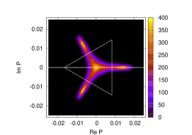
Figure 1: Left: Determination of the right-most minimum (open circle) from the distribution of $\mathop{\mbox{Re}}{P}$. Middle: The corresponding triangle separating the two phases, with the vertical line placed at the position of the open circle. Right: The resulting function $s(\beta)$ (cf. eq. (3)), permitting for an estimate of $\beta_{c}$ from the crossing of zero. The statistics of each data point is ${\mathcal{O}}(10^{5})$ sweeps; statistical errors are based on jackknife estimates.

For SU(3), a suitable observable is the Polyakov loop expectation value. Carrying out measurements in the vicinity of $\beta_{c}$, we define

$$s(\beta)\;\equiv\;\frac{3w_{c}-w_{d}}{3w_{c}+w_{d}}\;.$$ (3)

By construction $s(\beta)$ equals $+1$ deep in the confined and $-1$ deep in the deconfined phase. The critical point is obtained by interpolating to the location where $s(\beta_{c})=0$.

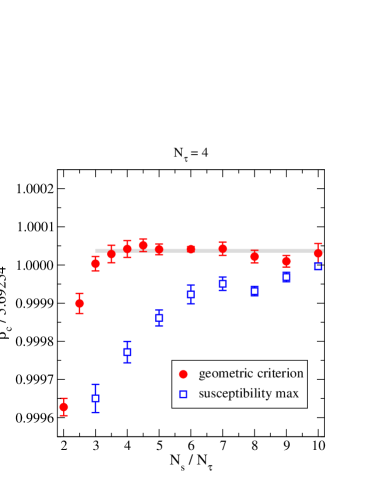
Figure 2: The pseudocritical couplings extracted from our method at $N_{\tau}=4$ (closed circles), normalized to the central value of the infinite-volume estimate $\beta_{c}=5.69254(24)$ from ref. [19]. We also compare with susceptibility maxima from ref. [22] (open squares). The grey band illustrates our infinite-volume extrapolation (constant fit to $N_{\rm s}/N_{\tau}>3$).

In order to implement the idea, we need to introduce a criterion for separating a distribution into contributions from different phases. In a finite volume, when the distributions overlap, the procedure is not unique. In this study, we define a separatrix by looking for a minimum in the distribution of $\mathop{\mbox{Re}}{P}$, where ${P}$ denotes the Polyakov loop (cf. fig. 1(left)). This minimum is employed for defining a triangle separating the two phases (cf. fig. 1(middle)). The resulting weights are the inputs for eq. (3); $\beta_{c}$ is obtained by a linear interpolation from points on both sides of the zero (cf. fig. 1(right)).

The results obtained with this procedure are shown in fig. 2 for $N_{\tau}=4$. They have been normalized to a classic value from ref. [19], and are compared with recent high-precision pseudocritical points extracted from Polyakov loop susceptibility maxima [22]. We conclude that for $N_{\rm s}>3N_{\tau}$, no finite-volume effects can be observed within our resolution ($\sim 0.005$%). For $N_{\rm s}<3N_{\tau}$, we expect $\beta_{c}$ to be slightly underestimated.

3 Results at finite lattice spacing

We carried out measurements for $4\leq N_{\tau}\leq 22$, increasing $N_{\tau}$ in steps of two. We computed on several volumes for ensembles with $N_{\tau}\leq 18$, verifying that volume dependence is below statistical uncertainties. Subsequently we fit the data at $N_{\rm s}>3N_{\tau}$ to a constant. Given the resources at our disposal we used a single spatial extent $N_{\rm s}=64$ for $N_{\tau}=20,22$. Here, minor finite-volume effects start to contaminate our results. However, based on fig. 2, we expect the effects from a simulation with $N_{\rm s}/N_{\tau}=64/22=2.9$ to be below the 0.01% level, thereby being much below statistical errors. In contrast, at the smallest $N_{\tau}$ where statistical errors are extremely small, we have artificially saturated the errors at a constant value $\sim 0.005\%$, corresponding to the expected uncertainty from finite-volume effects. Our final results at fixed $N_{\tau}$, together with previous estimates from the literature, are collected in table 1.

$N_{\tau}$	$\beta_{c}$ [19, 23]	$\beta_{c}$ [22]	$\beta_{c}$ [24]	$\beta_{c}$ [our value]	$N_{\rm s}$ used	$N_{\mbox{\scriptsize total}}$
4	5.69254(24)	5.692469(42)		5.69275(28)	14,…,40	83$\times 10^{6}$
5			5.8000(5)
6	5.8941(5)	5.89410(11)		5.89425(29)	20,…,40	28$\times 10^{6}$
8	6.0624(10)	6.06212(44)		6.06239(38)	28,32	4.2$\times 10^{6}$
10				6.20873(47)	32,…,56	15$\times 10^{6}$
12	6.3380(17)			6.33514(45)	40,…,72	21$\times 10^{6}$
14				6.4473(18)	48,56	12$\times 10^{6}$
16				6.5457(40)	64	2.5$\times 10^{6}$
18				6.6331(20)	56,64	3.6$\times 10^{6}$
20				6.7132(26)	64	4.0$\times 10^{6}$
22				6.7986(65)	64	5.9$\times 10^{6}$

Table 1: The infinite-volume critical points of SU(3) gauge theory according to various studies. $N_{\mbox{\scriptsize total}}$ indicates the total numbers of configurations (all volumes and values of $\beta$). Our data are based on constant fits to $N_{\rm s}>3N_{\tau}$ whenever several volumes are available. For $N_{\tau}=4,6$ we have artificially enlarged the errors to account for systematics related to exponentially small volume corrections (cf. the text).

4 Continuum extrapolations

In this section we convert the lattice-specific numbers of table 1 to values of $T_{\rm c}$ in physical units. In order to achieve this two different scale setting parameters are considered, $r_{0}$ and $\sqrt{t_{0}}$, with the latter leading to a noticeably better description of the thermal data (cf. sec. 4.2).

4.1 Scale $r_{0}$

$\beta$	$r_{0}/a$ [25]	$r_{0}/a$ [26]	$r_{0}/a$ [our value]	$N_{\tau}\times N_{\rm s}^{3}$	$N_{\mbox{\scriptsize conf}}$
5.7	2.922(9)
5.8	3.673(5)
5.95	4.898(12)
6.07	6.033(17)
6.2	7.380(26)
6.3			8.52(4)	$32\times 32^{3}$	216
6.3			8.51(2)	$32\times 48^{3}$	211
6.3			8.52(2)⋆	$32\times 64^{3}$	202
6.336			8.95(3)	$64\times 32^{3}$	220
6.4			9.80(3)	$36\times 36^{3}$	206
6.5			11.16(2)	$44\times 44^{3}$	202
6.57		12.18(10)⋆⋆
6.69		14.20(12)⋆⋆
6.81		16.54(12)⋆⋆
6.92		19.13(15)⋆⋆

Table 2: The results for $r_{0}/a$ that have been used in our analysis. For $\beta=6.3$ only the largest volume (indicated with an asterisk) has been included in subsequent fits. The values from ref. [26], marked with a double asterisk, do not come directly from $r_{0}$ but rather another scale $r_{c}$, which has been converted into $r_{0}$ through a continuum relation, whose systematic uncertainties are included in the errors.

The scale $r_{0}/a$ [15] has been measured as a function of $\beta$ in refs. [25, 26] (see ref. [27] and references therein for previous work). We complement these results by a new set of simulations, with parameter values and results listed in table 2. The measurements were separated by 500 heatbath-overrelaxation updates. A number of standard techniques for statistical error reduction [28, 29, 30] were implemented in order to obtain these results. The static potential is extracted from Wilson loops with an ansatz based on two exponentials. The distance appearing in the static potential is tree-level improved [26], and subsequently a B-spline interpolation is carried out in order to extract $r_{0}/a$ from its definition [15]. (Note that due to the several steps involved, measurements are costly and systematic errors are difficult to get fully under control, particularly at large $\beta$.)

$\beta$	$(t_{0}/a^{2})^{\rm Wilson}$	$(t_{0}/a^{2})^{\rm Wilson~{}imp.}$	$(t_{0}/a^{2})^{\rm Clover}$	$N_{\tau}\times N_{\rm s}^{3}$	$N_{\mbox{\scriptsize conf}}$
5.6923	0.6109(10)	0.8234(9)	1.0124(11)	$16\times 16^{3}$	455
5.6923	0.6103(7)	0.8229(6)	1.0119(7)	$16\times 24^{3}$	313
5.6923	0.6095(5)	0.8220(5)	1.0104(6)	$16\times 32^{3}$	248
5.6923	0.6010(4)	0.8226(4)	0.9905(4)	$24\times 32^{3}$	233
5.6923⋆	0.6097(3)	0.8223(3)	0.9800(4)	$32\times 32^{3}$	221
5.8941	1.9520(22)	2.0989(22)	2.2889(24)	$24\times 24^{3}$	465
6.0625	3.7129(39)	3.8507(39)	4.0626(41)	$32\times 32^{3}$	673
6.2083	5.9521(65)	6.0873(66)	6.3284(68)	$40\times 40^{3}$	476
6.3352	8.668(11)	8.802(11)	9.076(12)	$48\times 48^{3}$	315
6.4487	11.958(18)	12.091(18)	12.397(18)	$56\times 56^{3}$	254
6.5509	15.769(23)	15.901(23)	16.240(24)	$64\times 64^{3}$	305
6.7130	24.222(35)	24.355(35)	24.752(36)	$80\times 80^{3}$	250

Table 3: Our results for $t_{0}/a^{2}$. The $\beta$-values correspond approximately to those in table 1 (apart from $N_{\tau}=18,22$), with $N_{\tau}$ scaled up by a factor 4 in each case. For $\beta=5.6923$ only the largest volume (indicated with an asterisk) has been included in subsequent fits.

In order to permit for a subsequent interpolation, our data and older values [25, 26] are fit in the range $\beta\in(5.7,6.92)$ to a rational ansatz inspired by ref. [31]:

$$\ln\Bigl{(}\frac{r_{0}}{a}\Bigr{)}=\biggl{[}\frac{\beta}{12b_{0}}+\frac{b_{1}}{2b_{0}^{2}}\ln\Bigl{(}\frac{6b_{0}}{\beta}\Bigr{)}\biggr{]}\frac{1+c_{1}/\beta+c_{2}/\beta^{2}}{1+c_{3}/\beta+c_{4}/\beta^{2}}\;,$$ (4)

where $b_{0}\equiv 11/(4\pi)^{2}$ and $b_{1}\equiv 102/(4\pi)^{4}$. The fit parameters obtained read

$$c_{1}=-8.17273\;,\quad c_{2}=14.9600\;,\quad c_{3}=-3.95983\;,\quad c_{4}=-5.30334\;,\quad\chi^{2}/{\rm d.o.f.}=0.7\;.$$ (5)

Based on the above equation, we convert the results in table 1 to values of $r_{0}T_{\rm c}$: $r_{0}T_{\rm c}=(r_{0}/a)(\beta_{c})/N_{\tau}$. Subsequently we perform the extrapolation $(a/r_{0})^{2}\to 0$ using a fit quadratic in $(a/r_{0})^{2}$, illustrated in fig. 3(left), with the result

$$r_{0}T_{\rm c}=0.7457(45)\;,\quad\chi^{2}/{\rm d.o.f.}=6.7\;.$$ (6)

The error includes a rough estimate of systematic effects, encompassing the central values obtained by replacing the representation in eq. (4) through $\ln(r_{0}/a)=\sum_{n=0}^{3}a_{n}(\beta-6.25)^{n}$; by carrying out the continuum extrapolation with a cubic fit; and by omitting $\beta_{c}$ corresponding to $N_{\tau}=4$. The first method increases the central value ($T_{\rm c}{r_{0}}\simeq 0.7496$), the second and third decrease it ($T_{\rm c}{r_{0}}\simeq 0.7412,0.7424$, respectively). However, in the first case the quality of the continuum fit decreases further from the already poor one in eq. (6), whereas in the second case the scatter of the data in fig. 3(left) suggests that including too much freedom in the fit distorts the outcome. A possible reason for the poor description of the data close to the continuum limit could be that estimates of $r_{0}/a$ at $\beta>6.4$ are systematically on the low side (by $\sim{\mathcal{O}}(1$%)), but unfortunately we have not been able to confirm this suspicion.

The result in eq. (6) can be compared with $r_{0}T_{\rm c}\simeq 0.7470(7)$ obtained in ref. [8] based on peak positions of Polyakov loop susceptibilities (here only statistical errors were included), as well as with the earlier value $r_{0}T_{\rm c}=0.7498(50)$ [17].

Finally, we recall that e.g. the values $r_{0}{\Lambda_{\overline{\mbox{\tiny\rm{MS}}}}}=0.586(48)$ [26], $r_{0}{\Lambda_{\overline{\mbox{\tiny\rm{MS}}}}}=0.602(48)$ [32], $r_{0}{\Lambda_{\overline{\mbox{\tiny\rm{MS}}}}}=0.614(6)$ [33], and $r_{0}{\Lambda_{\overline{\mbox{\tiny\rm{MS}}}}}=0.637(32)$ [34] can be found in the literature (the third relies on the applicability of tadpole-improved lattice perturbation theory and the fourth of continuum perturbation theory at hadronic scales). Using the second value yields $T_{\rm c}/{\Lambda_{\overline{\mbox{\tiny\rm{MS}}}}}=1.24(10)$. Unfortunately the error is dominated by that in the relation of $r_{0}$ and ${\Lambda_{\overline{\mbox{\tiny\rm{MS}}}}}$, so our new result in eq. (6) does not help to improve on previous estimates.

4.2 Scale $\sqrt{t_{0}}$

The scale $\sqrt{t_{0}}$ is defined through the time that it takes for Wilson flow to adjust a chosen observable ($\equiv E$) to a predefined value [16]. We measured ${t_{0}}$ for a number of $\beta\simeq\beta_{c}$, as listed in table 1. To study possible systematic effects, we made use of three different implementations of $E$, based on the standard plaquette, tree-level improved, and clover discretizations, all of which are available within the DD-HMC package [35]. Like for $r_{0}$, the measurements were separated by 500 heatbath-overrelaxation updates; the volumes and the numbers of configurations used for measurements are shown in table 3.

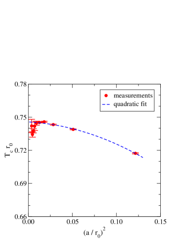
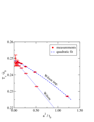
Figure 3: Left: Continuum extrapolation of $T_{\rm c}r_{0}$, based on the data in table 1 and the interpolation from eq. (5). Right: Analogous results for $T_{\rm c}\sqrt{t_{0}}$ from the “Wilson” (open circles) and “Wilson imp.” (closed circles) discretizations, interpolated according to eq. (7).

Given that the $\beta$ values of table 1 correspond to the critical point, a set of fixed physical volumes can be chosen by scaling the corresponding $N_{\tau}$ by a constant amount. Setting $N_{\rm s}=4N_{\tau}$ we ensure that the box size is $L=4/T_{\rm c}\simeq 5.3r_{0}$. For the smallest $\beta$ we have carried out test simulations also at larger volumes, finding consistent results apart from the “clover” discretization for which volume dependence on the 3% level is visible. For our final results we quote only those obtained with the two variants of the “Wilson” discretization that did not exhibit any volume dependence within statistical precision. Nevertheless systematic errors do grow with $\beta$, because a longer integration trajectory in $t$ is needed and because autocorrelation times tend to grow.

As before, we represent the data as in eq. (4) for the interpolation, only this time replacing $r_{0}\to\sqrt{t_{0}}$. The resulting parameters are (for the “Wilson imp.” discretization)

$$c_{1}=-10.2116\;,\quad c_{2}=25.6819\;,\quad c_{3}=-5.64462\;,\quad c_{4}=2.26845\;,\quad\chi^{2}/{\rm d.o.f.}=2.3\;.$$ (7)

With this interpolation the critical values in table 1 can be converted into $T_{\rm c}\sqrt{t_{0}}$; results are shown in fig. 3(right). A fit quadratic in $a^{2}/t_{0}$ yields

$$T_{\rm c}\sqrt{t_{0}}=0.2489(14)\;,\quad\chi^{2}/{\rm d.o.f.}=1.5\;.$$ (8)

The error bar here includes a rough estimate of systematic effects, encompassing the central values obtained by: (i) replacing “Wilson imp.” by “Wilson” or even the formerly excluded “clover” data; (ii) replacing the representation in eq. (4) through $\ln(\sqrt{t_{0}}/a)=\sum_{n=0}^{3}a_{n}(\beta-6.25)^{n}$; (iii) carrying out the continuum extrapolation with a cubic fit; (iv) omitting $\beta_{c}$ corresponding to $N_{\tau}=4$ from the fit. The biggest deviations ($T_{\rm c}\sqrt{t_{0}}\simeq 0.250$) result either from using “clover” data which we assume to suffer from finite-volume effects, or from method (ii) which leads to $\chi^{2}$ larger by more than an order of magnitude in eq. (8). (An analysis based on data for $t_{0}/a^{2}$ from previous literature can be found in ref. [9], is however subject to noticeably larger finite-volume effects than our current determination.)

Comparing eq. (8) with eq. (6), we extract $\sqrt{t_{0}}/r_{0}=0.3338(28)$, in perfect agreement with $\sqrt{t_{0}}/r_{0}=0.3343(21)$ from refs. [16, 36]. It is comforting to find a good agreement from a largely independent analysis.

5 Conclusions

In this note we have demonstrated that with modern resources and an opportune choice of an observable, the critical coupling $\beta_{c}$ of the Wilson plaquette action can be determined with $\mathop{\raise 1.29167pt\hbox{$<$\kern-7.5pt\raise-4.73611pt\hbox{$\sim$}}}0.1$% errors up to $N_{\tau}\sim 20$ (cf. table 1). Subsequently, the critical temperature $T_{\rm c}$ of pure SU(3) gauge theory could serve as a valid scale setting parameter for values of the Wilson coupling in the range $5.7\mathop{\raise 1.29167pt\hbox{$<$\kern-7.5pt\raise-4.73611pt\hbox{$\sim$}}}\beta\mathop{\raise 1.29167pt\hbox{$<$\kern-7.5pt\raise-4.73611pt\hbox{$\sim$}}}6.8$ (cf. table 1, from which the lattice spacing $a$ is obtained as $a=1/(N_{\tau}T_{\rm c})$ if we simulate at the $\beta_{c}$ corresponding to $N_{\tau}$). Unfortunately these values are not large enough for scale setting on the very fine lattices (for instance $N_{\tau}=48$, $\beta\simeq 7.8$) that are being used for studying transport observables close to the continuum limit [7]–[9]. Therefore “theoretical” quantities like $r_{0}$ and $\sqrt{t_{0}}$ continue to be needed as intermediate steps. On this point our study suggests that, with comparable numerical effort, employing $\sqrt{t_{0}}$ may yield more stable results than $r_{0}$, however being assured that systematic errors are below the percent level remains a challenge for $\beta>6.4$. If $\sqrt{t_{0}}$ is indeed used for scale setting, a conversion to $T_{\rm c}$ can be carried out through eq. (8): $\sqrt{t_{0}}T_{\rm c}=0.2489(14)$.

For various comparisons of lattice data with continuum perturbation theory, it would be very welcome to improve on our knowledge of $\sqrt{t_{0}}{\Lambda_{\overline{\mbox{\tiny\rm{MS}}}}}$, whose uncertainty is currently an order of magnitude larger than that of $\sqrt{t_{0}}T_{\rm c}$. Another issue worth further consideration is whether the method of sec. 2, which relied on the breaking of a discrete symmetry, could be generalized to the case of a continuous symmetry (such as a chiral symmetry).

References

- [1]
- [2] T. Umeda, S. Ejiri, S. Aoki, T. Hatsuda, K. Kanaya, Y. Maezawa and H. Ohno, Fixed Scale Approach to Equation of State in Lattice QCD, Phys. Rev. D 79 (2009) 051501 [0809.2842].
- [3] H.B. Meyer, High-Precision Thermodynamics and Hagedorn Density of States, Phys. Rev. D 80 (2009) 051502 [0905.4229].
- [4] Sz. Borsányi, G. Endrödi, Z. Fodor, S.D. Katz and K.K. Szabó, Precision SU(3) lattice thermodynamics for a large temperature range, JHEP 07 (2012) 056 [1204.6184].
- [5] M. Asakawa, T. Hatsuda, E. Itou, M. Kitazawa and H. Suzuki [FlowQCD Collaboration], Thermodynamics of SU(3) gauge theory from gradient flow on the lattice, Phys. Rev. D 90 (2014) 011501 [1312.7492].
- [6] L. Giusti and M. Pepe, Equation of state of a relativistic theory from a moving frame, Phys. Rev. Lett. 113 (2014) 031601 [1403.0360].
- [7] H.-T. Ding, A. Francis, O. Kaczmarek, F. Karsch, E. Laermann and W. Soeldner, Thermal dilepton rate and electrical conductivity: An analysis of vector current correlation functions in quenched lattice QCD, Phys. Rev. D 83 (2011) 034504 [1012.4963].
- [8] A. Francis, O. Kaczmarek, M. Laine, M. Müller, T. Neuhaus and H. Ohno, Towards the continuum limit in transport coefficient computations, PoS LATTICE 2013 (2014) 453 [1311.3759].
- [9] T. Neuhaus, Continuum study of heavy quark diffusion, to appear in the proceedings of 9th International Workshop on Critical Point and Onset of Deconfinement (17-21 November 2014, Bielefeld, Germany) [1504.07374].
- [10] G. Cuniberti, E. De Micheli and G.A. Viano, Reconstructing the thermal Green functions at real times from those at imaginary times, Commun. Math. Phys. 216 (2001) 59 [cond-mat/0109175].
- [11] Y. Burnier and M. Laine, Towards flavour diffusion coefficient and electrical conductivity without ultraviolet contamination, Eur. Phys. J. C 72 (2012) 1902 [1201.1994].
- [12] J. Langelage, S. Lottini and O. Philipsen, Centre symmetric 3d effective actions for thermal SU(N) Yang-Mills from strong coupling series, JHEP 02 (2011) 057 [Erratum-ibid. 07 (2011) 014] [1010.0951].
- [13] X. Cheng and E.T. Tomboulis, Critical couplings and string tensions via lattice matching of RG decimations, Phys. Rev. D 86 (2012) 074507 [1206.3816].
- [14] R. Sommer, Scale setting in lattice QCD, PoS LATTICE 2013 (2014) 015 [1401.3270].
- [15] R. Sommer, A New way to set the energy scale in lattice gauge theories and its applications to the static force and in SU(2) Yang-Mills theory, Nucl. Phys. B 411 (1994) 839 [hep-lat/9310022].
- [16] M. Lüscher, Properties and uses of the Wilson flow in lattice QCD, JHEP 08 (2010) 071 [Erratum-ibid. 03 (2014) 092] [1006.4518].
- [17] S. Necco, Universality and scaling behavior of RG gauge actions, Nucl. Phys. B 683 (2004) 137 [hep-lat/0309017].
- [18] B. Svetitsky and L.G. Yaffe, Critical Behavior at Finite Temperature Confinement Transitions, Nucl. Phys. B 210 (1982) 423.
- [19] G. Boyd, J. Engels, F. Karsch, E. Laermann, C. Legeland, M. Lütgemeier and B. Petersson, Thermodynamics of SU(3) lattice gauge theory, Nucl. Phys. B 469 (1996) 419 [hep-lat/9602007].
- [20] C. Borgs, R. Kotecký and S. Miracle-Solé, Finite size scaling for Potts models, J. Stat. Phys. 62 (1991) 529.
- [21] C. Borgs and W. Janke, A New method to determine first order transition points from finite size data, Phys. Rev. Lett. 68 (1992) 1738.
- [22] B.A. Berg and H. Wu, SU(3) deconfining phase transition with finite volume corrections due to a confined exterior, Phys. Rev. D 88 (2013) 074507 [1305.2975].
- [23] B. Beinlich, F. Karsch, E. Laermann and A. Peikert, String tension and thermodynamics with tree level and tadpole improved actions, Eur. Phys. J. C 6 (1999) 133 [hep-lat/9707023].
- [24] B. Lucini, M. Teper and U. Wenger, The High temperature phase transition in SU(N) gauge theories, JHEP 01 (2004) 061 [hep-lat/0307017].
- [25] M. Guagnelli, R. Sommer and H. Wittig [ALPHA Collaboration], Precision computation of a low-energy reference scale in quenched lattice QCD, Nucl. Phys. B 535 (1998) 389 [hep-lat/9806005].
- [26] S. Necco and R. Sommer, The heavy quark potential from short to intermediate distances, Nucl. Phys. B 622 (2002) 328 [hep-lat/0108008].
- [27] R.G. Edwards, U.M. Heller and T.R. Klassen, Accurate scale determinations for the Wilson gauge action, Nucl. Phys. B 517 (1998) 377 [hep-lat/9711003].
- [28] G. Parisi, R. Petronzio and F. Rapuano, A Measurement of the String Tension Near the Continuum Limit, Phys. Lett. B 128 (1983) 418.
- [29] P. de Forcrand and C. Roiesnel, Refined methods for measuring large distance correlations, Phys. Lett. B 151 (1985) 77.
- [30] M. Albanese et al. [APE Collaboration], Glueball Masses and String Tension in Lattice QCD, Phys. Lett. B 192 (1987) 163.
- [31] S. Dürr, Z. Fodor, C. Hoelbling and T. Kurth, Precision study of the SU(3) topological susceptibility in the continuum, JHEP 04 (2007) 055 [hep-lat/0612021].
- [32] S. Capitani, M. Lüscher, R. Sommer and H. Wittig [ALPHA Collaboration], Non-perturbative quark mass renormalization in quenched lattice QCD, Nucl. Phys. B 544 (1999) 669 [hep-lat/9810063].
- [33] M. Göckeler, R. Horsley, A.C. Irving, D. Pleiter, P.E.L. Rakow, G. Schierholz and H. Stüben, A Determination of the Lambda parameter from full lattice QCD, Phys. Rev. D 73 (2006) 014513 [hep-ph/0502212].
- [34] N. Brambilla, X. Garcia i Tormo, J. Soto and A. Vairo, Precision determination of from the QCD static energy, Phys. Rev. Lett. 105 (2010) 212001 [Erratum-ibid. 108 (2012) 269903] [1006.2066].
- [35] M. Lüscher, web page DD-HMC algorithm for two-flavour lattice QCD, http://luscher.web.cern.ch/luscher/DD-HMC/index.html.
- [36] M. Bruno and R. Sommer [ALPHA Collaboration], On the -dependence of gluonic observables, PoS LATTICE 2013 (2014) 321 [1311.5585].
- [37] M. Asakawa, T. Hatsuda, T. Iritani, E. Itou, M. Kitazawa and H. Suzuki, Accurate Determination of Reference Scales for Wilson Gauge Action from Yang–Mills Gradient Flow, 1503.06516.
- [38]