Numerical analysis of a robust free energy diminishing Finite Volume scheme for parabolic equations with gradient structure

Abstract.

We present a numerical method for approximating the solutions of degenerate parabolic equations with a formal gradient flow structure. The numerical method we propose preserves at the discrete level the formal gradient flow structure, allowing the use of some nonlinear test functions in the analysis. The existence of a solution to and the convergence of the scheme are proved under very general assumptions on the continuous problem (nonlinearities, anisotropy, heterogeneity) and on the mesh. Moreover, we provide numerical evidences of the efficiency and of the robustness of our approach.

1. Introduction

Many problems coming from physics (like e.g. porous media flows modeling [11, 10, 35]) or biology (like e.g. chemotaxis modeling [67]) lead to degenerate parabolic equations or systems. Many of these models can be interpreted as gradient flows in appropriate geometries. For instance, such variational structures were depicted for porous media flows [86, 70, 32], chemotaxis processes in biology [19], superconductivity [5, 4], or semiconductor devices modeling [84, 68] (this list is far from being complete).

Designing accurate numerical schemes for approximating their solutions is therefore a major issue. In the case of porous media flow models — used e.g. in oil-engineering, water resources management or nuclear waste repository management — the problems may moreover be highly anisotropic and heterogeneous. As an additional difficulty, the meshes are often prescribed by geological data, yielding non-conformal grids made of elements of various shapes. This situation can also be encountered in mesh adaptation procedures. Hence, the robustness of the method w.r.t. anisotropy and to the grid is an important quality criterion for a numerical method in view of practical applications.

In this contribution, we focus on the numerical approximation of a single nonlinear Fokker-Planck equation. Since it contains crucial difficulties arising in the applications, namely degeneracy and possibly strong anisotropy, the discretization of this nonlinear Fokker-Planck equation appears to be a keystone for the approximation of more complex problems.

1.1. Presentation of the continuous problem

Let $\Omega$ be a polyhedral connected open bounded subset of $\mathbb{R}^{d}$ ($d=2$ or $3$), and let ${t_{\rm f}}>0$ be a finite time horizon. In this contribution, we focus on the discretization of the model problem

(1) $$\begin{cases}\partial_{t}u-{\boldsymbol{\nabla}\cdot}\left(\eta(u){\boldsymbol{\Lambda}}\boldsymbol{\nabla}(p(u)+V)\right)=0&\text{ in }Q_{t_{\rm f}}:=\Omega\times(0,{t_{\rm f}}),\\ \left(\eta(u){\boldsymbol{\Lambda}}\boldsymbol{\nabla}(p(u)+V)\right)\cdot{\boldsymbol{n}}=0&\text{ on }\partial\Omega\times(0,{t_{\rm f}}),\\ u_{|_{t=0}}=u_{0}&\text{ in }\Omega,\end{cases}$$

which appears to be a keystone before discretizing more complex problems. We do the following assumptions on the data of the continuous problem (1).

• The function $\eta:\mathbb{R}_{+}\to\mathbb{R}_{+}$ is a continuous function such that $\eta(0)=0$, $\eta(u)>0$ if $u\neq 0$ and $\eta$ is non-decreasing on $\mathbb{R}_{+}$. The function $\eta$ is continuously extended on the whole $\mathbb{R}$ into an even function. It is called the mobility function in reference to the porous media flow context.

• The so-called (entropy) pressure function $p\in L^{1}_{\rm loc}(\mathbb{R}_{+})$ is absolutely continuous and increasing on $(0,+\infty)$ (i.e., $0<p^{\prime}\in L^{1}_{\rm loc}((0,+\infty))$), and satisfies $\lim_{u\to+\infty}p(u)=+\infty$. In the case where $p(0)=\lim_{u\searrow 0}p(u)$ is finite, the function $p$ is extended into an increasing absolutely continuous function $p:\mathbb{R}\to\mathbb{R}$ defined by

  (2) $$p(u)=2p(0)-p(-u),\qquad\forall u\leq 0.$$

  We denote by

  $${\mathcal{I}}_{p}=\begin{cases}\mathbb{R}_{+}^{\ast}&\text{ if }p(0)=-\infty,\\ \mathbb{R}&\text{ if }p(0)>-\infty.\\ \end{cases}$$

  and by ${\overline{{\mathcal{I}}}}_{p}$ its closure in $\mathbb{R}$. We additionally require that the function $\sqrt{\eta}p^{\prime}$ belongs to $L^{1}_{\rm loc}(\mathbb{R}_{+})$ (and is in particular integrable near $0$) and that $\lim_{u\searrow 0}\sqrt{\eta(u)}p(u)=0$.

• The tensor field ${\boldsymbol{\Lambda}}:\Omega\to(L^{\infty}(\mathbb{R}))^{d\times d}$ is such that ${\boldsymbol{\Lambda}}({\boldsymbol{x}})$ is symmetric for almost every ${\boldsymbol{x}}\in\Omega$. Moreover, we assume that there exist $\lambda_{\star}>0$ and $\lambda^{\star}\in[\lambda_{\star},+\infty)$ such that

  (3) $$\lambda_{\star}|{\bf v}|^{2}\leq{\boldsymbol{\Lambda}}({\boldsymbol{x}}){\bf v}\cdot{\bf v}\leq\lambda^{\star}|{\bf v}|^{2},\qquad\forall{\bf v}\in\mathbb{R}^{d},\;\text{for a.e. }{\boldsymbol{x}}\in\Omega.$$

  ${\boldsymbol{\Lambda}}$ is called the intrinsic permeability tensor field still in reference to the porous media flow context.

• The initial data $u_{0}$ is assumed to belong to $L^{1}(\Omega)$. Moreover, defining the convex function $\Gamma:{\overline{{\mathcal{I}}}}_{p}\to\mathbb{R}_{+}$ (called entropy function in the following) by

  (4) $$\Gamma(u)=\int_{1}^{u}(p(a)-p(1)){\rm d}a,\qquad\forall u\in{\mathcal{I}}_{p},$$

  we assume that the following positivity and finite entropy conditions are fulfilled:

  (5) $$u_{0}\geq 0\text{ a.e. in }\Omega,\qquad\int_{\Omega}u_{0}{\rm d}{\boldsymbol{x}}>0,\qquad\int_{\Omega}\Gamma(u_{0}){\rm d}{\boldsymbol{x}}<+\infty.$$

• The exterior potential $V:\Omega\to\mathbb{R}$ is Lipschitz continuous.

Throughout this paper, we adopt the convention

(6) $$\Gamma(u)=+\infty p(0)=-\infty u<0$$ if and .

In order to give a proper mathematical sense to the solution of (1), we need to introduce the function $\xi:\mathbb{R}_{+}\to\mathbb{R}_{+}$ defined by

(7) $$\xi(u)=\int_{0}^{u}\sqrt{\eta(a)}p^{\prime}(a){\rm d}a,\qquad\forall u\geq 0.$$

Note that $\xi$ is well defined since we assumed that $\sqrt{\eta}p^{\prime}$ belongs to $L^{1}_{\rm loc}(\mathbb{R}_{+})$. Moreover, in the case where $p(0)$ is finite, then the formula (7) can be extended to the whole $\mathbb{R}$, leading to an odd function. We additionally assume that the following relations between $\xi$, $\eta$ and $\Gamma$ hold:

• There exists $C>0$ such that

  (8) $$0\leq\xi(u)\leq C\left(1+\Gamma(u)\right),\qquad\forall u\in[0,+\infty).$$

  Moreover, we assume that

  (9) $$\frac{\Gamma(u)}{\eta(u)}\to+\infty\quad\text{ as }u\to+\infty,$$

  and that the function

  (10) $$\sqrt{\eta\circ\xi^{-1}}\;\text{is uniformly continuous on the range of $\xi$}.$$

Definition 1 (weak solution).

A measurable function $u$ is said to be a weak solution to problem (1) if

1. the functions $u$ and $\eta(u)$ belong to $L^{\infty}((0,{t_{\rm f}});L^{1}(\Omega))$;

2. the function $\xi(u)$ belongs to $L^{2}((0,{t_{\rm f}});H^{1}(\Omega))$;

3. for all function $\psi\in C^{\infty}_{c}({\overline{\Omega}}\times[0,{t_{\rm f}});\mathbb{R})$, one has

   (11) $$\iint_{Q_{t_{\rm f}}}u\partial_{t}\psi\,{\rm d}{\boldsymbol{x}}{\rm d}t+\int_{\Omega}u_{0}\psi(\cdot,0){\rm d}{\boldsymbol{x}}\\ -\iint_{Q_{t_{\rm f}}}\eta(u){\boldsymbol{\Lambda}}\boldsymbol{\nabla}V\cdot\boldsymbol{\nabla}\psi{\rm d}{\boldsymbol{x}}{\rm d}t-\iint_{Q_{t_{\rm f}}}{\boldsymbol{\Lambda}}\boldsymbol{\nabla}\xi(u)\cdot\sqrt{\eta(u)}\boldsymbol{\nabla}\psi{\rm d}{\boldsymbol{x}}{\rm d}t=0.$$

Following the seminal work of [2], there exists at least one weak solution $u$ to the problem (1). Denoting by

$$\phi(u)=\int_{0}^{u}\eta(a)p^{\prime}(a){\rm d}a,\qquad\forall u\in{\mathcal{I}}_{p},$$

the uniqueness of the solution (and even a $L^{1}$-contraction principle) is ensured as soon as $\eta\circ\phi^{-1}\in C^{0,1/2}$ (cf. [85], see also [7] for a slightly weaker condition in the case of a smooth domain $\Omega$). Moreover, $u$ belongs to $C([0,{t_{\rm f}}];L^{1}(\Omega))$ (cf. [31]) and $u(\cdot,t)\geq 0$ for all $t\in[0,{t_{\rm f}}]$ thanks to classical monotonicity arguments.

Remark 1.1.

Assumptions (${\bf A}1$)–(${\bf A}6$) formulated above deserve some comments.

• First of all, let us stress that Assumptions (${\bf A}1$)– (${\bf A}2$) and (${\bf A}6$) are satisfied if $\eta(u)=u$ and $p(u)=\log(u)$ as in the seminal paper of Jordan, Kinderlehrer, and Otto [65]. One can also deal with power like pressure functions $p(u)=u^{m-1}$, but only for $m>1$. Our study does not cover the case of the fast-diffusion equation $m<1$ with linear mobility function (see e.g. [86]) because of the technical assumption (${\bf A}6$).

• The most classical choice for the mobility function $\eta:\mathbb{R}_{+}\to\mathbb{R}_{+}$ is $\eta(u)=u$. In this case, the convection is linear. In this situation, the formal gradient flow structure highlighted in §1.2 can be made rigorous following the program proposed in [65, 86, 1, 3, 77] and many others. The gradient flow structure can also be made rigorous in the case where $\eta$ is concave (cf. [43]) and in the non-degenerate case $\eta(u)\geq\alpha>0$.

• One assumes in (${\bf A}1$) that $\eta$ is nondecreasing on $\mathbb{R}_{+}$. This assumption is natural in all the applications we have in mind. However, it is not mandatory in the proof and can be easily relaxed: it would have been sufficient to assume that there exists $\gamma>0$ such that

  $$\frac{\eta(a)+\eta(b)}{2}=\gamma\max_{s\in[a,b]}\eta(s),\qquad\forall[a,b]\subset\mathbb{R}.$$

  This relation is clearly satisfied with $\gamma=1/2$ when $\eta$ is nondecreasing.

• In Assumption (${\bf A}2)$, the condition $\lim_{u\to\infty}p(u)=+\infty$ ensures that

  $$\lim_{u\to\infty}\frac{\Gamma(u)}{u}=+\infty,$$

  where $\Gamma$ was defined in (${\bf A}4)$. Given a sequence $\left(u_{n}\right)_{n}\subset L^{1}(\Omega)$ with bounded entropy, i.e., such that $\int_{\Omega}\Gamma(u_{n}){\rm d}{\boldsymbol{x}}$ is bounded, then $\left(u_{n}\right)_{n}$ is uniformly equi-integrable thanks to the de La Vallée Poussin’s theorem [42]. Therefore, a sequence $\left(u_{n}\right)_{n}$ with bounded entropy relatively compact for the weak topology of $L^{1}(\Omega)$.

• Since the unique weak solution to the problem remains non-negative, the extension of $\eta$ and $p$ on the whole $\mathbb{R}$ could seem to be useless. However, in the case where $p(0)$ is finite, the non-negativity of the solution may not be preserved by the numerical method we propose. The extension of the functions $\eta$ and $p$ on $\mathbb{R}_{-}$ is then necessary.

• Only the regularity of the potential $V$ is prescribed by (${\bf A}5$). Confining potentials like e.g. $V({\boldsymbol{x}})=\frac{|{\boldsymbol{x}}-{\boldsymbol{x}}_{\star}|^{2}}{2}$ for some ${\boldsymbol{x}}_{\star}\in\Omega$, or gravitational potential $V({\boldsymbol{x}})=-\boldsymbol{g}\cdot{\boldsymbol{x}}$, where $\boldsymbol{g}$ is the (downward) gravity vector can be considered.

1.2. Formal gradient flow structure of the continuous problem

Let us highlight the (formal) gradient flow structure of the system (1). Following the path of [86, §1.3] (see also [84, 87]), the calculations carried out in this section are formal. They can be made rigorous under the non-degeneracy assumption $\eta(u)\geq\alpha>0$ for all $u\geq 0$.

Define the affine space

$$\mathfrak{M}=\left\{u:\Omega\to\mathbb{R}\;\left|\;\int_{\Omega}u({\boldsymbol{x}}){\rm d}{\boldsymbol{x}}=\int_{\Omega}u_{0}({\boldsymbol{x}}){\rm d}{\boldsymbol{x}}\right\}\right.$$

of the admissible states, called state space.

In order to define a Riemannian geometry on $\mathfrak{M}$, we need to introduce the tangent space $T_{u}\mathfrak{M}$, given by

$$T_{u}\mathfrak{M}=\left\{w:\Omega\to\mathbb{R}\;\left|\;\int_{\Omega}w({\boldsymbol{x}}){\rm d}{\boldsymbol{x}}=0\right\}\right..$$

We also need to define the metric tensor $\mathfrak{g}_{u}:T_{u}\mathfrak{M}\times T_{u}\mathfrak{M}\to\mathbb{R}$, which consists in a scalar product on $T_{u}\mathcal{M}$ (depending on the state $u$)

(12) $$\mathfrak{g}_{u}(w_{1},w_{2})=\int_{\Omega}\phi_{1}w_{2}\,{\rm d}{\boldsymbol{x}}=\int_{\Omega}w_{1}\phi_{2}{\rm d}{\boldsymbol{x}}=\int_{\Omega}\eta(u)\boldsymbol{\nabla}\phi_{1}\cdot{\boldsymbol{\Lambda}}\boldsymbol{\nabla}\phi_{2}\,{\rm d}{\boldsymbol{x}},$$

for all $w_{1},w_{2}\in T_{u}\mathfrak{M}$, where $\phi_{i}$ are defined via the elliptic problem

(13) $$\begin{cases}-{\boldsymbol{\nabla}\cdot}(\eta(u){\boldsymbol{\Lambda}}\boldsymbol{\nabla}\phi_{i})=w_{i}\text{ in }\Omega,\\[5.0pt] \eta(u){\boldsymbol{\Lambda}}\boldsymbol{\nabla}\phi_{i}\cdot{\boldsymbol{n}}=0\text{ on }\partial\Omega,\\[5.0pt] \displaystyle\int_{\Omega}\phi_{i}\,{\rm d}{\boldsymbol{x}}=0.\end{cases}$$

Note that $T_{u}\mathfrak{M}$ does not depend on $u$ (at least in the non-degenerate case), but the metric tensor $\mathfrak{g}_{u}(\cdot,\cdot)$ does. So we are not in a Hilbertian framework.

Define the free energy functional (cf. [64])

(14) $$\mathfrak{E}:\begin{cases}\mathfrak{M}\to\mathbb{R}\cup\{+\infty\}\\ \displaystyle u\mapsto\mathfrak{E}(u)=\int_{\Omega}\left(\Gamma(u({\boldsymbol{x}}))+u({\boldsymbol{x}})V({\boldsymbol{x}})\right){\rm d}{\boldsymbol{x}},\end{cases}$$

and the hydrostatic pressure function

$$\mathfrak{h}:\begin{cases}{\mathcal{I}}_{p}\times\Omega\to\mathbb{R}\\ (u,{\boldsymbol{x}})\mapsto\mathfrak{h}(u,{\boldsymbol{x}})=p(u)+V({\boldsymbol{x}})=D_{u}\mathfrak{E}(u).\end{cases}$$

Then given $w\in T_{u}\mathfrak{M}$, one has

(15) $$D_{u}\mathfrak{E}(u)\cdot w=\int_{\Omega}\mathfrak{h}(u({\boldsymbol{x}}),{\boldsymbol{x}})w({\boldsymbol{x}})\;{\rm d}{\boldsymbol{x}}=\int_{\Omega}\eta(u)\boldsymbol{\nabla}\mathfrak{h}(u,\cdot)\cdot{\boldsymbol{\Lambda}}\boldsymbol{\nabla}\phi\;{\rm d}{\boldsymbol{x}},$$

where $\phi$ is deduced from $w$ using the elliptic problem (13). Moreover, thanks to (12), one has

(16) $$\mathfrak{g}_{u}(\partial_{t}u,w)=\int_{\Omega}\partial_{t}u\,\phi\;{\rm d}{\boldsymbol{x}},\qquad\forall w\in T_{u}\mathfrak{M}.$$

In view of (15)–(16), the problem (1) is equivalent to

(17) $$\mathfrak{g}_{u}(\partial_{t}u,w)=-D_{u}\mathfrak{E}(u)\cdot w=-\mathfrak{g}_{u}(\boldsymbol{\nabla}_{u}\mathfrak{E}(u),w),\qquad\forall w\in T_{u}\mathfrak{M},$$

where the cotangent vector $D_{u}\mathfrak{E}(u)\in\left(T_{u}\mathfrak{M}\right)^{\ast}$ has been identified to the tangent vector $\boldsymbol{\nabla}_{u}\mathfrak{E}(u)\in T_{u}\mathfrak{M}$ thanks to Riesz theorem applied on $T_{u}\mathfrak{M}$ with the scalar product $\mathfrak{g}_{u}$. This relation can be rewritten as

(18) $$\partial_{t}u=-\boldsymbol{\nabla}_{u}\mathfrak{E}(u)={\boldsymbol{\nabla}\cdot}(\eta(u){\boldsymbol{\Lambda}}\boldsymbol{\nabla}\mathfrak{h}(u,\cdot))\quad\text{in }T_{u}\mathfrak{M},$$

justifying the gradient flow denomination.

Choosing $w=\partial_{t}u$ in (17) and using (18), we get that

$$\frac{{\rm d}}{{\rm d}t}\mathfrak{E}(u)=D_{u}\mathfrak{E}(u)\cdot\partial_{t}u=-D_{u}\mathfrak{E}(u)\cdot\boldsymbol{\nabla}_{u}\mathfrak{E}(u)=\int_{\Omega}\eta(u)\boldsymbol{\nabla}\mathfrak{h}(u,\cdot)\cdot{\boldsymbol{\Lambda}}\boldsymbol{\nabla}\mathfrak{h}(u,\cdot){\rm d}{\boldsymbol{x}}.$$

An integration w.r.t. time yields the classical energy/dissipation relation: $\forall t\in[0,{t_{\rm f}}]$,

(19) $$\mathfrak{E}(u(\cdot,t))-\mathfrak{E}(u_{0})\\ +\int_{0}^{t}\int_{\Omega}\eta(u({\boldsymbol{x}},\tau)){\boldsymbol{\Lambda}}({\boldsymbol{x}})\boldsymbol{\nabla}\mathfrak{h}(u({\boldsymbol{x}},\tau),{\boldsymbol{x}})\cdot\boldsymbol{\nabla}\mathfrak{h}(u({\boldsymbol{x}},\tau),{\boldsymbol{x}}){\rm d}{\boldsymbol{x}}{\rm d}\tau=0.$$

The fact that a physical problem has a gradient flow structure provides some informations concerning its evolution. The physical system aims at decreasing its free energy as fast a possible. As highlighted by (19), the whole energy decay corresponds to the dissipation. As a byproduct, the free energy is a Liapunov functional and the total dissipation (integrated w.r.t. time) is bounded by the free energy associated to the initial data. The variational structure was exploited for instance in [86, 21, 22, 93] to study the long-time asymptotic of the system.

1.3. Goal and positioning of the paper

The goal of this paper is to propose and analyse a numerical scheme that mimics at the discrete level the gradient flow structure highlighted in §1.2. Since the point of view adopted in our presentation concerning the gradient flow structure is formal, the rigorous numerical analysis of the scheme will rather rely on the well established theory of weak solutions in the sense of Definition 1. But as a byproduct of the formal gradient flow structure, the discrete free energy will decrease along time, yielding the non-linear stability of the scheme.

There are some existing numerical methods based on Eulerian coordinates (as the one proposed in this paper). This is for instance the case of monotone discretizations, that can be reinterpreted as Markov chains [81, 45], for which one can even prove a rigorous gradient flow structure. Classical ways to construct monotone discretizations in the isotropic setting ${\boldsymbol{\Lambda}}({\boldsymbol{x}})=\lambda({\boldsymbol{x}}){\bf I}_{d}$ are to use finite volumes schemes with two-points flux approximation (TPFA, see e.g. [51, 50]) or finite elements on Delaunay’s meshes (see e.g. [37]). An advanced second order in space finite volume method was proposed in [18] and discontinuous Galerkin schemes in [80, 79]. However, these approaches — as well as the finite difference scheme proposed in [78] — require strong assumptions on the mesh. Moreover, the extension to the anisotropic framework of TPFA finite volume scheme fails for consistency reasons (cf. [50]), while finite elements are no longer monotone on a prescribed mesh for general anisotropy tensors ${\boldsymbol{\Lambda}}$. In [61, 56], it appears that all the linear finite volume schemes (i.e., schemes leading to linear systems when linear equations are approximated) able to handle general grids and anisotropic tensors may loose at the discrete level the monotonicity of the continuous problem.

The monotonicity at the discrete level can be restored thanks to nonlinear corrections [27, 71, 30, 72]. Another approach consists in designing directly monotone nonlinear schemes (see, e.g., [66, 92, 75, 76, 44, 90]). However, the monotonicity of the method is not sufficient to ensure the decay of non-quadratic energies. Moreover, the available convergence proofs [44, 30] require some numerical assumptions involving the numerical solution itself. Finally, let us mention here the recent contribution [59] where linear monotone schemes are constructed on cartesian grids for possibly anisotropic tensors ${\boldsymbol{\Lambda}}$.

In the case where ${\boldsymbol{\Lambda}}={\bf I}_{d}$ and $\eta(u)=u$, the formal gradient flow structure can be made rigorous in the metric space

$$\mathcal{P}(\Omega):=\left\{u\in L^{2}(\Omega;\mathbb{R}_{+})\;\middle|\;\int_{\Omega}u{\rm d}{\boldsymbol{x}}=\int_{\Omega}u_{0}{\rm d}{\boldsymbol{x}}\right\}$$

endowed with the Wasserstein metric with quadratic cost function. Several approach were proposed in the last years for solving the JKO minimization scheme (cf. [65, 3]). This requires the computation of Wasserstein distances. If $d=1$, switching to Lagrangian coordinates is a natural choice that has been exploited for example in [69, 20, 82, 83]. The case $d\geq 2$ is more intricate. Methods based on a so-called entropic regularization [13, 88] of the transport plan appear to be costly, but very tractable. Another approach consists in solving the so-called Monge-Ampère equation in order to compute the optimal transport plan [15]. Let us finally mention the application [14] to the Wasserstein gradient flows of the CFD relaxation approach of Benamou and Brenier [12] to solve the Monge-Kantorovich problem.

Motivated by applications in the context of complex porous media flows where irregular grids are often prescribed by the geology, the scheme we propose was designed to be able to handle highly anisotropic and heterogeneous diffusion tensor ${\boldsymbol{\Lambda}}$ and very general grids (non-conformal grids, cells of various shapes). It relies on the recently developed Vertex Approximate Gradient (VAG) method [52, 54, 53, 26], but alternative versions can be inspired from most of the existing symmetric coercive methods for approximating the solutions of linear elliptic equations [61, 56]. Moreover, we want our scheme to mimic at the discrete level the gradient flow structure highlighted in §1.2. This ensures in particular the decay of the discrete counterpart of the free energy, and thus the nonlinear stability of the scheme.

A nonlinearly stable control volume finite elements (CVFE) scheme was proposed in our previous contribution [34] (see also [33]). The nonlinear CVFE scheme [34] is based on a suitable upwinding of the mobility. It is only first order accurate in space while linear CVFE schemes are second order accurate in space. Moreover, it appears in the numerical simulations presented in [34] that this nonlinear CVFE scheme lacks robustness with respect to anisotropy: its convergence is slow in particularly unfavorable situations.

The main goal of this paper is to propose a scheme that preserves some important features of the one introduced in [34] (possible use of some prescribed nonlinear test function, decay of the physically motivated energy, convergence proof for discretization parameters tending to $0$), without jeopardizing the accuracy of the scheme compared to the more classical approach based on formulations with Kirchhoff transforms (see for instance [57, 89, 58, 9]). Convincing numerical results are provided in §5 as an evidence of the efficiency of our approach. Two theorems are stated in §2.4 (and proved in §3 and §4) in order to ensure the following properties:

1. Theorem 2.3. At a fixed mesh, the scheme, that consists in a nonlinear system, admits (at least) one solution. This allows in particular to speak about the discrete solution provided by the scheme. Moreover, we take advantage of the gradient structure of the scheme for deriving some nonlinear stability estimates.

2. Theorem 2.4. Letting the discretization parameters tend to 0 (while controlling some regularity factors related to the discretization), the discrete solution converges in some appropriate sense towards the unique weak solution to the problem (1) in the sense of Definition 1.

Remark 1.2.

We only consider potential convection in the paper. A more general convection with speed ${\bf v}$ can be split into a potential part and a divergence free part:

$${\bf v}=-\nabla V+\nabla\times{\bf w}.$$

We suggest for instance to use classical (entropy stable) finite volume schemes (see for instance [74]) for the divergence free part combined with our method for the potential part.

2. Definition of the scheme and main results

As already mentioned, the scheme we propose is based on the so-called VAG scheme [52]. In §2.1, we state our assumptions on the spatial mesh and the time discretization of $(0,{t_{\rm f}})$. Then in §2.2, we define the nonlinear scheme we will study in this paper. The gradient flow structure of the discretized problem is highlighted in §2.3, where a variational interpretation is given to the scheme. Finally, in §2.4, we state the existence of discrete solutions to the scheme and their convergence towards the unique weak solution as the discretization parameters tend to $0$.

2.1. Discretization of $Q_{t_{\rm f}}$ and discrete functional spaces

2.1.1. Spatial discretization and discrete reconstruction operators

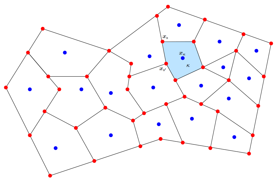
Following [53, 26], we consider generalized polyhedral discretizations of $\Omega$. Let $\mathcal{M}$ be the set of the cells, that are disjoint polyhedral open subsets of $\Omega$ such that $\bigcup_{\kappa\in\mathcal{M}}{\overline{\kappa}}={\overline{\Omega}}.$ Each cell $\kappa\in\mathcal{M}$ is assumed to be star-shaped with respect to its so-called center, denoted by ${\boldsymbol{x}}_{\kappa}$. We denote by $\mathcal{F}$ the set of the faces of the mesh, which are not assumed to be planar if $d=3$ (whence the term “generalized polyhedral”). We denote by $\mathcal{V}$ the set of the vertices of the mesh. We denote by ${\boldsymbol{x}}_{\rm s}\in{\overline{\Omega}}$ the location of the vertex ${\rm s}\in\mathcal{V}$. The sets $\mathcal{V}_{\kappa}$, $\mathcal{F}_{\kappa}$ and $\mathcal{V}_{\sigma}$ denote respectively the vertices and faces of a cell $\kappa$, and the vertices of a face $\sigma$. For any face $\sigma\in\mathcal{F}_{\kappa}$, one has $\mathcal{V}_{\sigma}\subset\mathcal{V}_{\kappa}$. Let $\mathcal{M}_{\rm s}$ denote the set of the cells sharing the vertex ${\rm s}$. The set of edges of the mesh (defined only if $d=3$) is denoted by $\mathcal{E}$ and $\mathcal{E}_{\sigma}$ denotes the set of edges of the face $\sigma\in\mathcal{F}$, while $\mathcal{E}_{\kappa}$ denotes the set of the edges of the cell $\kappa$. The set $\mathcal{V}_{\rm e}$ denotes the pair of vertices at the extremities of the edge ${\rm e}\in\mathcal{E}$. In the $3$-dimensional case, it is assumed that for each face $\sigma\in\mathcal{F}$, there exists a so-called “center” of the face ${\boldsymbol{x}}_{\sigma}$ such that

(20) $${\boldsymbol{x}}_{\sigma}=\sum_{{\rm s}\in\mathcal{V}_{\sigma}}\beta_{\sigma,{\rm s}}{\boldsymbol{x}}_{\rm s},\qquad\text{with }\quad\sum_{{\rm s}\in\mathcal{V}_{\sigma}}\beta_{\sigma,{\rm s}}=1,$$

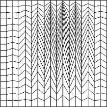
and $\beta_{\sigma,{\rm s}}\geq 0$ for all ${\rm s}\in\mathcal{V}_{\sigma}$. The face $\sigma$ is then assumed to match with the union of the triangles $T_{\sigma,{\rm e}}$ defined as by the face center ${\boldsymbol{x}}_{\sigma}$ and each of its edge ${\rm e}\in\mathcal{E}_{\sigma}$. A two-dimensional example of mesh $\mathcal{M}$ is drawn on figure 1.

The previous discretization is denoted by $\mathcal{D}$, and we define the discrete space

$$W_{\mathcal{D}}=\left\{{\boldsymbol{v}}=\left(v_{\kappa},v_{\rm s}\right)_{\kappa\in\mathcal{M},{\rm s}\in\mathcal{V}}\in\mathbb{R}^{\#\mathcal{M}+\#\mathcal{V}}\right\}.$$

In the $3$-dimensional case, we introduce for all $\sigma\in\mathcal{F}$ the operator $I_{\sigma}:W_{\mathcal{D}}\to\mathbb{R}$ defined by

$$I_{\sigma}({\boldsymbol{v}})=\sum_{{\rm s}\in\mathcal{V}_{\sigma}}\beta_{\sigma,{\rm s}}v_{\rm s},\qquad\forall{\boldsymbol{v}}\in W_{\mathcal{D}},$$

yielding a second order interpolation at ${\boldsymbol{x}}_{\sigma}$ thanks to the definition (20) of ${\boldsymbol{x}}_{\sigma}$.

Figure 1. The primal mesh $\mathcal{M}$ can be made of cells with various and general shapes. Degrees of freedom are located at the so-called cell center (blue dots) and at the so-called vertices (red dots).

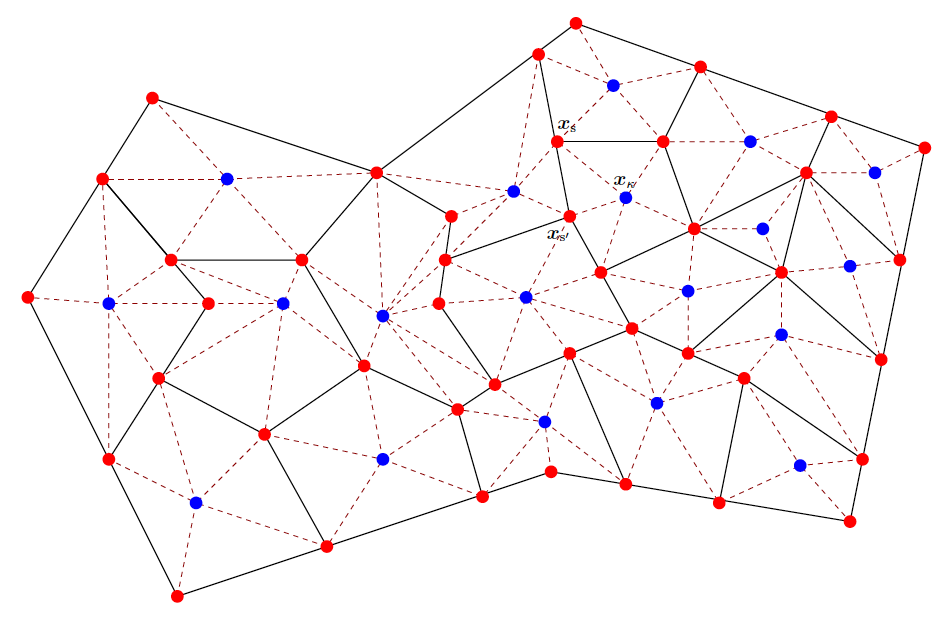
We introduce the simplicial submesh $\mathcal{T}$ (a two-dimensional illustration is provided on Figure 2) defined by

• $\mathcal{T}=\{T_{\kappa,\sigma},\kappa\in\mathcal{M},\sigma\in\mathcal{F}_{\kappa}\}$ in the two-dimensional case, where $T_{\kappa,\sigma}$ denotes the triangle whose vertices are ${\boldsymbol{x}}_{\kappa}$ and ${\boldsymbol{x}}_{\rm s}$ for ${\rm s}\in\mathcal{V}_{\sigma}$;

• $\mathcal{T}=\{T_{\kappa,\sigma,{\rm e}},\kappa\in\mathcal{M},\sigma\in\mathcal{F}_{\rm s},\,{\rm e}\in\mathcal{E}_{\sigma}\}$ in the three-dimensional case, where $T_{\kappa,\sigma,{\rm e}}$ denotes the tetrahedron whose vertices are ${\boldsymbol{x}}_{\kappa}$, ${\boldsymbol{x}}_{\sigma}$ and ${\boldsymbol{x}}_{\rm s}$ for ${\rm s}\in\mathcal{V}_{\rm e}$.

Figure 2. The simplicial submesh $\mathcal{T}$ is derived from the primal mesh $\mathcal{M}$ by decomposing the primal cells $\kappa\in\mathcal{M}$ into triangles if $d=2$ or tetrahedra if $d=3$. This construction is possible since $\kappa$ was assumed to be star-shaped with respect to a ball centered in ${\boldsymbol{x}}_{\kappa}$.

We define the regularity $\theta_{\mathcal{T}}$ of the simplicial mesh $\mathcal{T}$ by

(21) $$\theta_{\mathcal{T}}=\max_{T\in\mathcal{T}}\frac{h_{T}}{\rho_{T}},$$

where $h_{T}$ and $\rho_{T}$ respectively denote the diameter of $T$ and the insphere diameter of $T$. We denote by

(22) $$h_{\mathcal{T}}=\max_{T\in\mathcal{T}}h_{T}$$

the maximum diameter of the simplicial mesh. We also define the quantities $\ell_{\kappa}$ and $\ell_{\rm s}$ quantifying the number of vertices of the cell $\kappa$ and the number of neighboring cells for the vertex ${\rm s}$ respectively:

(23) $$\ell_{\kappa}=\#\mathcal{V}_{\kappa},\quad\ell_{\rm s}=\#\mathcal{M}_{\rm s},\quad\forall\kappa\in\mathcal{M},\;\forall{\rm s}\in\mathcal{V}.$$

This allows to introduce the quantity

(24) $$\ell_{\mathcal{D}}=\max\left(\max_{\beta\in\mathcal{M}\cup\mathcal{V}}\ell_{\beta},\max_{\kappa\in\mathcal{M}}\{\#\mathcal{F}_{\kappa}\}\right),$$

controlling the regularity of the general discretization $\mathcal{D}$ of $\Omega$.

Denoting by $H_{\mathcal{T}}\subset W^{1,\infty}(\Omega)$ the usual $\mathbb{P}_{1}$-finite element space on the simplicial mesh $\mathcal{T}$, we define the reconstruction operator $\pi_{\mathcal{T}}:W_{\mathcal{D}}\to H_{\mathcal{T}}$ by setting, for all ${\boldsymbol{v}}\in W_{\mathcal{D}}$ and all $({\rm s},\kappa,\sigma)\in\mathcal{V}\times\mathcal{M}\times\mathcal{F}$,

(25) $$\pi_{\mathcal{T}}{\boldsymbol{v}}({\boldsymbol{x}}_{\rm s})=v_{\rm s},\quad\pi_{\mathcal{T}}{\boldsymbol{v}}({\boldsymbol{x}}_{\kappa})=v_{\kappa},\quad\text{and}\quad\pi_{\mathcal{T}}{\boldsymbol{v}}({\boldsymbol{x}}_{\sigma})=I_{\sigma}({\boldsymbol{v}}).$$

This allows to define the operator $\boldsymbol{\nabla}_{\mathcal{T}}:W_{\mathcal{D}}\to(L^{\infty}(\Omega))^{d}$ by

(26) $$\boldsymbol{\nabla}_{\mathcal{T}}{\boldsymbol{v}}=\boldsymbol{\nabla}\pi_{\mathcal{T}}{\boldsymbol{v}},\qquad\forall{\boldsymbol{v}}\in W_{\mathcal{D}}.$$

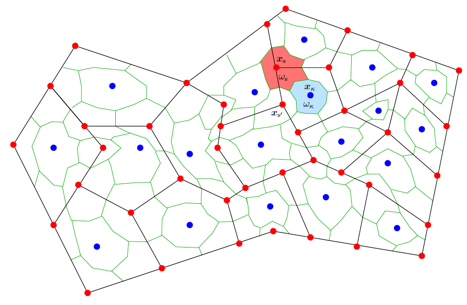
We aim now to reconstruct piecewise constant functions. To this end, we introduce a so-called mass lumping mesh $\mathcal{D}$ depending on additional parameters that appear to play an important role in practical applications [54]. Let $\kappa\in\mathcal{M}$, then introduce some weights $\left(\alpha_{\kappa,{\rm s}}\right)_{{\rm s}\in\mathcal{V}_{\kappa}}$ such that

(27) $$\alpha_{\kappa,{\rm s}}\geq 0,\quad\text{and}\quad\sum_{{\rm s}\in\mathcal{V}_{\kappa}}\alpha_{\kappa,{\rm s}}\leq 1,\quad\forall{\rm s}\in\mathcal{V}_{\kappa}.$$

Denoting by ${\rm meas}(\kappa)=\int_{\kappa}{\rm d}{\boldsymbol{x}}$ the volume of $\kappa$, then we define the quantities

(28) $$\begin{cases}m_{\kappa,{\rm s}}=\alpha_{\kappa,{\rm s}}{\rm meas}(\kappa),&\forall\kappa\in\mathcal{M},\forall{\rm s}\in\mathcal{V}_{\kappa},\\ m_{\rm s}=\sum_{\kappa\in\mathcal{M}_{\rm s}}m_{\kappa,{\rm s}},&\forall{\rm s}\in\mathcal{V},\\ m_{\kappa}={\rm meas}(\kappa)-\sum_{{\rm s}\in\mathcal{V}_{\kappa}}m_{\kappa,{\rm s}},&\forall\kappa\in\mathcal{M},\end{cases}$$

so that one has

$$\sum_{\beta\in\mathcal{M}\cup\mathcal{V}}m_{\beta}={\rm meas}(\Omega).$$

For all $\kappa\in\mathcal{M}$, we denote by $\omega_{\kappa}$ and $\omega_{\kappa,{\rm s}}$ some disjointed open subsets of $\kappa$, such that

$${\overline{\omega}}_{\kappa}\cup\left(\bigcup_{{\rm s}\in\mathcal{V}_{\kappa}}{\overline{\omega}}_{\kappa,{\rm s}}\right)={\overline{\kappa}},$$

and such that

$${\rm meas}(\omega_{\kappa})=m_{\kappa}\quad\text{and}\quad{\rm meas}(\omega_{\kappa,{\rm s}})=m_{\kappa,{\rm s}},\qquad\forall\kappa\in\mathcal{M},\;\forall{\rm s}\in\mathcal{V}_{\kappa}.$$

Note that such a decomposition always exists thanks to (27)–(28). Then we denote by

$$\omega_{\rm s}=\bigcup_{\kappa\in\mathcal{M}_{\rm s}}\omega_{\kappa,{\rm s}},\qquad\forall{\rm s}\in\mathcal{V}.$$

The mass-lumping mesh $\mathcal{D}$ is made of the cells $\omega_{\kappa}$ and $\omega_{\rm s}$ for $\kappa\in\mathcal{M}$ and ${\rm s}\in\mathcal{V}$. An illustration is presented in Figure 3.

Figure 3. The mass-lumping mesh $\mathcal{D}$ contains one cell $\omega_{\kappa}$ and $\omega_{\rm s}$ by degree of fredom. The mass repartition depends on the factors $\alpha_{\kappa,{\rm s}}$ introduced at (27).

In [54], a study focused on the repartition of the porous volume between nodes and centers is proposed, in the case of a coupled problem (transport of a species in the flow of a fluid in a porous medium). The influence of this repartition mainly concerns the transport part, and not the fluid flow. In the framework of the present paper, we numerically observe that this repartition has not a strong influence in the cases studied. However, since the function $\eta$ can vanish, the limit choice $m_{\kappa}=0$ (resp. $m_{\rm s}=0$) can lead to singular cases, and therefore must be prevented.

In what follows, we denote by

(29) $$\zeta_{\mathcal{D}}=\min_{\beta\in\mathcal{M}\cup\mathcal{V}}\frac{m_{\beta}}{\int_{\Omega}\pi_{\mathcal{T}}{\bf e}_{\beta}{\rm d}{\boldsymbol{x}}},$$

where ${\bf e}_{\beta}$, $\beta\in\mathcal{M}\cup\mathcal{V}$ is the unique element of $W_{\mathcal{D}}$ such that

$$\pi_{\mathcal{T}}{\bf e}_{\beta}({\boldsymbol{x}}_{\gamma})=\delta_{\beta}^{\gamma},\qquad\forall\gamma\in\mathcal{M}\cup\mathcal{V},$$

and $\delta_{\beta}^{\gamma}$ is the kronecker symbol.

We can now define the piecewise constant reconstruction operators $\pi_{\mathcal{D}}:W_{\mathcal{D}}\to L^{\infty}\cap{\rm BV}(\Omega)$ and $\pi_{\mathcal{M}}:W_{\mathcal{D}}\to L^{\infty}\cap{\rm BV}(\Omega)$ by

(30) $$\pi_{\mathcal{D}}({\boldsymbol{v}})({\boldsymbol{x}})=\sum_{\kappa\in\mathcal{M}}v_{\kappa}{\bf 1}_{\omega_{\kappa}}({\boldsymbol{x}})+\sum_{{\rm s}\in\mathcal{V}}v_{\rm s}{\bf 1}_{\omega_{\rm s}}({\boldsymbol{x}}),\qquad\forall{\boldsymbol{x}}\in\Omega,\quad\forall{\boldsymbol{v}}\in W_{\mathcal{D}},$$

and

(31) $$\pi_{\mathcal{M}}({\boldsymbol{v}})({\boldsymbol{x}})=\sum_{\kappa\in\mathcal{M}}v_{\kappa}{\bf 1}_{\kappa}({\boldsymbol{x}})\qquad\forall{\boldsymbol{x}}\in\Omega,\quad\forall{\boldsymbol{v}}\in W_{\mathcal{D}}.$$

Let $f:\mathbb{R}\to\mathbb{R}$ be a possibly nonlinear function, then denote by

$$f({\boldsymbol{v}})=\left(f(v_{\kappa}),f(v_{\rm s})\right)_{\kappa\in\mathcal{M},{\rm s}\in\mathcal{V}},\qquad\forall{\boldsymbol{v}}=\left(v_{\kappa},v_{\rm s}\right)_{\kappa\in\mathcal{M},{\rm s}\in\mathcal{V}}\in W_{\mathcal{D}}.$$

Notice that in general,

$$\pi_{\mathcal{T}}(f({\boldsymbol{v}}))\neq f(\pi_{\mathcal{T}}({\boldsymbol{v}}))\quad\text{and}\quad\boldsymbol{\nabla}_{\mathcal{T}}(f({\boldsymbol{v}}))\neq\boldsymbol{\nabla}f(\pi_{\mathcal{T}}({\boldsymbol{v}})),$$

but that

(32) $$\pi_{\mathcal{D}}(f({\boldsymbol{v}}))=f(\pi_{\mathcal{D}}({\boldsymbol{v}}))\quad\text{and }\quad\pi_{\mathcal{M}}(f({\boldsymbol{v}}))=f(\pi_{\mathcal{M}}({\boldsymbol{v}})),\qquad\forall{\boldsymbol{v}}\in W_{\mathcal{D}}.$$

2.1.2. Time-and-space discretizations and discrete functions

Let $N\geq 1$ and let $0=t_{0}<t_{1}<\dots<t_{N-1}<t_{N}={t_{\rm f}}$ be some subdivision of $[0,{t_{\rm f}}]$. We denote by ${\Delta t}_{n}=t_{n}-t_{n-1}$ for all $n\in\{1,\dots N\}$, by ${\boldsymbol{\Delta}t}=({\Delta t}_{1},\dots,{\Delta t}_{N})^{T}\in\mathbb{R}^{N},$ and by

(33) $${\overline{{\Delta t}}}=\max_{1\leq n\leq N}{\Delta t}_{n}.$$

The time and space discrete space is then defined by

$$W_{\mathcal{D},{\boldsymbol{\Delta}t}}=\left\{{\boldsymbol{v}}=\left(v_{\kappa}^{n},v_{\rm s}^{n}\right)_{\kappa\in\mathcal{M},{\rm s}\in\mathcal{V},1\leq n\leq N}\in\mathbb{R}^{N(\#\mathcal{M}+\#\mathcal{V})}\right\}.$$

For ${\boldsymbol{v}}\in W_{\mathcal{D},{\boldsymbol{\Delta}t}}$ and $n\in\{1,\dots,N\}$, we denote by

$${\boldsymbol{v}}^{n}=\left(v_{\kappa}^{n},v_{\rm s}^{n}\right)_{\kappa\in\mathcal{M},{\rm s}\in\mathcal{V}}\in W_{\mathcal{D}}.$$

We deduce from the space reconstruction operators $\pi_{\mathcal{D}}$, $\pi_{\mathcal{M}}$ and $\pi_{\mathcal{T}}$ some time and space reconstructions operators $\pi_{\mathcal{D},{\boldsymbol{\Delta}t}},\pi_{\mathcal{M},{\boldsymbol{\Delta}t}},\pi_{\mathcal{T},{\boldsymbol{\Delta}t}}:W_{\mathcal{D},{\boldsymbol{\Delta}t}}\to L^{\infty}(Q_{t_{\rm f}})$ mapping the elements of $W_{\mathcal{D},{\boldsymbol{\Delta}t}}$ into constant w.r.t. time functions defined by

$$\pi_{\mathcal{D},{\boldsymbol{\Delta}t}}{\boldsymbol{v}}(\cdot,t)=\pi_{\mathcal{D}}({\boldsymbol{v}}^{n}),\quad\pi_{\mathcal{M},{\boldsymbol{\Delta}t}}{\boldsymbol{v}}(\cdot,t)=\pi_{\mathcal{M}}({\boldsymbol{v}}^{n})\quad\text{and}\quad\pi_{\mathcal{T},{\boldsymbol{\Delta}t}}{\boldsymbol{v}}(\cdot,t)=\pi_{\mathcal{T}}({\boldsymbol{v}}^{n})$$

if $t\in(t_{n-1},t_{n}]$. The gradient reconstruction operator $\boldsymbol{\nabla}_{\mathcal{T},{\boldsymbol{\Delta}t}}:W_{\mathcal{D},{\boldsymbol{\Delta}t}}\to\left(L^{\infty}(Q_{t_{\rm f}})\right)^{d}$ is then defined by

$$\boldsymbol{\nabla}_{\mathcal{T},{\boldsymbol{\Delta}t}}{\boldsymbol{v}}=\boldsymbol{\nabla}\pi_{\mathcal{T},{\boldsymbol{\Delta}t}}{\boldsymbol{v}},\qquad\forall{\boldsymbol{v}}\in W_{\mathcal{D},{\boldsymbol{\Delta}t}}.$$

2.2. The nonlinear scheme for degenerate parabolic equations

For $\kappa\in\mathcal{M}$, we denote by ${\bf A}_{\kappa}=\left(a^{\kappa}_{{\rm s},{\rm s}^{\prime}}\right)_{{\rm s},{\rm s}^{\prime}\in\mathcal{V}_{\kappa}}\in\mathbb{R}^{\ell_{\kappa}\times\ell_{\kappa}}$ the symmetric positive definite matrix whose coefficients are defined by

(34) $$a_{{\rm s},{\rm s}^{\prime}}^{\kappa}=\int_{\kappa}{\boldsymbol{\Lambda}}({\boldsymbol{x}})\boldsymbol{\nabla}_{\mathcal{T}}{\bf e}_{\rm s}({\boldsymbol{x}})\cdot\boldsymbol{\nabla}_{\mathcal{T}}{\bf e}_{{\rm s}^{\prime}}({\boldsymbol{x}}){\rm d}{\boldsymbol{x}}=a^{\kappa}_{{\rm s}^{\prime},{\rm s}}.$$

It results from the relation

$$\pi_{\mathcal{T}}{\bf e}_{\kappa}({\boldsymbol{x}})+\sum_{{\rm s}\in\mathcal{V}_{\kappa}}\pi_{\mathcal{T}}{\bf e}_{\rm s}({\boldsymbol{x}})=1,\qquad\forall{\boldsymbol{x}}\in\kappa,\;\forall\kappa\in\mathcal{M},$$

that, for all ${\boldsymbol{u}},{\boldsymbol{v}}\in W_{\mathcal{D}}$ and all $\kappa\in\mathcal{M}$, one has

(35) $$\int_{\kappa}{\boldsymbol{\Lambda}}({\boldsymbol{x}})\boldsymbol{\nabla}_{\mathcal{T}}{\boldsymbol{u}}({\boldsymbol{x}})\cdot\boldsymbol{\nabla}_{\mathcal{T}}{\boldsymbol{v}}({\boldsymbol{x}}){\rm d}{\boldsymbol{x}}=\sum_{{\rm s}\in\mathcal{V}_{\kappa}}\sum_{{\rm s}^{\prime}\in\mathcal{V}_{\kappa}}a_{{\rm s},{\rm s}^{\prime}}^{\kappa}(u_{\kappa}-u_{\rm s})(v_{\kappa}-v_{{\rm s}^{\prime}}).$$

For $\kappa\in\mathcal{M}$, we denote by ${\boldsymbol{\delta}}_{\kappa}:W_{\mathcal{D}}\to\mathbb{R}^{\ell_{\kappa}}$ the linear operator defined by

$$\left({\boldsymbol{\delta}}_{\kappa}{\boldsymbol{v}}\right)_{\rm s}=v_{\kappa}-v_{\rm s},\qquad\forall{\rm s}\in\mathcal{V}_{\kappa},\;\forall{\boldsymbol{v}}\in W_{\mathcal{D}}.$$

With this notation, we obtain that (35) rewrites as

$$\int_{\kappa}{\boldsymbol{\Lambda}}({\boldsymbol{x}})\boldsymbol{\nabla}_{\mathcal{T}}{\boldsymbol{u}}({\boldsymbol{x}})\cdot\boldsymbol{\nabla}_{\mathcal{T}}{\boldsymbol{v}}({\boldsymbol{x}}){\rm d}{\boldsymbol{x}}={\boldsymbol{\delta}}_{\kappa}{\boldsymbol{v}}\cdot{\bf A}_{\kappa}{\boldsymbol{\delta}}_{\kappa}{\boldsymbol{u}},\qquad\forall{\boldsymbol{u}},{\boldsymbol{v}}\in W_{\mathcal{D}},\;\forall\kappa\in\mathcal{M}.$$

In order to deal with the nonlinearities of the problem, we introduce the sets $W^{\rm ad}_{\mathcal{D}}\subset W_{\mathcal{D}}$ and $W^{\rm ad}_{\mathcal{D},{\boldsymbol{\Delta}t}}\subset W_{\mathcal{D},{\boldsymbol{\Delta}t}}$ of the admissible states defined by

$${\boldsymbol{v}}\in W^{\rm ad}_{\mathcal{D}}\quad\text{iff}\qquad v_{\nu}\in{\mathcal{I}}_{p},\quad\forall\nu\in\mathcal{M}\cup\mathcal{V},$$

and

$${\boldsymbol{v}}\in W^{\rm ad}_{\mathcal{D},{\boldsymbol{\Delta}t}}\quad\text{iff}\qquad{\boldsymbol{v}}^{n}\in W^{\rm ad}_{\mathcal{D}},\quad\forall n\in\{1,\dots,N\},$$

while we denote by $W_{\mathcal{D}}^{\rm en}\subset W_{\mathcal{D}}$ the set of finite entropy vectors:

(36) $${\boldsymbol{v}}\in W^{\rm en}_{\mathcal{D}}\quad\text{iff}\quad\mathfrak{E}_{\mathcal{D}}({\boldsymbol{v}}):=\int_{\Omega}\left(\Gamma(\pi_{\mathcal{D}}{\boldsymbol{v}})+\pi_{\mathcal{D}}({\boldsymbol{v}})\pi_{\mathcal{D}}({\bf V})\right){\rm d}{\boldsymbol{x}}<\infty,$$

where ${\bf V}=(V_{\kappa},V_{\rm s})_{\kappa,{\rm s}}\in W_{\mathcal{D}}$ is defined by

(37) $$V_{\kappa}=V({\boldsymbol{x}}_{\kappa})\quad V_{\rm s}=V({\boldsymbol{x}}_{\rm s})\qquad\forall\kappa\in\mathcal{M},\forall{\rm s}\in\mathcal{V}.$$

It is easy to check that, thanks to assumptions $({\bf A}2)$ and to the definition (4) of the convex function $\Gamma$, one has $W^{\rm ad}_{\mathcal{D}}\subset W^{\rm en}_{\mathcal{D}}$.

Given ${\boldsymbol{u}}\in W_{\mathcal{D}}^{\rm ad}$ and ${\bf V}\in W_{\mathcal{D}}$, we define the discrete hydrostatic pressure ${\boldsymbol{h}}({\boldsymbol{u}})=\left(\mathfrak{h}_{\kappa}(u_{\kappa}),\mathfrak{h}_{\rm s}(u_{s})\right)_{\kappa,{\rm s}}\in W_{\mathcal{D}}$ by

(38) $$\mathfrak{h}_{\kappa}(u_{\kappa})=p(u_{\kappa})+V_{\kappa},\qquad\mathfrak{h}_{\rm s}(u_{\rm s})=p(u_{\rm s})+V_{\rm s},\qquad\forall\kappa\in\mathcal{M},\,\forall{\rm s}\in\mathcal{V}.$$

The initial data $u_{0}$ is discretized into an element ${\boldsymbol{u}}^{0}\in{W^{\rm en}_{\mathcal{D}}}$ by

(39) $$u_{\beta}^{0}=\frac{1}{m_{\beta}}\int_{\omega_{\beta}}u_{0}({\boldsymbol{x}}){\rm d}{\boldsymbol{x}},\qquad\forall\beta\in\mathcal{M}\cup\mathcal{V},$$

so that, thanks to (5),

(40) $$\int_{\Omega}\pi_{\mathcal{D}}({\boldsymbol{u}}^{0}){\rm d}{\boldsymbol{x}}=\int_{\Omega}u_{0}{\rm d}{\boldsymbol{x}}>0.$$

Let us state a first lemma that ensure that the discretized initial data has a finite discrete entropy.

Lemma 2.1.

Let $u_{0}\in L^{1}(\Omega)$ be such that $({\bf A}{4})$ holds, $V$ be such that $({\bf A}{5})$ holds, ${\boldsymbol{u}}^{0}$ be defined by (39), and ${\bf V}$ defined by (37). Then there exists $C$ depending only on $\|u_{0}\|_{L^{1}(\Omega)}$ and $\|\boldsymbol{\nabla}V\|_{L^{\infty}(\Omega)^{d}}$ such that

(41) $$\mathfrak{E}_{\mathcal{D}}({\boldsymbol{u}}^{0})\leq\mathfrak{E}(u_{0})+Ch_{\mathcal{T}}\leq\mathfrak{E}(u_{0})+C{\rm diam}(\Omega),$$

where the entropy functional $\mathfrak{E}$ is defined by (14) and its discrete counterpart $\mathfrak{E}_{\mathcal{D}}$ is defined by (36). In particular, ${\boldsymbol{u}}^{0}$ belongs to ${W^{\rm en}_{\mathcal{D}}}$.

Proof.

We deduce from Jensen inequality that

$$\Gamma(u^{0}_{\beta})\leq\frac{1}{m_{\beta}}\int_{\omega_{\beta}}\Gamma(u_{0}){\rm d}{\boldsymbol{x}},$$

whence, thanks to $({\bf A}{4})$ and to the definition (36) of the discrete entropy functional $\mathfrak{E}_{\mathcal{D}}$, one has

$$\mathfrak{E}_{\mathcal{D}}({\boldsymbol{u}}^{0})\leq\mathfrak{E}(u_{0})+\int_{\Omega}u_{0}(\pi_{\mathcal{D}}{\bf V}-V){\rm d}{\boldsymbol{x}}+\int_{\Omega}(\pi_{\mathcal{D}}{\boldsymbol{u}}^{0}-u_{0})\pi_{\mathcal{D}}{\bf V}{\rm d}{\boldsymbol{x}}.$$

The last term in the above inequality is equal to zero thanks to (40). The Lipschitz regularity of $V$ yields

$$\|\pi_{\mathcal{D}}{\bf V}-V\|_{L^{\infty}(\Omega)}\leq\|\boldsymbol{\nabla}V\|_{L^{\infty}(\Omega)^{d}}h_{\mathcal{T}},$$

so that

$$\mathfrak{E}_{\mathcal{D}}({\boldsymbol{u}}^{0})\leq\mathfrak{E}(u_{0})+\|u_{0}\|_{L^{1}(\Omega)}\|\boldsymbol{\nabla}V\|_{L^{\infty}(\Omega)^{d}}h_{\mathcal{T}}.$$

∎

With all this setting, we can present the scheme we will analyze in this contribution. For ${\boldsymbol{u}}\in W^{\rm ad}_{\mathcal{D},{\boldsymbol{\Delta}t}}$, we introduce the notation

(42) $$\eta_{\kappa,{\rm s}}^{n}=\frac{\eta(u^{n}_{\kappa})+\eta(u^{n}_{\rm s})}{2},\qquad\forall\kappa\in\mathcal{M},\;\forall{\rm s}\in\mathcal{V}_{\kappa},\forall n\in\{1,\dots,N\}.$$

Given ${\boldsymbol{u}}^{n-1}\in{W_{\mathcal{D}}^{\rm en}}$, the vector ${\boldsymbol{u}}^{n}\in W_{\mathcal{D}}^{\rm ad}$ is obtained by solving the following nonlinear system:

(43a) $$m_{\kappa}\frac{u_{\kappa}^{n}-u_{\kappa}^{n-1}}{{\Delta t}_{n}}+\sum_{{\rm s}\in\mathcal{V}_{\kappa}}F_{\kappa,{\rm s}}({\boldsymbol{u}}^{n})=0,\qquad\forall\kappa\in\mathcal{M},$$

(43b) $$m_{\rm s}\frac{u_{\rm s}^{n}-u_{\rm s}^{n-1}}{{\Delta t}_{n}}+\sum_{\kappa\in\mathcal{M}_{\rm s}}F_{{\rm s},\kappa}({\boldsymbol{u}}^{n})=0,\qquad\forall{\rm s}\in\mathcal{V},$$

(43c) $$F_{\kappa,{\rm s}}({\boldsymbol{u}}^{n})=\sqrt{\eta_{\kappa,{\rm s}}^{n}}\sum_{{\rm s}^{\prime}\in\mathcal{V}_{\kappa}}a^{\kappa}_{{\rm s},{\rm s}^{\prime}}\sqrt{\eta_{\kappa,{\rm s}^{\prime}}^{n}}\left(\mathfrak{h}_{\kappa}(u_{\kappa}^{n})-\mathfrak{h}_{{\rm s}^{\prime}}(u_{{\rm s}^{\prime}}^{n})\right),\quad\forall\kappa\in\mathcal{M},\;\forall{\rm s}\in\mathcal{V}_{\kappa},$$

(43d) $$F_{\kappa,{\rm s}}({\boldsymbol{u}}^{n})+F_{{\rm s},\kappa}({\boldsymbol{u}}^{n})=0,\qquad\forall\kappa\in\mathcal{M},\;\forall{\rm s}\in\mathcal{V}_{\kappa}.$$

The scheme (43) can be interpreted as a finite volume scheme, the conservation being established on the cells $\omega_{\kappa}$ and $\omega_{\rm s}$ for $\kappa\in\mathcal{M}$ and ${\rm s}\in\mathcal{V}$. As a direct consequence of the conservativity of the scheme, one has

(44) $$\int_{\Omega}\pi_{\mathcal{D}}({\boldsymbol{u}}^{n}){\rm d}{\boldsymbol{x}}=\int_{\Omega}\pi_{\mathcal{D}}({\boldsymbol{u}}^{n-1}){\rm d}{\boldsymbol{x}}.$$

However, contrarily to usual finite volume schemes, the fluxes $F_{\kappa,{\rm s}}^{n}$ are not issued from the computation of $\int_{\sigma}\eta(u)\Lambda\boldsymbol{\nabla}(p(u)+V)\cdot{\boldsymbol{n}}_{\sigma}$ on a specific boundary $\sigma$ between identified control volumes. They result from the variational formulation of the scheme and are viewed as fluxes between control volumes located at nodes and centers.

Defining, for all $\kappa\in\mathcal{M}$ and ${\boldsymbol{u}}=(u_{\kappa},u_{\rm s})_{\kappa,{\rm s}}\in W_{\mathcal{D}}$, the diagonal matrix ${\bf M}_{\kappa}({\boldsymbol{u}})\in\mathbb{R}^{\ell_{\kappa}\times\ell_{\kappa}}$ by

$$\left({\bf M}_{\kappa}({\boldsymbol{u}})\right)_{{\rm s},{\rm s}^{\prime}}=\begin{cases}\sqrt{\frac{\eta(u_{\kappa})+\eta(u_{\rm s})}{2}}&\text{ if }{\rm s}={\rm s}^{\prime},\\ 0&\text{ otherwise},\end{cases}$$

the systems (43) is equivalent to the following compact formulation: $\forall{\boldsymbol{v}}\in W_{\mathcal{D}}$,

(45) $$\int_{\Omega}\pi_{\mathcal{D}}{\boldsymbol{u}}^{n}\pi_{\mathcal{D}}{\boldsymbol{v}}{\rm d}{\boldsymbol{x}}+{\Delta t}_{n}\sum_{\kappa\in\mathcal{M}}{\boldsymbol{\delta}}_{\kappa}{\boldsymbol{h}}({\boldsymbol{u}}^{n})\cdot{\bf B}_{\kappa}({\boldsymbol{u}}^{n}){\boldsymbol{\delta}}_{\kappa}{\boldsymbol{v}}=\int_{\Omega}\pi_{\mathcal{D}}{\boldsymbol{u}}^{n-1}\pi_{\mathcal{D}}{\boldsymbol{v}}{\rm d}{\boldsymbol{x}},$$

where

(46) $${\bf B}_{\kappa}({\boldsymbol{u}}):={\bf M}_{\kappa}({\boldsymbol{u}}){\bf A}_{\kappa}{\bf M}_{\kappa}({\boldsymbol{u}}),\qquad\forall\kappa\in\mathcal{M},\;\forall{\boldsymbol{u}}\in W_{\mathcal{D}},$$

is a symmetric semi-positive matrix since ${\bf A}_{\kappa}$ and ${\bf M}_{\kappa}({\boldsymbol{u}})$ have this property.

2.3. Gradient flow interpretation for the scheme

The goal of this section is to transpose the formal variational structure pointed out in §1.2 to the discrete setting. A natural discretization of the manifold $\mathfrak{M}$ consists in

(47) $$\mathfrak{M}_{\mathcal{D}}=\left\{{\boldsymbol{u}}\in W_{\mathcal{D}}\;\left|\;\int_{\Omega}\pi_{\mathcal{D}}{\boldsymbol{u}}{\rm d}{\boldsymbol{x}}=\int_{\Omega}u_{0}{\rm d}{\boldsymbol{x}}\right\}\right.,$$

leading to

(48) $$T_{\boldsymbol{u}}\mathfrak{M}_{\mathcal{D}}=\left\{{\boldsymbol{v}}\in W_{\mathcal{D}}\;\left|\;\int_{\Omega}\pi_{\mathcal{D}}{\boldsymbol{v}}{\rm d}{\boldsymbol{x}}=0\right\}\right..$$

In order to define the discrete counterpart $\mathfrak{g}_{\mathcal{D},{\boldsymbol{u}}}$ of the metric tensor $\mathfrak{g}_{u}$ defined by (12)–(13), one needs a discrete counterpart of

• the classical $L^{2}(\Omega)$ scalar product: we will use

  $$({\boldsymbol{w}}_{1},{\boldsymbol{w}}_{2})\mapsto\int_{\Omega}\pi_{\mathcal{D}}{\boldsymbol{w}}_{1}\,\pi_{\mathcal{D}}{\boldsymbol{w}}_{2}{\rm d}{\boldsymbol{x}},\qquad\forall{\boldsymbol{w}}_{1},{\boldsymbol{w}}_{2}\in W_{\mathcal{D}};$$

• the weighted ${H}^{1}(\Omega)$ “scalar product” with weight $\eta(u)$: we use

  $$({\boldsymbol{w}}_{1},{\boldsymbol{w}}_{2})\mapsto\sum_{\kappa\in\mathcal{M}}{\boldsymbol{\delta}}_{\kappa}{\boldsymbol{w}}_{1}\cdot{\bf B}_{\kappa}({\boldsymbol{u}}){\boldsymbol{\delta}}_{\kappa}{\boldsymbol{w}}_{2},\qquad\forall{\boldsymbol{w}}_{1},{\boldsymbol{w}}_{2}\in W_{\mathcal{D}}.$$

This allows to define the discrete metric tensor $\mathfrak{g}_{\mathcal{D},{\boldsymbol{u}}}$ by: $\forall{\boldsymbol{u}}\in W_{\mathcal{D}}$, $\forall{\boldsymbol{w}}_{1},{\boldsymbol{w}}_{2}\in T_{\boldsymbol{u}}\mathfrak{M}_{\mathcal{D}}$,

(49) $$\mathfrak{g}_{\mathcal{D},{\boldsymbol{u}}}({\boldsymbol{w}}_{1},{\boldsymbol{w}}_{2})=\int_{\Omega}\pi_{\mathcal{D}}{\boldsymbol{w}}_{1}\pi_{\mathcal{D}}\boldsymbol{\phi}_{2}{\rm d}{\boldsymbol{x}}=\int_{\Omega}\pi_{\mathcal{D}}\boldsymbol{\phi}_{1}\pi_{\mathcal{D}}{\boldsymbol{v}}_{2}{\rm d}{\boldsymbol{x}}=\sum_{\kappa\in\mathcal{M}}{\boldsymbol{\delta}}_{\kappa}\boldsymbol{\phi}_{1}\cdot{\bf B}_{\kappa}({\boldsymbol{u}}){\boldsymbol{\delta}}_{\kappa}\boldsymbol{\phi}_{2},$$

where $\boldsymbol{\phi}_{i}\in W_{\mathcal{D}}$ solves the discrete counterpart of (13), that is

(50) $$\sum_{\kappa\in\mathcal{M}}{\boldsymbol{\delta}}_{\kappa}\boldsymbol{\phi}_{i}\cdot{\bf B}_{\kappa}({\boldsymbol{u}}){\boldsymbol{\delta}}_{\kappa}\boldsymbol{\psi}=\int_{\Omega}\pi_{\mathcal{D}}{\boldsymbol{w}}_{i}\,\pi_{\mathcal{D}}\boldsymbol{\psi}\,{\rm d}{\boldsymbol{x}},\qquad\forall\boldsymbol{\psi}\in W_{\mathcal{D}}.$$

In this setting, we can define the semi-discrete in space gradient flow by

(51) $$\mathfrak{g}_{\mathcal{D},{\boldsymbol{u}}}(\partial_{t}{\boldsymbol{u}},{\boldsymbol{w}})=\int_{\Omega}\pi_{\mathcal{D}}(\partial_{t}{\boldsymbol{u}})\,\pi_{\mathcal{D}}{\boldsymbol{v}}\,{\rm d}{\boldsymbol{x}}\\ =\mathfrak{g}_{\mathcal{D},{\boldsymbol{u}}}(-\boldsymbol{\nabla}_{u}\mathfrak{E}({\boldsymbol{u}}),{\boldsymbol{w}})=\int_{\Omega}\pi_{\mathcal{D}}{\boldsymbol{h}}({\boldsymbol{u}})\,\pi_{\mathcal{D}}{\boldsymbol{w}}\,{\rm d}{\boldsymbol{x}}=\sum_{\kappa}{\boldsymbol{\delta}}_{\kappa}{\boldsymbol{h}}({\boldsymbol{u}})\cdot{\bf B}_{\kappa}({\boldsymbol{u}}){\boldsymbol{\delta}}_{\kappa}{\boldsymbol{v}},$$

where ${\boldsymbol{v}}$ solve the discrete elliptic problem

$$\sum_{\kappa\in\mathfrak{M}}{\boldsymbol{\delta}}_{\kappa}{\boldsymbol{v}}\cdot{\bf B}_{\kappa}({\boldsymbol{u}}){\boldsymbol{\delta}}_{\kappa}\boldsymbol{\psi}=\int_{\Omega}\pi_{\mathcal{D}}{\boldsymbol{w}}\,\pi_{\mathcal{D}}\boldsymbol{\psi}\,{\rm d}{\boldsymbol{x}},\qquad\forall\boldsymbol{\psi}\in W_{\mathcal{D}}.$$

In order to recover (45) from (51), one applies the backward Euler scheme.

Remark 2.2.

In their seminal paper [65], Jordan, Kinderlehrer and Otto proposed to approximate the solution of gradient flows thanks to the minimizing movement scheme

(52) $${\boldsymbol{u}}^{n}\in\underset{{\boldsymbol{u}}\in\mathfrak{M}_{\mathcal{D}}}{\rm argmin}\Big{\{}\frac{\mathfrak{d}({\boldsymbol{u}},{\boldsymbol{u}}^{n-1})}{2{\Delta t}}+\mathfrak{E}_{\mathcal{D}}({\boldsymbol{u}})\Big{\}},$$

where $\mathfrak{d}$ denotes the distance on $\mathfrak{M}_{\mathcal{D}}$ induced by the metric tensor field $\mathfrak{g}_{\mathcal{D}}$. Several practical and theoretical difficulties arise when one aims at using (52). First of all, the Riemannian structure is formal, even in the continuous case. It is unclear if one can define rigorously a distance $\mathfrak{d}$ if $\eta(0)=0$ even if $\eta$ is concave (cf. [43, 81]). But even if $\mathfrak{d}$ is a distance, yielding a metric structure for $\mathfrak{M}_{\mathcal{D}}$, computing this distance is a complex problem we avoid by using an backward Euler scheme rather than (52).

2.4. Main results

The first result we want to point out concerns the scheme for a fixed mesh. The following theorem states that the scheme (43) admits at least one solution, and justifies the free energy diminishing denomination for the scheme.

Theorem 2.3.

Let ${\boldsymbol{u}}^{n-1}\in W_{\mathcal{D}}^{\rm en}$, then there exists (at least) one vector ${\boldsymbol{u}}^{n}\in W_{\mathcal{D}}^{\rm ad}$ solution to the system (43), and the following dissipation property holds:

(53) $$\mathfrak{E}_{\mathcal{D}}({\boldsymbol{u}}^{n})+{\Delta t}_{n}\sum_{\kappa\in\mathcal{M}}{\boldsymbol{\delta}}_{\kappa}{\boldsymbol{h}}({\boldsymbol{u}}^{n})\cdot{\bf B}_{\kappa}({\boldsymbol{u}}^{n}){\boldsymbol{\delta}}_{\kappa}{\boldsymbol{h}}({\boldsymbol{u}}^{n})\leq\mathfrak{E}_{\mathcal{D}}({\boldsymbol{u}}^{n-1}),$$

where $\mathfrak{E}_{\mathcal{D}}$ is defined by (36) and ${\boldsymbol{h}}({\boldsymbol{u}}^{n})=\left(\mathfrak{h}_{\kappa}(u_{\kappa}^{n}),\mathfrak{h}_{\rm s}(u_{\rm s}^{n})\right)_{\kappa,{\rm s}}$ is defined by (38).

Since ${\boldsymbol{u}}^{0}\in W_{\mathcal{D}}^{\rm en}$ and since $W_{\mathcal{D}}^{\rm ad}\subset W_{\mathcal{D}}^{\rm en}$, Theorem 2.3 allows to define the iterated solution ${\boldsymbol{u}}=({\boldsymbol{u}}^{n})_{1\leq n\leq N}\in W_{\mathcal{D},{\boldsymbol{\Delta}t}}^{\rm ad}$ to the scheme (43).

The proof of Theorem 2.3 is contained in §3, together with some supplementary material that allows to carry out the convergence analysis when the discretization steps tend to $0$. More precisely, we consider a sequence $\left(\mathcal{D}_{m}\right)_{m\geq 1}=\left(\mathcal{M}_{m},\mathcal{T}_{m}\right)_{m\geq 1}$ of discretizations of $\Omega$ as introduced in §2.1.1, such that

(54a) $$h_{\mathcal{T}_{m}}=\max_{T\in\mathcal{T}_{m}}h_{T}\underset{m\to+\infty}{\longrightarrow}0,$$

and such that there exists $$\theta^{\star}>0 \ell^{\star}>0$$ and satisfying

(54b) $$\sup_{m\geq 1}\theta_{\mathcal{T}_{m}}\leq\theta^{\star},\qquad\sup_{m\geq 1}\ell_{\mathcal{D}_{m}}\leq\ell^{\star},$$

where $$\theta_{\mathcal{T}_{m}} \ell_{\mathcal{D}_{m}}$$ and are defined by (21) and (24) respectively.

Even though it can be avoided in some specific situations, we also do the following assumption, allowing to circumvent some technical difficulties:

(54c) $$\inf_{m\geq 1}\zeta_{\mathcal{D}_{m}}=\zeta^{\star}>0.$$

This means that there is a minimum ratio of volume allocated to the cell centers and to the nodes in the mass lumping procedure.

Concerning the time-discretizations, we consider a sequence $\left({\boldsymbol{\Delta}t}_{m}\right)_{m\geq 1}$ of discretizations of $(0,{t_{\rm f}})$ as prescribed in §2.1.2 :

$${\boldsymbol{\Delta}t}_{m}=\left({\Delta t}_{1,m},\dots,{\Delta t}_{N_{m},m}\right),\qquad\forall m\geq 1.$$

We assume that the time discretization step tends to $0$, i.e.,

(54d) $${\overline{{\Delta t}}}_{m}=\max_{1\leq n\leq N_{m}}{\Delta t}_{n,m}\underset{m\to+\infty}{\longrightarrow}0.$$

Theorem 2.4.

Let $\left(\mathcal{D}_{m},{\boldsymbol{\Delta}t}_{m}\right)_{m}$ be a sequence of discretizations of $Q_{t_{\rm f}}$ satisfying Assumptions (54), and let $\left({\boldsymbol{u}}_{m}\right)_{m\geq 1}$, with ${\boldsymbol{u}}_{m}\in W_{\mathcal{D}_{m},{\boldsymbol{\Delta}t}_{m}}^{\rm ad}$, be a corresponding sequence of iterated discrete solutions, then

$$\pi_{\mathcal{D}_{m},{\boldsymbol{\Delta}t}_{m}}{\boldsymbol{u}}_{m}\underset{m\to+\infty}{\longrightarrow}u\quad\text{strongly in }L^{1}(Q_{t_{\rm f}}),$$

where $u$ is the unique weak solution to (1) in the sense of Definition 1.

Proving the Theorem 2.4 is the purpose of §4. The practical implementation of the scheme (43) is discussed in §5, where we also give evidences of the efficiency of the scheme.

3. Proof of Theorem 2.3 and additional estimates

In order to ease the reading of the paper, several technical lemmas have been postponed to Appendix.

3.1. One-step A priori estimates

Lemma 3.1.

Let ${\boldsymbol{u}}^{n-1}\in W_{\mathcal{D}}^{\rm en}$, and let ${\boldsymbol{u}}^{n}\in W_{\mathcal{D}}^{\rm ad}$ be a solution to the scheme (43), then (53) holds.

Proof.

Substituting ${\boldsymbol{v}}$ by ${\boldsymbol{h}}({\boldsymbol{u}}^{n})=\left(\mathfrak{h}_{\kappa}(u_{\kappa}^{n}),\mathfrak{h}_{\rm s}(u_{\rm s}^{n})\right)_{\kappa,{\rm s}}$ defined by (38) in (45) yields

(55) $$\int_{\Omega}\!\!\left(\pi_{\mathcal{D}}{\boldsymbol{u}}^{n}-\pi_{\mathcal{D}}{\boldsymbol{u}}^{n-1}\right)\pi_{\mathcal{D}}{\boldsymbol{h}}({\boldsymbol{u}}^{n}){\rm d}{\boldsymbol{x}}+{\Delta t}_{n}\!\!\sum_{\kappa\in\mathcal{M}}{\boldsymbol{\delta}}_{\kappa}{\boldsymbol{h}}({\boldsymbol{u}}^{n})\cdot{\bf B}_{\kappa}({\boldsymbol{u}}^{n}){\boldsymbol{\delta}}_{\kappa}{\boldsymbol{h}}({\boldsymbol{u}}^{n})=0.$$

It follows from the convexity of $\Gamma$ that

$$\Gamma(a)-\Gamma(b)\leq(a-b)\left(p(a)-p(1)\right),\qquad\forall\;a,b\in\mathbb{R}\;\text{ s.t. }\;\Gamma(a),\Gamma(b)<+\infty.$$

Hence, using (44), one has

$$\int_{\Omega}\left(\pi_{\mathcal{D}}{\boldsymbol{u}}^{n}-\pi_{\mathcal{D}}{\boldsymbol{u}}^{n-1}\right)\pi_{\mathcal{D}}{\boldsymbol{h}}({\boldsymbol{u}}^{n}){\rm d}{\boldsymbol{x}}\\ =\int_{\Omega}\left(\pi_{\mathcal{D}}{\boldsymbol{u}}^{n}-\pi_{\mathcal{D}}{\boldsymbol{u}}^{n-1}\right)\left(p(\pi_{\mathcal{D}}{\boldsymbol{u}}^{n})+\pi_{\mathcal{D}}({\bf V})\right){\rm d}{\boldsymbol{x}}\\ \geq\int_{\Omega}\left(\Gamma(\pi_{\mathcal{D}}{\boldsymbol{u}}^{n})-\Gamma(\pi_{\mathcal{D}}{\boldsymbol{u}}^{n-1})+\pi_{\mathcal{D}}({\boldsymbol{u}}^{n}-{\boldsymbol{u}}^{n-1})\pi_{\mathcal{D}}{\bf V}\right){\rm d}{\boldsymbol{x}}\\ =\mathfrak{E}_{\mathcal{D}}({\boldsymbol{u}}^{n})-\mathfrak{E}_{\mathcal{D}}({\boldsymbol{u}}^{n-1}).$$

Using this inequality in (55) provides (53). ∎

Lemma 3.2.

For all $\epsilon>0$, there exists $C_{\epsilon}\in\mathbb{R}$ depending on $\epsilon$ and $p$ such that

$$|u|\leq\epsilon\Gamma(u)+C_{\epsilon},\qquad\forall u\in W_{\mathcal{D}}^{\rm en}.$$

Proof.

Fix $\epsilon>0$, then in view of Assumption (A2), the intermediate value theorem ensures the existence of $u_{\epsilon}\geq 1$ such that $p(u_{\epsilon})=p(1)+1/\epsilon$. Then for all $u\in{\overline{{\mathcal{I}}}}_{p}$, one has

$$\Gamma(u)=\int_{1}^{u}(p(a)-p(1)){\rm d}a=\Gamma(u_{\epsilon})+\int_{u_{\epsilon}}^{u}(p(a)-p(1)){\rm d}a.$$

The function $p$ being increasing, we deduce that

$$\Gamma(u)\geq\Gamma(u_{\epsilon})+(p(u_{\epsilon})-p(1))|u-u_{\epsilon}|\geq\Gamma(u_{\epsilon})+\frac{1}{\epsilon}\left(|u|-|u_{\epsilon}|\right),\qquad\forall u\in{\overline{{\mathcal{I}}}}_{p}.$$

Lemma 3.2 follows with $C_{\epsilon}=|u_{\epsilon}|-\epsilon\Gamma(u_{\epsilon}).$ ∎

Lemma 3.3.

For all $\epsilon>0$, there exists $C_{\epsilon}\in\mathbb{R}$ depending on $\epsilon$, $\eta$ and $\Gamma$ such that

$$\eta(u)\leq\epsilon\Gamma(u)+C_{\epsilon},\qquad\forall u\in{\overline{{\mathcal{I}}}}_{p}.$$

Proof.

The function $u\mapsto\frac{\eta(u)}{\Gamma(u)}$ tends to $0$ as $|u|\to\infty$ thanks to Assumption (A6). Let $\epsilon>0$, then there exists $r_{\epsilon}>0$ such that

$$|u|>r_{\epsilon}\quad\implies\quad 0\leq\eta(u)\leq\epsilon\Gamma(u).$$

The function $\eta$ being continuous and nonnegative according to Assumption (A1), we know that

$$0\leq C_{\epsilon}:=\max_{u\in[-r_{\epsilon},r_{\epsilon}]}\eta(u)<+\infty.$$

The result of Lemma 3.3 follows. ∎

Lemma 3.4.

There exist $C_{1}$ and $C_{2}$ depending only on $p$, $V$ and $\Omega$ such that

(56) $$\frac{1}{2}\mathfrak{E}_{\mathcal{D}}({\boldsymbol{u}})+C_{1}\leq\int_{\Omega}\Gamma(\pi_{\mathcal{D}}{\boldsymbol{u}}){\rm d}{\boldsymbol{x}}\leq 2\mathfrak{E}_{\mathcal{D}}({\boldsymbol{u}})+C_{2},\qquad\forall{\boldsymbol{u}}\in W_{\mathcal{D}}^{\rm en}.$$

In particular, the discrete entropy functional $\mathfrak{E}_{\mathcal{D}}$ is bounded from below uniformly w.r.t. the discretization $\mathcal{D}$.

Proof.

Recall that the discrete entropy functional $\mathfrak{E}_{\mathcal{D}}$ is defined by

$$\mathfrak{E}_{\mathcal{D}}({\boldsymbol{u}})=\int_{\Omega}\left(\Gamma(\pi_{\mathcal{D}}{\boldsymbol{u}})+\pi_{\mathcal{D}}{\bf V}\,\pi_{\mathcal{D}}{\boldsymbol{u}}\right){\rm d}{\boldsymbol{x}},\qquad\forall{\boldsymbol{u}}\in W_{\mathcal{D}}^{\rm en}.$$

Hence, one has

(57) $$\int_{\Omega}\Gamma(\pi_{\mathcal{D}}{\boldsymbol{u}}){\rm d}{\boldsymbol{x}}\leq\mathfrak{E}_{\mathcal{D}}({\boldsymbol{u}})+\|\pi_{\mathcal{D}}{\bf V}\|_{L^{\infty}(\Omega)}\|\pi_{\mathcal{D}}{\boldsymbol{u}}\|_{L^{1}(\Omega)},\qquad\forall{\boldsymbol{u}}\in W_{\mathcal{D}}^{\rm en}.$$

Let $\epsilon>0$ a parameter to be fixed later on. Thanks to Lemma 3.2, there exists a quantity $C_{\epsilon}$ depending only on $p$ and $\epsilon$ such that

$$|u|\leq\epsilon\Gamma(u)+C_{\epsilon},\qquad\forall u\in{\overline{{\mathcal{I}}}}_{p},$$

ensuring that

(58) $$\|\pi_{\mathcal{D}}{\boldsymbol{u}}\|_{L^{1}(\Omega)}\leq\epsilon\int_{\Omega}\Gamma(\pi_{\mathcal{D}}{\boldsymbol{u}}){\rm d}{\boldsymbol{x}}+C_{\epsilon}{\rm meas}(\Omega),\qquad\forall{\boldsymbol{u}}\in W_{\mathcal{D}}^{\rm en}.$$

On the other hand, Assumption (A5) together with the definition (37) of ${\bf V}=\left(V_{\kappa},V_{\rm s}\right)_{\kappa,{\rm s}}$ ensure that

$$\|\pi_{\mathcal{D}}{\bf V}\|_{L^{\infty}(\Omega)}\leq\|V\|_{\infty}.$$

Setting $\epsilon=\frac{1}{2\|V\|_{\infty}}$ in (58) and injecting the resulting estimate in (57) ends the proof of the second inequality of (56). The proof of the first inequality of (56) being similar, it is left to the reader. ∎

Lemma 3.5.

There exists $C$ depending only on ${\boldsymbol{\Lambda}}$, $\Omega$, $\theta_{\mathcal{T}}$, $\zeta_{\mathcal{D}}$, $\ell_{\mathcal{D}}$, $\eta$, $p$ and $V$ such that, for all ${\boldsymbol{v}}=(v_{\kappa},v_{\rm s})_{\kappa,{\rm s}}\in W_{\mathcal{D}}^{\rm ad}$, one has

(59) $$\sum_{\kappa\in\mathcal{M}}\sum_{{\rm s}\in\mathcal{V}_{\kappa}}\left(\sum_{{\rm s}^{\prime}\in\mathcal{V}_{\kappa}}|a^{\kappa}_{{\rm s},{\rm s}^{\prime}}|\right)\eta_{\kappa,{\rm s}}({\boldsymbol{v}})\left(p(v_{\kappa})-p(v_{\rm s})\right)^{2}\\ \leq C\left(1+\mathfrak{E}_{\mathcal{D}}({\boldsymbol{v}})+\sum_{\kappa\in\mathcal{M}}{\boldsymbol{\delta}}_{\kappa}{\boldsymbol{h}}({\boldsymbol{v}})\cdot{\bf B}_{\kappa}({\boldsymbol{v}}){\boldsymbol{\delta}}_{\kappa}{\boldsymbol{h}}({\boldsymbol{v}})\right),$$

where we have set $\eta_{\kappa,{\rm s}}({\boldsymbol{v}})=\frac{\eta(v_{\kappa})+\eta(v_{\rm s})}{2}$ for all $\kappa\in\mathcal{M}$ and all ${\rm s}\in\mathcal{V}_{\kappa}$.

Proof.

Let ${\boldsymbol{v}}\in W_{\mathcal{D}}^{\rm ad}\subset W_{\mathcal{D}}^{\rm en}$, then it follows from the definition (38) of ${\boldsymbol{h}}({\boldsymbol{v}})=\left(\mathfrak{h}_{\kappa}(v_{\kappa}),\mathfrak{h}_{\rm s}(v_{s})\right)_{\kappa,{\rm s}}\in W_{\mathcal{D}}$ that

$${\boldsymbol{\delta}}_{\kappa}p({\boldsymbol{v}})\cdot{\bf B}_{\kappa}({\boldsymbol{v}}){\boldsymbol{\delta}}_{\kappa}p({\boldsymbol{v}})\leq 2{\boldsymbol{\delta}}_{\kappa}{\boldsymbol{h}}({\boldsymbol{v}})\cdot{\bf B}_{\kappa}({\boldsymbol{v}}){\boldsymbol{\delta}}_{\kappa}{\boldsymbol{h}}({\boldsymbol{v}})+2{\boldsymbol{\delta}}_{\kappa}{\bf V}\cdot{\bf B}_{\kappa}({\boldsymbol{v}}){\boldsymbol{\delta}}_{\kappa}{\bf V},\qquad\forall\kappa\in\mathcal{M}.$$

It follows from Lemma A.2 that there exists $C$ depending only on ${\boldsymbol{\Lambda}}$, $\theta_{\mathcal{T}}$ and $\ell_{\mathcal{D}}$ such that

$$\sum_{{\rm s}\in\mathcal{V}_{\kappa}}\left(\sum_{{\rm s}^{\prime}\in\mathcal{V}_{\kappa}}|a^{\kappa}_{{\rm s},{\rm s}^{\prime}}|\right)\eta_{\kappa,{\rm s}}({\boldsymbol{v}})\left(p(v_{\kappa})-p(v_{\rm s})\right)^{2}\leq C{\boldsymbol{\delta}}_{\kappa}p({\boldsymbol{v}})\cdot{\bf B}_{\kappa}({\boldsymbol{v}}){\boldsymbol{\delta}}_{\kappa}p({\boldsymbol{v}}),\qquad\forall\kappa\in\mathcal{M}.$$

Therefore, it only remains to prove that

(60) $$\sum_{\kappa\in\mathcal{M}}{\boldsymbol{\delta}}_{\kappa}{\bf V}\cdot{\bf B}_{\kappa}({\boldsymbol{v}}){\boldsymbol{\delta}}_{\kappa}{\bf V}\leq\mathfrak{E}_{\mathcal{D}}({\boldsymbol{v}})+C,$$

for some $C$ depending only on the prescribed data. Using Lemma A.3, we get that

(61) $$\sum_{\kappa\in\mathcal{M}}{\boldsymbol{\delta}}_{\kappa}{\bf V}\cdot{\bf B}_{\kappa}({\boldsymbol{v}}){\boldsymbol{\delta}}_{\kappa}{\bf V}\leq\sum_{\kappa\in\mathcal{M}}\max_{{\rm s}\in\mathcal{V}_{\kappa}}\eta_{\kappa,{\rm s}}({\boldsymbol{v}})\sum_{{\rm s}\in\mathcal{V}_{\kappa}}\left(\sum_{{\rm s}^{\prime}\in\mathcal{V}_{\kappa}}|a_{{\rm s},{\rm s}^{\prime}}^{\kappa}|\right)\left(V_{\kappa}-V_{\rm s}\right)^{2}.$$

It results from Lemma A.2 that for all $\kappa\in\mathcal{M}$,

(62) $$\sum_{{\rm s}\in\mathcal{V}_{\kappa}}\left(\sum_{{\rm s}^{\prime}\in\mathcal{V}_{\kappa}}|a_{{\rm s},{\rm s}^{\prime}}^{\kappa}|\right)\left(V_{\kappa}-V_{\rm s}\right)^{2}\leq C\int_{\kappa}\boldsymbol{\nabla}_{\mathcal{T}}{\bf V}\cdot{\boldsymbol{\Lambda}}\boldsymbol{\nabla}_{\mathcal{T}}{\bf V}{\rm d}{\boldsymbol{x}}\leq C|\kappa|\lambda^{\star}\|\boldsymbol{\nabla}V\|_{\infty}^{2}.$$

Denote by ${\overline{\eta}}({\boldsymbol{v}})=\left({\overline{\eta}}_{\kappa}({\boldsymbol{v}}),{\overline{\eta}}_{\rm s}({\boldsymbol{v}})\right)_{\kappa,{\rm s}}\in W_{\mathcal{D}}$ the vector defined by

$${\overline{\eta}}_{\kappa}({\boldsymbol{v}})=\max\left(\eta(v_{k});\max_{{\rm s}^{\prime}\in\mathcal{V}_{\kappa}}\eta(v_{\rm s}^{\prime})\right),\qquad{\overline{\eta}}_{\rm s}({\boldsymbol{v}})=0,\qquad\forall\kappa\in\mathcal{M},\;\forall{\rm s}\in\mathcal{V},$$

and remark that

$$\max_{{\rm s}\in\mathcal{V}_{\kappa}}\eta_{\kappa,{\rm s}}({\boldsymbol{v}})\leq{\overline{\eta}}_{\kappa}({\boldsymbol{v}}),\qquad\forall\kappa\in\mathcal{M}.$$

Hence, we deduce using (62) in (61) that

$$\sum_{\kappa\in\mathcal{M}}{\boldsymbol{\delta}}_{\kappa}{\bf V}\cdot{\bf B}_{\kappa}({\boldsymbol{v}}){\boldsymbol{\delta}}_{\kappa}{\bf V}\leq C\int_{\Omega}\pi_{\mathcal{M}}{\overline{\eta}}({\boldsymbol{v}}){\rm d}{\boldsymbol{x}},$$

for some $C$ depending only on $\theta_{\mathcal{T}}$, ${\boldsymbol{\Lambda}}$, $\ell_{\mathcal{D}}$ and $\|\boldsymbol{\nabla}V\|_{\infty}$, the operator $\pi_{\mathcal{M}}$ being defined by (31). Let us now use Lemma A.8 to obtain that

(63) $$\sum_{\kappa\in\mathcal{M}}{\boldsymbol{\delta}}_{\kappa}{\bf V}\cdot{\bf B}_{\kappa}({\boldsymbol{v}}){\boldsymbol{\delta}}_{\kappa}{\bf V}\leq{\widetilde{C}}\int_{\Omega}\pi_{\mathcal{D}}\eta({\boldsymbol{v}}){\rm d}{\boldsymbol{x}}$$

for some ${\widetilde{C}}$ depending only on the prescribed data, namely $\theta_{\mathcal{T}}$, ${\boldsymbol{\Lambda}}$, $\ell_{\mathcal{D}}$, $\zeta_{\mathcal{D}}$ and $\|\boldsymbol{\nabla}V\|_{\infty}$. Using Lemma 3.3, we know that for all $\epsilon>0$, there exists $C_{\epsilon}$ depending only on $\epsilon$, $\eta$, $\Gamma$ and ${\rm meas}(\Omega)$ such that

$$\int_{\Omega}\pi_{\mathcal{D}}\eta({\boldsymbol{v}}){\rm d}{\boldsymbol{x}}\leq\epsilon\int_{\Omega}\Gamma(\pi_{\mathcal{D}}{\boldsymbol{v}}){\rm d}{\boldsymbol{x}}+C_{\epsilon}.$$

Combining this result with Lemma 3.4 and (63), we deduce that for all $\epsilon>0$, there exists $C_{\epsilon}$ depending only on $\epsilon$, ${\boldsymbol{\Lambda}}$, $\Omega$, $\theta_{\mathcal{T}}$, $\zeta_{\mathcal{D}}$, $\ell_{\mathcal{D}}$, $\eta$, $p$ and $V$ such that

$$\sum_{\kappa\in\mathcal{M}}{\boldsymbol{\delta}}_{\kappa}{\bf V}\cdot{\bf B}_{\kappa}({\boldsymbol{v}}){\boldsymbol{\delta}}_{\kappa}{\bf V}\leq\epsilon{\widetilde{C}}\mathfrak{E}_{\mathcal{D}}({\boldsymbol{v}})+C_{\epsilon},\qquad\forall{\boldsymbol{v}}\in W_{\mathcal{D}}^{\rm en}.$$

We obtain (60) by choosing $\epsilon=\frac{1}{{\widetilde{C}}}$. This ends the proof of Lemma 3.5. ∎

Lemma 3.6.

Let ${\boldsymbol{u}}^{n-1}\in W_{\mathcal{D}}^{\rm en}$, and let ${\boldsymbol{u}}^{n}\in W_{\mathcal{D}}^{\rm ad}$ be a solution to the scheme (43). There exist $C_{1}$ and $C_{2}$ depending on ${\Delta t}_{n}$, ${\boldsymbol{\Lambda}}$, $\Omega$, $\theta_{\mathcal{T}}$, $\zeta_{\mathcal{D}}$, $\ell_{\mathcal{D}}$, $\eta$, $p$ and $V$ such that

$$\sum_{\kappa\in\mathcal{M}}\sum_{{\rm s}\in\mathcal{V}_{\kappa}}\left(\sum_{{\rm s}^{\prime}\in\mathcal{V}_{\kappa}}|a^{\kappa}_{{\rm s},{\rm s}^{\prime}}|\right)\eta_{\kappa,{\rm s}}^{n}\left(p(u_{\kappa}^{n})-p(u_{\rm s}^{n})\right)^{2}\\ \leq C_{1}\left(1+\mathfrak{E}_{\mathcal{D}}({\boldsymbol{u}}^{n-1})\right)\leq C_{2}\left(1+\int_{\Omega}\Gamma(\pi_{\mathcal{D}}{\boldsymbol{u}}^{n-1}){\rm d}{\boldsymbol{x}}\right).$$

Proof.

Since ${\boldsymbol{u}}^{n}$ is a solution of the scheme (43), the nonlinear discrete stability estimate (53) holds. Therefore, taking (53) into account in (59) yields

$$\sum_{\kappa\in\mathcal{M}}\sum_{{\rm s}\in\mathcal{V}_{\kappa}}\left(\sum_{{\rm s}^{\prime}\in\mathcal{V}_{\kappa}}|a^{\kappa}_{{\rm s},{\rm s}^{\prime}}|\right)\eta_{\kappa,{\rm s}}^{n}\left(p(u_{\kappa}^{n})-p(u_{\rm s}^{n})\right)^{2}\leq C_{1}\left(1+\mathfrak{E}_{\mathcal{D}}({\boldsymbol{u}}^{n-1})\right)$$

for some $C_{1}$ depending on the prescribed data. Then it only remains to use Lemma 3.4 to conclude the proof of Lemma 3.6. ∎

3.2. Existence of a discrete solution

The scheme (43) can be rewritten in the form of a nonlinear system

$$\mathcal{F}({\boldsymbol{u}}^{n})={\bf 0}_{\mathbb{R}^{\#\mathcal{M}+\#\mathcal{V}}}.$$

In the case where $p(0)=-\infty$, the function $\mathcal{F}$ is continuous on $W_{\mathcal{D}}^{\rm ad}$, but not uniformly continuous. The existence proof for a discrete solution we propose relies on a topological degree argument (see e.g. [73, 41]), whence we need to restrict the set of the possible ${\boldsymbol{u}}^{n}$ for recovering the uniform continuity by avoiding the singularity near $0$. This is the purpose of the following lemma, which is an adaptation of [34, Lemma 3.10].

Lemma 3.7.

Let ${\boldsymbol{u}}^{n-1}\in W_{\mathcal{D}}^{\rm en}$ be such that $\int_{\Omega}\pi_{\mathcal{D}}{\boldsymbol{u}}^{n-1}{\rm d}{\boldsymbol{x}}>0$ and let ${\boldsymbol{u}}^{n}$ be a solution to the scheme (43). Assume that $p(0)=-\infty$, then there exists $\epsilon_{\mathcal{D},{\Delta t}_{n}}>0$ depending on ${\Delta t}_{n}$, $\mathcal{D}$, ${\boldsymbol{\Lambda}}$, $\Omega$, $\eta$, $p$, $V$, and $\mathfrak{E}_{\mathcal{D}}({\boldsymbol{u}}^{n-1})$ such that

$$u_{\nu}^{n}\geq\epsilon_{\mathcal{D},{\Delta t}_{n}},\qquad\forall\nu\in\mathcal{M}\cup\mathcal{V}.$$

Proof.

First of all, remark that proving Lemma 3.7 is equivalent to proving that there exists $C_{\mathcal{D},{\Delta t}_{n}}>0$ such that

(64) $$p(u_{\nu}^{n})\geq-C_{\mathcal{D},{\Delta t}_{n}},\qquad\forall\nu\in\mathcal{M}\cup\mathcal{V}.$$

Because of the conservation of mass (44), we have

$$\int_{\Omega}\pi_{\mathcal{D}}{\boldsymbol{u}}^{n}{\rm d}{\boldsymbol{x}}=\int_{\Omega}\pi_{\mathcal{D}}{\boldsymbol{u}}^{n-1}{\rm d}{\boldsymbol{x}}>0.$$

Therefore, we can claim that there exists $\nu_{\rm i}\in\mathcal{M}\cup\mathcal{V}$ such that

(65) $$u_{\nu_{\rm i}}^{n}\geq\frac{1}{{\rm meas}(\Omega)}\int_{\Omega}\pi_{\mathcal{D}}{\boldsymbol{u}}^{n-1}{\rm d}{\boldsymbol{x}}>0.$$

Let $(\nu_{\rm f})\in\mathcal{M}\cup\mathcal{V}$ be arbitrary, and $(\nu_{q})_{q=0,\dots,\ell}$ be a path from $\nu_{\rm i}$ to $\nu_{\rm f}$, i.e.

• $\nu_{0}=\nu_{\rm i}$, $\nu_{\ell}=\nu_{\rm f}$, and $\nu_{p}\neq\nu_{q}$ if $p\neq q$;

• for all $q\in\{0,\dots,\ell-1\}$, one has:

  $$\nu_{q}\in\mathcal{M}\implies\nu_{q+1}\in\mathcal{V}_{\nu_{q}},\quad\text{ and }\quad\nu_{q}\in\mathcal{V}\implies\nu_{q+1}\in\mathcal{M}_{\nu_{q}}.$$

Let $q\in\{0,\dots,\ell-1\}$

It follows from Lemma 3.6 that there exists $C_{\mathcal{D},{\Delta t}_{n}}$ depending on $\mathcal{D},{\Delta t}_{n}$ ${\boldsymbol{\Lambda}}$, $\Omega$, $\eta$, $p$, $V$, and $\mathfrak{E}_{\mathcal{D}}({\boldsymbol{u}}^{n-1})$ such that

$$\sum_{\kappa\in\mathcal{M}}\sum_{{\rm s}\in\mathcal{V}_{\kappa}}\eta_{\kappa,{\rm s}}^{n}(p(u_{\kappa}^{n})-p(u_{\rm s}^{n}))^{2}\leq C_{\mathcal{D},{\Delta t}_{n}}.$$

This ensures in particular that

(66) $$\sum_{q=0}^{\ell-1}\eta_{\nu_{q},\nu_{q+1}}^{n}(p(u_{\nu_{q}}^{n})-p(u_{\nu_{q+1}}^{n}))^{2}\leq C_{\mathcal{D},{\Delta t}_{n}},$$

where we have set $\eta_{\nu_{q},\nu_{q+1}}^{n}=\eta_{\kappa,{\rm s}}^{n}$ if $\{\nu_{q},\nu_{q+1}\}=\{\kappa,{\rm s}\}$.

We can now prove (64) thanks to an induction along the path. Assume that $u_{\nu_{q}}^{n}>\epsilon_{\mathcal{D},{\Delta t}_{n}}$ for some $\epsilon_{\mathcal{D},{\Delta t}_{n}}>0$, whence $\eta_{\nu_{q},\nu_{q+1}}^{n}\geq\frac{\eta(u_{\nu_{q}}^{n})}{2}\geq\epsilon_{\mathcal{D},{\Delta t}_{n}}^{\prime}>0.$ Then it follows from (66) that

$$p(u_{\nu_{q+1}}^{n})\geq p(u_{\nu_{q}}^{n})-\sqrt{\frac{C_{\mathcal{D},{\Delta t}_{n}}}{\epsilon_{\mathcal{D},{\Delta t}_{n}}^{\prime}}}\geq-C^{\prime}_{\mathcal{D},{\Delta t}_{n}}\quad\implies\quad u_{\nu_{q+1}}^{n}\geq\epsilon_{\mathcal{D},{\Delta t}_{n}}^{\prime\prime}>0.$$

We conclude as in [34, Lemma 3.10] thanks to the finite number of possible paths. ∎

Thanks to Lemma 3.7, one can apply the same strategy as in [34] for proving the existence of a solution to the scheme (43).

Proposition 3.8.

Let ${\boldsymbol{u}}^{n-1}\in W_{\mathcal{D}}^{\rm en}$, then there exists (at least) one vector ${\boldsymbol{u}}^{n}\in W_{\mathcal{D}}^{\rm ad}$ solution to the system (43).

Proof.

As in [34, Proposition 3.11], the proof relies on a topological degree argument (cf. [73, 41]) applied twice. More precisely, start from the parametrized nonlinear problem that consists in looking for ${\boldsymbol{u}}^{n,\gamma}$ solution to

(67) $$\int_{\Omega}\pi_{\mathcal{D}}\left(\frac{{\boldsymbol{u}}^{n,\gamma}-{\boldsymbol{u}}^{n-1}}{{\Delta t}_{n}}\right)\pi_{\mathcal{D}}{\boldsymbol{v}}{\rm d}{\boldsymbol{x}}+\gamma\sum_{{\rm s}\in\mathcal{V}_{\kappa}}\sum_{{\rm s}^{\prime}\in\mathcal{V}_{\kappa}}a^{\kappa}_{{\rm s},{\rm s}^{\prime}}\left(\mathfrak{h}_{\kappa}(u_{\kappa}^{n,\gamma})-\mathfrak{h}_{\rm s}(u_{\rm s}^{n,\gamma})\right)(v_{\kappa}-v_{\rm s}^{\prime})\\ +(1-\gamma)\sum_{{\rm s}\in\mathcal{V}_{\kappa}}\left(\sum_{{\rm s}^{\prime}\in\mathcal{V}_{\kappa}}|a^{\kappa}_{{\rm s},{\rm s}^{\prime}}|\right)\left(\mathfrak{h}_{\kappa}(u_{\kappa}^{n,\gamma})-\mathfrak{h}_{\rm s}(u_{\rm s}^{n,\gamma})\right)(v_{\kappa}-v_{\rm s})=0,\qquad\forall{\boldsymbol{v}}\in W_{\mathcal{D}}.$$

For $\gamma=0$, the corresponding scheme is monotone, hence the nonlinear system (67) admits a unique solution ${\boldsymbol{u}}^{n,0}\in W_{\mathcal{D}}^{\rm ad}$, and its corresponding topological degree is equal to 1 (see for instance [49] for the application of this argument to the case of a pure hyperbolic equation). In the case where $\lim_{u\searrow 0}p(u)=-\infty$, one can prove as in Lemma 3.7 that any solution ${\boldsymbol{u}}^{n,\gamma}\in W_{\mathcal{D}}^{\rm ad}$ to (67) satisfies

$$u_{\beta}^{n,\gamma}\geq\epsilon_{\mathcal{D},{\Delta t}_{n}},\quad\forall\beta\in\mathcal{M}\cup\mathcal{V}$$

for some $\epsilon_{\mathcal{D},{\Delta t}_{n}}>0$ not depending on $\gamma$. The convex subset on which one looks for a solution ${\boldsymbol{u}}^{n,\gamma}$ can be restricted to the subset $W_{\mathcal{D}}^{\rm ad}$ defined by

$$K:=\left\{{\boldsymbol{u}}\in W_{\mathcal{D}}^{\rm ad}\;\middle|\;u_{\beta}\geq\frac{\epsilon_{\mathcal{D},{\Delta t}_{n}}}{2}\;\text{and}\;\mathfrak{E}_{\mathcal{D}}({\boldsymbol{u}})\leq\mathfrak{E}_{\mathcal{D}}({\boldsymbol{u}}^{n-1})+1\right\},$$

the corresponding topological degree being still equal to $1$. Note that the bound $u_{\beta}\geq\frac{\epsilon_{\mathcal{D},{\Delta t}_{n}}}{2}$ must be removed if $p(0)$ is finite. This ensures the existence of at least one solution to the nonlinear system (67) when $\gamma$ is equal to 1.

Starting from the system (67) with $\gamma=1$, one defines a second homotopy parametrized by $\mu\in[0,1]$ to get (45). More precisely (the superscript $\gamma=1$ has been removed for clarity), we set

$$\eta^{\mu}:u\mapsto 1+\mu(\eta(u)-1),\qquad\forall\mu\in[0,1],$$

so that $\eta^{0}$ is constant equal to $1$ and $\eta^{1}\equiv\eta$. Define ${\boldsymbol{u}}^{n,\mu}\in W_{\mathcal{D}}^{\rm ad}$ as a solution to

(68) $$\int_{\Omega}\pi_{\mathcal{D}}\left(\frac{{\boldsymbol{u}}^{n,\mu}-{\boldsymbol{u}}^{n-1}}{{\Delta t}_{n}}\right)\pi_{\mathcal{D}}{\boldsymbol{v}}{\rm d}{\boldsymbol{x}}\\ +\sum_{{\rm s}\in\mathcal{V}_{\kappa}}\sqrt{\eta_{\kappa,{\rm s}}^{n,\mu}}\sum_{{\rm s}^{\prime}\in\mathcal{V}_{\kappa}}a^{\kappa}_{{\rm s},{\rm s}^{\prime}}\sqrt{\eta_{\kappa,{\rm s}^{\prime}}^{n,\mu}}\left(\mathfrak{h}_{\kappa}(u_{\kappa}^{n,\mu})-\mathfrak{h}_{\rm s}(u_{\rm s}^{n,\mu})\right)(v_{\kappa}-v_{\rm s}^{\prime})=0,$$

where ${\boldsymbol{v}}\in W_{\mathcal{D}}$ is arbitrary, and where

$$\eta_{\kappa,{\rm s}^{\prime}}^{n,\mu}=\frac{\eta^{\mu}(u_{\kappa}^{n})+\eta^{\mu}(u_{\rm s}^{n})}{2},\qquad\forall\kappa\in\mathcal{M},\,\forall{\rm s}\in\mathcal{V}_{\kappa}.$$

A priori estimates similar to those derived previously in the paper ensure that the solutions to (68) cannot belong to $\partial K$ whatever the value of $\mu\in[0,1]$. The existence of a solution to the scheme (43) follows. ∎

3.3. Multistep a priori estimates

As a byproduct of the existence of a discrete solution ${\boldsymbol{u}}^{n}$ for all $n\in\{1,\dots,N\}$, we can now derive a priori estimates on functions reconstructed thanks to the discrete solution ${\boldsymbol{u}}\in W_{\mathcal{D},{\boldsymbol{\Delta}t}}$.

The first estimate we get is obtained by summing Ineq. (53) w.r.t. $n$, and by using the positivity of the dissipation. This provides

(69) $$\max_{n\in\{1,\dots,N\}}\mathfrak{E}_{\mathcal{D}}({\boldsymbol{u}}^{n})\leq\mathfrak{E}_{\mathcal{D}}({\boldsymbol{u}}^{0})\leq\mathfrak{E}(u_{0})+C\leq C,$$

where $C$ only depends on $V$, $u_{0}$, $p$ and $\Omega$ thanks to Lemma 2.1. Since the discrete entropy functional $\mathfrak{E}_{\mathcal{D}}$ is bounded from below by a quantity depending only on $p$, $V$ and $\Omega$ (cf. Lemma 3.4), we deduce also from the summation of (53) w.r.t. $n$ that there exists $C$ depending only on $p$, $V$, $\Omega$, and $u_{0}$ (but not on $\mathcal{D}$) such that

(70) $$\sum_{n=1}^{N}{\Delta t}_{n}\sum_{\kappa\in\mathcal{M}}{\boldsymbol{\delta}}_{\kappa}{\boldsymbol{h}}({\boldsymbol{u}}^{n})\cdot{\bf B}_{\kappa}({\boldsymbol{u}}^{n}){\boldsymbol{\delta}}_{\kappa}{\boldsymbol{h}}({\boldsymbol{u}}^{n})\leq C.$$

Mimicking the proof of Lemma 3.5, this yields

(71) $$\sum_{n=1}^{N}{\Delta t}_{n}\sum_{\kappa\in\mathcal{M}}{\boldsymbol{\delta}}_{\kappa}p({\boldsymbol{u}}^{n})\cdot{\bf B}_{\kappa}({\boldsymbol{u}}^{n}){\boldsymbol{\delta}}_{\kappa}p({\boldsymbol{u}}^{n})\leq C$$

for some quantity $C$ depending on ${\boldsymbol{\Lambda}}$, $\Omega$, $\theta_{\mathcal{T}}$, $\zeta_{\mathcal{D}}$, $\ell_{\mathcal{D}}$, $\eta$, $p$, $V$ and ${t_{\rm f}}$.

The following lemma is a direct consequence of Estimate (69) and Lemma 3.4. Its detailed proof is left to the reader.

Lemma 3.9.

There exists $C$ depending only on $\Omega$, $p$, $V$, $u_{0}$ and $\Omega$ (but not on the discretization) such that

$$\left\|\Gamma(\pi_{\mathcal{D},{\boldsymbol{\Delta}t}}{\boldsymbol{u}})\right\|_{L^{\infty}((0,{t_{\rm f}});L^{1}(\Omega))}\leq C.$$

The introduction of the Kirchhoff transform was avoided in our scheme. Its extension to complex problems (like e.g., systems, problems with hysteresis) in therefore easier. However, the (semi-)Kirchhoff transform $\xi$ defined by (7) is useful for carrying the analysis out. The purpose of the following lemma is to provide a discrete $L^{2}((0,T);H^{1}(\Omega))$ estimate on $\xi({\boldsymbol{u}})$.

Lemma 3.10.

There exists $C>0$depending only on ${\boldsymbol{\Lambda}}$, $\eta$, $V$, $\theta_{\mathcal{T}}$ and $\ell_{\mathcal{D}}$, $\Omega$, ${t_{\rm f}}$, $u_{0}$ such that

$$\iint_{Q_{t_{\rm f}}}{\boldsymbol{\Lambda}}\boldsymbol{\nabla}_{\mathcal{T},{\boldsymbol{\Delta}t}}\xi({\boldsymbol{u}})\cdot\boldsymbol{\nabla}_{\mathcal{T},{\boldsymbol{\Delta}t}}\xi({\boldsymbol{u}}){\rm d}{\boldsymbol{x}}\leq C.$$

Proof.

Since the function $\eta$ was assumed to be nondecreasing, see Assumption (A1). We know that for all interval $[a,b]\subset{\mathcal{I}}_{p}$, $\max_{c\in[a,b]}\eta(c)=\max\{\eta(a),\eta(b)\},$ hence, denoting by ${\mathcal{I}}_{\kappa,{\rm s}}^{n}$ the interval with extremities $u_{\kappa}^{n}$ and $u_{\rm s}^{n}$, we obtain that

(72) $$\eta_{\kappa,{\rm s}}^{n}\geq\frac{1}{2}\max_{c\in{\mathcal{I}}_{\kappa,{\rm s}}^{n}}\eta(c),\qquad\forall\kappa\in\mathcal{M},\;\forall{\rm s}\in\mathcal{V}_{\kappa}.$$

The definition (7) of the function $\xi$ implies that

$$\left(\xi(u_{\rm s}^{n})-\xi(u_{\kappa}^{n})\right)^{2}\leq\left(\max_{c\in{\mathcal{I}}_{\kappa,{\rm s}}^{n}}\eta(c)\right)\left(p(u_{\rm s}^{n})-p(u_{\kappa}^{n})\right)^{2},$$

whence we obtain that for all $\kappa\in\mathcal{M}$,

$$\left|{\bf M}_{\kappa}({\boldsymbol{u}}^{n}){\boldsymbol{\delta}}_{\kappa}p({\boldsymbol{u}}^{n})\right|^{2}= \sum_{{\rm s}\in\mathcal{V}_{\kappa}}\eta_{\kappa,{\rm s}}^{n}\left(p(u_{\rm s}^{n})-p(u_{\kappa}^{n})\right)^{2}$$

$$\geq \frac{1}{2}\sum_{{\rm s}\in\mathcal{V}_{\kappa}}\left(\xi(u_{\rm s}^{n})-\xi(u_{\kappa}^{n})\right)^{2}=\frac{1}{2}{\left|{\boldsymbol{\delta}}_{\kappa}\xi({\boldsymbol{u}}^{n})\right|^{2}}.$$

Using that

$${{\boldsymbol{v}}}\cdot{\bf A}_{\kappa}{{\boldsymbol{v}}}\geq{\boldsymbol{w}}\cdot{\bf A}_{\kappa}{\boldsymbol{w}},\qquad\forall\;{\boldsymbol{v}},{\boldsymbol{w}}\in\mathbb{R}^{\ell_{\kappa}}\;\text{ s.t. }\;|{\boldsymbol{v}}|^{2}\geq{\rm Cond}_{2}({\bf A}_{\kappa})|{\boldsymbol{w}}|^{2},$$

and that ${\bf B}_{\kappa}({\boldsymbol{u}})={\bf M}_{\kappa}({\boldsymbol{u}}){\bf A}_{\kappa}{\bf M}_{\kappa}({\boldsymbol{u}})$, we get that for all $\kappa\in\mathcal{M}$,

$${\boldsymbol{\delta}}_{\kappa}p({\boldsymbol{u}}^{n})\cdot{\bf B}_{\kappa}({\boldsymbol{u}}^{n}){\boldsymbol{\delta}}_{\kappa}p({\boldsymbol{u}}^{n})\geq \;\frac{1}{2{\rm Cond}_{2}({\bf A}_{\kappa})}{\boldsymbol{\delta}}_{\kappa}\xi({\boldsymbol{u}}^{n})\cdot{\bf A}_{\kappa}{\boldsymbol{\delta}}_{\kappa}\xi({\boldsymbol{u}}^{n})$$

$$= \;\frac{1}{2{\rm Cond}_{2}({\bf A}_{\kappa})}\int_{\kappa}{\boldsymbol{\Lambda}}\boldsymbol{\nabla}_{\mathcal{T}}\xi({\boldsymbol{u}}^{n})\cdot\boldsymbol{\nabla}_{\mathcal{T}}\xi({\boldsymbol{u}}^{n}){\rm d}{\boldsymbol{x}}.$$

Thanks to Lemma A.1 stated in appendix, we know that $C>0$ depending only on ${\boldsymbol{\Lambda}},\theta_{\mathcal{T}}$ and $\ell_{\mathcal{D}}$ such that ${\rm Cond}_{2}({\bf A}_{\kappa})\leq C$, for all $\kappa\in\mathcal{M}$, so that: $\forall\kappa\in\mathcal{M}$, $\forall n\in\{1,\dots,N\}$,

(73) $$\int_{\kappa}\boldsymbol{\nabla}_{\mathcal{T}}\xi({\boldsymbol{u}}^{n})\cdot{\boldsymbol{\Lambda}}\boldsymbol{\nabla}_{\mathcal{T}}\xi({\boldsymbol{u}}^{n}){\rm d}{\boldsymbol{x}}\leq C{\boldsymbol{\delta}}_{\kappa}p({\boldsymbol{u}}^{n})\cdot{\bf B}_{\kappa}({\boldsymbol{u}}^{n}){\boldsymbol{\delta}}_{\kappa}p({\boldsymbol{u}}^{n}).$$

In order to conclude the proof, it only remains to multiply (73) by ${\Delta t}_{n}$, to sum over $\kappa\in\mathcal{M}$ and $n\in\{1,\dots,N\}$, and finally to use (71). ∎

Combining Estimate (71) and Lemma A.2 yields the following lemma, whose complete proof is left to the reader.

Lemma 3.11.

There exists $C$ depending only on ${\boldsymbol{\Lambda}}$, $\Omega$, $\theta_{\mathcal{T}}$, $\zeta_{\mathcal{D}}$, $\ell_{\mathcal{D}}$, $\eta$, $p$, $V$ and ${t_{\rm f}}$ such that

$$\sum_{n=1}^{N}{\Delta t}_{n}\sum_{\kappa\in\mathcal{M}}\sum_{{\rm s}\in\mathcal{V}_{\kappa}}\left(\sum_{{\rm s}\in\mathcal{V}_{\kappa}}|a_{{\rm s},{\rm s}^{\prime}}^{\kappa}|\right)\eta_{\kappa,{\rm s}}^{n}\left(p(u_{\kappa}^{n})-p(u_{\rm s}^{n})\right)^{2}\leq C.$$

4. Proof of Theorem 2.4

In what follows, we consider a sequence $(\mathcal{D}_{m},{\boldsymbol{\Delta}t}_{m})_{m\geq 1}$ of discretizations of $Q_{t_{\rm f}}$ such that (54) holds. In order to prove the convergence of the reconstructed discrete solution $\pi_{\mathcal{D}_{m},{\boldsymbol{\Delta}t}_{m}}{\boldsymbol{u}}_{m}$ towards the weak solution of (1) as $m$ tends to $\infty$, we adopt the classical strategy that consists in showing first that the family $\left(\pi_{\mathcal{D}_{m},{\boldsymbol{\Delta}t}_{m}}{\boldsymbol{u}}_{m}\right)_{m\geq 1}$ is precompact in $L^{1}(Q_{t_{\rm f}})$ (this is the purpose of §4.1), then to identify in §4.2 the limit as a weak solution of (1) in the sense of Definition 1.

As a direct consequence of Theorem 2.3, one knows that the scheme admits a solution ${\boldsymbol{u}}_{m}=\left(u^{n}_{\kappa,m},u^{n}_{{\rm s},m}\right)$ that, thanks to the regularity assumptions (54b)–(54c) on the discretization and thanks to Lemmas 3.9, 3.10 and 3.11, satisfies the following uniform estimates w.r.t. $m$:

(74) $$\left\|\pi_{\mathcal{D}_{m},{\boldsymbol{\Delta}t}_{m}}\Gamma({\boldsymbol{u}}_{m})\right\|_{L^{\infty}((0,{t_{\rm f}});L^{1}(\Omega))}\leq C,$$

(75) $$\iint_{Q_{t_{\rm f}}}\boldsymbol{\nabla}_{\mathcal{T}_{m},{\boldsymbol{\Delta}t}_{m}}\xi({\boldsymbol{u}}_{m})\cdot{\boldsymbol{\Lambda}}\boldsymbol{\nabla}_{\mathcal{T}_{m},{\boldsymbol{\Delta}t}_{m}}\xi({\boldsymbol{u}}_{m}){\rm d}{\boldsymbol{x}}{\rm d}t\leq C,$$

(76) $$\sum_{n=1}^{N_{m}}{\Delta t}_{n,m}\sum_{\kappa\in\mathcal{M}_{m}}\sum_{{\rm s}\in\mathcal{V}_{\kappa}}\left(\sum_{{\rm s}\in\mathcal{V}_{\kappa}}|a_{{\rm s},{\rm s}^{\prime}}^{\kappa}|\right)\eta_{\kappa,{\rm s}}^{n}\left(p(u_{\kappa,m}^{n})-p(u_{{\rm s},m}^{n})\right)^{2}\leq C,$$

where $C$ may depend on the data of the continuous problem, and on the discretization regularity factors $\theta^{\star}$, $\ell^{\star}$ and $\zeta^{\star}$ but not on $m$.

4.1. Compactness properties of the discrete solutions

Lemma 4.1.

Let $(\mathcal{D}_{m},{\boldsymbol{\Delta}t}_{m})$ be a sequence of discretizations of $Q_{t_{\rm f}}$ satisfying Assumptions (54), there exists $C$ depending only on ${\boldsymbol{\Lambda}}$, $\theta^{\star}$, $\ell^{\star}$, $\Omega$, ${t_{\rm f}}$, $p$ and $u_{0}$ such that, for all $m\geq 1$, one has

$$\left\|\pi_{\mathcal{T}_{m},{\boldsymbol{\Delta}t}_{m}}\xi({\boldsymbol{u}}_{m})\right\|_{L^{2}((0,{t_{\rm f}});H^{1}(\Omega))}\leq C\quad\text{ and }\quad\left\|\pi_{\mathcal{D}_{m},{\boldsymbol{\Delta}t}_{m}}\xi({\boldsymbol{u}}_{m})\right\|_{L^{2}(Q_{t_{\rm f}})}\leq C.$$

Proof.

It follows from the Estimate (75) and from Lemma A.5 that for all $m\geq 1$,

(77) $$\left\|\pi_{\mathcal{D}_{m},{\boldsymbol{\Delta}t}_{m}}\xi({\boldsymbol{u}}_{m})-\pi_{\mathcal{T}_{m},{\boldsymbol{\Delta}t}_{m}}\xi({\boldsymbol{u}}_{m})\right\|_{L^{2}((0,{t_{\rm f}});L^{1}(\Omega))}\\ \leq{\rm meas}(\Omega)^{1/2}\left\|\pi_{\mathcal{D}_{m},{\boldsymbol{\Delta}t}_{m}}\xi({\boldsymbol{u}}_{m})-\pi_{\mathcal{T}_{m},{\boldsymbol{\Delta}t}_{m}}\xi({\boldsymbol{u}}_{m})\right\|_{L^{2}(Q_{t_{\rm f}})}\leq C$$

for some $C$ depending only on ${\boldsymbol{\Lambda}}$, $\Omega$, ${t_{\rm f}}$, $\ell^{\star}$, $\theta^{\star}$, $p$, and $u_{0}$ (but not on $m$).

Moreover, it follows from Assumption (8) that

$$\left\|\pi_{\mathcal{D}_{m},{\boldsymbol{\Delta}t}_{m}}\xi({\boldsymbol{u}}_{m})\right\|_{L^{\infty}((0,{t_{\rm f}});L^{1}(\Omega))}\leq C\left(1+\left\|\pi_{\mathcal{D}_{m},{\boldsymbol{\Delta}t}_{m}}\Gamma({\boldsymbol{u}}_{m})\right\|_{L^{\infty}((0,{t_{\rm f}});L^{1}(\Omega))}\right)\leq C$$

thanks to the estimate (74). Combining this inequality with (77) provides that

$$\left\|\pi_{\mathcal{T}_{m},{\boldsymbol{\Delta}t}_{m}}\xi({\boldsymbol{u}}_{m})\right\|_{L^{1}(Q_{t_{\rm f}})}\leq C,$$

whence the sequence $\left(\pi_{\mathcal{T}_{m},{\boldsymbol{\Delta}t}_{m}}\xi({\boldsymbol{u}}_{m})\right)_{m\geq 1}$ is bounded in $L^{2}((0,{t_{\rm f}});W^{1,1}(\Omega))$ thanks to (75). A classical bootstrap argument using Sobolev inequalities allows to claim that it is bounded in $L^{2}((0,{t_{\rm f}});H^{1}(\Omega))$, thus in particular in $L^{2}(Q_{t_{\rm f}})$. One concludes that $\left(\pi_{\mathcal{T}_{m},{\boldsymbol{\Delta}t}_{m}}\xi({\boldsymbol{u}}_{m})\right)_{m\geq 1}$ is also bounded in $L^{2}(Q_{{t_{\rm f}}})$ thanks to (77). ∎

Remark 4.2.

An alternative way to prove the key-point of Lemma 4.1, namely

$$\left\|\pi_{\mathcal{T}_{m},{\boldsymbol{\Delta}t}_{m}}\xi({\boldsymbol{u}}_{m})\right\|_{L^{2}((0,{t_{\rm f}});H^{1}(\Omega))}\leq C,$$

would consist in using [63, Lemma A.1], that shows that

$$v\in L^{1}(\Omega)\text{ and }\boldsymbol{\nabla}\xi(v)\in L^{2}(\Omega)^{d}\quad\implies\quad\xi(v)\in H^{1}(\Omega).$$

As a consequence of Lemma 4.1, we know that the sequence $\left(\pi_{\mathcal{T}_{m},{\boldsymbol{\Delta}t}_{m}}\xi({\boldsymbol{u}}_{m})\right)_{m\geq 1}$ is relatively compact for the $L^{2}((0,{t_{\rm f}});H^{1}(\Omega))$-weak topology. Moreover, the space $H^{1}(\Omega)$ being locally compact in $L^{2}(\Omega)$, a uniform information on the time translates of $\pi_{\mathcal{T}_{m},{\boldsymbol{\Delta}t}_{m}}\xi({\boldsymbol{u}}_{m})$ will provide the relative compactness of $\left(\pi_{\mathcal{T}_{m},{\boldsymbol{\Delta}t}_{m}}\xi({\boldsymbol{u}}_{m})\right)_{m\geq 1}$ in the $L^{2}(Q_{t_{\rm f}})$-strong topology (see e.g. [91]). Such a uniform time-translate estimate can be obtained by using directly the numerical scheme (see e.g. [51, 34]). One can also make use of black-boxes like e.g. [6, 8]. Note that the result of [60] does not apply here because of the degeneracy of the problem. We do not provide the proof of next proposition here, since a suitable black-box will be contained in the forthcoming contribution [8]. A more classical but calculative possibility would consist in mimicking the proof of [34, Lemmas 4.3 and 4.5].

Proposition 4.3.

Let $(\mathcal{D}_{m},{\boldsymbol{\Delta}t}_{m})$ be a sequence of discretizations of $Q_{t_{\rm f}}$ satisfying Assumptions (54), and let $({\boldsymbol{u}}_{m})_{m\geq 1}$ be the corresponding sequence of solutions to the scheme (43). Then there exists a measurable function $u:Q_{t_{\rm f}}\to\mathbb{R}$ with $\xi(u)\in L^{2}((0,{t_{\rm f}});H^{1}(\Omega))$ such that, up to a subsequence, one has

(78) $$\pi_{\mathcal{D}_{m},{\boldsymbol{\Delta}t}_{m}}{\boldsymbol{u}}_{m}\underset{m\to\infty}{\longrightarrow}u\quad\text{ a.e. in }Q_{t_{\rm f}}.$$

Corollary 4.4.

Keeping the assumption and notations of Proposition 4.3, one has

$$\pi_{\mathcal{D}_{m},{\boldsymbol{\Delta}t}_{m}}{\boldsymbol{u}}_{m}\underset{m\to\infty}{\longrightarrow}u\quad\text{ strongly in }L^{1}(Q_{t_{\rm f}}).$$

Proof.

As a result of Proposition 4.3, the almost everywhere convergence property (78) holds. On the other hand, it follows from Assumption (A2), more precisely from the fact that $\lim_{u\to\infty}p(u)=+\infty$ that the function $\Gamma$ defined by (4) is superlinear, i.e.,

$$\lim_{u\to+\infty}\frac{\Gamma(u)}{u}=+\infty.$$

Therefore, Estimate (74) implies that $\left(\pi_{\mathcal{D}_{m},{\boldsymbol{\Delta}t}_{m}}{\boldsymbol{u}}_{m}\right)_{m\geq 1}$ is uniformly equi-integrable. Hence we can apply Vitali’s convergence theorem to conclude the proof of Corollary 4.4. ∎

Lemma 4.5.

Under the assumptions of Proposition 4.3, one has

$$\pi_{\mathcal{T}_{m},{\boldsymbol{\Delta}t}_{m}}\xi({\boldsymbol{u}}_{m})\underset{m\to\infty}{\longrightarrow}\xi(u)\quad\text{ weakly in }L^{2}((0,{t_{\rm f}});H^{1}(\Omega)),$$

where $u$ is the solution exhibited in Proposition 4.3.

Proof.

Thanks to Lemma 4.1, the sequence $\left(\boldsymbol{\nabla}_{\mathcal{T}_{m},{\boldsymbol{\Delta}t}_{m}}\xi({\boldsymbol{u}}_{m})\right)_{m\geq 1}$ is uniformly bounded in $L^{2}(Q_{t_{\rm f}})^{d}$. Therefore, there exists $\Xi\in L^{2}((0,{t_{\rm f}});H^{1}(\Omega))$ such that

$$\pi_{\mathcal{T}_{m},{\boldsymbol{\Delta}t}_{m}}\xi({\boldsymbol{u}}_{m})\underset{m\to\infty}{\longrightarrow}\Xi\quad\text{ weakly in }L^{2}((0,{t_{\rm f}});H^{1}(\Omega)).$$

But in view of Proposition 4.3 and of the continuity of $\xi$, we know that

$$\xi\left(\pi_{\mathcal{D}_{m},{\boldsymbol{\Delta}t}_{m}}{\boldsymbol{u}}_{m}\right)=\pi_{\mathcal{D}_{m},{\boldsymbol{\Delta}t}_{m}}\xi({\boldsymbol{u}}_{m})\underset{m\to\infty}{\longrightarrow}\xi(u)\quad\text{a.e. in }Q_{t_{\rm f}}.$$

Since $\pi_{\mathcal{T}_{m},{\boldsymbol{\Delta}t}_{m}}\xi({\boldsymbol{u}}_{m})$ and $\pi_{\mathcal{D}_{m},{\boldsymbol{\Delta}t}_{m}}\xi({\boldsymbol{u}}_{m})$ have the same limit (cf. Lemma A.5), we get that $\Xi=\xi(u)$. ∎

Lemma 4.6.

Let $u$ be the limit value of $\pi_{\mathcal{D}_{m},{\boldsymbol{\Delta}t}_{m}}{\boldsymbol{u}}_{m}$ obtained in Proposition 4.3, then

(79) $$\pi_{\mathcal{D}_{m},{\boldsymbol{\Delta}t}_{m}}\eta({\boldsymbol{u}}_{m})\underset{m\to\infty}{\longrightarrow}\eta(u)\quad\text{ strongly in }L^{1}(Q_{t_{\rm f}}),$$

and

(80) $$\pi_{\mathcal{M}_{m},{\boldsymbol{\Delta}t}_{m}}\eta({\boldsymbol{u}}_{m})\underset{m\to\infty}{\longrightarrow}\eta(u)\quad\text{ strongly in }L^{1}(Q_{t_{\rm f}}).$$

Proof.

Let us first establish (79). Thanks to the entropy estimate (74), we know that the sequence $\left(\pi_{\mathcal{D}_{m},{\boldsymbol{\Delta}t}_{m}}\Gamma({\boldsymbol{u}}_{m})\right)_{m\geq 1}$ is uniformly bounded in $L^{\infty}((0,{t_{\rm f}});L^{1}(\Omega))$, thus in $L^{1}(Q_{{t_{\rm f}}})$. Then Assumption (9) allows to use the de la Vallée-Poussin theorem to claim that $\left(\pi_{\mathcal{D}_{m},{\boldsymbol{\Delta}t}_{m}}\eta({\boldsymbol{u}}_{m})\right)_{m\geq 1}$ is uniformly equi-integrable on $Q_{t_{\rm f}}$. Moreover, the continuity of $\eta$ and Proposition 4.3 provide that

$$\left(\pi_{\mathcal{D}_{m},{\boldsymbol{\Delta}t}_{m}}\eta({\boldsymbol{u}}_{m})\right)_{m\geq 1}\underset{m\to\infty}{\longrightarrow}\eta(u)\quad\text{ a.e. in }Q_{t_{\rm f}}.$$

Therefore, we obtain (79) by applying Vitali’s theorem.

Let us now prove (80) by proving that $\pi_{\mathcal{D}_{m},{\boldsymbol{\Delta}t}_{m}}\eta({\boldsymbol{u}}_{m})$ and $\pi_{\mathcal{M}_{m},{\boldsymbol{\Delta}t}_{m}}\eta({\boldsymbol{u}}_{m})$ (that is uniformly equi-integrable for the same reasons as $\pi_{\mathcal{D}_{m},{\boldsymbol{\Delta}t}_{m}}\eta({\boldsymbol{u}}_{m})$ is) have the same limit $\eta(u)$ as $m$ tends to $\infty$. It follows from a combination of (75) with Lemma A.5 that, still up to an unlabeled subsequence,

(81) $$\pi_{\mathcal{D}_{m},{\boldsymbol{\Delta}t}_{m}}\xi({\boldsymbol{u}}_{m})-\pi_{\mathcal{M}_{m},{\boldsymbol{\Delta}t}_{m}}\xi({\boldsymbol{u}}_{m})\;\underset{m\to\infty}{\longrightarrow}\;0\quad\text{a.e. in }Q_{t_{\rm f}}.$$

Since the function $\sqrt{\eta\circ\xi^{-1}}$ is assumed to be uniformly continuous (cf. (10)), it admits a non-decreasing modulus of continuity $\varpi\in C(\mathbb{R}_{+};\mathbb{R}_{+})$ with $\varpi(0)=0$ such that, for all $v,{\widehat{v}}$ in the range of $\xi$,

(82) $$\left|\sqrt{\eta\circ\xi^{-1}}(v)-\sqrt{\eta\circ\xi^{-1}}({\widehat{v}})\right|\leq\varpi(|v-{\widehat{v}}|),$$

so that

$$\left|\sqrt{\pi_{\mathcal{D}_{m},{\boldsymbol{\Delta}t}_{m}}\eta({\boldsymbol{u}}_{m})}-\sqrt{\pi_{\mathcal{M}_{m},{\boldsymbol{\Delta}t}_{m}}\eta({\boldsymbol{u}}_{m})}\right|\leq\varpi(|\pi_{\mathcal{D}_{m},{\boldsymbol{\Delta}t}_{m}}\xi({\boldsymbol{u}}_{m})-\pi_{\mathcal{M}_{m},{\boldsymbol{\Delta}t}_{m}}\xi({\boldsymbol{u}}_{m})|).$$

Therefore, it follows from (81) that

$$\sqrt{\pi_{\mathcal{D}_{m},{\boldsymbol{\Delta}t}_{m}}\eta({\boldsymbol{u}}_{m})}-\sqrt{\pi_{\mathcal{M}_{m},{\boldsymbol{\Delta}t}_{m}}\eta({\boldsymbol{u}}_{m})}\underset{m\to\infty}{\longrightarrow}\;0\quad\text{a.e. in }Q_{t_{\rm f}}.$$

Thus $\left(\pi_{\mathcal{D}_{m},{\boldsymbol{\Delta}t}_{m}}\eta({\boldsymbol{u}}_{m})\right)_{m\geq 1}$ and $\left(\pi_{\mathcal{M}_{m},{\boldsymbol{\Delta}t}_{m}}\eta({\boldsymbol{u}}_{m})\right)_{m\geq 1}$ share the same limit. ∎

4.2. Identification of the limit as a weak solution

Proposition 4.7.

Let $u$ be a limit value of the sequence $\left(\pi_{\mathcal{D}_{m},{\boldsymbol{\Delta}t}_{m}}{\boldsymbol{u}}_{m}\right)_{m\geq 1}$ exhibited in Proposition 4.3, then $u$ is the unique weak solution to the problem (1) in the sense of Definition 1.

Proof.

In order to check that $u$ is a weak solution, it only remains to check that the weak formulation (11) holds. Let $\psi\in C^{\infty}_{c}({\overline{\Omega}}\times[0,{t_{\rm f}}))$, then, for all $m\geq 1$, for all $\beta\in\mathcal{M}_{m}\cup\mathcal{V}_{m}$ and all $n\in\{0,\dots,N_{m}\}$, we denote by ${\boldsymbol{\Delta}t}_{m}=\left({\Delta t}_{1,m},\dots,{\Delta t}_{N_{m},m}\right)$, by $t_{n,m}=\sum_{i=1}^{n}{\Delta t}_{i,m}$, by $\psi_{\beta}^{n}=\psi({\boldsymbol{x}}_{\beta},t_{n,m})$, by $\boldsymbol{\psi}^{n}_{m}=\left(\psi_{\beta}^{n}\right)_{\beta\in\mathcal{M}_{m}\cup\mathcal{V}_{m}}\in W_{\mathcal{D}_{m}}$, and by $\boldsymbol{\psi}_{m}=\left(\boldsymbol{\psi}_{m}^{n}\right)_{0\leq n\leq N_{m}}\in W_{\mathcal{D}_{m},{\boldsymbol{\Delta}t}_{m}}$. Note that since $\psi(\cdot,{t_{\rm f}})=0$, one has $\boldsymbol{\psi}^{N_{m}}_{m}={\bf 0}$ for all $m\geq 1$.

Setting ${\boldsymbol{v}}=\boldsymbol{\psi}_{m}^{n-1}$ in (45) and summing over $n\in\{1,\dots,N_{m}\}$ leads after a classical reorganization of the sums [51] to

(83) $$A_{m}+B_{m}+C_{m}+D_{m}=0,$$

where we have set

$$A_{m}= \sum_{n=1}^{N_{m}}\Delta t_{n,m}\int_{\Omega}\pi_{\mathcal{D}_{m}}{\boldsymbol{u}}_{m}^{n}({\boldsymbol{x}})\pi_{\mathcal{D}_{m}}\left(\frac{\boldsymbol{\psi}^{n-1}-\boldsymbol{\psi}^{n}}{{\Delta t}_{n,m}}\right)({\boldsymbol{x}}){\rm d}{\boldsymbol{x}},$$

$$B_{m}= -\int_{\Omega}\pi_{\mathcal{D}_{m}}{\boldsymbol{u}}_{m}^{0}({\boldsymbol{x}})\pi_{\mathcal{D}_{m}}\boldsymbol{\psi}^{0}({\boldsymbol{x}}){\rm d}{\boldsymbol{x}},$$

$$C_{m}= \sum_{n=1}^{N_{m}}{\Delta t}_{n,m}\sum_{\kappa\in\mathcal{M}_{m}}{\boldsymbol{\delta}}_{\kappa}p({\boldsymbol{u}}_{m}^{n})\cdot{\bf B}_{\kappa}({\boldsymbol{u}}_{m}^{n}){\boldsymbol{\delta}}_{\kappa}\boldsymbol{\psi}_{m}^{n-1},$$

$$D_{m}= \sum_{n=1}^{N_{m}}{\Delta t}_{n,m}\sum_{\kappa\in\mathcal{M}_{m}}{\boldsymbol{\delta}}_{\kappa}{\bf V}_{m}\cdot{\bf B}_{\kappa}({\boldsymbol{u}}_{m}^{n}){\boldsymbol{\delta}}_{\kappa}\boldsymbol{\psi}_{m}^{n-1},$$

and ${\bf V}_{m}=\left(V({\boldsymbol{x}}_{\kappa}),V({\boldsymbol{x}}_{{\rm s}})\right)_{\kappa\in\mathcal{M}_{m},{\rm s}\in\mathcal{V}_{m}}$.

The regularity of $\psi$ yields

$$\sum_{n=1}^{N_{m}}\pi_{\mathcal{D}_{m}}\left(\frac{\boldsymbol{\psi}^{n-1}-\boldsymbol{\psi}^{n}}{{\Delta t}_{n,m}}\right){\bf 1}_{[t_{n-1,m},t_{n,m})}\underset{m\to\infty}{\longrightarrow}-\partial_{t}\psi\quad\text{ uniformly on }Q_{t_{\rm f}}$$

where $t_{n,m}=\sum_{i=1}^{n}{\Delta t}_{i,m}$, so that, using Corollary 4.4, one gets

(84) $$\lim_{m\to\infty}A_{m}=-\iint_{Q_{t_{\rm f}}}u\partial_{t}\psi\;{\rm d}{\boldsymbol{x}}{\rm d}t.$$

The function $\pi_{\mathcal{D}_{m}}{\boldsymbol{u}}_{m}^{0}({\boldsymbol{x}})$ tends strongly in $L^{1}(\Omega)$ towards $u_{0}$ and $\pi_{\mathcal{D}_{m}}\boldsymbol{\psi}^{0}$ converges uniformly towards $\psi(\cdot,0)$ as $m$ tends to $+\infty$, leading to

(85) $$\lim_{m\to\infty}B_{m}=-\int_{\Omega}u_{0}({\boldsymbol{x}})\psi({\boldsymbol{x}},0)\;{\rm d}{\boldsymbol{x}}.$$

We split the term $C_{m}$ into three parts

(86) $$C_{m}=C_{1,m}+C_{2,m}+C_{3,m},\qquad m\geq 1,$$

where, setting ${\widehat{\boldsymbol{\psi}}}_{m}^{0}=\boldsymbol{\psi}_{m}^{0}$, ${\widehat{\boldsymbol{\psi}}}_{m}^{n}=\boldsymbol{\psi}_{m}^{n-1}\in W_{\mathcal{D}_{m}}$ for all $n\in\{1,\dots,N_{m}\}$, and ${\widehat{\boldsymbol{\psi}}}_{m}=\left({\widehat{\boldsymbol{\psi}}}_{m}^{n}\right)_{0\leq n\leq N_{m}}\in W_{\mathcal{D}_{m},{\boldsymbol{\Delta}t}_{m}}$, one has

$$C_{1,m}= \iint_{Q_{t_{\rm f}}}\pi_{\mathcal{M}_{m},{\boldsymbol{\Delta}t}_{m}}\sqrt{\eta({\boldsymbol{u}}_{m})}\boldsymbol{\nabla}_{\mathcal{T}_{m},{\boldsymbol{\Delta}t}_{m}}\xi({\boldsymbol{u}}_{m})\cdot{\boldsymbol{\Lambda}}\boldsymbol{\nabla}_{\mathcal{T}_{m},{\boldsymbol{\Delta}t}_{m}}{\widehat{\boldsymbol{\psi}}}_{m}{\rm d}{\boldsymbol{x}}{\rm d}t,$$

$$C_{2,m}= \sum_{n=1}^{N_{m}}{\Delta t}_{n,m}\sum_{\kappa\in\mathcal{M}_{m}}\sum_{{\rm s}\in\mathcal{V}_{\kappa}}\sum_{{\rm s}^{\prime}\in\mathcal{V}_{\kappa}}\sqrt{\eta_{\kappa,{\rm s}}^{n}}\left(p(u_{\kappa}^{n})-p(u_{\rm s}^{n})\right)a_{{\rm s},{\rm s}^{\prime}}^{\kappa}$$

$$\hskip 113.81102pt\times\;\left(\sqrt{\eta_{\kappa,{\rm s}^{\prime}}^{n}}-\sqrt{\eta(u_{\kappa}^{n})}\right)\left(\psi_{\kappa}^{n-1}-\psi_{{\rm s}^{\prime}}^{n-1}\right),$$

$$C_{3,m}= \sum_{n=1}^{N_{m}}{\Delta t}_{n,m}\sum_{\kappa\in\mathcal{M}_{m}}\sqrt{\eta(u_{\kappa}^{n})}\sum_{{\rm s}\in\mathcal{V}_{\kappa}}\left(\sqrt{\eta_{\kappa,{\rm s}}^{n}}(p(u_{\kappa}^{n})-p(u_{\rm s}^{n}))-\left(\xi(u_{\kappa}^{n})-\xi(u_{\rm s}^{n})\right)\right)$$

$$\hskip 170.71652pt\times\;\sum_{{\rm s}^{\prime}\in\mathcal{V}_{\kappa}}a_{{\rm s},{\rm s}^{\prime}}^{\kappa}\left(\psi_{\kappa}^{n-1}-\psi_{{\rm s}^{\prime}}^{n-1}\right).$$

Thanks to Lemma 4.6, we know that

$$\pi_{\mathcal{M}_{m},{\boldsymbol{\Delta}t}_{m}}\sqrt{\eta({\boldsymbol{u}}_{m})}\underset{m\to\infty}{\longrightarrow}\sqrt{\eta(u)}\quad\text{ strongly in }L^{2}(Q_{t_{\rm f}}).$$

Hence, it follows from the weak convergence in $L^{2}(Q_{t_{\rm f}})$ of $\boldsymbol{\nabla}_{\mathcal{T}_{m},{\boldsymbol{\Delta}t}_{m}}\xi({\boldsymbol{u}}_{m})$ towards $\boldsymbol{\nabla}\xi(u)$ (cf. Lemma 4.5) and from the uniform convergence of $\boldsymbol{\nabla}_{\mathcal{T}_{m},{\boldsymbol{\Delta}t}_{m}}{\widehat{\boldsymbol{\psi}}}_{m}$ towards $\boldsymbol{\nabla}\psi$ as $m$ tends to $+\infty$ (see for instance [40, Theorem 16.1]) that

(87) $$\lim_{m\to\infty}C_{1,m}=\iint_{Q_{t_{\rm f}}}\sqrt{\eta(u)}\boldsymbol{\nabla}\xi(u)\cdot{\boldsymbol{\Lambda}}\boldsymbol{\nabla}\psi\;{\rm d}{\boldsymbol{x}}{\rm d}t.$$

Let us focus now of $C_{2,m}$. Using the inequality $ab\leq\epsilon a^{2}+\frac{1}{4\epsilon}b^{2}$, one gets that

(88) $$C_{2,m}\leq\epsilon C_{2,m}^{\prime}+\frac{C_{2,m}^{\prime\prime}}{4\epsilon},\qquad\forall\epsilon>0,$$

where

$$C_{2,m}^{\prime}= \sum_{n=1}^{N_{m}}{\Delta t}_{n,m}\sum_{\kappa\in\mathcal{M}_{m}}\sum_{{\rm s}\in\mathcal{V}_{\kappa}}\left(\sum_{{\rm s}^{\prime}\in\mathcal{V}_{\kappa}}\left|a_{{\rm s},{\rm s}^{\prime}}^{\kappa}\right|\right)\eta_{\kappa,{\rm s}}^{n}\left(p(u_{\kappa}^{n})-p(u_{\rm s}^{n})\right)^{2},$$

$$C_{2,m}^{\prime\prime}= \sum_{n=1}^{N_{m}}{\Delta t}_{n,m}\!\!\!\sum_{\kappa\in\mathcal{M}_{m}}\sum_{{\rm s}\in\mathcal{V}_{\kappa}}\left(\sum_{{\rm s}^{\prime}\in\mathcal{V}_{\kappa}}\left|a_{{\rm s},{\rm s}^{\prime}}^{\kappa}\right|\right)\!\!\left(\sqrt{\eta_{\kappa,{\rm s}}^{n}}-\sqrt{\eta(u_{\kappa}^{n})}\right)^{2}\!\!\left(\psi_{\kappa}^{n-1}-\psi_{{\rm s}}^{n-1}\right)^{2}.$$

We deduce from Estimate (76) that

(89) $$C_{2,m}^{\prime}\leq C,\qquad\forall m\geq 1,$$

for some $C$ depending only on $u_{0}$, $p$, $\Omega$, ${\boldsymbol{\Lambda}}$, $\theta^{\star}$ and $\ell^{\star}$.

Define ${\boldsymbol{\mu}}_{m}=\left(\mu_{\kappa}^{n},\mu_{\rm s}^{n}\right)_{\kappa,{\rm s},n}\in W_{\mathcal{D}_{m},{\boldsymbol{\Delta}t}_{m}}$ by

(90) $$\begin{cases}\mu_{\rm s}^{n}=0,&\forall{\rm s}\in\mathcal{V}_{m},\\ \mu_{\kappa}^{n}=\max_{{\rm s}\in\mathcal{V}_{\kappa}}\left|\sqrt{\eta(u_{\rm s}^{n})}-\sqrt{\eta(u_{\kappa}^{n})}\right|&\forall\kappa\in\mathcal{M}_{m},\end{cases}\qquad\forall n\in\{0,\dots,N_{m}\}.$$

The definition (42) of $\eta_{\kappa,{\rm s}}^{n}$ implies that

$$\left|\sqrt{\eta_{\kappa,{\rm s}}^{n}}-\sqrt{\eta(u_{\kappa}^{n})}\right|\leq\mu_{\kappa}^{n},\qquad\forall\kappa\in\mathcal{M}_{m},\;\forall{\rm s}\in\mathcal{V}_{\kappa}.$$

Therefore, we get that

$$C_{2,m}^{\prime\prime}\leq\sum_{n=1}^{N_{m}}{\Delta t}_{n,m}\sum_{\kappa\in\mathcal{M}_{m}}\left(\mu_{\kappa}^{n}\right)^{2}\sum_{{\rm s}\in\mathcal{V}_{\kappa}}\left(\sum_{{\rm s}^{\prime}\in\mathcal{V}_{\kappa}}\left|a_{{\rm s},{\rm s}^{\prime}}^{\kappa}\right|\right)\left(\psi_{\kappa}^{n-1}-\psi_{{\rm s}}^{n-1}\right)^{2}.$$

Then thanks to Lemma A.2, there exists $C$ depending only on ${\boldsymbol{\Lambda}}$, $\theta^{\star}$ and $\ell^{\star}$ such that

$$C_{2,m}^{\prime\prime}\leq C\iint_{Q_{t_{\rm f}}}\left(\pi_{\mathcal{M}_{m},{\boldsymbol{\Delta}t}_{m}}{\boldsymbol{\mu}}_{m}\right)^{2}\;\boldsymbol{\nabla}_{\mathcal{T}_{m},{\boldsymbol{\Delta}t}_{m}}{\widehat{\boldsymbol{\psi}}}_{m}\cdot{\boldsymbol{\Lambda}}\boldsymbol{\nabla}_{\mathcal{T}_{m},{\boldsymbol{\Delta}t}_{m}}{\widehat{\boldsymbol{\psi}}}_{m}{\rm d}{\boldsymbol{x}}{\rm d}t,\qquad\forall m\geq 1.$$

Since $\pi_{\mathcal{M}_{m},{\boldsymbol{\Delta}t}_{m}}{\boldsymbol{\mu}}_{m}$ converges to $0$ strongly in $L^{2}(Q_{t_{\rm f}})$ as $m$ tends to $\infty$ (this is the purpose of Lemma 4.8 hereafter), and since $\boldsymbol{\nabla}_{\mathcal{T}_{m},{\boldsymbol{\Delta}t}_{m}}{\widehat{\boldsymbol{\psi}}}_{m}$ remains bounded in $L^{\infty}(Q_{t_{\rm f}})$ uniformly w.r.t. $m\geq 1$, one gets that

(91) $$\lim_{m\to\infty}C_{2,m}^{\prime\prime}=0.$$

Therefore, it follows from (88)–(91) that $\limsup_{m\to\infty}C_{2,m}\leq C\epsilon$ for arbitrary small values of $\epsilon>0$, whence

(92) $$\lim_{m\to\infty}C_{2,m}=0.$$

As a preliminary before considering $C_{3,m}$, let us set, for all $\kappa\in\mathcal{M}_{m}$, all ${\rm s}\in\mathcal{V}_{\kappa}$, and all $n\in\{1,\dots,N_{m}\}$,

$$\widetilde{\eta}_{\kappa,{\rm s}}^{n}=\begin{cases}\displaystyle\left(\frac{\xi(u_{\kappa}^{n})-\xi(u_{\rm s}^{n})}{p(u_{\kappa}^{n})-p(u_{\rm s}^{n})}\right)^{2}&\text{ if }u_{\kappa}^{n}\neq u_{\rm s}^{n},\\[10.0pt] \eta(u_{\kappa}^{n})&\text{ if }u_{\kappa}^{n}=u_{\rm s}^{n}.\end{cases}$$

Thanks to the mean value theorem, we can claim that, for all $\kappa\in\mathcal{M}_{m}$, all ${\rm s}\in\mathcal{V}_{\kappa}$ and all $n\in\{1,\dots,N_{m}\}$, there exists $\widetilde{u}_{\kappa,{\rm s}}^{n}\in{\mathcal{I}}_{\kappa,{\rm s}}^{n}=[\min(u_{\kappa}^{n},u_{\rm s}^{n}),\max(u_{\kappa}^{n},u_{\rm s}^{n})]$ such that $\widetilde{\eta}_{\kappa,{\rm s}}^{n}=\eta(\widetilde{u}_{\kappa,{\rm s}}^{n}).$ In particular, this ensures that

$$\left|\sqrt{\eta_{\kappa,{\rm s}}^{n}}-\sqrt{\widetilde{\eta}_{\kappa,{\rm s}}^{n}}\right|\leq\mu_{\kappa}^{n},\qquad\forall\kappa\in\mathcal{M}_{m},\,\forall{\rm s}\in\mathcal{V}_{\kappa}$$

where $\mu_{\kappa}$ was defined by (90). Using moreover that $\eta(u)_{\kappa}^{n}\leq 2\eta_{\kappa,{\rm s}}^{n}$, one gets that

$$C_{3,m}\leq 2\sum_{n=1}^{N_{m}}{\Delta t}_{n,m}\sum_{\kappa\in\mathcal{M}_{m}}\mu_{\kappa}^{n}\sum_{{\rm s}\in\mathcal{V}_{\kappa}}\sqrt{\eta_{\kappa,{\rm s}}^{n}}(p(u_{\kappa}^{n})-p(u_{\rm s}^{n}))\sum_{{\rm s}^{\prime}\in\mathcal{V}_{\kappa}}a_{{\rm s},{\rm s}^{\prime}}^{\kappa}\left(\psi_{\kappa}^{n-1}-\psi_{{\rm s}^{\prime}}^{n-1}\right).$$

Cauchy-Schwarz inequality and Estimate (76) yield

$$C_{3,m}\leq C\left(\sum_{\kappa\in\mathcal{M}_{m}}\left(\mu_{\kappa}^{n}\right)^{2}\sum_{{\rm s}\in\mathcal{V}_{\kappa}}\left(\sum_{{\rm s}^{\prime}\in\mathcal{V}_{\kappa}}|a^{\kappa}_{{\rm s},{\rm s}^{\prime}}|\right)\left(\psi_{\kappa}^{n-1}-\psi_{\rm s}^{n-1}\right)^{2}\right)^{1/2}.$$

Lemma A.2, and the regularity of $\psi$ provide that

$$C_{3,m}\leq C\left\|\pi_{\mathcal{M}_{m},{\boldsymbol{\Delta}t}_{m}}{\boldsymbol{\mu}}_{m}\right\|_{L^{2}(Q_{t_{\rm f}})}.$$

Applying Lemma 4.8, we get

(93) $$\lim_{m\to\infty}C_{3,m}=0.$$

Putting (86) together with (87), (92), and (93), one gets that

(94) $$\lim_{m\to\infty}C_{m}=\iint_{Q_{t_{\rm f}}}\sqrt{\eta(u)}\boldsymbol{\nabla}\xi(u)\cdot{\boldsymbol{\Lambda}}\boldsymbol{\nabla}\psi\;{\rm d}{\boldsymbol{x}}{\rm d}t.$$

Now, we focus on the term $D_{m}$ that can be decomposed into

(95) $$D_{m}=D_{1,m}+D_{2,m}+D_{3,m},\qquad\forall m\geq 1,$$

where we have set

$$D_{1,m}= \iint_{Q_{t_{\rm f}}}\pi_{\mathcal{M}_{m},{\boldsymbol{\Delta}t}_{m}}\eta({\boldsymbol{u}}_{m})\boldsymbol{\nabla}_{\mathcal{T}_{m}}{\bf V}_{m}\cdot{\boldsymbol{\Lambda}}\boldsymbol{\nabla}_{\mathcal{T}_{m},{\boldsymbol{\Delta}t}_{m}}{\widehat{\boldsymbol{\psi}}}_{m}{\rm d}{\boldsymbol{x}}{\rm d}t,$$

$$D_{2,m}= \frac{1}{2}\sum_{n=1}^{N_{m}}{\Delta t}_{n,m}\sum_{\kappa\in\mathcal{M}_{m}}\sum_{{\rm s}\in\mathcal{V}_{\kappa}}\sum_{{\rm s}^{\prime}\in\mathcal{V}_{\kappa}}a_{{\rm s},{\rm s}^{\prime}}^{\kappa}\left(\sqrt{\eta_{\kappa,{\rm s}}^{n}}-\sqrt{\eta(u_{\kappa}^{n})}\right)(V_{\kappa}-V_{\rm s})$$

$$\hskip 142.26378pt\times\left(\sqrt{\eta_{\kappa,{\rm s}^{\prime}}^{n}}+\sqrt{\eta(u_{\kappa}^{n})}\right)\left(\psi_{\kappa}^{n-1}-\psi_{{\rm s}^{\prime}}^{n-1}\right),$$

$$D_{3,m}= \frac{1}{2}\sum_{n=1}^{N_{m}}{\Delta t}_{n,m}\sum_{\kappa\in\mathcal{M}_{m}}\sum_{{\rm s}\in\mathcal{V}_{\kappa}}\sum_{{\rm s}^{\prime}\in\mathcal{V}_{\kappa}}a_{{\rm s},{\rm s}^{\prime}}^{\kappa}\left(\sqrt{\eta_{\kappa,{\rm s}}^{n}}+\sqrt{\eta(u_{\kappa}^{n})}\right)(V_{\kappa}-V_{\rm s})$$

$$\hskip 142.26378pt\times\left(\sqrt{\eta_{\kappa,{\rm s}^{\prime}}^{n}}-\sqrt{\eta(u_{\kappa}^{n})}\right)\left(\psi_{\kappa}^{n-1}-\psi_{{\rm s}^{\prime}}^{n-1}\right).$$

It follows from Lemma 4.6, from the uniform convergence of $\boldsymbol{\nabla}_{\mathcal{T}_{m}}{\bf V}_{m}$ towards $\boldsymbol{\nabla}V$ and of $\boldsymbol{\nabla}_{\mathcal{T}_{m},{\boldsymbol{\Delta}t}_{m}}{\widehat{\boldsymbol{\psi}}}_{m}$ towards $\boldsymbol{\nabla}\psi$ as $m$ tends to $+\infty$ that

(96) $$\lim_{m\to\infty}D_{1,m}=\int_{Q_{t_{\rm f}}}\eta(u)\boldsymbol{\nabla}V\cdot{\boldsymbol{\Lambda}}\boldsymbol{\nabla}\psi\,{\rm d}{\boldsymbol{x}}{\rm d}t.$$

Let $\epsilon>0$, using again the inequality $|ab|\leq\epsilon a^{2}+\frac{b^{2}}{4\epsilon}$, we obtain that

(97) $$|D_{2,m}|\leq\epsilon D^{\prime}_{2,m}+\frac{1}{16\epsilon}D_{2,m}^{\prime\prime},\qquad\forall m\geq 1,$$

where we have set

$$D_{2,m}^{\prime}= \sum_{n=1}^{N_{m}}{\Delta t}_{n,m}\sum_{\kappa\in\mathcal{M}_{m}}\sum_{{\rm s}\in\mathcal{V}_{\kappa}}\left(\sum_{{\rm s}^{\prime}\in\mathcal{V}_{\kappa}}|a_{{\rm s},{\rm s}^{\prime}}^{\kappa}|\right)\left(\sqrt{\eta_{\kappa,{\rm s}}^{n}}+\sqrt{\eta(u_{\kappa}^{n})}\right)^{2}\left(\psi_{\kappa}^{n-1}-\psi_{\rm s}^{n-1}\right)^{2},$$

$$D_{2,m}^{\prime\prime}= \sum_{n=1}^{N_{m}}{\Delta t}_{n,m}\sum_{\kappa\in\mathcal{M}_{m}}\sum_{{\rm s}\in\mathcal{V}_{\kappa}}\left(\sum_{{\rm s}^{\prime}\in\mathcal{V}_{\kappa}}|a_{{\rm s},{\rm s}^{\prime}}^{\kappa}|\right)\left(\sqrt{\eta_{\kappa,{\rm s}}^{n}}-\sqrt{\eta(u_{\kappa}^{n})}\right)^{2}\left(V_{\kappa}-V_{\rm s}\right)^{2}.$$

Define ${\overline{\boldsymbol{\eta}}}_{m}=({\overline{\eta}}_{\kappa}^{n},{\overline{\eta}}_{\rm s}^{n})_{\kappa,{\rm s}}\in W_{\mathcal{D}_{m},{\boldsymbol{\Delta}t}_{m}}$ by

$${\overline{\eta}}_{\kappa}^{n}=\max\Big{(}\eta(u_{\kappa}^{n}),\max_{{\rm s}\in\mathcal{V}_{\kappa}}u_{\rm s}^{n}\Big{)},\qquad{\overline{\eta}}_{\rm s}^{n}=0,\qquad\forall\kappa\in\mathcal{M}_{m},\;\forall{\rm s}\in\mathcal{V}_{m},$$

then one has

$$\left(\sqrt{\eta_{\kappa,{\rm s}}^{n}}+\sqrt{\eta(u_{\kappa}^{n})}\right)^{2}\leq 4{\overline{\eta}}_{\kappa}^{n},\qquad\forall\kappa\in\mathcal{M}_{m},\;\forall{\rm s}\in\mathcal{V}_{\kappa},$$

whence

$$D_{2,m}^{\prime}\leq C\iint_{Q_{t_{\rm f}}}\pi_{\mathcal{M}_{m},{\boldsymbol{\Delta}t}_{m}}{\overline{\boldsymbol{\eta}}}_{m}\;{\boldsymbol{\Lambda}}\boldsymbol{\nabla}_{\mathcal{T}_{m},{\boldsymbol{\Delta}t}_{m}}\boldsymbol{\psi}_{m}\cdot\boldsymbol{\nabla}_{\mathcal{T}_{m},{\boldsymbol{\Delta}t}_{m}}\boldsymbol{\psi}_{m}{\rm d}{\boldsymbol{x}}{\rm d}t,\qquad\forall m\geq 1$$

thanks to Lemma A.2. Using Lemma A.8, we know that there exists $C$ depending on the data of the continuous problem and of the regularity factors $\theta^{\star}$, $\ell^{\star}$ and $\zeta^{\star}$ such that

$$\left\|\pi_{\mathcal{M}_{m},{\boldsymbol{\Delta}t}_{m}}{\overline{\boldsymbol{\eta}}}_{m}\right\|_{L^{1}(Q_{t_{\rm f}})}\leq C,\qquad\forall m\geq 1,$$

while the regularity of $\psi$ ensures that

$$\left\|\boldsymbol{\nabla}_{\mathcal{T}_{m},{\boldsymbol{\Delta}t}_{m}}\boldsymbol{\psi}_{m}\right\|_{L^{\infty}(Q_{t_{\rm f}})}\leq C,\qquad\forall m\geq 1.$$

Therefore, there exists $C$ depending only on the data of the continuous problem and the regularity factors $\theta^{\star}$, $\ell^{\star}$ and $\zeta^{\star}$ such that

(98) $$D_{2,m}^{\prime}\leq C,\qquad\forall m\geq 1.$$

The term $D_{2,m}^{\prime\prime}$ can be studied as $C_{2,m}^{\prime\prime}$ was, leading to

(99) $$\lim_{m\to\infty}D_{2,m}^{\prime\prime}=0,$$

whence, taking (98)–(99) into account in (97), one gets that

(100) $$\lim_{m\to\infty}D_{2,m}=0.$$

Reproducing the calculations carried out for dealing with $D_{2,m}$ allows to show that

(101) $$\lim_{m\to\infty}D_{3,m}=0.$$

Combining (95)–(96) and (100)–(101), we obtain that

(102) $$\lim_{m\to\infty}D_{m}=\iint_{Q_{t_{\rm f}}}\eta(u){\boldsymbol{\Lambda}}\boldsymbol{\nabla}V\cdot\boldsymbol{\nabla}\psi{\rm d}{\boldsymbol{x}}{\rm d}t.$$

Finally, it follows from (83), (84)–(85), (94) and (102) that the limit $u$ of the discrete reconstructions $\left(\pi_{\mathcal{D}_{m},{\boldsymbol{\Delta}t}_{m}}{\boldsymbol{u}}_{m}\right)_{m\geq 1}$ is a weak solution to the problem (1) in the sense of Definition 1. ∎

Lemma 4.8.

Let ${\boldsymbol{\mu}}_{m}=\left(\mu_{\kappa}^{n},\mu_{\rm s}^{n}\right)_{\kappa,{\rm s},n}\in W_{\mathcal{D}_{m},{\boldsymbol{\Delta}t}_{m}}$ be defined by (90), then

$$\pi_{\mathcal{M}_{m},{\boldsymbol{\Delta}t}_{m}}{\boldsymbol{\mu}}_{m}\underset{m\to\infty}{\longrightarrow}0\quad\text{ strongly in }L^{2}(Q_{t_{\rm f}}),$$

Proof.

Using $(a-b)^{2}\leq 2\left(a^{2}+b^{2}\right)$, one gets that

$$\left(\mu_{\kappa}^{n}\right)^{2}\leq 2\left(\eta(u_{\kappa}^{n})+\max_{{\rm s}\in\mathcal{V}_{\kappa}}\eta(u_{\rm s}^{n})\right)\leq 2\left(\eta(u_{\kappa}^{n})+\sum_{{\rm s}\in\mathcal{V}_{\kappa}}\eta(u_{\rm s}^{n})\right)$$

for all $\kappa\in\mathcal{M}_{m}$ and all $n\in\{1,\dots,N_{m}\}$. Using (54b)–(54c), which ensure that

$$m_{\kappa}\geq\frac{\zeta^{\star}}{d}{\rm meas}(\kappa)\quad\text{ and }\quad m_{\rm s}\geq\frac{\zeta^{\star}}{d\ell^{\star}}{\rm meas}(\kappa),$$

we deduce that there exists $C$ depending on $d$, $\ell^{\star}$ and $\zeta^{\star}$ such that

$$\left(\pi_{\mathcal{M}_{m},{\boldsymbol{\Delta}t}_{m}}{\boldsymbol{\mu}}_{m}\right)^{2}\leq C\pi_{\mathcal{D}_{m},{\boldsymbol{\Delta}t}_{m}}\eta({\boldsymbol{u}}_{m}),\qquad\forall m\geq 1.$$

As a particular consequence of Lemma 4.6, we know that $\left(\pi_{\mathcal{D}_{m},{\boldsymbol{\Delta}t}_{m}}\eta({\boldsymbol{u}}_{m})\right)_{m\geq 1}$ is uniformly equi-integrable, whence

(103) $$\left(\pi_{\mathcal{M}_{m},{\boldsymbol{\Delta}t}_{m}}{\boldsymbol{\mu}}_{m}\right)_{m\geq 1} L^{2}$$ is uniformly -equi-integrable.

Let us introduce ${\boldsymbol{w}}_{m}=(w_{\kappa}^{n},w_{\rm s}^{n})_{\kappa,{\rm s},n}\in W_{\mathcal{D}_{m},{\boldsymbol{\Delta}t}_{m}}$ defined for all $\kappa\in\mathcal{M}_{m}$, all ${\rm s}\in\mathcal{V}_{m}$ and all $n\in\{1,\dots,N_{m}\}$ by

(104) $$w_{\rm s}^{n}=0,\quad w_{\kappa}^{n}=\max_{{\rm s}\in\mathcal{V}_{\kappa}}\left|\xi(u_{\kappa}^{n})-\xi(u_{\rm s}^{n})\right|.$$

It follows from a straightforward generalization of Lemma A.9 and from estimate (75) that $\pi_{\mathcal{M}_{m},{\boldsymbol{\Delta}t}_{m}}{\boldsymbol{w}}_{m}$ converges strongly in $L^{2}(Q_{t_{\rm f}})$ towards $0$. Therefore, up to an unlabeled subsequence, it converges almost everywhere. As a consequence,

(105) $$\pi_{\mathcal{M}_{m},{\boldsymbol{\Delta}t}_{m}}\phi({\boldsymbol{w}}_{m})\underset{m\to\infty}{\longrightarrow}0\quad\text{ a.e. in }Q_{t_{\rm f}}$$

for all continuous function $\phi:\mathbb{R}_{+}\to\mathbb{R}$ such that $\phi(0)=0$.

It follows from the definition of ${\boldsymbol{\mu}}_{m}$ that

$$\mu_{\kappa}^{n}\leq\varpi(w_{\kappa}^{n}),\quad\forall\kappa\in\mathcal{M}_{m},\;\forall n\in\{1,\dots,N_{m}\},$$

where $\varpi$ is a modulus of continuity of $\sqrt{\eta\circ\xi^{-1}}$ (cf. (82)). Hence, we obtain that

$$0\leq\pi_{\mathcal{M}_{m},{\boldsymbol{\Delta}t}_{m}}{\boldsymbol{\mu}}_{m}\leq\pi_{\mathcal{M}_{m},{\boldsymbol{\Delta}t}_{m}}\varpi({\boldsymbol{w}}_{m}).$$

Thanks to (105), we obtain that

(106) $$\pi_{\mathcal{M}_{m},{\boldsymbol{\Delta}t}_{m}}{\boldsymbol{\mu}}_{m}\underset{m\to\infty}{\longrightarrow}0\quad\text{ a.e. in }Q_{t_{\rm f}}.$$

In order to conclude, it only remains to remark that (103) and (106) allow us to use Vitali’s convergence theorem. ∎

5. Numerical implementation and results

This section is devoted to the numerical resolution of the nonlinear system (43). First, we discuss in §5.1 the strategy that we used for solving the nonlinear system (43). Then we present in §5.2 two $2$-dimensional cases with analytical solutions in order to illustrate the numerical convergence of the method.

5.1. Newton method, Schur complement and time-step adaptation

The nonlinear system (43) obtained at each time step is solved by a Newton-Raphson algorithm. Given ${\boldsymbol{u}}^{n-1}\in W_{\mathcal{D}}$, this leads to the computation of a sequence $\left({\boldsymbol{u}}^{n,i}\right)_{i\geq 0}\subset W_{\mathcal{D}}$ such that ${\boldsymbol{u}}^{n}=\lim_{i\to\infty}{\boldsymbol{u}}^{n,i}$ is a solution to (43). The variation of the discrete unknowns between two Newton-Raphson algorithm iterations is denoted as follows,

$${\rm d}{\boldsymbol{u}}^{n,i}~{}=~{}\left(~{}{\rm d}u_{\rm s}^{n,i},~{}{\rm d}u_{\kappa}^{n,i}~{}\right)_{{\rm s}\in\mathcal{V},\kappa\in\mathcal{M}}={\boldsymbol{u}}^{n,i+1}-{\boldsymbol{u}}^{n,i},\qquad\forall i\geq 0.$$

Let us briefly detail the practical implementation of the iterative procedure allowing to deduce ${\boldsymbol{u}}^{n}$ from ${\boldsymbol{u}}^{n-1}$.

1. In the case where $p(0)$ is finite, the initial guess for the Newton algorithm is, as usual, taken as ${\boldsymbol{u}}^{n,0}=\left(u_{\rm s}^{n-1},u_{\kappa}^{n-1}\right)_{\kappa,{\rm s}}$ for all ${\rm s}\in\mathcal{V},\kappa\in\mathcal{M}$. In the singular case $p(0)=-\infty$, it was proved in Lemma 3.7 that the solution ${\boldsymbol{u}}^{n}=(u_{\kappa}^{n},u_{\rm s}^{n})_{\kappa,{\rm s}}$ of (43) is such that $\min_{\beta\in\mathcal{M}\cup\mathcal{V}}u_{\beta}^{n}>0.$ Therefore, we can initialize the Newton algorithm by

   $${\boldsymbol{u}}^{n,0}=\left(\max\left(\epsilon,u_{\rm s}^{n-1}\right),\max\left(\epsilon,u_{\kappa}^{n-1}\right)\right)_{\kappa,{\rm s}}.$$

   In the computations, we fixed $\epsilon=10^{-10}$.

2. The Newton-Raphson algorithm iterations are done until a convergence criterion on the $L^{\infty}(\Omega)$ norm of the variation of the discrete unknowns is reached or until the maximum number of iterations is reached. At each iteration, the Jacobian matrix resulting of (43) is computed and has the following block structure

   $$\begin{pmatrix}{\bf A}&{\bf B}\\ {\bf C}&{\bf D}\end{pmatrix}{{\rm d}{\boldsymbol{u}}^{n,i}}=\begin{pmatrix}{\bf b}_{1}\\ {\bf b}_{2}\end{pmatrix},$$

   where the sub-matrices have the following sizes: ${\bf A}\in\mathbb{R}^{\#\mathcal{V}}\otimes\mathbb{R}^{\#\mathcal{V}}$, ${\bf B}\in\mathbb{R}^{\#\mathcal{V}}\otimes\mathbb{R}^{\#\mathcal{M}}$, ${\bf C}\in\mathbb{R}^{\#\mathcal{M}}\otimes\mathbb{R}^{\#\mathcal{V}}$, and ${\bf D}\in\mathbb{R}^{\#\mathcal{M}}\otimes\mathbb{R}^{\#\mathcal{M}}$. The sub-vectors at the right hand side have thus the following sizes: ${\bf b}_{1}\in\mathbb{R}^{\#\mathcal{V}}$ and ${\bf b}_{2}\in\mathbb{R}^{\#\mathcal{M}}$. The dependence of the sub-matrices and the sub-vectors w.r.t. $n$ and $i$ was not highlighted here for the ease of notations. A main characteristic of this block structure is that the block ${\bf D}$ is a non singular diagonal matrix, thus the Schur complement can be easily computed without fill-in to eliminate the variation of the cell unknowns. This allow to reduce the linear system to the variation of the vertices unknowns as is usual when using the VAG scheme. The resulting linear system that we have to solve in order to obtain the variation of the vertices unknowns is given by,

   (107) $$({\bf A}-{\bf BD}^{-1}{\bf C})({\rm d}u_{\rm s}^{n,i})_{{\rm s}\in\mathcal{V}}={\bf b}_{1}-{\bf BD}^{-1}{\bf b}_{2},$$

   and then the variation of the cell unknowns can be easily deduced by the matrix-vector product below,

   $$({\rm d}u_{\kappa}^{n,i})_{\kappa\in\mathcal{M}}={\bf D}^{-1}({\bf b}_{2}-{\bf C}({\rm d}u_{\rm s}^{n,i})_{{\rm s}\in\mathcal{V}}).$$

   As for the initial step, we have to take into account the singular case at each Newton-Raphson iteration by,

   $${\boldsymbol{u}}^{n,i+1}\ =\ \max({\boldsymbol{u}}^{n,i}+{\rm d}{\boldsymbol{u}}^{n,i}\ ,\ \epsilon).$$

3. If the Newton-Raphson algorithm stops before the maximum number of iterations is reached, the next time iteration is proceeded by increasing the time step. Otherwise, the current time iteration is recomputed by reducing the time step. The time step is bounded by a maximum value denoted ${{\Delta t}_{\max}}$. A maximum number of convergence failures of the nonlinear methods is imposed in order to abort the simulation in case of a non-convergence.

5.2. Definitions of the test-cases and numerical results

We present here four $2$-dimensional numerical cases where $\Omega$ is the unit square. The space domain is discretized by using meshes obtained from a benchmark on anisotropic diffusion problem [61]. In the following numerical experiments, the tensor is defined by

$${\boldsymbol{\Lambda}}=\left(\begin{array}[]{cc}l_{x}&0\\ 0&l_{y}\end{array}\right)$$

where $l_{x}$ and $l_{y}$ are chosen constant in $\Omega$, and the exterior potential is defined by $V({\boldsymbol{x}})=-{\mathbf{g}}\cdot{\boldsymbol{x}}$ for all ${\boldsymbol{x}}\in\Omega$ where ${\mathbf{g}}=(g,0)^{t}$ with $g\in\mathbb{R}_{+}$. The weights of the VAG scheme defined in (27) are defined by $\alpha_{\kappa,{\rm s}}=\frac{0.1}{\sharp\mathcal{V}_{\kappa}}$ for all $\kappa\in\mathcal{M}$, ${{\rm s}\in\mathcal{V}_{\kappa}}$. We refer to [54, 25] for a discussion on the mass distribution for heterogeneous problems. The linear solver applied to solve (107) is a home-made direct solver using a gaussian elimination with an optimal reordering.

In some of the test cases presented hereafter, Dirichlet boundary conditions are considered instead of no-flux boundary conditions. This allows to construct analytical solutions to the continuous problem and to perform a convergence study. Even though it has not been done in this paper, the convergence proof for the scheme can still be carried out when (sufficiently regular) Dirichlet boundary conditions are considered. However, the gradient flow structure is destroyed and the free energy might not be decreasing anymore in this case.

Errors are computed in the classical discrete $L^{2}(Q_{t_{\rm f}})$, $L^{1}(Q_{t_{\rm f}})$ and $L^{\infty}(Q_{t_{\rm f}})$ norms. All the results are presented in the Tables below. Each table provides the mesh size $h$, the initial and maximum time steps, the discrete errors, their associated convergence rate and the minimum value of the discrete solution. It also contains the total (integrated over time) number of Newton-Raphson iterations needed to compute the solution as a indicator of the cost of the numerical method.

5.2.1. Test 1: Linear Fokker-Planck equation with no-flux boundary condition

This first test case matches with the problem defined by (1) with the functions $\eta(u)=u$ on $\mathbb{R}_{+}$ and $p(u)=\log(u)$, and with the gravitational potential $V(x,y)=-gx$ where the constant $g$ is fixed to $1$. Setting ${\mathbf{g}}=(g,0)^{T}$, the problem (1) leads to the linear equation

(108) $$\partial_{t}u-{\boldsymbol{\nabla}\cdot}\left({\boldsymbol{\Lambda}}\ (\boldsymbol{\nabla}u-u{\mathbf{g}})\ \right)=0\;\;\text{ in }Q_{t_{\rm f}}.$$

We compare the results obtained with the nonlinear scheme (43) with those obtained using the definition of the fluxes

(109) $$\widetilde{F}_{\kappa,{\rm s}}({\boldsymbol{u}}^{n})=\sum_{{\rm s}^{\prime}\in\mathcal{V}_{\kappa}}a^{\kappa}_{{\rm s},{\rm s}^{\prime}}(u_{\kappa}^{n}-u_{{\rm s}^{\prime}}^{n})+\frac{u_{\kappa}^{n}+u_{\rm s}^{n}}{2}\sum_{{\rm s}^{\prime}\in\mathcal{V}_{\kappa}}a^{\kappa}_{{\rm s},{\rm s}^{\prime}}(V_{\kappa}-V_{{\rm s}^{\prime}}),\\ \quad\forall\kappa\in\mathcal{M},\;\forall{\rm s}\in\mathcal{V}_{\kappa}$$

instead of (43c). The resulting scheme is called the linear scheme. The numerical convergence of both schemes has been compared on the following analytical solution (built from a $1$-dimensional case):

(110) $$\widetilde{u}(x,y,t)=\exp\left(-\alpha t+\frac{g}{2}x\right)\left(\pi\cos(\pi x)+\frac{g}{2}\sin(\pi x)\right)+\pi\exp\left(g(x-\frac{1}{2})\right),\\ \quad\forall((x,y),t)\in\Omega\times(0,{t_{\rm f}}),$$

where $\alpha=l_{x}\ (\pi^{2}+\frac{g^{2}}{4})$. This function satisfies the homogeneous Neumann boundary condition and the property $\widetilde{u}(x,y,t)>0$ for all $(x,y,t)\in Q_{t_{\rm f}}$.

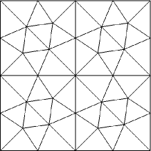
In order to make a numerical convergence study, we have used a family of triangular meshes. These triangle meshes show no symmetry which could artificially increase the convergence rate. This family of meshes is built through the same pattern, which is reproduced at different scales: the first (coarsest) mesh and the third mesh are shown by Figure 4. Although the analytical solution is one-dimensional and the permeability tensor is diagonal, the discrete problem is really 2D because of the non-structured grids. The 2D aspect of the problem is amplified by the choice of a stronger diffusion in the transversal direction.

Figure 4. First and third mesh used in the numerical examples.

For the tests on triangular grids, the final time ${t_{\rm f}}$ has been chosen to $0.25$ and an anisotropic tensor has been consider: $l_{x}=1$ and $l_{y}=10$.

$h$	$\#\mathcal{V}$	${\Delta t}_{\textrm{init}}$	${\Delta t}_{\max}$	$\textrm{err}_{L^{2}}$	rate	$\textrm{err}_{L^{1}}$	rate	$\textrm{err}_{L^{\infty}}$	rate	$u_{\textrm{min}}$	#Newton
0.250	37	0.001	0.01024	0.196E-01	-	0.754E-02	-	0.216E+00	-	0.022	204
0.125	129	0.00025	0.00256	0.512E-02	1.935	0.178E-02	2.084	0.600E-01	1.848	0.004	456
0.063	481	0.00006	0.00064	0.129E-02	1.986	0.430E-03	2.050	0.157E-01	1.931	0.001	1307
0.031	1857	0.00002	0.00016	0.324E-03	1.997	0.107E-03	2.007	0.473E-02	1.734	0.000	3935

Table 1. Triangles. Nonlinear scheme (43).

$h$	$\#\mathcal{V}$	${\Delta t}_{\textrm{init}}$	${\Delta t}_{\max}$	$\textrm{err}_{L^{2}}$	rate	$\textrm{err}_{L^{1}}$	rate	$\textrm{err}_{L^{\infty}}$	rate	$u_{\textrm{min}}$	#Newton
0.250	37	0.001	0.01024	0.187E-01	-	0.708E-02	-	0.225E+00	-	-0.155	33
0.125	129	0.00025	0.00256	0.469E-02	1.993	0.165E-02	2.100	0.786E-01	1.515	-0.046	106
0.063	481	0.00006	0.00064	0.117E-02	1.999	0.406E-03	2.023	0.228E-01	1.784	-0.012	400
0.031	1857	0.00002	0.00016	0.293E-03	1.999	0.102E-03	1.999	0.611E-02	1.901	-0.003	1570

Table 2. Triangles. Linear scheme, fluxes defined by (109).

Let us first observe that the numerical order of convergence is close to 2 for both schemes. The nonlinear scheme is of course more expensive than the linear one but it preserves the positivity of the solution, unlike the linear scheme. This numerical behavior is a verification of the theoretical result mentioned in the Lemma 3.7. In the linear case, the number of Newton-Raphson iterations is equal to the number of time steps. On the finest mesh, the ratio of the number of Newton iterations between the nonlinear and the linear schemes is about $2.5$. It seems to be acceptable in cases where preserving the positivity is mandatory.

Now, in order to exhibit the ability of the VAG scheme to deal with general meshes, the same test case has been applied on a so-called Kershaw grid (cf. Figure 5). Instead of an irrelevant numerical convergence study — it is difficult to define a refinement factor for this type of grids —, we aim to give an evidence that the scheme is free energy diminishing (thus positivity preserving) and that the long-time behavior of the continuous problem is preserved at the discrete level by the scheme. The final time ${t_{\rm f}}$ has been chosen to $250$ and an anisotropic tensor has been consider: $l_{x}=0.001$ and $l_{y}=1$. The results are listed on the Table 3 and we can check again that the nonlinear scheme is positivity preserving despite the irregular grid.

	$\#\mathcal{V}$	${\Delta t}_{\textrm{init}}$	${\Delta t}_{\max}$	$\textrm{err}_{L^{2}}$	$\textrm{err}_{L^{1}}$	$\textrm{err}_{L^{\infty}}$	$u_{\textrm{min}}$	#Newton
nonlinear scheme	324	2.E-04	1	3.99E-02	0.404	1.42E-02	8.92E-04	1148
linear scheme	324	2.E-04	1	3.47E-02	0.377	2.01E-02	-1.49E-02	259

Table 3. Kershaw grid. Nonlinear and linear scheme, with an anisotropic tensor.

Denoting by $w=\pi\exp\left(g(x-\frac{1}{2})\right)$ the long-time asymptotic of ${\widetilde{u}}$ defined by (110), then the relative entropy of a function $u:\Omega\to\mathbb{R}_{+}$ w.r.t. $w$ is defined by

(111) $$E^{w}(u)=\int_{\Omega}\left(u\log\left(\frac{u}{w}\right)-u+w\right){\rm d}{\boldsymbol{x}}.$$

It is simple to verify that

$$\frac{{\rm d}}{{\rm d}t}E^{w}(u)\frac{{\rm d}}{{\rm d}t}E(u)=0.$$

Therefore the decay of the free energy is equivalent to the decay of the relative entropy. Note that $E^{w}$ is undefined (or is set to $+\infty$) if $u<0$ on a positive measure set. It is well known (see e.g. [36, 77]) that the relative entropy $E^{w}({\widetilde{u}}(\cdot,t))$ converges exponentially fast towards $0$ as $t$ tends to $+\infty$. Exponential convergence results in the discrete setting were proved for instance in [39, 38, 17] in the case of a monotone discretization of dissipative equation (see also [16]). In order to check this asymptotic behavior at the discrete level, we introduce the discrete relative entropy $E_{\mathcal{D}}^{w}({\boldsymbol{u}})$ defined for all nonnegative ${\boldsymbol{u}}={(u_{\kappa},u_{\rm s})}_{\kappa,{\rm s}}\in W_{\mathcal{D}}$ (i.e., such that $u_{\beta}\geq 0$ for all $\beta\in\mathcal{M}\cup\mathcal{V}$) by

(112) $$E^{w}_{\mathcal{D}}({\boldsymbol{u}})=\sum_{\beta\in\mathcal{M}\cup\mathcal{V}}m_{\beta}\left(u_{\beta}\log\left(\frac{u_{\beta}}{w({\boldsymbol{x}}_{\beta})}\right)-u_{\beta}+w({\boldsymbol{x}}_{\beta})\right).$$

The exponential convergence towards equilibrium is recovered as it appears clearly on Figure 5.

Figure 5. Left: Kershaw mesh. Right: Evolution of the relative entropy $t\mapsto E^{w}_{\mathcal{D}}({\boldsymbol{u}}(\cdot,t))$ on a logarithmic scale in function of time.

5.2.2. Test 2: Porous medium equation with Dirichlet boundary condition

In this section, we apply our scheme to the case of the anisotropic porous medium equation

(113) $$\partial_{t}u-{\boldsymbol{\nabla}\cdot}\left({\boldsymbol{\Lambda}}\ \boldsymbol{\nabla}(u^{2})\ \right)=0\;\;\text{ in }Q_{t_{\rm f}}$$

for different choices of functions $\eta$ and $p$ with $\int^{u}\eta(a)p^{\prime}(a){\rm d}a=u^{2}$, namely

1. $\eta(u)=2u^{2}$ and $p(u)=\log(u)$,

2. $\eta(u)=2u$ and $p(u)=u$,

3. $\eta(u)=1$ and $p(u)=u^{2}$.

For the choice (a), the function $\eta$ is strictly convex. Therefore, the rigorous gradient flow structure of the problem corresponding to this choice of mobility function $\eta$ is unclear [43]. The pressure function $p$ is singular near $0$, hence Lemma 3.7 implies that the corresponding scheme is positivity preserving.

The choice (b) with a linear mobility corresponds to the now classical setting highlighted in [86, 77].

Finally, the choice (c) corresponds to the usual approach for discretizing the porous medium equation. The corresponding scheme enters into the framework of [48], where its convergence is proved.

The problem is closed here with Dirichlet boundary conditions (destroying by the way the gradient flow structure but not the convergence of the scheme).

Comparison with a one-dimensional analytical solution. The numerical convergence of the three schemes has first been compared thanks to the following analytical solution (again built in $1$-dimension),

(114) $$\widehat{u}(x,y,t)=\max\left(2l_{x}t-x\ ,\ 0\right),\quad\forall((x,y),t)\in Q_{t_{\rm f}}.$$

Note that (114) is the unique weak solution corresponding to the initial condition $u_{0}(x,y)=\widehat{u}(x,y,0)$ and to the Dirichlet boundary condition $u_{D}(x,y,t)=\widehat{u}(x,y,t)$ on $\partial\Omega\times(0,{t_{\rm f}})$. Our numerical convergence study makes use of the family of triangular meshes already used for Test 1. Once again, the final time ${t_{\rm f}}$ is fixed to $0.25$ and an anisotropic tensor is given by $l_{x}=1$ and $l_{y}=10$.

$h$	$\#\mathcal{V}$	${\Delta t}_{\textrm{init}}$	${\Delta t}_{\max}$	$\textrm{err}_{L^{2}}$	rate	$\textrm{err}_{L^{1}}$	rate	$\textrm{err}_{L^{\infty}}$	rate	$u_{\textrm{min}}$	#Newton
0.306	37	0.001	0.01024	0.523E-02	-	0.997E-03	-	0.105E+00	-	0.000	479
0.153	129	0.00025	0.00256	0.205E-02	1.352	0.344E-03	1.535	0.522E-01	1.013	0.000	1143
0.077	481	0.00006	0.00064	0.898E-03	1.190	0.123E-03	1.490	0.259E-01	1.012	0.000	2218
0.038	1857	0.00002	0.00016	0.380E-03	1.240	0.417E-04	1.554	0.128E-01	1.012	0.000	5652

Table 4. Test 2: Choice (a) of mobility and pressure functions, convergence towards (114).

$h$	$\#\mathcal{V}$	${\Delta t}_{\textrm{init}}$	${\Delta t}_{\max}$	$\textrm{err}_{L^{2}}$	rate	$\textrm{err}_{L^{1}}$	rate	$\textrm{err}_{L^{\infty}}$	rate	$u_{\textrm{min}}$	#Newton
0.306	37	0.001	0.01024	0.769E-02	-	0.210E-02	-	0.645E-01	-	-0.032	138
0.153	129	0.00025	0.00256	0.263E-02	1.546	0.613E-03	1.775	0.326E-01	0.983	-0.017	383
0.077	481	0.00006	0.00064	0.897E-03	1.554	0.173E-03	1.823	0.164E-01	0.996	-0.009	1246
0.038	1857	0.00002	0.00016	0.306E-03	1.551	0.481E-04	1.849	0.821E-02	0.996	-0.005	4234

Table 5. Test 2: Choice (b) of mobility and pressure functions, convergence towards (114).

$h$	$\#\mathcal{V}$	${\Delta t}_{\textrm{init}}$	${\Delta t}_{\max}$	$\textrm{err}_{L^{2}}$	rate	$\textrm{err}_{L^{1}}$	rate	$\textrm{err}_{L^{\infty}}$	rate	$u_{\textrm{min}}$	#Newton
0.306	37	0.001	0.01024	0.116E-01	-	0.371E-02	-	0.764E-01	-	-0.065	148
0.153	129	0.00025	0.00256	0.423E-02	1.461	0.116E-02	1.672	0.388E-01	0.977	-0.039	436
0.077	481	0.00006	0.00064	0.149E-02	1.501	0.337E-03	1.788	0.233E-01	0.737	-0.021	1438
0.038	1857	0.00002	0.00016	0.524E-03	1.513	0.932E-04	1.856	0.129E-01	0.856	-0.010	4912

Table 6. Test 2: Choice (c) of mobility and pressure functions, convergence towards (114).

We observe in Tables 4–6 that second order convergence is destroyed for all the three schemes because of the lack of regularity of the exact solution. As expected, the discrete solution corresponding to the choice (a) remains positive while the discrete solutions to the schemes corresponding to the choices (b) and (c) suffer of undershoots. The choice (b) appears to be both cheaper and more accurate than the choice (c), and the amplitude of the undershoots is smaller.

Figure 6. Test 2. Coarsest grid. Discrete unknown $(u_{{\rm s}})_{{\rm s}\in\mathcal{V}_{\kappa}}$ and its iso-values. Choice (a) (left) and (c) (right) for $\eta$ and $p$.

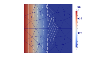
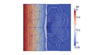
Figure 6 illustrates the iso-values of the piecewise affine functions defined on the triangular mesh $\mathcal{M}$ reconstructed thanks to its nodal values $\left(u_{\rm s}^{n}\right)_{{\rm s}\in\mathcal{V}}$ for the coarsest triangle grid at the final time ${t_{\rm f}}$. For the choice (a) of the mobility and the pressure (left), the iso-values are chosen from $0$ to $0.025$ by step of $0.05$ and then from $0.1$ to $0.5$ by step of $0.1$. For the choice (c) of the mobility and the pressure (right), the iso-values are taken from $-0.025$ to $0.025$ by step of $0.05$ and also from $0.1$ to $0.5$ by step of $0.1$.

Comparison with a two-dimensional analytical solution. We test our approach on the two-dimensional analytical solution

(115) $$\widehat{u}(x,y,t)=\dfrac{\alpha(x-0.5)^{2}+\beta(y-0.5)^{2}}{1-t}\qquad\mathrm{in}\;Q_{t_{\rm f}}$$

of the anisotropic porous medium equation (113), where ${t_{\rm f}}$ has been set to 0.25. The permeability tensor is still assumed to be diagonal with $l_{x}=0.1$ and $l_{y}=10$, and we have set $\alpha=\frac{1}{16l_{x}}$ and $\beta=\frac{1}{16l_{y}}$. The problem is closed with Dirichlet boundary conditions and the initial condition corresponding to (115). The results are gathered in Tables 7–9.

$h$	$\#\mathcal{V}$	${\Delta t}_{\textrm{init}}$	${\Delta t}_{\max}$	$\textrm{err}_{L^{2}}$	rate	$\textrm{err}_{L^{1}}$	rate	$\textrm{err}_{L^{\infty}}$	rate	$u_{\textrm{min}}$	#Newton
0.306	37	0.001	0.01024	0.270E-02	-	0.114E-02	-	0.120E-01	-	0.000	89
0.153	129	0.00025	0.00256	0.942E-03	1.517	0.381E-03	1.578	0.473E-02	1.341	0.000	223
0.077	481	0.00006	0.00064	0.293E-03	1.688	0.119E-03	1.686	0.163E-02	1.534	0.000	805
0.038	1857	0.00002	0.00016	0.802E-04	1.868	0.334E-04	1.828	0.461E-03	1.826	0.000	3142

Table 7. Test 2: Choice (a) of mobility and pressure functions, convergence towards (115).

$h$	$\#\mathcal{V}$	${\Delta t}_{\textrm{init}}$	${\Delta t}_{\max}$	$\textrm{err}_{L^{2}}$	rate	$\textrm{err}_{L^{1}}$	rate	$\textrm{err}_{L^{\infty}}$	rate	$u_{\textrm{min}}$	#Newton
0.306	37	0.001	0.01024	0.645E-02	-	0.271E-02	-	0.271E-01	-	-0.027	99
0.153	129	0.00025	0.00256	0.202E-02	1.676	0.828E-03	1.709	0.992E-02	1.447	-0.008	237
0.077	481	0.00006	0.00064	0.604E-03	1.742	0.246E-03	1.753	0.341E-02	1.540	-0.002	801
0.038	1857	0.00002	0.00016	0.161E-03	1.905	0.667E-04	1.882	0.966E-03	1.821	0.000	3140

Table 8. Test 2: Choice (b) of mobility and pressure functions, convergence towards (115).

$h$	$\#\mathcal{V}$	${\Delta t}_{\textrm{init}}$	${\Delta t}_{\max}$	$\textrm{err}_{L^{2}}$	rate	$\textrm{err}_{L^{1}}$	rate	$\textrm{err}_{L^{\infty}}$	rate	$u_{\textrm{min}}$	#Newton
0.306	37	0.001	0.01024	0.102E-01	-	0.448E-02	-	0.575E-01	-	-0.046	128
0.153	129	0.00025	0.00256	0.321E-02	1.661	0.134E-02	1.739	0.194E-01	1.569	-0.011	250
0.077	481	0.00006	0.00064	0.933E-03	1.783	0.383E-03	1.811	0.553E-02	1.808	-0.003	810
0.038	1857	0.00002	0.00016	0.244E-03	1.933	0.101E-03	1.927	0.147E-02	1.914	-0.001	3140

Table 9. Test 2. Choice (c) of mobility and pressure functions, convergence towards (115).

As expected, the choice (a) leads to a positivity preserving scheme, contrarily to the choices (b) and (c). Moreover, the scheme (a) is the most accurate and does not come with an additional cost.

5.2.3. Test 3: Porous medium equation with drift

In this third test case, we have set $\eta(u)=u$ on $\mathbb{R}_{+}$ and $p(u)=2u$ and $g=1$, leading to the degenerate problem

(116) $$\partial_{t}u-{\boldsymbol{\nabla}\cdot}\left({\boldsymbol{\Lambda}}\ (\boldsymbol{\nabla}(u^{2})-u{\mathbf{g}})\ \right)=0\;\;\text{ in }Q_{t_{\rm f}}.$$

The problem is endowed with Dirichlet boundary conditions. The tensor ${\boldsymbol{\Lambda}}$ is chosen to be diagonal with $l_{x}=1$ and $l_{y}=100$. We compare the results obtained by (43) with those obtained using, instead of (43c), this particular definition of the fluxes

(117) $$\widehat{F}_{\kappa,{\rm s}}({\boldsymbol{u}}^{n})=\sum_{{\rm s}^{\prime}\in\mathcal{V}_{\kappa}}a^{\kappa}_{{\rm s},{\rm s}^{\prime}}((u_{\kappa}^{n})^{2}-(u_{{\rm s}^{\prime}}^{n})^{2})+\frac{u_{\kappa}^{n}+u_{\rm s}^{n}}{2}\sum_{{\rm s}^{\prime}\in\mathcal{V}_{\kappa}}a^{\kappa}_{{\rm s},{\rm s}^{\prime}}(V_{\kappa}-V_{{\rm s}^{\prime}}),\\ \quad\forall\kappa\in\mathcal{M},\;\forall{\rm s}\in\mathcal{V}_{\kappa}.$$

The resulting scheme is called the quasilinear scheme. The numerical convergence of both schemes has been compared on the sequence of triangular meshes already used in the previous tests, thanks to the following analytical solution (again built in $1$-dimension),

(118) $$\widehat{u}(x,y,t)=\max\left(\beta t-x\ ,\ 0\right),\quad\forall((x,y),t)\in\Omega\times(0,{t_{\rm f}}),$$

with $\beta=l_{x}(2+g)$. The profile (118) is the unique weak solution corresponding to the initial condition $u_{0}(x,y)=\widehat{u}(x,y,0)$ in $\Omega$ and the Dirichlet boundary condition $u_{D}(x,y,t)=\widehat{u}(x,y,t)$ on $\partial\Omega\times(0,{t_{\rm f}})$.

$h$	$\#\mathcal{V}$	${\Delta t}_{\textrm{init}}$	${\Delta t}_{\max}$	$\textrm{err}_{L^{2}}$	rate	$\textrm{err}_{L^{1}}$	rate	$\textrm{err}_{L^{\infty}}$	rate	$u_{\textrm{min}}$	#Newton
0.306	37	0.001	0.01024	0.130E-01	-	0.423E-02	-	0.890E-01	-	-0.046	187
0.153	129	0.00025	0.00256	0.495E-02	1.398	0.133E-02	1.675	0.496E-01	0.843	-0.032	552
0.077	481	0.00006	0.00064	0.184E-02	1.428	0.397E-03	1.741	0.283E-01	0.808	-0.017	1609
0.038	1857	0.00002	0.00016	0.660E-03	1.479	0.116E-03	1.771	0.145E-01	0.970	-0.009	5586

Table 10. Test 3. Nonlinear scheme (43).

$h$	$\#\mathcal{V}$	${\Delta t}_{\textrm{init}}$	${\Delta t}_{\max}$	$\textrm{err}_{L^{2}}$	rate	$\textrm{err}_{L^{1}}$	rate	$\textrm{err}_{L^{\infty}}$	rate	$u_{\textrm{min}}$	#Newton
0.306	37	0.001	0.01024	0.154E-01	-	0.568E-02	-	0.939E-01	-	-0.068	193
0.153	129	0.00025	0.00256	0.671E-02	1.201	0.213E-02	1.416	0.613E-01	0.615	-0.048	642
0.077	481	0.00006	0.00064	0.271E-02	1.309	0.702E-03	1.600	0.326E-01	0.910	-0.027	2178
0.038	1857	0.00002	0.00016	0.104E-02	1.384	0.212E-03	1.725	0.170E-01	0.938	-0.015	7365

Table 11. Test 3. Quasilinear scheme, fluxes defined by (117).

Here again, the convergence orders of both scheme are similar, but strictly lower than $2$ because of the lack of regularity of the exact solution. Both schemes violate the positivity of the solution in this case, but the amplitude of the undershoots is smaller for the nonlinear scheme. There is no contradiction here with Lemma 3.7 since $p$ is not singular at $u=0$. Our nonlinear scheme is slightly more accurate, produces undershoots with a smaller amplitude, and is cheaper than the quasilinear one.

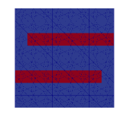
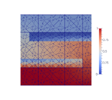
5.2.4. Test 4. A heterogeneous test case

The last test aims to illustrate the ability of the scheme to deal with heterogeneous situations. Motivated by an application to complex flows in porous media (see for instance [35, 32]), we test the nonlinear VAG scheme in a slightly more complicated configuration where both the permeability tensor ${\boldsymbol{\Lambda}}$ and the pressure function $p$ depend on ${\boldsymbol{x}}$ in a discontinuous way. More precisely, the domain $\Omega=(0,1)^{2}$ is made of two open subdomains $\Omega_{1}$ (the drain) and $\Omega_{2}$ (the barrier) with ${\overline{\Omega}}={\overline{\Omega}}_{1}\cup{\overline{\Omega}}_{2}$ and $\Omega_{1}\cap\Omega_{2}=\emptyset$ (see Figure 7 for a representation of $\Omega_{1}$ and $\Omega_{2}$). The permeability tensor and the pressure function are defined by

$${\boldsymbol{\Lambda}}({\boldsymbol{x}})=\begin{cases}{\boldsymbol{\Lambda}}_{1}={\bf I}_{d}&\text{if}\;{\boldsymbol{x}}\in\Omega_{1},\\ {\boldsymbol{\Lambda}}_{2}=\begin{pmatrix}1&0\\ 0&0.01\end{pmatrix}&\text{if}\;{\boldsymbol{x}}\in\Omega_{2},\\ \end{cases}$$

and

$$p(u,{\boldsymbol{x}})=\begin{cases}p_{1}(u)=3\log(u)&\text{if}\;{\boldsymbol{x}}\in\Omega_{1},\\ p_{2}(u)=\log(u)&\text{if}\;{\boldsymbol{x}}\in\Omega_{2}.\end{cases}$$

The mobility function is linear and does not depend on ${\boldsymbol{x}}$, i.e., $\eta(u)=u$. For the sake of simplicity, we have set $V=0$. At the interface $J$ between $\Omega_{1}$ and $\Omega_{2}$, the flux and the pressure are assumed to be continuous, i.e., denoting by $u_{i}$ the restriction of $u$ to $\Omega_{i}$ and by ${{\boldsymbol{n}}}_{i}$ the normal to $J$ outward w.r.t. $\Omega_{i}$, we require

(119) $$3{\boldsymbol{\Lambda}}_{1}\boldsymbol{\nabla}u_{1}\cdot{{\boldsymbol{n}}}_{1}+{\boldsymbol{\Lambda}}_{2}\boldsymbol{\nabla}u_{2}\cdot{\boldsymbol{n}}_{2}=0,\quad\text{and}\quad p_{1}(u_{1})=p_{2}(u_{2})\quad\text{on}\;J\times(0,{t_{\rm f}}).$$

The problem is complemented with the boundary conditions

• $p(u,{\boldsymbol{x}})=0$ (hence $u=1$) on the bottom boundary,

• $p(u,{\boldsymbol{x}})=-4$ (hence $u\simeq 0.018$) on the top boundary,

• ${\boldsymbol{\Lambda}}\boldsymbol{\nabla}u\cdot{\boldsymbol{n}}=0$ on the lateral boundaries.

The initial data is chosen at equilibrium, with $p(u_{0},{\boldsymbol{x}})=-4$ in the whole $\Omega$. Existence and uniqueness for this problem follow from the analysis carried out in [28].

Since $u$ is discontinuous across $J$ (in opposition to the pressure $p(u,\cdot)$ following (119)), it is natural to choose $p$ rather than $u$ as the primary variable of the numerical scheme (cf. [62, 55], we refer to [23] for an alternate strategy that improves robustness) in order to avoid the complex treatment of the jump condition (119) at the interface performed for instance in [28, 29, 47, 24].

The mesh $\mathcal{M}$ is assumed to be compatible with the geometry of $\Omega$, in the sense that $\kappa\in\mathcal{M}$ is either contained in $\Omega_{1}$ or $\Omega_{2}$, but $J\cap\kappa=\emptyset$ for all $\kappa\in\mathcal{M}$ (cf. Figure 7). Define the functions $u_{\kappa}:\mathbb{R}\to(0,\infty)$ as the inverse of $p(\cdot,{\boldsymbol{x}}_{\kappa})$ for all $\kappa\in\mathcal{M}$. The subset of $\mathcal{V}$ made of vertices belonging to the top or bottom boundaries where Dirichlet boundary conditions hold is denoted by $\mathcal{V}_{\rm ext}$. We also make use of the notations $\mathcal{V}_{\rm int}=\mathcal{V}\setminus\mathcal{V}_{\rm ext}$ and $\mathcal{V}_{\kappa,\rm int}=\mathcal{V}_{\rm int}\cap\mathcal{V}_{\kappa}$ for $\kappa\in\mathcal{M}$. The scheme (43) expressed with $p$ as a primary variable consists in finding $\boldsymbol{p}=\left(p_{\kappa}^{n},p_{\rm s}^{n}\right)_{\kappa,{\rm s},n}$ in $W_{\mathcal{D},{\boldsymbol{\Delta}t}}$ such that for all $n\geq 1$,

$$\left\{\begin{array}[]{ll}\displaystyle\frac{u_{\kappa}(p_{\kappa}^{n})-u_{\kappa}(p_{\kappa}^{n-1})}{{\Delta t}_{n}}m_{\kappa}+\sum_{{\rm s}\in\mathcal{V}_{\kappa}}F_{\kappa,{\rm s}}^{n}=0,&\forall\kappa\in\mathcal{M},\\[5.0pt] \displaystyle\sum_{\kappa\in\mathcal{M}_{\rm s}}\frac{u_{\kappa}(p_{\rm s}^{n})-u_{\kappa}(p_{\rm s}^{n-1})}{{\Delta t}_{n}}m_{\kappa,{\rm s}}+\sum_{\kappa\in\mathcal{M}_{\rm s}}F_{{\rm s},\kappa}^{n}=0,&\forall{\rm s}\in\mathcal{V}_{\rm int},\\[5.0pt] F_{\kappa,{\rm s}}^{n}+F_{{\rm s},\kappa}^{n}=0,&\forall\kappa\in\mathcal{M},\forall{\rm s}\in\mathcal{V}_{\kappa,\rm int},\\[5.0pt] \displaystyle F_{\kappa,{\rm s}}^{n}=\sqrt{\eta_{\kappa,{\rm s}}^{n}}\sum_{{\rm s}^{\prime}\in\mathcal{V}_{\kappa}}a_{{\rm s},{\rm s}^{\prime}}^{\kappa}\sqrt{\eta_{\kappa,{\rm s}^{\prime}}^{n}}(p_{\kappa}^{n}-p_{{\rm s}^{\prime}}^{n}),&\forall\kappa\in\mathcal{M},\;\forall{\rm s}\in\mathcal{V}_{\kappa},\\[5.0pt] \displaystyle\eta_{\kappa,{\rm s}}^{n}={\frac{u_{\kappa}(p_{\kappa}^{n})+u_{\kappa}(p_{\rm s}^{n})}{2}},&\forall\kappa\in\mathcal{M},\,\forall{\rm s}\in\mathcal{V}_{\kappa}.\end{array}\right.$$

Figure 7. Test 4. Illustration of the two sub-domains: the drain $\Omega_{1}$ in blue and the barriers $\Omega_{2}$ in red. Left: cartesian grid. Right: unstructured triangular grid.

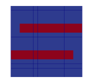
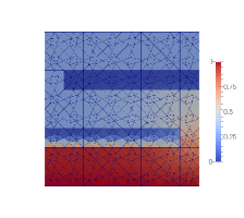
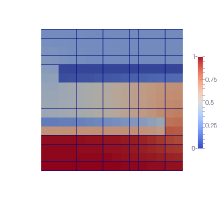
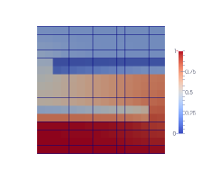
We observe on Figure 8 that the results on the triangular mesh (with $481$ nodes) and on the cartesian mesh (with $289$ nodes) are similar. Moreover, the numbers of Newton-Raphson iteration needed to compute both solutions are of the same order.

(a)

(b)

(c)

(d)

(e)

(f)

Figure 8. Approximation of $u(p,{\boldsymbol{x}})$ at times $t=0.05$, $t=0.2$, and $t=1$ for the two different meshes.

Appendix A Some lemmas related to the VAG discretization

This appendix gathers lemmas on some properties of the VAG discretization that are independent of the continuous problem (and thus of the scheme). In what follows, $\mathcal{D}=(\mathcal{M},\mathcal{T})$ denote a discretization of $\Omega$ as prescribed in §2.1.1, and $\pi_{\mathcal{T}},\pi_{\mathcal{M}},\pi_{\mathcal{D}}$ and $\boldsymbol{\nabla}_{\mathcal{T}}$ are the corresponding reconstruction operators.

Lemma A.1.

For $\kappa\in\mathcal{M}$, let ${\bf A}_{\kappa}=\left(a^{\kappa}_{{\rm s},{\rm s}^{\prime}}\right)_{{\rm s},{\rm s}^{\prime}\in\mathcal{V}_{\kappa}}$ be the matrix defined by (34), then there exists $C$ depending only on ${\boldsymbol{\Lambda}}$, $\theta_{\mathcal{T}}$ and $\ell_{\mathcal{D}}$ (but not on $\kappa$) such that ${\rm Cond}_{2}({\bf A}_{\kappa})\leq C$.

Proof.

Following [26, Lemma 3.2], there exist $C_{1},C_{2}>0$ depending only on $\theta_{\mathcal{T}}$ and $\ell_{\mathcal{D}}$ such that, for all ${\boldsymbol{u}}\in W_{\mathcal{D}}$ and all $\kappa\in\mathcal{M}$, one has

$$C_{1}\frac{{\rm meas}(\kappa)}{(h_{\kappa})^{2}}\sum_{{\rm s}\in\mathcal{V}_{\kappa}}\left(u_{\rm s}-u_{\kappa}\right)^{2}\leq{\|\boldsymbol{\nabla}_{\mathcal{T}}{\boldsymbol{u}}\|}^{2}_{L^{2}(\kappa)}\leq C_{2}\frac{{\rm meas}(\kappa)}{(h_{\kappa})^{2}}\sum_{{\rm s}\in\mathcal{V}_{\kappa}}\left(u_{\rm s}-u_{\kappa}\right)^{2},$$

where $h_{\kappa}$ denotes the diameter of the cell $\kappa\in\mathcal{M}$. As a consequence, one has

$$\lambda_{\star}C_{1}\frac{{\rm meas}(\kappa)}{(h_{\kappa})^{2}}|{\boldsymbol{\delta}}_{\kappa}{\boldsymbol{u}}|^{2}\leq{\boldsymbol{\delta}}_{\kappa}{\boldsymbol{u}}\cdot{\bf A}_{\kappa}{\boldsymbol{\delta}}_{\kappa}{\boldsymbol{u}}=\int_{\kappa}{\boldsymbol{\Lambda}}\boldsymbol{\nabla}_{\mathcal{T}}{\boldsymbol{u}}\cdot\boldsymbol{\nabla}_{\mathcal{T}}{\boldsymbol{u}}\,{\rm d}{\boldsymbol{x}}\leq\lambda^{\star}C_{2}\frac{{\rm meas}(\kappa)}{(h_{\kappa})^{2}}|{\boldsymbol{\delta}}_{\kappa}{\boldsymbol{u}}|^{2}.$$

Since the application ${\boldsymbol{\delta}}_{\kappa}:W_{\mathcal{D}}\to\mathbb{R}^{\ell_{\kappa}}$ is onto, we deduce that

$$\lambda_{\star}C_{1}\frac{{\rm meas}(\kappa)}{(h_{\kappa})^{2}}|{\boldsymbol{v}}|^{2}\leq{\boldsymbol{v}}\cdot{\bf A}_{\kappa}{\boldsymbol{v}}\leq\lambda^{\star}C_{2}\frac{{\rm meas}(\kappa)}{(h_{\kappa})^{2}}|{\boldsymbol{v}}|^{2},\qquad\forall{\boldsymbol{v}}\in\mathbb{R}^{\ell_{\kappa}},$$

and thus that ${\rm Cond}_{2}({\bf A}_{\kappa})\leq\frac{\lambda^{\star}C_{2}}{\lambda_{\star}C_{1}}.$ ∎

Lemma A.2.

There exists $C\geq 1$ depending only on ${\boldsymbol{\Lambda}}$, $\theta_{\mathcal{T}}$ and $\ell_{\mathcal{D}}$ such that, for all $\kappa\in\mathcal{M}$ and all ${\boldsymbol{v}}={(v_{\rm s})}_{{\rm s}\in\mathcal{V}_{\kappa}}\in\mathbb{R}^{\ell_{\kappa}}$, one has

$$\sum_{{\rm s}\in\mathcal{V}_{\kappa}}\left(\sum_{{\rm s}^{\prime}\in\mathcal{V}_{\kappa}}|a^{\kappa}_{{\rm s},{\rm s}^{\prime}}|\right)\left(v_{\rm s}\right)^{2}\leq C\;{\boldsymbol{v}}\cdot{\bf A}_{\kappa}{\boldsymbol{v}}.$$

Proof.

Denoting by $\|\cdot\|_{q}$ the usual matrix $q$-norm, one has

$$\sum_{{\rm s}\in\mathcal{V}_{\kappa}}\left(\sum_{{\rm s}^{\prime}\in\mathcal{V}_{\kappa}}|a^{\kappa}_{{\rm s},{\rm s}^{\prime}}|\right)\left(v_{\rm s}\right)^{2}\leq{\|{\bf A}_{\kappa}\|}_{1}|{\boldsymbol{v}}|^{2}.$$

Since the dimension of the space $\mathbb{R}^{\ell_{\kappa}}$ is bounded by $\ell_{\mathcal{D}}$, there exists $C_{1}$ depending only on $\ell_{\mathcal{D}}$ such that $\|{\bf A}_{\kappa}\|_{1}\leq C_{1}\|{\bf A}_{\kappa}\|_{2}$, so that

(120) $$\sum_{{\rm s}\in\mathcal{V}_{\kappa}}\left(\sum_{{\rm s}^{\prime}\in\mathcal{V}_{\kappa}}|a^{\kappa}_{{\rm s},{\rm s}^{\prime}}|\right)\left(v_{\rm s}\right)^{2}\leq C_{1}{\|{\bf A}_{\kappa}\|}_{2}|{\boldsymbol{v}}|^{2}.$$

On the other hand, since ${\bf A}_{\kappa}$ is symmetric definite and positive, one has

$${\boldsymbol{v}}\cdot{\bf A}_{\kappa}{\boldsymbol{v}}\geq\frac{{\|{\bf A}_{\kappa}\|}_{2}}{{\rm Cond}_{2}({\bf A}_{\kappa})}|{\boldsymbol{v}}|^{2}.$$

Using Lemma A.1, we obtain that there exists $C_{2}>0$ depending only on ${\boldsymbol{\Lambda}}$, $\theta_{\mathcal{T}}$ and $\ell_{\mathcal{D}}$ such that

(121) $${\boldsymbol{v}}\cdot{\bf A}_{\kappa}{\boldsymbol{v}}\geq C_{2}{{\|{\bf A}_{\kappa}\|}_{2}}|{\boldsymbol{v}}|^{2}.$$

Putting (120) and (121) together, we conclude the proof of Lemma A.2 by choosing $C=\frac{C_{1}}{C_{2}}$. ∎

Lemma A.3.

Let $\kappa\in\mathcal{M}$ and ${\bf A}_{\kappa}=(a^{\kappa}_{{\rm s},{\rm s}^{\prime}})_{{\rm s},{\rm s}^{\prime}\in\mathcal{V}_{\kappa}}\in\mathbb{R}^{\ell_{\kappa}\times\ell_{\kappa}}$ be the matrix defined by (34). Let ${\boldsymbol{\mu}}_{\kappa}=\left(\mu_{\kappa,{\rm s}}\right)_{{\rm s}\in\mathcal{V}_{\kappa}}\in\mathbb{R}^{\ell_{\kappa}}$ and ${\boldsymbol{v}}\in W_{\mathcal{D}}$, then

$$\sum_{{\rm s}\in\mathcal{V}_{\kappa}}\sum_{{\rm s}^{\prime}\in\mathcal{V}_{\kappa}}(v_{\rm s}-v_{\kappa})\mu_{\kappa,{\rm s}}a^{\kappa}_{{\rm s},{\rm s}^{\prime}}\mu_{\kappa,{\rm s}^{\prime}}(v_{{\rm s}^{\prime}}-v_{\kappa})\leq\max_{{\rm s}\in\mathcal{V}_{\kappa}}(\mu_{\kappa,{\rm s}})^{2}\sum_{{\rm s}\in\mathcal{V}_{\kappa}}\left(\sum_{{\rm s}^{\prime}\in\mathcal{V}_{\kappa}}|a^{\kappa}_{{\rm s},{\rm s}^{\prime}}|\right)\left(v_{\rm s}-v_{\kappa}\right)^{2}.$$

Proof.

Using $ab\leq\frac{a^{2}}{2}+\frac{b^{2}}{2}$, we obtain that

$$\sum_{{\rm s}\in\mathcal{V}_{\kappa}}\sum_{{\rm s}^{\prime}\in\mathcal{V}_{\kappa}}(v_{\rm s}-v_{\kappa})\mu_{\kappa,{\rm s}}a^{\kappa}_{{\rm s},{\rm s}^{\prime}}\mu_{\kappa,{\rm s}^{\prime}}(v_{{\rm s}^{\prime}}-v_{\kappa})\\ \leq\max_{{\rm s}\in\mathcal{V}_{\kappa}}(\mu_{\kappa,{\rm s}})^{2}\sum_{{\rm s}\in\mathcal{V}_{\kappa}}\sum_{{\rm s}^{\prime}\in\mathcal{V}_{\kappa}}|v_{\rm s}-v_{\kappa}||a^{\kappa}_{{\rm s},{\rm s}^{\prime}}||v_{{\rm s}^{\prime}}-v_{\kappa}|\\ \leq\frac{\max_{{\rm s}\in\mathcal{V}_{\kappa}}(\mu_{\kappa,{\rm s}})^{2}}{2}\sum_{{\rm s}\in\mathcal{V}_{\kappa}}\left(\sum_{{\rm s}^{\prime}\in\mathcal{V}_{\kappa}}|a^{\kappa}_{{\rm s},{\rm s}^{\prime}}|\right)(v_{\rm s}-v_{\kappa})^{2}\\ +\frac{\max_{{\rm s}\in\mathcal{V}_{\kappa}}(\mu_{\kappa,{\rm s}})^{2}}{2}\sum_{{\rm s}^{\prime}\in\mathcal{V}_{\kappa}}\left(\sum_{{\rm s}\in\mathcal{V}_{\kappa}}|a^{\kappa}_{{\rm s},{\rm s}^{\prime}}|\right)(v_{\rm s}^{\prime}-v_{\kappa})^{2}.$$

One concludes the proof of Lemma A.3 by noticing that, since ${\bf A}_{\kappa}$ is symmetric, the two terms in the right-hand side of the above inequality are equal. ∎

Lemma A.4.

There exists $C$ depending only on $\theta_{\mathcal{T}}$ and $\ell_{\mathcal{D}}$ such that

$${\rm meas}(T)\leq{\rm meas}(\kappa)\leq C{\rm meas}(T),\qquad\forall\kappa\in\mathcal{M},\;\forall T\in\mathcal{T}\text{with }T\subset\kappa.$$

Proof.

Let $\kappa\in\mathcal{M}$, then there exist $T_{1},\dots,T_{r}$ simplexes, with $r=\ell_{\kappa}$ if $d=2$ and $r=2\#\mathcal{E}_{\kappa}$ if $d=3$, such that

$$\bigcup_{i=1}^{r_{\kappa}}{\overline{T}}_{i}={\overline{\kappa}},\qquad T_{i}\cap T_{j}=\emptyset\;\text{if }\;i\neq j.$$

The Euler-Descartes theorem ensures that $r\leq 4(\ell_{\mathcal{D}}-1)$ if $d=3$.

If $T_{i}$ and $T_{j}$ share a common edge, one gets that

$${\rm meas}(T_{i})\leq\theta^{d}\;{\rm meas}(T_{j}).$$

Let $i_{0},i_{1}\in\{1,\dots,r_{\kappa}\}$ be arbitrary but different, we deduce from the previous inequality the following non-optimal estimate:

$${\rm meas}(T_{i_{0}})\leq\theta^{4(\ell_{\mathcal{D}}-1)d}\;{\rm meas}(T_{i_{1}}).$$

Let $i_{\rm max}$ be such that ${\rm meas}(T_{i_{\rm max}})=\max_{1\leq i\leq r}{\rm meas}(T_{i})$, then

$${\rm meas}(\kappa)\leq r\;{\rm meas}(T_{i_{\rm max}})\leq 4(\ell_{\mathcal{D}}-1)\theta^{4(\ell_{\mathcal{D}}-1)d}{\rm meas}(T_{i}),\qquad\forall i\in\{1,\dots,r\}.$$

∎

We state now a slight generalization of [26, Lemma 3.4], where the same result is proven in the particular case $q=2$. The straightforward adaptation of the proof given in [26] to the case $q\neq 2$ is left to the reader.

Lemma A.5.

There exists $C$ depending only on $\ell_{\mathcal{D}}$ and $\theta_{\mathcal{T}}$ defined in (24) and (21) respectively such that, for all ${\boldsymbol{v}}\in W_{\mathcal{D}}$ and all $q\in[1,\infty]$, one has

$$\left\|\pi_{\mathcal{D}}{\boldsymbol{v}}-\pi_{\mathcal{T}}{\boldsymbol{v}}\right\|_{L^{q}(\Omega)}+\left\|\pi_{\mathcal{D}}{\boldsymbol{v}}-\pi_{\mathcal{M}}{\boldsymbol{v}}\right\|_{L^{q}(\Omega)}\leq Ch_{\mathcal{T}}\left\|\boldsymbol{\nabla}_{\mathcal{T}}{\boldsymbol{v}}\right\|_{L^{q}(\Omega)}.$$

Lemma A.6.

Let $\mathcal{D}$ be a discretization of $\Omega$ as introduced in §2.1.1 such that $\zeta_{\mathcal{D}}>0$, then there exist $C_{1}>0$ depending only on $q$, $\theta_{\mathcal{T}}$ and $\ell_{\mathcal{D}}$ and $C_{2}$ depending moreover on $\zeta_{\mathcal{D}}$ such that

(122) $$C_{1}\|\pi_{\mathcal{D}}{\boldsymbol{v}}\|_{L^{q}(\Omega)}\leq\|\pi_{\mathcal{T}}{\boldsymbol{v}}\|_{L^{q}(\Omega)}\leq C_{2}\|\pi_{\mathcal{D}}{\boldsymbol{v}}\|_{L^{q}(\Omega)},\qquad\forall{\boldsymbol{v}}\in W_{\mathcal{D}}.$$

Proof.

Let ${\widehat{T}}$ be a reference tetrahedron, and let ${\widehat{v}}:{\widehat{T}}\to\mathbb{R}$ be an affine function with nodal values $v_{i}$, $i\in\{1,\dots 4\}$, then for all $q>0$, there exists $C$ depending on $q$ such that

$$\frac{1}{C}\sum_{i=1}^{4}|v_{i}|^{q}\leq\|{\widehat{v}}\|_{L^{q}({\widehat{T}})}^{q}\leq C\sum_{i=1}^{4}|v_{i}|^{q}.$$

Therefore, using classical properties of the affine change of variable between simplexes, one gets the existence of $C$ depending only on $q$, $\theta_{\mathcal{T}}$, and $\ell_{\mathcal{D}}$ such that, for all ${\boldsymbol{v}}\in W_{\mathcal{D}}$,

(123) $$\frac{1}{C}\sum_{\kappa\in\mathcal{M}}{\rm meas}(\kappa)\left(|v_{\kappa}|^{q}+\sum_{{\rm s}\in\mathcal{V}_{\kappa}}|v_{\rm s}|^{q}\right)\\ \leq\|\pi_{\mathcal{T}}{\boldsymbol{v}}\|_{L^{q}(\Omega)}^{q}\leq C\sum_{\kappa\in\mathcal{M}}{\rm meas}(\kappa)\left(|v_{\kappa}|^{q}+\sum_{{\rm s}\in\mathcal{V}_{\kappa}}|v_{\rm s}|^{q}\right).$$

On the other hand, one has

$$\|\pi_{\mathcal{D}}{\boldsymbol{v}}\|_{L^{q}(\Omega)}^{q}=\sum_{\kappa\in\mathcal{M}}m_{\kappa}|v_{\kappa}|^{q}+\sum_{{\rm s}\in\mathcal{V}}m_{\rm s}|v_{\rm s}|^{q}.$$

A classical geometrical property and (29) yield

(124) $$m_{\kappa}\leq{\rm meas}(\kappa)=d\int_{\Omega}\pi_{\mathcal{T}}{\bf e}_{\kappa}({\boldsymbol{x}}){\rm d}{\boldsymbol{x}}\leq\frac{d}{\zeta_{\mathcal{D}}}m_{\kappa}\qquad\forall\kappa\in\mathcal{M},$$

and similarly

$$m_{\rm s}\leq d\int_{\Omega}\pi_{\mathcal{T}}{\bf e}_{{\rm s}}({\boldsymbol{x}}){\rm d}{\boldsymbol{x}}\leq\frac{d}{\zeta_{\mathcal{D}}}m_{\rm s},\qquad\;\forall{\rm s}\in\mathcal{V}.$$

Notice now that the following geometrical identity holds:

$$d\int_{\Omega}\pi_{\mathcal{T}}{\bf e}_{{\rm s}}({\boldsymbol{x}}){\rm d}{\boldsymbol{x}}=\sum_{\begin{subarray}{c}T\in\mathcal{T}\\ {\boldsymbol{x}}_{\rm s}\in\partial T\end{subarray}}{\rm meas}(T),\qquad\forall{\rm s}\in\mathcal{V}.$$

Lemma A.4 yields the existence of $C>0$ depending on $\theta_{\mathcal{T}}$ and $\ell_{\mathcal{D}}$ such that

$$\frac{1}{C}\sum_{\kappa\in\mathcal{M}_{\rm s}}{\rm meas}(\kappa)\leq d\int_{\Omega}\pi_{\mathcal{T}}{\bf e}_{{\rm s}}({\boldsymbol{x}}){\rm d}{\boldsymbol{x}}\leq\sum_{\kappa\in\mathcal{M}_{\rm s}}{\rm meas}(\kappa),\qquad\forall{\rm s}\in\mathcal{V},$$

and the result of Lemma A.6 follows. ∎

Lemma A.7.

Let $\mathcal{D}$ be a discretization of $\Omega$ as introduced in §2.1.1 such that $\zeta_{\mathcal{D}}>0$, then, for all $q\in[1,\infty]$, one has

$$\left\|\pi_{\mathcal{M}}{\boldsymbol{v}}\right\|_{L^{q}(\Omega)}\leq\left(\frac{d}{\zeta_{\mathcal{D}}}\right)^{1/q}\left\|\pi_{\mathcal{D}}{\boldsymbol{v}}\right\|_{L^{q}(\Omega)},\qquad\forall{\boldsymbol{v}}\in W_{\mathcal{D}}.$$

Proof.

Let ${\boldsymbol{v}}=\left(v_{\kappa},v_{\rm s}\right)_{\kappa\in\mathcal{M},{\rm s}\in\mathcal{V}}\in W_{\mathcal{D}},$ then it follows from (124) that

$$\left\|\pi_{\mathcal{M}}{\boldsymbol{v}}\right\|_{L^{q}(\Omega)}^{q}= \sum_{\kappa\in\mathcal{M}}{\rm meas}(\kappa)\left|v_{\kappa}\right|^{q}$$

$$\leq \left(\frac{d}{\zeta_{\mathcal{D}}}\right)\sum_{\kappa\in\mathcal{M}}m_{\kappa}\left|v_{\kappa}\right|^{q}\leq\left(\frac{d}{\zeta_{\mathcal{D}}}\right)\left\|\pi_{\mathcal{D}}{\boldsymbol{v}}\right\|_{L^{q}(\Omega)}^{q}.$$

∎

Lemma A.8.

Let ${\boldsymbol{v}}={(v_{\kappa},v_{\rm s})}_{\kappa,{\rm s}}\in W_{\mathcal{D}}$ be such that $v_{\beta}\geq 0$ for all $\beta\in\mathcal{M}\cup\mathcal{V}$, and define ${\overline{{\boldsymbol{v}}}}={({\overline{v}}_{\kappa},{\overline{v}}_{\rm s})}_{\kappa,{\rm s}}\in W_{\mathcal{D}}$ by

$${\overline{v}}_{\rm s}=0,\qquad{\overline{v}}_{\kappa}=\max\left(v_{\kappa},\max_{{\rm s}^{\prime}\in\mathcal{V}_{\kappa}}v_{{\rm s}^{\prime}}\right),\qquad\forall{\rm s}\in\mathcal{V},\forall\kappa\in\mathcal{M}.$$

Then there exists $C$ depending only on $\theta_{\mathcal{T}}$, $\ell_{\mathcal{D}}$ and $\zeta_{\mathcal{D}}$ such that

$$\left\|\pi_{\mathcal{M}}{\overline{{\boldsymbol{v}}}}\right\|_{L^{1}(\Omega)}\leq C\left\|\pi_{\mathcal{D}}{\boldsymbol{v}}\right\|_{L^{1}(\Omega)}.$$

Proof.

Let ${\boldsymbol{v}}\in W_{\mathcal{D}}$ be a vector with positives coordinates, and let ${\overline{{\boldsymbol{v}}}}$ be constructed as above. It follows from the construction of ${\overline{{\boldsymbol{v}}}}$ that

$${\overline{v}}_{\kappa}\leq v_{\kappa}+\sum_{{\rm s}\in\mathcal{V}_{\kappa}}v_{\rm s},\qquad\forall\kappa\in\mathcal{M},$$

whence, applying (123) with $q=1$, one gets

$$\|\pi_{\mathcal{M}}{\overline{{\boldsymbol{v}}}}\|_{L^{1}(\Omega)}\leq C\|\pi_{\mathcal{T}}{\boldsymbol{v}}\|_{L^{1}(\Omega)}.$$

The result now directly follows from Lemma A.6. ∎

Lemma A.9.

Let ${\boldsymbol{u}}=(u_{\kappa},u_{\rm s})_{\kappa\in\mathcal{M},{\rm s}\in\mathcal{V}}\in W_{\mathcal{D}}$, then for all $\kappa\in\mathcal{M}$, we define ${\overline{{\boldsymbol{\delta}}}}{\boldsymbol{u}}=\left({\overline{\delta}}_{\kappa}{\boldsymbol{u}},{\overline{\delta}}_{\rm s}{\boldsymbol{u}}\right)_{\kappa\in\mathcal{M},{\rm s}\in\mathcal{V}}\in W_{\mathcal{D}}$ by

$${\overline{\delta}}_{\rm s}{\boldsymbol{u}}=0\quad\text{and }\quad{\overline{\delta}}_{\kappa}{\boldsymbol{u}}=\max_{{\rm s}^{\prime}\in\mathcal{V}_{\kappa}}|u_{\kappa}-u_{\rm s}|,\qquad\forall\kappa\in\mathcal{M},\;\forall{\rm s}\in\mathcal{V},$$

then, for all $q\in[1,\infty]$, there exists $C$ depending only on $q$, $\theta_{\mathcal{T}}$, and $\ell_{\mathcal{D}}$ such that

(125) $$\left\|\pi_{\mathcal{M}}{\overline{{\boldsymbol{\delta}}}}{\boldsymbol{u}}\right\|_{L^{q}(\Omega)}\leq Ch_{\mathcal{T}}\|\boldsymbol{\nabla}_{\mathcal{T}}{\boldsymbol{u}}\|_{L^{q}(\Omega)}.$$

Proof.

Let $\kappa\in\mathcal{M}$ and ${\rm s}\in\mathcal{V}_{\kappa}$, then there exists a simplicial sub-element $T\in\mathcal{T}$ of $\kappa\in\mathcal{M}$ such that ${\boldsymbol{x}}_{\kappa}$ and ${\boldsymbol{x}}_{\rm s}$ are vertices of $T$. Then it follows from classical finite element arguments (see e.g. [40, 46]) that

$${\rm meas}(T)^{1/q}|u_{\kappa}-u_{\rm s}|\leq c\frac{\left(h_{T}\right)^{2}}{\rho_{T}}\|\boldsymbol{\nabla}_{\mathcal{T}}{\boldsymbol{u}}\|_{L^{q}(T)}\leq Ch_{\mathcal{T}}\|\boldsymbol{\nabla}_{\mathcal{T}}{\boldsymbol{u}}\|_{L^{q}(\kappa)},$$

where $c$ depends only on the dimension $d$ and on $q$, while $C$ depends additionally on $\theta_{\mathcal{T}}$. Thanks to Lemma A.4, we get the existence of $C$ depending on $d$, $q$, $\theta_{\mathcal{T}}$ and $\ell_{\mathcal{D}}$ such that,

$${\rm meas}(\kappa)^{1/q}|u_{\kappa}-u_{\rm s}|\leq Ch_{\mathcal{T}}\left\|\boldsymbol{\nabla}_{\mathcal{T}}{\boldsymbol{u}}\right\|_{L^{q}(\kappa)},\quad\forall\kappa\in\mathcal{M},\;\forall{\rm s}\in\mathcal{V}_{\kappa}.$$

Summing over $\kappa\in\mathcal{M}$ provides that (125) holds. ∎

Acknowledgements. The authors are grateful to the anonymous referees for their valuable comments on the paper. They also warmly thank Flore Nabet and Thomas Rey for their precious feedback.

References

- [1] M. Agueh. Existence of solutions to degenerate parabolic equations via the Monge-Kantorovich theory. Adv. Differential Equations, 10(3):309–360, 2005.
- [2] H. W. Alt and S. Luckhaus. Quasilinear elliptic-parabolic differential equations. Math. Z., 183(3):311–341, 1983.
- [3] L. Ambrosio, N. Gigli, and G. Savaré. Gradient flows in metric spaces and in the space of probability measures. Lectures in Mathematics ETH Zürich. Birkhäuser Verlag, Basel, second edition, 2008.
- [4] L. Ambrosio, E. Mainini, and S. Serfaty. Gradient flow of the Chapman-Rubinstein-Schatzman model for signed vortices. Ann. Inst. H. Poincaré Anal. Non Linéaire, 28(2):217–246, 2011.
- [5] L. Ambrosio and S. Serfaty. A gradient flow approach to an evolution problem arising in superconductivity. Comm. Pure Appl. Math., 61(11):1495–1539, 2008.
- [6] B. Andreianov. Time compactness tools for discretized evolution equations and applications to degenerate parabolic PDEs. In Finite volumes for complex applications. VI. Problems & perspectives. Volume 1, 2, volume 4 of Springer Proc. Math., pages 21–29. Springer, Heidelberg, 2011.
- [7] B. Andreianov and F. Bouhsiss. Uniqueness for an elliptic-parabolic problem with Neumann boundary condition. J. Evol. Equ., 4(2):273–295, 2004.
- [8] B. Andreianov, C. Cancès, and A. Moussa. A nonlinear time compactness result and applications to discretization of degenerate parabolic-elliptic PDEs. HAL: hal-01142499, 2015.
- [9] O. Angelini, K. Brenner, and D. Hilhorst. A finite volume method on general meshes for a degenerate parabolic convection-reaction-diffusion equation. Numer. Math., 123(2):219–257, 2013.
- [10] S. N. Antontsev, A. V. Kazhikhov, and V. N. Monakhov. Boundary value problems in mechanics of nonhomogeneous fluids, volume 22 of Studies in Mathematics and its Applications. North-Holland Publishing Co., Amsterdam, 1990. Translated from the Russian.
- [11] J. Bear. Dynamic of Fluids in Porous Media. American Elsevier, New York, 1972.
- [12] J.-D. Benamou and Y. Brenier. A computational fluid mechanics solution to the Monge-Kantorovich mass transfer problem. Numer. Math., 84(3):375–393, 2000.
- [13] J.-D. Benamou, G. Carlier, M. Cuturi, L. Nenna, and G. Peyré. Iterative Bregman projections for regularized transportation problems. SIAM J. Sci. Comput., 37(2):A1111–A1138, 2015.
- [14] J.-D. Benamou, G. Carlier, and M. Laborde. An augmented Lagrangian approach to Wasserstein gradient flows and applications. HAL: hal-01245184, 2015.
- [15] J.-D. Benamou, G. Carlier, Q. Mérigot, and E. Oudet. Discretization of functionals involving the Monge-Ampère operator. Numer. Math., online first:1–26, 2015.
- [16] M. Bessemoulin-Chatard. Développement et analyse de schémas volumes finis motivés par la présentation de comportements asymptotiques. Application à des modèles issus de la physique et de la biologie. PhD thesis, Université Blaise Pascal - Clermont-Ferrand II, 2012.
- [17] M. Bessemoulin-Chatard and C. Chainais-Hillairet. Exponential decay of a finite volume scheme to the thermal equilibrium for driftÐdiffusion systems. HAL: hal-01250709, 2016.
- [18] M. Bessemoulin-Chatard and F. Filbet. A finite volume scheme for nonlinear degenerate parabolic equations. SIAM J. Sci. Comput., 34(5):B559–B583, 2012.
- [19] A. Blanchet. A gradient flow approach to the Keller-Segel systems. RIMS Kokyuroku’s lecture notes, 2014.
- [20] A. Blanchet, V. Calvez, and J. A. Carrillo. Convergence of the mass-transport steepest descent scheme for the subcritical Patlak-Keller-Segel model. SIAM J. Numer. Anal., 46(2):691–721, 2008.
- [21] F. Bolley, I. Gentil, and A. Guillin. Convergence to equilibrium in Wasserstein distance for Fokker-Planck equations. J. Funct. Anal., 263(8):2430–2457, 2012.
- [22] F. Bolley, I. Gentil, and A. Guillin. Uniform convergence to equilibrium for granular media. Arch. Ration. Mech. Anal., 208(2):429–445, 2013.
- [23] K. Brenner and C. Cancès. Parametrizing the Richards equation for numerical efficiency. In preparation.
- [24] K. Brenner, C. Cancès, and D. Hilhorst. Finite volume approximation for an immiscible two-phase flow in porous media with discontinuous capillary pressure. Comput. Geosci., 17(3):573–597, 2013.
- [25] K. Brenner, Groza M., C. Guichard, and R. Masson. Vertex approximate gradient scheme for hybrid dimensional two-phase Darcy flows in fractured porous media. ESAIM Math. Model. Numer. Anal., 49(2):303–330, 2015.
- [26] K. Brenner and R. Masson. Convergence of a vertex centered discretization of two-phase darcy flows on general meshes. Int. J. Finite Vol., 10:1–37, 2013.
- [27] E. Burman and A. Ern. Discrete maximum principle for galerkin approximations of the laplace operator on arbitrary meshes. C. R. Acad. Sci. Paris Sér. I Math., 338(8):641–646, 2004.
- [28] C. Cancès. Nonlinear parabolic equations with spatial discontinuities. NoDEA Nonlinear Differential Equations Appl., 15(4-5):427–456, 2008.
- [29] C. Cancès. Finite volume scheme for two-phase flow in heterogeneous porous media involving capillary pressure discontinuities. M2AN Math. Model. Numer. Anal., 43:973–1001, 2009.
- [30] C. Cancès, M. Cathala, and C. Le Potier. Monotone corrections for generic cell-centered finite volume approximations of anisotropic diffusion equations. Numer. Math., 125(3):387–417, 2013.
- [31] C. Cancès and T. Gallouët. On the time continuity of entropy solutions. J. Evol. Equ., 11(1):43–55, 2011.
- [32] C. Cancès, T. O. Gallouët, and L. Monsaingeon. The gradient flow structure of immiscible incompressible two-phase flows in porous media. C. R. Acad. Sci. Paris Sér. I Math., 353:985–989, 2015.
- [33] C. Cancès and C. Guichard. Entropy-diminishing CVFE scheme for solving anisotropic degenerate diffusion equations. In Finite volumes for complex applications. VII. Methods and theoretical aspects, volume 77 of Springer Proc. Math. Stat., pages 187–196. Springer, Cham, 2014.
- [34] C. Cancès and C. Guichard. Convergence of a nonlinear entropy diminishing Control Volume Finite Element scheme for solving anisotropic degenerate parabolic equations. Math. Comp., 85(298):549–580, 2016.
- [35] C. Cancès and M. Pierre. An existence result for multidimensional immiscible two-phase flows with discontinuous capillary pressure field. SIAM J. Math. Anal., 44(2):966–992, 2012.
- [36] J. A. Carrillo, A. Jüngel, P. A. Markowich, G. Toscani, and A. Unterreiter. Entropy dissipation methods for degenerate parabolic problems and generalized Sobolev inequalities. Monatsh. Math., 133(1):1–82, 2001.
- [37] J. Casado-Díaz, T. Chacón Rebollo, V. Girault, M. Gómez Mármol, and F. Murat. Finite elements approximation of second order linear elliptic equations in divergence form with right-hand side in . Numer. Math., 105(3):337–374, 2007.
- [38] C. Chainais-Hillairet. Entropy method and asymptotic behaviours of finite volume schemes. In Finite volumes for complex applications. VII. Methods and theoretical aspects, volume 77 of Springer Proc. Math. Stat., pages 17–35. Springer, Cham, 2014.
- [39] C. Chainais-Hillairet, A. Jüngel, and Schuchnigg S. Entropy-dissipative discretization of nonlinear diffusion equations and discrete Beckner inequalities. HAL : hal-00924282, 2014.
- [40] P. G. Ciarlet. Basic error estimates for elliptic problems. Ciarlet, P. G. & Lions, J.-L. (ed.), in Handbook of numerical analysis. North-Holland, Amsterdam, pp. 17–351, 1991.
- [41] K. Deimling. Nonlinear functional analysis. Springer-Verlag, Berlin, 1985.
- [42] C. Dellacherie and P.-A. Meyer. Probabilities and potential, volume 29 of North-Holland Mathematics Studies. North-Holland Publishing Co., Amsterdam-New York, 1978.
- [43] J. Dolbeault, B. Nazaret, and G. Savaré. A new class of transport distances between measures. Calc. Var. Partial Differential Equations, 34(2):193–231, 2009.
- [44] J. Droniou and Ch. Le Potier. Construction and convergence study of schemes preserving the elliptic local maximum principle. SIAM J. Numer. Anal., 49(2):459–490, 2011.
- [45] M. Erbar and J. Maas. Gradient flow structures for discrete porous medium equations. Discrete Contin. Dyn. Syst., 34(4):1355–1374, 2014.
- [46] A. Ern and J.L. Guermond. Theory and Practice of Finite Elements, volume 159 of Applied Mathematical Series. Springer, New York, 2004.
- [47] A. Ern, I. Mozolevski, and L. Schuh. Discontinuous galerkin approximation of two-phase flows in heterogeneous porous media with discontinuous capillary pressures. Submitted, 2009.
- [48] R. Eymard, P. Féron, T. Gallouët, C. Guichard, and R. Herbin. Gradient schemes for the stefan problem. Int. J. Finite Vol., 13:1–37, 2013.
- [49] R. Eymard, T. Gallouët, M. Ghilani, and R. Herbin. Error estimates for the approximate solutions of a nonlinear hyperbolic equation given by finite volume schemes. IMA J. Numer. Anal., 18(4):563–594, 1998.
- [50] R. Eymard, T. Gallouët, C. Guichard, R. Herbin, and R. Masson. TP or not TP, that is the question. Comput. Geosci., 18:285–296, 2014.
- [51] R. Eymard, T. Gallouët, and R. Herbin. Finite volume methods. Ciarlet, P. G. (ed.) et al., in Handbook of numerical analysis. North-Holland, Amsterdam, pp. 713–1020, 2000.
- [52] R. Eymard, C. Guichard, and R. Herbin. Benchmark 3D: the VAG scheme. In J. Fořt, J. Fürst, J. Halama, R. Herbin, and F. Hubert, editors, Finite Volumes for Complex Applications VI Problems & Perspectives, volume 4 of Springer Proceedings in Mathematics, pages 1013–1022. Springer Berlin Heidelberg, 2011.
- [53] R. Eymard, C. Guichard, and R. Herbin. Small-stencil 3D schemes for diffusive flows in porous media. ESAIM Math. Model. Numer. Anal., 46(2):265–290, 2012.
- [54] R. Eymard, C. Guichard, R. Herbin, and R. Masson. Vertex-centred discretization of multiphase compositional Darcy flows on general meshes. Comput. Geosci., 16(4):987–1005, 2012.
- [55] R. Eymard, C. Guichard, R. Herbin, and R. Masson. Gradient schemes for two-phase flow in heterogeneous porous media and Richards equation. ZAMM - J. of App. Math. and Mech., 94(7-8):560–585, 2014.
- [56] R. Eymard, G. Henry, R. Herbin, F. Hubert, R. Klöfkorn, and G. Manzini. 3d benchmark on discretization schemes for anisotropic diffusion problems on general grids. In Finite Volumes for Complex Applications VI Problems & Perspectives, Proceedings in Mathematics. Springer, 2011.
- [57] R. Eymard, D. Hilhorst, and M. Vohralík. A combined finite volume–nonconforming/mixed-hybrid finite element scheme for degenerate parabolic problems. Numer. Math., 105(1):73–131, 2006.
- [58] R. Eymard, D. Hilhorst, and M. Vohralík. A combined finite volume-finite element scheme for the discretization of strongly nonlinear convection-diffusion-reaction problems on nonmatching grids. Numer. Methods Partial Differential Equations, 26(3):612–646, 2010.
- [59] J. Fehrenbach and J.-M. Mirebeau. Sparse non-negative stencils for anisotropic diffusion. J. Math. Imaging Vision, 49(1):123–147, 2014.
- [60] T. Gallouët and J.-C. Latché. Compactness of discrete approximate solutions to parabolic PDEs—application to a turbulence model. Commun. Pure Appl. Anal., 11(6):2371–2391, 2012.
- [61] R. Herbin and F. Hubert. Benchmark on discretization schemes for anisotropic diffusion problems on general grids. In R. Eymard and J.-M. Herard, editors, Finite Volumes for Complex Applications V, pages 659–692. Wiley, 2008.
- [62] H. Hoteit and A. Firoozabadi. Numerical modeling of two-phase flow in heterogeneous permeable media with different capillarity pressures. Advances in Water Resources, 31(1):56–73, 2008.
- [63] N. Igbida. Hele-Shaw type problems with dynamical boundary conditions. J. Math. Anal. Appl., 335(2):1061–1078, 2007.
- [64] R. Jordan, D. Kinderlehrer, and F. Otto. Free energy and the fokker-planck equation. Physica D: Nonlinear Phenomena, 107(2):265–271, 1997.
- [65] R. Jordan, D. Kinderlehrer, and F. Otto. The variational formulation of the Fokker-Planck equation. SIAM J. Math. Anal., 29(1):1–17, 1998.
- [66] I. Kapyrin. A family of monotone methods for the numerical solution of three-dimensional diffusion problems on unstructured tetrahedral meshes. Dokl. Math., 76:734–738, 2007.
- [67] E. F. Keller and L. A. Segel. Model for chemotaxis. Journal of Theoretical Biology, 30(2):225–234, 1971.
- [68] D. Kinderlehrer, L. Monsaingeon, and X. Xu. A Wasserstein gradient flow approach to Poisson-Nernst-Planck equations. arXiv:1501.04437, submitted for publication.
- [69] D. Kinderlehrer and N. J. Walkington. Approximation of parabolic equations using the Wasserstein metric. M2AN Math. Model. Numer. Anal., 33(4):837–852, 1999.
- [70] P. Laurençot and B.-V. Matioc. A gradient flow approach to a thin film approximation of the muskat problem. Calc. Var. Partial Differential Equations, 47((1-2)):319–341, 2013.
- [71] C. Le Potier. Correction non linéaire et principe du maximum pour la discrétisation d’opérateurs de diffusion avec des schémas volumes finis centrés sur les mailles. C. R. Acad. Sci. Paris, 348:691–695, 2010.
- [72] C. Le Potier. Correction non linéaire d’ordre 2 et principe du maximum pour la discrétisation d’opérateurs de diffusion. C. R. Math. Acad. Sci. Paris, 352(11):947–952, 2014.
- [73] J. Leray and J. Schauder. Topologie et équations fonctionnelles. Ann. Sci. École Norm. Sup. (3), 51:45–78, 1934.
- [74] Randall J LeVeque. Finite volume methods for hyperbolic problems, volume 31. Cambridge university press, 2002.
- [75] K. Lipnikov, D. Svyatskiy, and Y. Vassilevski. Interpolation-free monotone finite volume method for diffusion equations on polygonal meshes. J. Comput. Phys., 228(3):703–716, 2009.
- [76] K. Lipnikov, D. Svyatskiy, and Y. Vassilevski. A monotone finite volume method for advection-diffusion equations on unstructured polygon meshes. J. Comput. Phys., 229(11):4017–4032, 2010.
- [77] S. Lisini. Nonlinear diffusion equations with variable coefficients as gradient flows in Wasserstein spaces. ESAIM Control Optim. Calc. Var., 15(3):712–740, 2009.
- [78] H. Liu and Z. Wang. A free energy satisfying finite difference method for Poisson-Nernst-Planck equations. J. Comput. Phys., 268:363–376, 2014.
- [79] H. Liu and Z. Wang. An entropy satisfying discontinuous Galerkin method for nonlinear Fokker-Planck equations. arXiv:1601.02547, 2016.
- [80] H. Liu and H. Yu. The entropy satisfying discontinuous Galerkin method for Fokker-Planck equations. J. Sci. Comput., 62:803–830, 2015.
- [81] J. Maas. Gradient flows of the entropy for finite Markov chains. J. Funct. Anal., 261(8):2250–2292, 2011.
- [82] D. Matthes and H. Osberger. Convergence of a variational Lagrangian scheme for a nonlinear drift diffusion equation. ESAIM Math. Model. Numer. Anal., 48(3):697–726, 2014.
- [83] D. Matthes and H. Osberger. A convergent Lagrangian discretization for a nonlinear fourth-order equation. Found. Comput. Math., online first:1–54, 2015.
- [84] A. Mielke. A gradient structure for reaction-diffusion systems and for energy-drift-diffusion systems. Nonlinearity, 24(4):1329–1346, 2011.
- [85] F. Otto. -contraction and uniqueness for quasilinear elliptic-parabolic equations. J. Differential Equations, 131:20–38, 1996.
- [86] F. Otto. The geometry of dissipative evolution equations: the porous medium equation. Comm. Partial Differential Equations, 26(1-2):101–174, 2001.
- [87] M. A. Peletier. Variational modelling: Energies, gradient flows, and large deviations. Lecture Notes, Würzburg. Available at http://www.win.tue.nl/mpeletie, Feb. 2014.
- [88] G. Peyré. Entropic Approximation of Wasserstein Gradient Flows. SIAM J. Imaging Sci., 8(4):2323--2351, 2015.
- [89] F. A. Radu, I. S. Pop, and P. Knabner. Error estimates for a mixed finite element discretization of some degenerate parabolic equations. Numer. Math., 109(2):285--311, 2008.
- [90] Z. Sheng and G. Yuan. The finite volume scheme preserving extremum principle for diffusion equations on polygonal meshes. J. Comput. Physics, 230(7):2588--2604, 2011.
- [91] J. Simon. Compact sets in the space . Ann. Mat. Pura Appl. (4), 146:65--96, 1987.
- [92] G. Yuan and Z. Sheng. Monotone finite volume schemes for diffusion equations on polygonal meshes. J. Comput. Phys., 227(12):6288--6312, 2008.
- [93] J. Zinsl and D. Matthes. Exponential convergence to equilibrium in a coupled gradient flow system modeling chemotaxis. Anal. PDE, 8(2):425--466, 2015.