Compute-Compress-and-Forward: Exploiting Asymmetry of Wireless Relay Networks

Abstract

Compute-and-forward (CF) harnesses interference in a wireless network by allowing relays to compute combinations of source messages. The computed message combinations at relays are correlated, and so directly forwarding these combinations to a destination generally incurs information redundancy and spectrum inefficiency. To address this issue, we propose a novel relay strategy, termed compute-compress-and-forward (CCF). In CCF, source messages are encoded using nested lattice codes constructed on a chain of nested coding and shaping lattices. A key difference of CCF from CF is an extra compressing stage inserted in between the computing and forwarding stages of a relay, so as to reduce the forwarding information rate of the relay. The compressing stage at each relay consists of two operations: first to quantize the computed message combination on an appropriately chosen lattice (referred to as a quantization lattice), and then to take modulo on another lattice (referred to as a modulo lattice). We study the design of the quantization and modulo lattices and propose successive recovering algorithms to ensure the recoverability of source messages at destination. Based on that, we formulate a sum-rate maximization problem that is in general an NP-hard mixed integer program. A low-complexity algorithm is proposed to give a suboptimal solution. Numerical results are presented to demonstrate the superiority of CCF over the existing CF schemes.

I Introduction

Interference has been long regarded as an adverse factor for wireless communications until the seminal work of compute-and-forward (CF) [1]. The main idea of CF is to harness interference by allowing relays to compute linear combinations of source messages, without even the knowledge of any individual source messages. Since the advent of CF in [1], various CF-based schemes have been investigated in the literature. Much progress has been made towards the understanding of fundamental characterizations of wireless relay networks [2, 3, 4, 5, 6, 7, 8, 9, 10, 11, 12, 13, 14, 15, 16, 17, 18].

A CF scheme usually employs nested lattice codes [19, 20, 21, 22], where the codebook of a nested lattice code is defined as the lattice points of a coding lattice confined within the fundamental Voronoi region of a nested shaping lattice [21, 23]. In the original CF scheme [1], a common shaping lattice is assumed for all source nodes, implying that every source node is forced to use a common power for transmission. This limits the potential of a CF scheme to exploit the asymmetry inherent in the nature of wireless communication channels.

Recent work in [4, 5] presented modified CF schemes with asymmetrically constructed lattice codes, in which not only coding lattices but also shaping lattices are chosen from a chain of nested lattices. Precoding techniques based on channel state information (CSI) were proposed to enhance the performance of asymmetric CF schemes [5]. However, both [4] and [5] were focused on asymmetry in the first hop of wireless relay networks. Not well understood is how the relays should process their received message combinations, or more specifically, how they should optimize the overall system when multiple hops of the network exhibit asymmetry.

In a multi-hop relay network, the message combinations computed at relays are generally correlated, as they are generated from a common set of source messages. This implies that directly forwarding these combinations in general leads to information redundancy at destination. Meanwhile, the forwarding channel seen by each relay may vary significantly from each other due to the asymmetry of channel fading. It is thus desirable to reduce the forwarding rates of the relays with relatively bad channel quality. This inspires us to seek for more efficient relaying techniques for multi-hop relay networks.

In this paper, we propose a novel relay strategy, termed compute-compress-and-forward (CCF). A key difference of CCF from CF, as manifested by their names, is an extra compressing stage inserted in between the computing and forwarding stages of each relay. The compressing stage at a relay consists of two operations: first to quantize the computed message combination on a lattice (referred to as a quantization lattice), and then to take modulo on another lattice (referred to as a modulo lattice). The design of the quantization and modulo operation should take into account the following two aspects. On one hand, it is desirable to choose a quantization lattice as coarse as possible and a modulo lattice as fine as possible, so as to minimize the forwarding rate at each relay. On the other hand, quantization and modulo operation in general suffer from information loss, and so the design of these compressing operations should be subject to the recoverability of source messages at destination. As such, there is a balance to strike in the design of the quantization and modulo lattices for compressing.

To concretize the idea of CCF, we consider a two-hop relay network with multiple sources, multiple relays, and a single destination. The quantization and modulo lattices for compressing are respectively chosen as permutations of the coding and shaping lattices used for source coding. We present successive recovering algorithms to recover source messages at the destination. We then show that the above choice of compressing lattices is optimal in the sense of minimizing the forwarding sum rate under the constraint of the recoverability of source messages at the destination. Based on that, we formulate a sum-rate maximization problem that is generally an NP-hard mixed integer program. We propose a low-complexity suboptimal solution to this problem by utilizing the Lenstra–Lenstra–Lovász (LLL) lattice basis reduction algorithm [3, 24]. Numerical results are presented to demonstrate the superiority of CCF over CF by exploiting the channel asymmetry of wireless networks.

This paper is organized as follows. In Section II, we introduce the system model and some fundamentals of lattice and nested lattice codes. In Section III, we describe asymmetric CF for the first hop of the considered network. In Section IV, we describe the proposed CCF scheme involving quantization and modulo operation at relays. Section VI is focused on the design of modulo operation, and Section V on quantization. The joint design of quantization and modulo operation is investigated in Section VII. In Section VIII, we study the sum-rate maximization problem for the overall CCF scheme, and present numerical results to demonstrate the advantage of CCF over CF. Finally, the concluding remarks are presented in Section IX.

II Preliminaries

II-A System Model

Consider a relay network in which $L$ source nodes transmit private messages to a common destination via $M$ intermediate relay nodes. Each source node is equipped with a single antenna, and so is each relay node. Assume that there is no direct link between any source node and the destination. A two-hop relay protocol is employed. In the first hop, the source nodes transmit signals simultaneously to the relay nodes. In the second hop, the relay nodes transmit signals to the destination. The overall system model is illustrated in Fig. 1.

Figure 1: A diagram representation of the system model.

In the first hop, each source has a message $\mathbf{w}_{l}\in\mathbb{F}_{\gamma}^{k_{l}}$, where $\mathbb{F}_{\gamma}$ is a finite field of size $\gamma$ and $\gamma$ is a prime number. Each source encodes $\mathbf{w}_{l}$ as $\mathbf{x}_{l}=f\left(\mathbf{w}_{l}\right)\in\mathbb{R}^{n_{1}\times 1}$ and then transmit $\mathbf{x}_{l}$ in the first-hop channel. The first-hop channel is a real Gaussian channel with additive white Gaussian noise (AWGN), represented as

$$\mathbf{y}_{m}=\sum_{l=1}^{L}h_{ml}\mathbf{x}_{l}+\mathbf{z}_{m},m=1,\cdots,M$$ (1)

where $\mathbf{y}_{m}\in\mathbb{R}^{n_{1}\times 1}$ is the received signal of the $m$-th relay, $h_{ml}\sim\mathcal{N}\left(0,1\right)$ is the channel coefficient of the link from source $l$ to relay $m$, and $\mathbf{z}_{m}\in\mathbb{R}^{n_{1}\times 1}$ is a Gaussian noise vector drawn from $\mathcal{N}\left(0,\mathbf{I}_{n_{1}}\right)$. Denote by $p_{l}=\frac{1}{n_{1}}\left\|\mathbf{x}_{l}\right\|^{2}$ the average power of source $l$. Then, the power constraint of source $l$ is given by

$$p_{l}\leq P_{l}$$ (2)

where $P_{l}$ is the power budget of source $l$. Further denote by $\mathbf{H}=\left[h_{ml}\right]$ the first-hop channel matrix and by $\mathbf{h}_{m}=\left[h_{m1},\cdots,h_{mL}\right]^{T}$ the channel vector to the $m$-th relay.

In the second hop, each relay $m$ communicates $\mathbf{x}_{m}^{\prime}\in\mathbb{R}^{n_{2}\times 1}$ to the destination. The second-hop channel is defined by the transfer probability density function $p\left(\mathbf{y}^{\prime}|\mathbf{x}_{1}^{\prime},\cdots,\mathbf{x}_{M}^{\prime}\right)$, where $\mathbf{y}^{\prime}$ is the received signal at the destination. The destination computes $\left\{\hat{\mathbf{w}}_{l}\right\}$ as an estimate of the original messages $\left\{\mathbf{w}_{l}\right\}$. Note that a detailed model of the second-hop channel is irrelevant to most discussions in this paper. Thus, we will only give an example of the second-hop channel later in Section VIII.

For convenience of discussion, we henceforth assume $n_{1}=n_{2}=n$ and $L=M$, i.e., the two hops have equal time duration and the number of the source nodes is equal to the number of relay nodes.

We say that a rate tuple $\left(r_{1},r_{2},\cdots,r_{L}\right)$ is achievable if

$$\Pr\left(\hat{\mathbf{w}}_{l}=\mathbf{w}_{l},l=1,\cdots,L\right)\to 0\;\textrm{as}\;n\to\infty$$

i.e., the destination can reliably recover the original messages $\left\{\mathbf{w}_{l}\right\}$ by $\mathbf{y}^{\prime}$ with a vanishing error probability as $n\to\infty$. This paper aims to analyze the performance of the network described above with CF-based relaying.

II-B Lattice and Nested Lattice Codes

Nested lattice coding is a key technique used in CF-based relaying. To set the stage for further discussion, we introduce some basic properties of nested lattice codes. A lattice $\Lambda\subset\mathbb{R}^{n}$ is a discrete group under the addition operation, and can be represented as

$$\Lambda=\left\{\mathbf{s}=\mathbf{G}\mathbf{c}:\mathbf{c}\in\mathbb{Z}^{n}\right\}$$

where $\mathbf{G}\in\mathbb{R}^{n\times n}$ is a lattice generating matrix [20]. Let $\mathcal{V}$ denote the fundamental Voronoi region of $\Lambda$. Every $\mathbf{x}\in\mathbb{R}^{n}$ can be uniquely written as $\mathbf{x}=Q_{\Lambda}\left(\mathbf{x}\right)+\mathbf{r}$, where $\mathbf{r}\in\mathcal{V}$ and $Q_{\Lambda}\left(\mathbf{x}\right)$ is the quantization of $\mathbf{x}$ on $\Lambda$, i.e., the nearest lattice point of $\mathbf{x}$ in $\Lambda$. Modulo-$\Lambda$ operation [21] is defined as

$$\mathbf{x}\bmod\Lambda=\mathbf{x}-Q_{\Lambda}\left(\mathbf{x}\right).$$ (3)

The second moment per dimension is defined as $\sigma^{2}\left(\mathcal{V}\right)\triangleq\frac{1}{n}\frac{\int_{\mathcal{V}}\left\|\mathbf{x}\right\|^{2}dx}{\textrm{Vol}\left(\mathcal{V}\right)}$, where $\textrm{Vol}\left(\mathcal{V}\right)$ is the volume of $\mathcal{V}$. The normalized second moment of $\Lambda$ is defined as $G\left(\Lambda\right)\triangleq\frac{\sigma^{2}\left(\mathcal{V}\right)}{\left(\textrm{Vol}\left(\mathcal{V}\right)\right)^{2/n}}$. We say that $\Lambda$ is good for MSE quantization [21] if

$$\lim_{n\to\infty}G\left(\Lambda\right)=\frac{1}{2\pi e}$$ (4)

where $e$ is the Euler’s number.

A lattice $\Lambda_{1}$ is nested in a lattice $\Lambda_{2}$ if $\Lambda_{1}\subseteq\Lambda_{2}$. In this case, we say that $\Lambda_{1}$ is coarser than $\Lambda_{2}$, or $\Lambda_{2}$ is finer than $\Lambda_{1}$. Further, if $\Lambda_{1}\subseteq\Lambda_{2}$, then for $\mathbf{x}\in\mathbb{R}^{n}$,

$$\left[\mathbf{x}\bmod\Lambda_{1}\right]\bmod\Lambda_{2}=\mathbf{x}\bmod\Lambda_{2}.$$ (5)

A lattice codebook can be represented using a nested lattice pair $\left(\Lambda_{c},\Lambda_{s}\right)$ with $\Lambda_{s}\subseteq\Lambda_{c}$, where $\Lambda_{s}$ is referred to as a shaping lattice and $\Lambda_{c}$ as a coding lattice. Denote the Voronoi regions of $\Lambda_{c}$ and $\Lambda_{s}$ respectively by $\mathcal{V}_{c}$ and $\mathcal{V}_{s}$, and the corresponding volumes by $V_{c}$ and $V_{s}$. The generated lattice codebook is

$$\mathcal{C}=\Lambda_{c}\bmod\Lambda_{s}\triangleq\Lambda_{c}\cap\mathcal{V}_{s}.$$ (6)

The rate of this nested lattice code is given by

$$R=\frac{1}{n}\log\left|\mathcal{C}\right|=\frac{1}{n}\log\frac{V_{s}}{V_{c}}.$$ (7)

Moreover, we say that $\Lambda_{1},\Lambda_{2},\cdots,\Lambda_{K}$ form a nested lattice chain if $\Lambda_{1}\supseteq\Lambda_{2}\supseteq\cdots\supseteq\Lambda_{K}$ [25]. Nested lattice codes with various rates can be constructed by appropriately selecting a pair of shaping and coding lattices from the chain, as detailed in Section III.

III First Hop: Asymmetric Compute-and-Forward

In this paper, we propose CCF for a two-hop relay channel, as illustrated in Fig. 2. This section is focused on the first hop which basically follows the asymmetric compute-and-forward (ACF) in [4, 5]. The ACF scheme involves asymmetric lattice coding with nested coding and shaping lattices, which improves performance by exploiting the knowledge of CSI.

Figure 2: The transceiver and relay operations for the two-hop relay network in Fig. 1.

III-A Encoding at Sources

We use nested lattice codes to encode the messages of the sources. The lattices are generated following Construction A method in [1, 22]. Let $\kappa\left(\cdot\right)$ be the mapping from the prime-sized finite field $\mathbb{F}_{\gamma}$ to the corresponding integers $\left\{0,1,\cdots,\gamma-1\right\}$, and $\kappa^{-1}\left(\cdot\right)$ be the inverse mapping of $\kappa\left(\cdot\right)$. Note that $\kappa\left(\cdot\right)$ can be applied to a vector or matrix in an entry-wise manner.

We first construct a chain of nested coding lattices following the Construction A method in [1, 22]. Let $\mathbf{G}\in\mathbb{F}_{\gamma}^{n\times k}$ be a random matrix with i.i.d. elements uniformly drawn over $\mathbb{F}_{\gamma}$. Denote by $\mathbf{G}_{A,l}$ the first $k_{A,l}$ columns of $\mathbf{G}$, where $k_{A,l}\leq k$ is an integer. Define $\mathcal{L}_{A,l}=\left\{\mathbf{G}_{A,l}\mathbf{b}:\mathbf{b}\in\mathbb{F}_{\gamma}^{k_{A,l}}\right\}$, and construct a lattice $\tilde{\Lambda}_{A,l}=\gamma^{-1}\kappa\left(\mathcal{L}_{A,l}\right)+\mathbb{Z}^{n}$. Finally, construct a coding lattice as $\Lambda_{A,l}=\mathbf{B}\tilde{\Lambda}_{A,l}$, where $\mathbf{B}\in\mathbb{R}^{n\times n}$ is a lattice generation matrix. In the construction, we require $k_{A,1}\geq k_{A,2}\geq\cdots\geq k_{A,L}$, and so the constructed lattices are nested as $\Lambda_{A,1}\supseteq\Lambda_{A,2}\supseteq\cdots\supseteq\Lambda_{A,L}$. Similarly, we construct a chain of nested shaping lattices $\Lambda_{B,1}\supseteq\Lambda_{B,2}\supseteq\cdots\supseteq\Lambda_{B,L}$, based on the same matrices $\mathbf{G}$ and $\mathbf{B}$, with parameters $k_{B,1}\geq k_{B,2}\geq\cdots\geq k_{B,L}$.

The lattice codebook $\mathcal{C}_{l}$ for each source $l$ is constructed as follows. We designate for the $l$-th source a coding lattice $\Lambda_{c,l}=\Lambda_{A,\pi_{c}\left(l\right)}$, and a shaping lattice $\Lambda_{s,l}=\Lambda_{B,\pi_{s}\left(l\right)}$, where permutations $\pi_{c}\left(\cdot\right)$ and $\pi_{s}\left(\cdot\right)$ are bijective mappings from $\left\{1,\cdots,L\right\}$ to $\left\{1,\cdots,L\right\}$. In constructing lattice codebooks, we require that $\Lambda_{s,l}$ is nested in $\Lambda_{c,l}$, and thus, $k_{B,\pi_{s}\left(l\right)}<k_{A,\pi_{c}\left(l\right)}$. Then the codebook of source $l$ is $\mathcal{C}_{l}=\Lambda_{c,l}\cap\mathcal{V}_{s,l}$. Note that the coding lattices $\left\{\Lambda_{c,l}\right\}$ and shaping lattices $\left\{\Lambda_{s,l}\right\}$ constructed above are good for both AWGN [1] and mean square error (MSE) quantization [21].

We are now ready to describe the encoding function at each source. Let $k_{c,l}=k_{A,\pi_{c}\left(l\right)}$, and $k_{s,l}=k_{B,\pi_{s}\left(l\right)}$. The $l$-th source draws a vector $\tilde{\mathbf{w}}_{l}$ over $\mathbb{F}_{\gamma}$ with length $\left(k_{c,l}-k_{s,l}\right)$, and zero-pad $\tilde{\mathbf{w}}_{l}$ to form a message as

$$\mathbf{w}_{l}=\bigl{[}\underbrace{0,\cdots,0}_{k_{s,l}},\underbrace{\tilde{\mathbf{w}}_{l}^{T}}_{k_{c,l}-k_{s,l}},\underbrace{0,\cdots,0}_{k-k_{c,l}}\bigl{]}^{T}\in\mathbb{F}_{\gamma}^{k\times 1}.$$ (8)

The $l$-th source maps $\mathbf{w}_{l}$ to a lattice codeword in $\mathcal{C}_{l}$ as

$$\mathbf{t}_{l}=\phi_{l}\left(\mathbf{w}_{l}\right)\triangleq\left[\mathbf{B}\gamma^{-1}\kappa\left(\mathbf{G}\mathbf{w}_{l}\right)\right]\bmod\Lambda_{s,l}.$$ (9)

By following the proof of Lemma 5 in [1], it can be shown that $\phi_{l}\left(\cdot\right)$ is a one-to-one mapping, which gives an isomorphism between the finite-field codebook $\mathbb{F}_{\gamma}^{k_{c,l}-k_{s,l}}$ and lattice codebook $\mathcal{C}_{l}$. Then, we construct the signal as

$$\mathbf{x}_{l}=\left(\mathbf{t}_{l}-\mathbf{d}_{l}\right)\bmod\Lambda_{s,l},$$ (10)

where $\mathbf{d}_{l}\in\mathbb{R}^{n\times 1}$ is a random dithering signal uniformly distributed in the Voronoi region $\mathcal{V}_{s,l}$ of $\Lambda_{s,l}$. From Lemma 1 of [21], $\mathbf{x}_{l}$ is uniformly distributed over $\mathcal{V}_{s,l}$. Then, the average power of $\mathbf{x}_{l}$ is given by

$$p_{l}=\textrm{E}\left[\frac{1}{n}\left\|\mathbf{x}_{l}\right\|^{2}\right]=G\left(\Lambda_{s,l}\right)\left(\textrm{Vol}\left(\mathcal{V}_{s,l}\right)\right)^{\frac{2}{n}}\leq P_{l}$$ (11)

where $\textrm{E}\left(x\right)$ denotes the expectation of $x$, and $P_{l}$ is the power budget of source $l$ in (2).

III-B Computing at Relays

We now consider the relay operations. From (1) and (10), each relay $m$ receives

$$\mathbf{y}_{m}=\sum_{l=1}^{L}h_{ml}\left(\mathbf{t}_{l}-\mathbf{d}_{l}\right)\bmod\Lambda_{s,l}+\mathbf{z}_{m}$$ (12)

and computes a linear combination:

$$\bm{\delta}_{m}\triangleq\sum_{l=1}^{L}a_{ml}\left(\mathbf{t}_{l}-Q_{\Lambda_{s,l}}\left(\mathbf{t}_{l}-\mathbf{d}_{l}\right)\right)$$ (13)

where $a_{ml},l=1,\cdots,L$, are integer coefficients. To this end, the relay first multiplies $\mathbf{y}_{m}$ by $\alpha_{m}$ and removes the dithering signals, yielding

$$\mathbf{s}_{m} = \alpha_{m}\mathbf{y}_{m}+\sum_{l=1}^{L}a_{ml}\mathbf{d}_{l}$$ (14)

$$\overset{\left(a\right)}{=} \sum_{l=1}^{L}\left(a_{ml}\left(\mathbf{x}_{l}+\mathbf{d}_{l}\right)+\theta_{ml}\mathbf{x}_{l}\right)+\alpha_{m}\mathbf{z}_{m}$$

$$\overset{\left(b\right)}{=} \sum_{l=1}^{L}\left(a_{ml}\left(\mathbf{t}_{l}-Q_{\Lambda_{s,l}}\left(\mathbf{t}_{l}-\mathbf{d}_{l}\right)\right)+\theta_{ml}\mathbf{x}_{l}\right)+\alpha_{m}\mathbf{z}_{m}$$

$$= \bm{\delta}_{m}+\sum_{l=1}^{L}\theta_{ml}\mathbf{x}_{l}+\alpha_{m}\mathbf{z}_{m}$$

where step $\left(a\right)$ follows by (12) and the definition of $\theta_{ml}\triangleq\alpha_{m}h_{ml}-a_{ml}$; step $\left(b\right)$ follows from (3) and (10). Then the relay decodes $\bm{\delta}_{m}$ by quantizing $\mathbf{s}_{m}$ over a quantization lattice $\Lambda_{f,m}$, yielding

$$\hat{\bm{\delta}}_{m}=Q_{\Lambda_{f,m}}\left(\mathbf{s}_{m}\right).$$ (15)

Following [1], we choose $\Lambda_{f,m}$ as the finest lattice in $\left\{\Lambda_{c,l},\textrm{for }l\textrm{ with }a_{ml}\neq 0\right\}$, i.e.

$$\Lambda_{f,m}\triangleq\textrm{fine}\left\{\Lambda_{c,l},\textrm{for }l\textrm{ with }a_{ml}\neq 0\right\}$$ (16)

Note that $\bm{\delta}_{m}$ in (13) is an integer linear combination of $\mathbf{t}_{1},\cdots,\mathbf{t}_{L}$, together with some residual dithering signals. This implies that not only the relays but also the destination is required to have the knowledge of $\mathbf{d}_{l}$ for dither cancellation.

We now determine the rate constraint to ensure the success of computation at relay $m$. In (14), $\tilde{\mathbf{z}}_{m}\triangleq\sum_{l=1}^{L}\theta_{ml}\mathbf{x}_{l}+\alpha_{m}\mathbf{z}_{m}$ is the equivalent noise. An error in computing $\hat{\bm{\delta}}_{m}$ occurs when the equivalent noise $\tilde{\mathbf{z}}_{m}$ lies outside the fundamental Voronoi region of $\Lambda_{d,m}$. This error probability goes to zero, i.e.

$$\lim_{n\to\infty}\Pr\left\{\hat{\bm{\delta}}_{m}\neq\bm{\delta}_{m}\right\}=0$$ (17)

provided

$$V_{c,l}=\textrm{Vol}\left(\mathcal{V}_{c,l}\right)>\left(2\pi e\max_{m:a_{ml}\neq 0}\tau_{m}\right)^{n/2}$$ (18)

where $\tau_{m}=\alpha_{m}^{2}+\sum_{l=1}^{L}\left(\alpha_{m}h_{ml}-a_{ml}\right)^{2}p_{l}$ is the power of $\tilde{\mathbf{z}}_{m}$, and $\mathbf{a}_{m}=\left[a_{m1},\cdots,a_{mL}\right]^{T}$.

Let $\mathbf{P}=\textrm{diag}\left(p_{1},p_{2},\cdots,p_{L}\right)$, and $\mathbf{P}^{\frac{1}{2}}=\textrm{diag}\left(\sqrt{p_{1}},\sqrt{p_{2}},\cdots,\sqrt{p_{L}}\right)$. By (7), (11), and (18), the rate of the $l$-th source is given by

$$r_{l} = \frac{1}{n}\log\frac{\textrm{Vol}\left(\mathcal{V}_{s,l}\right)}{\textrm{Vol}\left(\mathcal{V}_{c,l}\right)}$$ (19)

$$< \frac{1}{2}\log\negmedspace\left(\negmedspace\frac{p_{l}}{\underset{m:a_{ml}\neq 0}{\max}\negmedspace\left[\alpha_{m}^{2}\negmedspace+\negmedspace\sum_{\rho=1}^{L}\left(\alpha_{m}h_{m\rho}\negmedspace-\negmedspace a_{m\rho}\right)^{2}p_{j}\right]}\negmedspace\right)$$

$$= \frac{1}{2}\log\left(\negmedspace\frac{p_{l}}{\underset{m:a_{ml}\neq 0}{\max}\negmedspace\left[\alpha_{m}^{2}\negmedspace+\negmedspace\left\|\mathbf{P}^{\frac{1}{2}}\left(\alpha_{m}\mathbf{h}_{m}\negmedspace-\negmedspace\mathbf{a}_{m}\right)\right\|^{2}\right]}\negmedspace\right).$$

Note that the rate expression in (19) reduces to the rate in Theorem 5 of [1] by letting $p_{1}=p_{2}=\cdots=p_{L}$. We will show that, instead of fixing $p_{l}=P_{l}$, allowing $p_{l}<P_{l}$ leads to a considerable performance gain.

We now optimize $\left\{\alpha_{m}\right\}$ to obtain better computation rates. Denote

$$\varphi_{m}\left(\alpha_{m}\right)=\alpha_{m}^{2}+\left\|\mathbf{P}^{\frac{1}{2}}\left(\alpha_{m}\mathbf{h}_{m}-\mathbf{a}_{m}\right)\right\|^{2}.$$ (20)

By letting $\frac{\partial}{\partial\alpha_{m}}\varphi_{m}\left(\alpha_{m}\right)=0$, we obtain an MMSE coefficient as

$$\alpha_{m}^{\textrm{opt}}=\frac{\mathbf{h}_{m}^{T}\mathbf{P}\mathbf{a}_{m}}{1+\left\|\mathbf{P}^{\frac{1}{2}}\mathbf{h}_{m}\right\|^{2}}.$$ (21)

Substituting $\alpha_{m}^{\textrm{opt}}$ in (19), we obtain

$$r_{l}<\frac{1}{2}\log^{+}\left(\frac{p_{l}}{\underset{m:a_{ml}\neq 0}{\max}\varphi_{m}\left(\alpha_{m}^{\textrm{opt}}\right)}\right)$$ (22a)

$$= \frac{1}{2}\log^{+}\left(\underset{m:a_{ml}\neq 0}{\min}\frac{p_{l}}{\left\|\mathbf{P}^{\frac{1}{2}}\mathbf{a}_{m}\right\|^{2}-\frac{\left(\mathbf{h}_{m}^{T}\mathbf{P}\mathbf{a}_{m}\right)^{2}}{1+\left\|\mathbf{P}^{\frac{1}{2}}\mathbf{h}_{m}\right\|^{2}}}\right)\triangleq\tilde{r}_{l}$$ (22b)

where $\left(x\right)^{+}\triangleq\max\left(x,0\right)$. To summarize, a computation rate tuple $\left(r_{1},r_{2},\cdots,r_{L}\right)$ is achievable, i.e., (17) is met, in the first hop if $r_{l}<\tilde{r}_{l}$, for $l=1,\cdots L$. Note that (22) reduces to the rate expression in [1, Theorem 2] by letting $P_{1}=\cdots=P_{L}=P$.

IV Second Hop: Forwarding to Destination

The preceding section is focused on the decoding operation at relays. In what follows, we focus on how to forward the decoded combinations $\hat{\mathbf{\bm{\delta}}}_{m}$ to the destination.

IV-A Compressing at Relays

As illustrated in Fig. 2, after computing, each relay $m$ compresses $\hat{\mathbf{\bm{\delta}}}_{m}$ and forwards $\mathbf{x}_{m}^{\prime}\in\mathbb{R}^{n}$ to the destination. $\left\{\hat{\mathbf{\bm{\delta}}}_{m}\right\}$ at different relays are correlated, as they are combinations of the same set of source messages. Thus, the relay’s re-encoding problem is a distributed source coding problem. Forwarding $\left\{\hat{\mathbf{\bm{\delta}}}_{m}\right\}$ directly at the relays in general leads to information redundancy at the destination.

We propose the following two operations for the relays to compress $\left\{\hat{\mathbf{\bm{\delta}}}_{m}\right\}$. First quantize each $\hat{\mathbf{\bm{\delta}}}_{m}$ with lattice $\Lambda_{d,m}$, i.e.

$$\hat{\mathbf{\bm{\omega}}}_{m}=Q_{\Lambda_{d,m}}\left(\hat{\mathbf{\bm{\delta}}}_{m}\right).$$ (23)

Then, take modulo of each $\hat{\mathbf{\bm{\omega}}}_{m}$ over a lattice $\Lambda_{e,m}$, i.e.

$$\hat{\mathbf{v}}_{m}=\hat{\mathbf{\bm{\omega}}}_{m}\bmod\Lambda_{e,m}.$$ (24)

The $\hat{\mathbf{v}}_{m}$ obtained in (24) is a lattice codeword in the $m$-th relay’s equivalent codebook $\mathcal{C}_{m}^{\prime}$ generated by the lattice pair $\left(\Lambda_{d,m},\Lambda_{e,m}\right)$. Thus, with the above quantization and modulo operations, the forwarding rate of each relay $m$ is reduced to

$$R_{m}\triangleq\left(\frac{1}{n}\log\frac{\textrm{Vol}\left(\mathcal{V}_{e,m}\right)}{\textrm{Vol}\left(\mathcal{V}_{d,m}\right)}\right)^{+},$$ (25)

where the forwarding rate $R_{m}$ is the rate of $\mathbf{x}_{m}^{\prime}$. As illustrated in Fig. 2, $\hat{\mathbf{v}}_{m}$ is then encoded as $\mathbf{x}_{m}^{\prime}=\mathcal{E}_{m}\left(\hat{\mathbf{v}}_{m}\right)$ and forwarded to the destination, where $\mathcal{E}_{m}\left(\cdot\right)$ is the re-encoding function of relay $m$.

IV-B Decoding at the Destination

The decoding at the destination consists of two steps: (i) to compute $\hat{\mathbf{v}}_{m},m=1,\cdots,L$, from $\mathbf{y}^{\prime}$, and (ii) to recover $\left\{\mathbf{w}_{l}\right\}$ from $\left\{\hat{\mathbf{v}}_{m}\right\}$. Without loss of generality, let $\mathcal{R}$ be the capacity region of the second-hop channel specified by $p\left(\mathbf{y}^{\prime}|\mathbf{x}_{1}^{\prime},\cdots,\mathbf{x}_{L}^{\prime}\right)$. Then, in step (i), the destination can compute $\hat{\mathbf{v}}_{m}$ with a vanishing error probability, provided that the forwarding rate tuple $\left(R_{1},\cdots,R_{L}\right)$ satisfies

$$\left(R_{1},\cdots,R_{L}\right)\in\mathcal{R}.$$ (26)

The remaining issue is to recover $\left\{\mathbf{w}_{l}\right\}$ from $\left\{\hat{\mathbf{v}}_{m}\right\}$ in step (ii). We will discuss the design of the modulo lattices $\left\{\Lambda_{e,m}\right\}$ and the quantization lattices $\left\{\Lambda_{d,m}\right\}$ to guarantee the recoverability of $\left\{\mathbf{w}_{l}\right\}$ in the subsequent sections.

IV-C Further Discussions

The rest of this paper is mainly focused on the design of $\left\{\Lambda_{d,m}\right\}$ and $\left\{\Lambda_{e,m}\right\}$. On one hand, it is desirable to choose $\left\{\Lambda_{d,m}\right\}$ as coarse as possible and $\left\{\Lambda_{e,m}\right\}$ as fine as possible, so as to reduce the forwarding rates at relays. On the other hand, $\left\{\Lambda_{d,m}\right\}$ cannot be too coarse and $\left\{\Lambda_{e,m}\right\}$ cannot be too fine, so as to ensure the recovery of the source messages at destination. We will elaborate the design of $\left\{\Lambda_{d,m}\right\}$ and $\left\{\Lambda_{e,m}\right\}$ that ensures the recoverability of $\left\{\mathbf{w}_{l}\right\}$ from $\mathbf{y}^{\prime}$.

For ease of discussion, we henceforth assume no error in relay computation (i.e., $\hat{\mathbf{\bm{\delta}}}_{m}=\bm{\delta}_{m},\forall m$) and destination computation (i.e. the destination can perfectly recover $\left\{\hat{\mathbf{v}}_{m}\right\}$ with $\mathbf{y}^{\prime}$). Then, recovering $\left\{\mathbf{w}_{l}\right\}$ from $\left\{\mathbf{y}^{\prime}\right\}$ is equivalent to recovering $\left\{\mathbf{w}_{l}\right\}$ from $\left\{\mathbf{v}_{m}\right\}$, where

$$\mathbf{v}_{m} = Q_{\Lambda_{d,m}}\left(\mathbf{\bm{\delta}}_{m}\right)\bmod\Lambda_{e,m}$$ (27)

is the error-free version of $\hat{\mathbf{v}}_{m}$. Since $\mathbf{t}_{l}=\phi_{l}\left(\mathbf{w}_{l}\right)$ is an isomorphic mapping, recovering $\left\{\mathbf{w}_{l}\right\}$ from $\left\{\mathbf{v}_{m}\right\}$ is further equivalent to recovering $\left\{\mathbf{t}_{l}\right\}$ from $\left\{\mathbf{v}_{m}\right\}$.

V Quantization at Relays

In this section, we focus on the design of the quantization lattices $\left\{\Lambda_{d,m}\right\}$ to ensure the recoverability of $\left\{\mathbf{t}_{l}\right\}$ from $\left\{\mathbf{v}_{m}\right\}$. For convenience of discussion, we assume symmetric CF (SCF), i.e., all sources have the same power $p_{l}=p$ and thus the same shaping lattice $\Lambda_{s,l}=\Lambda_{s},\forall l$. Then, the modulo lattices at relays can be trivially chosen as $\Lambda_{e,m}=\Lambda_{s},\forall m$. Then, $\mathbf{v}_{m}$ in (27) becomes

$$\mathbf{v}_{m} = \negmedspace Q_{\Lambda_{d,m}}\left(\mathbf{\bm{\delta}}_{m}\right)\bmod\Lambda_{s}$$ (28)

$$= \negmedspace Q_{\Lambda_{d,m}}\negmedspace\left(\negthinspace\sum_{l=1}^{L}\negmedspace a_{ml}\left(\mathbf{t}_{l}\negthinspace-\negthinspace Q_{\Lambda_{s}}\negmedspace\left(\mathbf{t}_{l}\negthinspace-\negthinspace\mathbf{d}_{l}\right)\right)\negthinspace\right)\negmedspace\bmod\negmedspace\Lambda_{s}.$$

V-A Asymmetric Quantization Approach

We now consider the design of the quantization lattices $\left\{\Lambda_{d,m}\right\}$. We choose $\Lambda_{d,m},m=1,\cdots,L$, to be a permutation of the coding lattices $\Lambda_{c,l},l=1,\cdots,L$, i.e.

$$\Lambda_{d,m}=\Lambda_{A,\pi_{d}\left(m\right)},m=1,\cdots,L$$ (29)

where $\pi_{d}\left(\cdot\right)$ is a permutation function of $\left\{1,\cdots,L\right\}$.

The reason for the above choice of quantization lattices is explained as follows. From (7), (25), and (29), the forwarding rate of the $m$-th relay is

$$R_{m}=r_{\pi_{c}^{-1}\left(\pi_{d}\left(m\right)\right)}.$$ (30)

As $\pi_{c}^{-1}\left(\pi_{d}\left(\cdot\right)\right)$ is a permutation, we obtain $\sum_{m=1}^{L}R_{m}=\sum_{l=1}^{L}r_{l}$. To ensure that the destination is able to recover all the source messages, the total forwarding rate can not be less than $\sum_{l=1}^{L}r_{l}$. This implies that we can not choose $\left\{\Lambda_{d,m}\right\}$ finer than (29).

We say that $\pi_{d}\left(\cdot\right)$ is feasible if the destination can fully recover $\left\{\mathbf{t}_{l}\right\}$ from $\left\{\mathbf{v}_{m}\right\}$. In general, the quantization $Q_{\Lambda_{d,m}}\left(\bm{\delta}_{m}\right)$ introduces information loss at relay $m$, and therefore $\pi_{d}\left(\cdot\right)$ in (29) may be infeasible. We will show that, in a multi-relay system, such information loss at a relay does not necessarily translate to information loss at the destination.

V-B Heuristic Discussions

We first introduce the following factorization of $\mathbf{t}_{l}$:

$$\mathbf{t}_{l}=\mathbf{t}_{l}\bmod\Lambda_{s}$$

$$= \Bigl{[}Q_{\Lambda_{A,2}}\left(\mathbf{t}_{l}\right)+\underbrace{\mathbf{t}_{l}\bmod\Lambda_{A,2}}_{\mathbf{t}_{l,1}}\Bigl{]}\bmod\Lambda_{s}$$

$$= \Bigl{[}Q_{\Lambda_{A,3}}\left(Q_{\Lambda_{A,2}}\left(\mathbf{t}_{l}\right)\right)\negthinspace+\negthinspace\underbrace{Q_{\Lambda_{A,2}}\left(\mathbf{t}_{l}\right)\bmod\Lambda_{A,3}}_{\triangleq\mathbf{t}_{l,2}}+\mathbf{t}_{l,1}\Bigl{]}\bmod\Lambda_{s}$$

$$= \left[\sum_{\mu=1}^{L}\mathbf{t}_{l,\mu}\right]\bmod\Lambda_{s}$$ (31)

where $\mathbf{t}_{l,\mu}\in\Lambda_{A,\mu}\cap\mathcal{V}_{A,\mu+1}$, for $\mu=1,\cdots,L$, (with $\mathcal{V}_{A,L+1}=\mathcal{V}_{s}$). Each $\mathbf{t}_{l,\mu}$ is a representation of $\mathbf{t}_{l}$ in the lattice codebook $\Lambda_{A,\mu}\cap\mathcal{V}_{A,\mu+1}$. Therefore, $\mathbf{t}_{l,\mu}=\mathbf{0}$ if the shaping lattice $\Lambda_{A,\mu+1}$ is not coarser than the coding lattice of $\mathbf{t}_{l}$, i.e.

$$\mathbf{t}_{l}=\left[\sum_{\mu=\pi_{c}\left(l\right)}^{L}\mathbf{t}_{l,\mu}\right]\bmod\Lambda_{s}.$$ (32)

Consider $\left\{\mathbf{t}_{l,1},l=1,\cdots,L\right\}$, i.e., all the representations of $\left\{\mathbf{t}_{l}\right\}$ in $\Lambda_{A,1}\cap\mathcal{V}_{A,2}$. Only one of them, i.e., $\mathbf{t}_{\pi_{c}^{-1}\left(1\right),1}$, is non-zero, since the finest coding lattice $\Lambda_{\negthinspace A,1}$ appears in $\left\{\Lambda_{c,l}\right\}$ only once.

We now consider recovering $\mathbf{t}_{\pi_{c}^{-1}\left(1\right),1}$ from $\left\{\mathbf{v}_{m}\right\}$. From (29), the only $\mathbf{v}_{m}$ that contains $\mathbf{t}_{\pi_{c}^{-1}\left(1\right),1}$ is $\mathbf{v}_{\pi_{d}^{-1}\left(1\right)}$. Compute

$$\mathbf{v}_{\pi_{d}^{-1}\left(1\right)}\bmod\Lambda_{A,2}$$

$$= Q_{\Lambda_{d,\pi_{d}^{-1}\left(1\right)}}\negthickspace\left(\negthinspace\sum_{l=1}^{L}\negmedspace a_{\pi_{d}^{-1}\negthinspace\left(1\right)l}\negmedspace\left(\mathbf{t}_{l}\negthinspace-\negthinspace Q_{\Lambda_{s}}\negmedspace\left(\mathbf{t}_{l}\negthinspace-\negthinspace\mathbf{d}_{l}\right)\right)\negmedspace\right)\negthickspace\bmod\negmedspace\Lambda_{s}\negmedspace\bmod\negmedspace\Lambda_{\negthinspace A,2}$$

$$= \left[\sum_{l=1}^{L}a_{\pi_{d}^{-1}\left(1\right)l}\mathbf{t}_{l}\right]\bmod\Lambda_{A,2}$$

$$= \left[\sum_{l=1}^{L}a_{\pi_{d}^{-1}\left(1\right)l}\mathbf{t}_{l,1}\right]\bmod\Lambda_{A,2}$$

$$= \left[a_{\pi_{d}^{-1}\left(1\right)\pi_{c}^{-1}\left(1\right)}\mathbf{t}_{\pi_{c}^{-1}\left(1\right),1}\right]\bmod\Lambda_{A,2}.$$ (33)

From [1], $\mathbf{t}_{\pi_{c}^{-1}\left(1\right),1}$ is recoverable from (33) provided that $\kappa^{-1}\left(a_{\pi_{d}^{-1}\left(1\right)\pi_{c}^{-1}\left(1\right)}\right)\neq 0$. Then, the contribution of $\mathbf{t}_{\pi_{c}^{-1}\left(1\right),1}$ can be subtracted away from $\left\{\mathbf{v}_{m}\right\}$.

We next consider recovering $\mathbf{t}_{\pi_{c}^{-1}\left(1\right),2}$ and $\mathbf{t}_{\pi_{c}^{-1}\left(2\right),2}$ which only appears in $\mathbf{v}_{\pi_{d}^{-1}\left(1\right)}$ and $\mathbf{v}_{\pi_{d}^{-1}\left(2\right)}$. By following similar steps in (33), we obtain two linear equations of $\mathbf{t}_{\pi_{c}^{-1}\left(1\right),2}$ and $\mathbf{t}_{\pi_{c}^{-1}\left(2\right),2}$. Provided that this linear system has a unique solution, we can recover $\mathbf{t}_{\pi_{c}^{-1}\left(1\right),2}$ and $\mathbf{t}_{\pi_{c}^{-1}\left(2\right),2}$. Continue this process until all $\left\{\mathbf{t}_{l,\mu}\right\}$ are recovered. Finally, $\left\{\mathbf{t}_{l}\right\}$ are reconstructed using (32).

V-C Successive Recovering Algorithm

We now present a successive recovering algorithm by formalizing the heuristic discussions in the preceding subsection. We first introduce some definitions. Denote the coefficient matrix $\mathbf{A}=\left[\mathbf{a}_{1},\cdots,\mathbf{a}_{L}\right]^{T}\in\mathbb{Z}_{\gamma}^{L\times L}$. We map matrix $\mathbf{A}$ to the corresponding matrix $\mathbf{Q}$ over $\mathbb{F}_{\gamma}$ using $\kappa\left(\cdot\right)$. Specifically, define $\mathbf{Q}=\kappa^{-1}\left(\mathbf{A}\bmod\gamma\right)\in\mathbb{F}_{\gamma}^{L\times L}$, where the $(i,j)$-th element of $\mathbf{Q}$, denoted by $q_{ij}$, is given by $q_{ij}=\kappa^{-1}\left(a_{ij}\bmod\gamma\right)$. Define the residual source set at the $j$-th iteration as

$$\mathcal{S}^{\left\langle j\right\rangle}\triangleq\left\{l|\pi_{c}\left(l\right)\leq j,l\in\left\{1,\cdots,L\right\}\right\}.$$ (34)

Define the residual relay set at the $j$-th iteration as

$$\mathcal{T}^{\left\langle j\right\rangle}\triangleq\left\{l|\pi_{d}\left(l\right)\leq j,l\in\left\{1,\cdots,L\right\}\right\}.$$ (35)

Define the residual coefficient matrix $\mathbf{Q}^{\left\langle j\right\rangle}\in\mathbb{F}_{\gamma}^{j\times j}$ as the submatrix of $\mathbf{Q}$ with the rows indexed by $\mathcal{S}^{\left\langle j\right\rangle}$ and the columns indexed by $\mathcal{T}^{\left\langle j\right\rangle}$. In the above, the superscript “^⟨j⟩” represents the $j$-th iteration. Define the effective lattice codebook for the $j$-th iteration as $\mathcal{C}_{e}^{\left\langle j\right\rangle}$ generated by the lattice pair $\left(\Lambda_{A,j},\Lambda_{A,j+1}\right)$. Define a mapping from $\mathbb{F}_{\gamma}^{k}$ to $\mathcal{C}_{e}^{\left\langle j\right\rangle}$ as

$$\psi^{\left\langle j\right\rangle}\left(\mathbf{b}\right)\triangleq\left[\mathbf{B}\gamma^{-1}\kappa\left(\mathbf{G}\mathbf{b}\right)\right]\bmod\Lambda_{A,j+1}$$ (36)

where

$$\mathbf{b}=[\underbrace{0,\cdots,0}_{k_{A,j+1}},\underbrace{\tilde{\mathbf{\mathbf{b}}}^{T}}_{k_{A,j}-k_{A,j+1}},\underbrace{0,\cdots,0}_{k-k_{A,j}}]^{T}\in\mathbb{F}_{\gamma}^{k}.$$ (37)

Denote by $\psi^{-\left\langle j\right\rangle}\left(\cdot\right)$ the inverse mapping of $\psi^{\left\langle j\right\rangle}\left(\cdot\right)$.

We are now ready to present the Successive Recovering algorithm for asymmetric Quantization operation (referred to as the SRQ algorithm), as presented in Algorithm 1 below.

1:Input: $\left\{\mathbf{v}_{m}\right\}_{m=1}^{L},\left\{\Lambda_{c,l}\right\}_{l=1}^{L},\left\{\Lambda_{d,m}\right\}_{m=1}^{L},\Lambda_{s}$

2:Output: $\hat{\mathbf{t}}_{l},l=1,\cdots,L$

3:Initialization: $\mathbf{v}_{m}^{\left\langle 1\right\rangle}\leftarrow\mathbf{v}_{m}$ for $m=1,\cdots,L$.

4:for $j=1$ to $L$:

5: Form a matrix $\mathbf{U}^{\left\langle j\right\rangle}$ by stacking $\left(\psi^{-\left\langle j\right\rangle}\left(\mathbf{v}_{m}^{\left\langle j\right\rangle}\bmod\Lambda_{A,j+1}\right)\right)^{T},m\in\mathcal{T}^{\left\langle j\right\rangle}$, row by row.

6: Recovering: Compute $\hat{\mathbf{W}}^{\left\langle j\right\rangle}\leftarrow\left(\mathbf{Q}^{\left\langle j\right\rangle}\right)^{-1}\mathbf{U}^{\left\langle j\right\rangle}$; construct $\left\{\hat{\mathbf{w}}_{l,j}\right\}$ by de-stacking $\hat{\mathbf{W}}^{\left\langle j\right\rangle}$ row by row, and compute $\hat{\mathbf{t}}_{l,j}\leftarrow\psi^{\left\langle j\right\rangle}\left(\hat{\mathbf{w}}_{l,j}\right)$, for $l\in\mathcal{S}^{\left\langle j\right\rangle}$.

7: Cancellation: If $j<L$, compute

$$\mathbf{v}_{m}^{\left\langle j+1\right\rangle}\negmedspace\leftarrow\negmedspace\left[\mathbf{v}_{m}-Q_{\Lambda_{d,m}}\negmedspace\left(\negthinspace\sum_{l\in\mathcal{S}^{\left\langle j\right\rangle}}a_{ml}\negmedspace\sum_{\mu=\pi_{c}\left(l\right)}^{j}\negmedspace\hat{\mathbf{t}}_{l,\mu}\negthinspace\right)\negthinspace\right]\negthickspace\bmod\Lambda_{s}$$ (38)

for $m\in\mathcal{T}^{\left\langle j+1\right\rangle}$.

8:end for

9:$\hat{\mathbf{t}}_{l}\leftarrow\left[\sum_{\mu=\pi_{c}\left(j\right)}^{L}\hat{\mathbf{t}}_{l,\mu}\right]\bmod\Lambda_{s}$, for $l=1,\cdots,L$.

Algorithm 1 (SRQ algorithm)

We briefly explain Algorithm 1 as follows. In Line 5, $\psi^{-\left\langle j\right\rangle}$ maps a lattice point in $\mathcal{C}_{e}^{\langle j\rangle}$ to an integer vector in $\mathbb{F}_{\gamma}^{k}$; $\left\{\Lambda_{A,j}\right\}$ and $\left\{\Lambda_{d,m}\right\}$ are related by (29); $\Lambda_{A,L+1}=\Lambda_{s}$. In Line 6, $\left(\mathbf{Q}^{\left\langle j\right\rangle}\right)^{-1}$ is the inverse of $\mathbf{Q}^{\left\langle j\right\rangle}$ in $\mathbb{F}_{\gamma}^{j\times j}$. In Line 7, the contributions of $\left\{\hat{\mathbf{t}}_{l,\mu},\forall l\in\mathcal{S}^{\left\langle j\right\rangle},\mu\leq j\right\}$ are cancelled from $\left\{\mathbf{v}_{m}\right\}$.

A sufficient condition to ensure the success of Algorithm 1 (i.e., $\hat{\mathbf{t}}_{l}=\mathbf{t}_{l},l=1,\cdots,L$) is presented below.

Lemma 1

Assume that $\mathbf{Q}^{\left\langle j\right\rangle},j=1,\cdots,L$, are of full rank over $\mathbb{F}_{\gamma}$. Then the output of Algorithm 1 satisfies $\hat{\mathbf{t}}_{l}=\mathbf{t}_{l},l=1,\cdots,L$.

Proof:

The proof is given in Appendix A. ∎

The following lemma states the existence of at least one feasible $\pi_{d}\left(\cdot\right)$, i.e., all $\mathbf{Q}^{\left\langle j\right\rangle}$ are of full rank such that we can recover source messages correctly by Lemma 1.

Lemma 2

For given $\pi_{c}\left(\cdot\right)$, if $\mathbf{Q}$ is of full rank over $\mathbb{F}_{\gamma}$, then there exists a mapping $\pi_{d}\left(\cdot\right)$ satisfying (29) such that every residual coefficient matrix $\mathbf{Q}^{\left\langle j\right\rangle}$ is of full rank over $\mathbb{F}_{\gamma}$, $\forall j$.

Proof:

The proof is given in Appendix B. ∎

Note that feasible $\pi_{d}\left(\cdot\right)$ is in general not unique. Thus, we need to search over all feasible $\pi_{d}\left(\cdot\right)$ in performance optimization, as elaborated later in Section VIII.

VI Modulo Operation at Relays

The previous section is devoted to the design of relay’s quantization operations when the sources use asymmetric coding lattices. In this section, we focus on the design of the modulo lattices $\left\{\Lambda_{e,m}\right\}$ to reduce the forwarding rates. As analogous to the treatment in the preceding section, we trivially choose the quantization lattices as $\Lambda_{d,m}=\Lambda_{f,m},\forall m$. Then, $\mathbf{v}_{m}$ in (27) becomes

$$\mathbf{v}_{m} = \mathbf{\bm{\delta}}_{m}\bmod\Lambda_{e,m}$$ (39)

$$= \left[\sum_{l=1}^{L}\negmedspace a_{ml}\negthinspace\left(\mathbf{t}_{l}-Q_{\Lambda_{s,l}}\left(\mathbf{t}_{l}-\mathbf{d}_{l}\right)\right)\negthinspace\right]\negmedspace\bmod\negthinspace\Lambda_{e,m}.$$

VI-A Asymmetric Modulo Operation

Symmetric modulo operations have been previously used in CF [1, 4] to reduce the forwarding rates. In the symmetric modulo approach, each relay $m$ takes modulo of $\hat{\mathbf{\bm{\delta}}}_{m}$ over the coarsest shaping lattice $\Lambda_{B,L}$, i.e., $\Lambda_{e,m}=\Lambda_{B,L}$, for $m=1,\cdots,L$. Then the forwarding rate at relay $m$ is given by

$$R_{m}=\left(\frac{1}{n}\log\frac{\textrm{Vol}\left(\mathcal{V}_{B,L}\right)}{\textrm{Vol}\left(\mathcal{V}_{f,m}\right)}\right)^{+},$$ (40)

where $\mathcal{V}_{f,m}$ is the Voronoi region of $\Lambda_{f,m}$ defined in (16). Such a rate of $R_{m}$ may easily exceed the maximum of the source rates, which implies information redundancy. Therefore, the symmetric modulo approach is generally far from optimal.

To further reduce the forwarding rates, we propose an asymmetric modulo approach to take modulo over different lattices at different relays. Specifically, we assume that each relay $m$ takes modulo of $\hat{\mathbf{\bm{\delta}}}_{m}$ over $\Lambda_{e,m}$, with $\Lambda_{e,m},m=1,\cdots,L$, being a permutation of the shaping lattices $\Lambda_{s,l},l=1,\cdots,L$, i.e.,

$$\Lambda_{e,m}=\Lambda_{B,\pi_{e}\left(m\right)},m=1,\cdots,L$$ (41)

where $\pi_{e}\left(\cdot\right)$ is a permutation function of $\left\{1,\cdots,L\right\}$. Then we reduce the forwarding rate to

$$R_{m}=\left(\frac{1}{n}\log\frac{\textrm{Vol}\left(\mathcal{V}_{B,\pi_{e}\left(m\right)}\right)}{\textrm{Vol}\left(\mathcal{V}_{f,m}\right)}\right)^{+}.$$ (42)

For a random choice of $\pi_{e}\left(\cdot\right)$ in (41), the destination may be unable to recover $\left\{\mathbf{t}_{l}\right\}$ from $\left\{\mathbf{v}_{m}\right\}$. We say that $\pi_{e}\left(\cdot\right)$ is feasible if the destination can correctly recover $\left\{\mathbf{t}_{l}\right\}$ upon receiving $\left\{\mathbf{v}_{m}\right\}$.

VI-B Heuristic Discussions

To recover $\left\{\mathbf{t}_{l}\right\}$ from $\left\{\mathbf{v}_{m}\right\}$, the main idea is to convert the asymmetric system (with $\left\{\mathbf{v}_{m}\right\}$ in (24) defined using different shaping lattices) into a series of symmetric ones (each with a common shaping lattice). We start with the following observation on $\mathbf{v}_{\pi_{e}^{-1}\left(1\right)}$:

$$\mathbf{v}_{\pi_{e}^{-1}\left(1\right)}\bmod\Lambda_{B,1}$$ (43a)

$$= \left[\sum_{l=1}^{L}\negmedspace a_{ml}\negmedspace\left(\mathbf{t}_{l}-Q_{\Lambda_{s,l}}\negmedspace\left(\mathbf{t}_{l}-\mathbf{d}_{l}\right)\right)\right]\negmedspace\bmod\negmedspace\Lambda_{e,m}\negmedspace\bmod\negmedspace\Lambda_{B,1}$$ (43b)

$$= \left[\sum_{l=1}^{L}a_{ml}\left(\mathbf{t}_{l}-Q_{\Lambda_{s,l}}\left(\mathbf{t}_{l}-\mathbf{d}_{l}\right)\right)\right]\bmod\Lambda_{B,1}$$ (43c)

$$= \left[\sum_{l=1}^{L}a_{ml}\mathbf{t}_{l}\right]\bmod\Lambda_{B,1}$$ (43d)

$$= \left[\sum_{l}^{L}a_{ml}\left(\mathbf{t}_{l}\bmod\Lambda_{B,1}\right)\right]\bmod\Lambda_{B,1}$$ (43e)

where $\Lambda_{B,1}$ is the finest shaping lattice used in the system, (43b) follows from (39), and (43c) follows from (5). Note that $\left(\mathbf{t}_{l}\bmod\Lambda_{B,1}\right)$ in (43e) is a lattice codeword in the fundamental Voronoi region of $\Lambda_{B,1}$. Thus, (43e) represents an effective symmetric system where $\left\{\mathbf{t}_{l}\bmod\Lambda_{B,1}\right\}$ are treated as source messages defined over a common shaping lattice $\Lambda_{B,1}$, and every relay $m$ takes modulo of its received combination $\sum_{l}a_{ml}\left(\mathbf{t}_{l}\bmod\Lambda_{B,1}\right)$ over $\Lambda_{B,1}$. Considering all the relays, this is a system of $L$ equations with $L$ unknowns. It can be shown that the system has a unique solution provided that the coefficient matrix $\mathbf{A}=\left[\mathbf{a}_{1},\cdots,\mathbf{a}_{L}\right]^{T}$ is of full rank over $\mathbb{F}_{\gamma}^{L\times L}$ [1]. However, the recovered $\left(\mathbf{t}_{l}\bmod\Lambda_{B,1}\right),l=1,\cdots,L$, are in general not equal to $\mathbf{t}_{l}$, except $\mathbf{t}_{l}\bmod\Lambda_{B,1}=\mathbf{t}_{l}$ for $l=\pi_{s}^{-1}\left(1\right)$. This exception is because $\mathbf{t}_{\pi_{s}^{-1}\left(1\right)}$ is a lattice codeword in the Voronoi region of $\Lambda_{B,1}$, and thus $\mathbf{t}_{\pi_{s}^{-1}\left(1\right)}\bmod\Lambda_{B,1}=\mathbf{t}_{\pi_{s}^{-1}\left(1\right)}$. To recover other codewords, we cancel the contribution of the correctly recovered $\mathbf{t}_{\pi_{s}^{-1}\left(1\right)}$ from the combinations $\left\{\hat{\mathbf{v}}_{m}\right\}$, and discard $\hat{\mathbf{v}}_{\pi_{e}^{-1}\left(1\right)}$ (as it is not useful in recovering other lattice codewords). In this way, we obtain a residual asymmetric system, where the $\pi_{s}^{-1}\left(1\right)$-th source and the $\pi_{e}^{-1}\left(1\right)$-th relay are deleted. Then, we can recover $\mathbf{t}_{\pi_{s}^{-1}\left(2\right)}$ in a similar way, and so forth. Finally, we can recover all $\left\{\mathbf{t}_{l}\right\}$.

VI-C Successive Recovering Algorithm

To make the above heuristic idea concrete, we introduce the following definitions. In the $i$-th iteration, the residual source set is defined as

$$\mathcal{S}^{\left(i\right)}\triangleq\left\{l|\pi_{s}\left(l\right)\geq i,l\in\left\{1,\cdots,L\right\}\right\};$$ (44)

the residual relay set is defined as

$$\mathcal{T}^{\left(i\right)}\triangleq\left\{l|\pi_{e}\left(m\right)\geq i,m\in\left\{1,\cdots,L\right\}\right\};$$ (45)

the residual coefficient matrix $\mathbf{Q}^{\left(i\right)}\in\mathbb{F}_{\gamma}^{\left(L-i+1\right)\times\left(L-i+1\right)}$ is the submatrix of $\mathbf{Q}$ with the rows indexed by $\mathcal{S}^{\left(i\right)}$ and the columns indexed by $\mathcal{T}^{\left(i\right)}$. In the above, the superscript “⁽ⁱ⁾” represents the $i$-th iteration. Define the effective lattice codebook for the $i$-th iteration as $\mathcal{C}_{e}^{\left(i\right)}$, generated by the lattice pair $\left(\Lambda_{A,1},\Lambda_{B,i}\right)$. Define a mapping from $\mathbb{F}_{\gamma}^{k}$ to $\mathcal{C}_{e}^{\left(i\right)}$ as

$$\psi^{\left(i\right)}\left(\mathbf{b}\right)\triangleq\left[\mathbf{B}\gamma^{-1}\kappa\left(\mathbf{G}\mathbf{b}\right)\right]\bmod\Lambda_{B,i}$$ (46)

where $\mathbf{b}\in\mathbb{F}_{\gamma}^{k}$, and the first $k_{B,i}$ bits of $\mathbf{b}$ are all zero. Denote by $\psi^{-\left(i\right)}\left(\cdot\right)$ the inverse mapping of $\psi^{\left(i\right)}\left(\cdot\right)$.

We are now ready to present the Successive Recovering algorithm for asymmetric Modulo operation (referred to as the SRM algorithm), as detailed below.

1:Input: $\left\{\mathbf{v}_{m}\right\}_{m=1}^{L}$, $\left\{\mathbf{d}_{l}\right\}_{l=1}^{L}$, $\left\{\Lambda_{c,l}\right\}_{l=1}^{L}$, $\left\{\Lambda_{d,m}\right\}_{m=1}^{L}$, $\left\{\Lambda_{s,l}\right\}_{l=1}^{L}$, $\left\{\Lambda_{e,m}\right\}_{m=1}^{L}$

2:Output: $\hat{\mathbf{t}}_{l},l=1,\cdots,L$

3:Initialization: $\mathbf{v}_{m}^{\left(1\right)}\leftarrow\mathbf{v}_{m}$ for all $m=1,\cdots,L$.

4:for $i=1$ to $L$:

5: Form $\mathbf{U}^{\left(i\right)}$ by stacking $\left(\psi^{-\left(i\right)}\left(\mathbf{v}_{m}^{\left(i\right)}\bmod\Lambda_{B,i}\right)\right)^{T},m\in\mathcal{T}^{\left(i\right)}$, in a row-by-row manner.

6: Recovering: Compute $\hat{\mathbf{W}}^{\left(i\right)}\leftarrow\left(\mathbf{Q}^{\left(i\right)}\right)^{-1}\mathbf{U}^{\left(i\right)}$; set $\hat{\mathbf{w}}_{\pi_{s}^{-1}\left(i\right)}^{T}$ as the corresponding row of $\hat{\mathbf{W}}^{\left(i\right)}$, and compute $\hat{\mathbf{t}}_{\pi_{s}^{-1}\left(i\right)}\leftarrow\psi^{\left(i\right)}\left(\hat{\mathbf{w}}_{\pi_{s}^{-1}\left(i\right)}\right)$, for $l\in\mathcal{S}^{\left\langle j\right\rangle}$.

7: Cancellation: If $j<L$, then for $m\in\mathcal{T}^{\left(i+1\right)}$, denote $\tilde{\mathbf{t}}_{\pi_{s}^{-1}\left(i\right)}=\hat{\mathbf{t}}_{\pi_{s}^{-1}\left(i\right)}-Q_{\Lambda_{s,\pi_{s}^{-1}\left(i\right)}}\left(\hat{\mathbf{t}}_{\pi_{s}^{-1}\left(i\right)}-\mathbf{d}_{\pi_{s}^{-1}\left(i\right)}\right)$; calculate

$$\mathbf{v}_{m}^{\left(i+1\right)}\leftarrow\Bigg{[}\mathbf{v}_{m}^{\left(i\right)}-a_{m\pi_{s}^{-1}\left(i\right)}\left(\tilde{\mathbf{t}}_{\pi_{s}^{-1}\left(i\right)}\right)\Bigg{]}\bmod\Lambda_{e,m}.$$ (47)

8:end for

Algorithm 2 (SRM algorithm)

Algorithm 2 is briefly explained as follows. In Line 5, we construct a symmetric system based on the $\bmod$-$\Lambda_{B,i}$ operation. In Line 6, we recover source codeword $\hat{\mathbf{t}}_{\pi_{s}^{-1}\left(i\right)}$ from the $\pi_{s}^{-1}\left(i\right)$-th source. In Line 7, we cancel the contribution of $\hat{\mathbf{t}}_{\pi_{s}^{-1}\left(i\right)}$ from $\left\{\mathbf{v}_{m}^{\left(i\right)},m\in\mathcal{T}^{\left(i+1\right)}\right\}$ to obtain $\mathbf{v}_{m}^{\left(i+1\right)}$.

Lemma 3

Assume that $\mathbf{Q}^{\left(i\right)},i=1,\cdots,L$, are of full rank over $\mathbb{F}_{\gamma}$. Then the output of Algorithm 2 satisfies $\hat{\mathbf{t}}_{l}=\mathbf{t}_{l},l=1,\cdots,L$.

The proof of Lemma 3 is given in Appendix C. Note that in Lemma 3, for given $\mathbf{Q}$ and $\left\{p_{l}\right\}$, $\left\{\mathbf{Q}^{\left(i\right)}\right\}$ is a function of $\mathcal{T}^{\left(i\right)}$, and thus a function of $\pi_{e}\left(\cdot\right)$. Therefore, Lemma 3 gives a sufficient condition for the feasibility of $\pi_{e}\left(\cdot\right)$. The following lemma ensures the existence of a feasible $\pi_{e}\left(\cdot\right)$ that makes all $\mathbf{Q}^{\left(i\right)}$ full-rank. Similarly to $\pi_{d}\left(\cdot\right)$, feasible $\pi_{e}\left(\cdot\right)$ is in general not unique.

Lemma 4

For given $\pi_{s}\left(\cdot\right)$, if $\mathbf{Q}$ is of full rank over $\mathbb{F}_{\gamma}$, then there exists a mapping $\pi_{e}\left(\cdot\right)$ such that every residual coefficient matrix $\mathbf{Q}^{\left(i\right)}$ is of full rank over $\mathbb{F}_{\gamma}$.

Proof:

The proof is given in Appendix D. ∎

VII Asymmetric Quantization & Modulo Operation

We are now ready to consider the joint design of quantization lattices $\left\{\Lambda_{d,m}\right\}$ and modulo lattices $\left\{\Lambda_{e,m}\right\}$ by combining the results obtained in the preceding two sections.

VII-A Heuristic Discussions

To start with, we now assume a general setting: the sources generally have different coding and shaping lattices; the relays perform both asymmetric quantization and modulo operation respectively defined by (29) and (41). Then, $\mathbf{v}_{m}$ in (27) becomes

$$\negthickspace\mathbf{v}_{m}\negthickspace = Q_{\Lambda_{d,m}}\left(\mathbf{\bm{\delta}}_{m}\right)\bmod\Lambda_{e,m}$$ (48)

$$= Q_{\Lambda_{d,m}}\negthickspace\left(\negmedspace\sum_{l=1}^{L}\negmedspace a_{ml}\negmedspace\left(\mathbf{t}_{l}\negmedspace-\negmedspace Q_{\Lambda_{s,l}}\negmedspace\left(\mathbf{t}_{l}\negmedspace-\negmedspace\mathbf{d}_{l}\right)\right)\negmedspace\right)\negthickspace\bmod\negmedspace\Lambda_{e,m}\negthinspace.$$

With permutations $\pi_{d}\left(\cdot\right)$ and $\pi_{e}\left(\cdot\right)$ for optimization, the forwarding rate of the $m$-th relay is given by

$$R_{m}=\left(\frac{1}{n}\log\frac{\textrm{Vol}\left(\mathcal{V}_{B,\pi_{e}\left(m\right)}\right)}{\textrm{Vol}\left(\mathcal{V}_{A,\pi_{d}\left(m\right)}\right)}\right)^{+}.$$ (49)

As a chain of shaping lattices are involved, we generalize (31) as

$$\mathbf{t}_{l} = \left[\sum_{\mu=1}^{L+1}\mathbf{t}_{l,\mu}\right]\bmod\Lambda_{s,l}$$ (50)

where $\mathbf{t}_{l,\mu}\in\Lambda_{A,\mu}\cap\mathcal{V}_{A,\mu+1}$, for $\mu=1,\cdots,L$, (with $\mathcal{V}_{A,L+1}=\mathcal{V}_{B,1}$), and $\mathbf{t}_{l,L+1}\in\Lambda_{B,1}\cap\mathcal{V}_{s,l}$.

Our goal is still to recover $\left\{\mathbf{t}_{l}\right\}$ from $\left\{\mathbf{v}_{m}\right\}$. To this end, we first take modulo of $\mathbf{v}_{m}$ on $\Lambda_{B,1}$, yielding

$$\thickspace\mathbf{v}_{m}\bmod\Lambda_{B,1}$$ (51a)

$$= \thickspace Q_{\Lambda_{d,m}}\negthickspace\left(\sum_{l=1}^{L}a_{ml}\left(\mathbf{t}_{l}-Q_{\Lambda_{s,l}}\left(\mathbf{t}_{l}-\mathbf{d}_{l}\right)\right)\right)\bmod\Lambda_{B,1}$$ (51b)

$$= \thickspace Q_{\Lambda_{d,m}}\left(\sum_{l=1}^{L}a_{ml}\mathbf{t}_{l}\right)\bmod\Lambda_{B,1}$$ (51c)

$$= \thickspace Q_{\Lambda_{d,m}}\left(\sum_{l=1}^{L}a_{ml}\left(\mathbf{t}_{l}\bmod\Lambda_{B,1}\right)\right)\bmod\Lambda_{B,1},$$ (51d)

where (51c) follows by noting $\Lambda_{B,1}\supseteq\Lambda_{s,l}$. It is not difficult to see that (51d) is a special case of (28) by letting $\Lambda_{s}=\Lambda_{B,1}$ and $\mathbf{d}_{l}=0$ in (28). Thus, we use the SRQ algorithm to obtain $\mathbf{t}_{l}\bmod\Lambda_{B,1},l=1,\cdots,L$. Afterwards, we cancel the contributions of $\left\{\mathbf{t}_{l}\bmod\Lambda_{B,1}\right\}$ from $\mathbf{v}_{m}$. Then, the resulting system is defined based on a common coding lattice $\Lambda_{B,1}$, different shaping lattices $\left\{\Lambda_{s,l}\right\}$, together with the codewords $\left\{Q_{\Lambda_{B,1}}\left(\mathbf{t}_{l}\right)\right\}$. Thus, we use the SRM algorithm to further recover $\left\{Q_{\Lambda_{B,1}}\left(\mathbf{t}_{l}\right)\right\}$. Finally, we reconstruct $\left\{\mathbf{t}_{l}\right\}$ as

$$\mathbf{t}_{l}=\mathbf{t}_{l}\bmod\Lambda_{B,1}+Q_{\Lambda_{B,1}}\left(\mathbf{t}_{l}\right),l=1,\cdots,L.$$

Note that the details of the above cancellation and recovery process can be found in Appendix E.

VII-B Successive Recovering Algorithm

We now formally present the Successive Recovering algorithm for asymmetric Modulo and Quantization (referred to as the SRMQ algorithm), as shown in Algorithm 3. In Line 4 of Algorithm 3, $\mathbf{v}_{m}^{\textrm{quan}}$ is a lattice codeword in the $m$-th relay’s equivalent codebook $\mathcal{C}_{m}^{\textrm{quan}}$ generated by the lattice pair $\left(\Lambda_{B,1},\Lambda_{e,m}\right)$.

1:Input: $\left\{\mathbf{v}_{m}\right\}_{m=1}^{L}$, $\left\{\mathbf{d}_{l}\right\}_{l=1}^{L}$, $\left\{\Lambda_{c,l}\right\}_{l=1}^{L}$, $\left\{\Lambda_{d,m}\right\}_{m=1}^{L}$, $\left\{\Lambda_{s,l}\right\}_{l=1}^{L}$, $\left\{\Lambda_{e,m}\right\}_{m=1}^{L}$

2:Output: $\hat{\mathbf{t}}_{l},l=1,\cdots,L$

3:$\left(\hat{\mathbf{t}}_{1}^{\textrm{quan}},\cdots,\hat{\mathbf{t}}_{L}^{\textrm{quan}}\right)\leftarrow\textrm{SRQ}\bigl{(}\left\{\mathbf{v}_{m}\bmod\Lambda_{B,1}\right\}_{m=1}^{L},$ $\left\{\Lambda_{c,l}\right\}_{l=1}^{L},\left\{\Lambda_{d,m}\right\}_{m=1}^{L},\Lambda_{B,1}\bigl{)}$.

4:$\mathbf{v}_{m}^{\textrm{quan}}\leftarrow\left[\mathbf{v}_{m}-Q_{\Lambda_{d,m}}\left(\sum_{l=1}^{L}a_{ml}\hat{\mathbf{t}}_{l}^{\textrm{quan}}\right)\right]\bmod\Lambda_{e,m}$, for $m=1,\cdots,L$.

5:$\mathbf{d}_{l}^{\textrm{quan}}\leftarrow\mathbf{d}_{l}-\hat{\mathbf{t}}_{l}^{\textrm{quan}}$, for $l=1,\cdots,L$.

6:$\left(\hat{\mathbf{t}}_{1}^{\textrm{mod}},\cdots,\hat{\mathbf{t}}_{L}^{\textrm{mod}}\right)\leftarrow\textrm{SRM}(\left\{\mathbf{v}_{m}^{\textrm{quan}}\right\}_{m=1}^{L}$, $\left\{\mathbf{d}_{l}^{\textrm{quan}}\right\}_{l=1}^{L}$, $\left\{\Lambda_{B,1},\cdots,\Lambda_{B,1}\right\}$, $\left\{\Lambda_{B,1},\cdots,\Lambda_{B,1}\right\}$, $\left\{\Lambda_{s,l}\right\}_{l=1}^{L}$, $\left\{\Lambda_{e,m}\right\}_{m=1}^{L}$.

7:$\hat{\mathbf{t}}_{l}\leftarrow\hat{\mathbf{t}}_{l}^{\textrm{quan}}+\hat{\mathbf{t}}_{l}^{\textrm{mod}}$, for $l=1,\cdots,L$.

Algorithm 3 (SRMQ algorithm)

Lemma 5

Assume that $\mathbf{Q}^{\left(i\right)}$ and $\mathbf{Q}^{\left\langle j\right\rangle}$, $j=1,\cdots,L$, are of full rank over $\mathbb{F}_{\gamma}$. Then the output of Algorithm 3 satisfies $\hat{\mathbf{t}}_{l}=\mathbf{t}_{l},l=1,\cdots,L$.

Proof:

The proof is given in Appendix E. ∎

VII-C Achievable Rates of the Overall Scheme

We are now ready to present the achievable rates of the proposed scheme. We have the following theorem.

Theorem 1

For given $\mathbf{H}$, $\mathbf{A}$, and $\mathcal{R}$, a transmission rate tuple $\left(r_{1},r_{2},\cdots,r_{L}\right)$ is achievable if there exist $\pi_{d}\left(\cdot\right)$ and $\pi_{e}\left(\cdot\right)$, such that the following conditions are met:

1. power constraints in (11): $p_{l}\leq P_{l},\forall l$,

2. computation constraints in (22b): $r_{l}<\tilde{r}_{l},\forall l$,

3. forwarding rate constraints in (26): $\left(R_{1},\cdots,R_{L}\right)\in\mathcal{R}$, where $R_{m},m=1,\cdots,L$, are given by

   $$R_{m}=\left(r_{\pi_{c}^{-1}\left(\pi_{d}\left(m\right)\right)}\negmedspace+\negmedspace\frac{1}{2}\log\negmedspace\left(\frac{p_{\pi_{s}^{-1}\left(\pi_{e}\left(m\right)\right)}}{p_{\pi_{c}^{-1}\left(\pi_{d}\left(m\right)\right)}}\right)\right)^{+}.$$ (52)

4. recovery constraints: all $\mathbf{Q}^{\left(i\right)}$ and $\mathbf{Q}^{\left\langle j\right\rangle}$ are of full rank over $\mathbb{F}_{\gamma}$.

Proof:

Condition 1 is the power constraint in (11). Condition 2 ensures a vanishing computing error at every relay; see (22). Also, $R_{m}$ in (52) is obtained by noting (4), (7), (11), (41), (29), and (49). Finally, Condition 4 ensures the recoverability of the source messages using the SRMQ algorithm as specified in Lemma 5. Therefore, $\left(r_{1},r_{2},\cdots,r_{L}\right)$ is achievable under Conditions 1 to 4.∎

The following theorem ensures the existence of feasible $\pi_{d}\left(\cdot\right)$ and $\pi_{e}\left(\cdot\right)$ that make all $\mathbf{Q}^{\left\langle j\right\rangle}$ and $\mathbf{Q}^{\left(i\right)}$ full-rank.

Theorem 2

For given $\pi_{c}\left(\cdot\right)$ and $\pi_{s}\left(\cdot\right)$, if $\mathbf{Q}$ is of full rank over $\mathbb{F}_{\gamma}$, then there exists mappings $\pi_{d}\left(\cdot\right)$ and $\pi_{e}\left(\cdot\right)$ such that all residual coefficient matrices $\mathbf{Q}^{\left\langle j\right\rangle}$ and $\mathbf{Q}^{\left(i\right)}$ are of full rank over $\mathbb{F}_{\gamma}$.

Proof:

Lemma 2 and Lemma 4 ensure the existence of feasible $\pi_{d}\left(\cdot\right)$ and $\pi_{e}\left(\cdot\right)$ such that $\mathbf{Q}^{\left\langle j\right\rangle}$ and $\mathbf{Q}^{\left(i\right)}$, $\forall i,j$, are of full rank. ∎

VIII Sum-Rate Maximization

In this section, we consider optimizing the achievable sum rate for the proposed CCF scheme. A centralized node is assumed to acquire all the knowledge of $\mathbf{H}$, $\mathcal{R}$, and $\left\{P_{l}\right\}$. This centralized node informs each source $l$ of lattice pair $\left(\Lambda_{c,l},\Lambda_{s,l}\right)$, and each relay $m$ of quantization lattice $\Lambda_{d,m}$ and modulo lattice $\Lambda_{e,m}$.

VIII-A Problem Formulation

Based on Theorem 1, we formulate the sum-rate maximization problem for the SRMQ algorithm as follows:

$$\max_{\begin{subarray}{c}\mathbf{A},\left\{p_{l}\right\},\left\{r_{l}\right\}\\ \pi_{d}\left(\cdot\right),\pi_{e}\left(\cdot\right)\end{subarray}} \sum_{l=1}^{L}r_{l}$$ (53a)

s.t. $$p_{l}\leq P_{l},\forall l,$$ (53b)

$$r_{l}\negthinspace<\negthinspace\frac{1}{2}\negmedspace\log^{\negthinspace+}\negthickspace\left(\negthickspace\underset{m:a_{ml}\neq 0}{\min}\frac{p_{l}}{\bigl{\|}\negthinspace\mathbf{P}^{\frac{1}{2}}\mathbf{a}_{m}\negthinspace\bigr{\|}{}^{\negmedspace 2}-\negmedspace\frac{\left(\mathbf{h}_{m}^{T}\mathbf{P}\mathbf{a}_{m}\right){}^{2}}{1\negthinspace+\negthinspace\left\|\negthinspace\mathbf{P}^{\negthinspace\frac{1}{2}}\negthinspace\mathbf{h}_{m}\negthinspace\right\|{}^{2}}}\negthickspace\right)\negthickspace,\negmedspace\forall l,$$ (53c)

$$\left(R_{1},\cdots,R_{L}\right)\in\mathcal{R},$$ (53d)

$$R_{m}=r_{\pi_{c}^{-1}\left(\pi_{d}\left(m\right)\right)}\negmedspace+\negmedspace\frac{1}{2}\negmedspace\log\negmedspace\left(\negthinspace\frac{p_{\pi_{s}^{-1}\left(\pi_{e}\left(m\right)\right)}}{p_{\pi_{c}^{-1}\left(\pi_{d}\left(m\right)\right)}}\negthinspace\right)\negmedspace,$$ (53e)

$$\textrm{rank}\left(\mathbf{Q}^{\left(i\right)}\right)=L-i+1,i=1,\cdots,L,$$ (53f)

$$\textrm{rank}\left(\mathbf{Q}^{\left\langle j\right\rangle}\right)=j,j=1,\cdots,L.$$ (53g)

Note that if the SRM algorithm is used for message recovery, then $R_{m}$ in (53e) should be replaced by

$$R_{m}=\underset{l:a_{ml}\neq 0}{\max}\left(r_{l}+\frac{1}{2}\log\left(\frac{p_{\pi_{s}^{-1}\left(\pi_{e}\left(m\right)\right)}}{p_{l}}\right)\right).$$ (54)

Similarly, if the SRQ algorithm is used for recovery, then (53e) should be replaced by (30).

VIII-B Approximate Solution

The problem in (53) is an NP-hard mixed integer program. Here we present a suboptimal solution as follows. For given $\left\{p_{l}\right\}$, we apply the LLL algorithm [3, 24] to determine the integer matrix $\mathbf{A}$. For given $\mathbf{A}$ and $\left\{p_{l}\right\}$, we search over all permutations $\pi_{d}\left(\cdot\right)$ and all permutations $\pi_{e}\left(\cdot\right)$ to maximize (53a). This can be done by noting that, given $\mathbf{A}$, $\left\{p_{l}\right\}$, $\pi_{d}\left(\cdot\right)$, and $\pi_{e}\left(\cdot\right)$, the problem in (53) is convex (as the capacity region $\mathcal{R}$ is always a convex set). Also not that the feasible set of $\pi_{d}\left(\cdot\right)$ and $\pi_{e}\left(\cdot\right)$ is not empty, as ensured by Theorem 2. The above discussions are based on fixed $\left\{p_{l}\right\}$. Finally, we need to maximize (53a) by exhaustively searching over the quantized values of $\left\{p_{l}\right\}$.

We now give more details on determining $\mathbf{A}$ using the LLL algorithm. We determine $\mathbf{A}$ in a column-by-column manner from $\mathbf{a}_{1}$ to $\mathbf{a}_{L}$. For any step $m$, we first note that maximizing the right hand side of (53c) is equivalent to minimizing $\varphi_{m}\left(\alpha_{m}^{\textrm{opt}}\right)$ in (22a). We rewrite $\varphi_{m}\left(\alpha_{m}^{\textrm{opt}}\right)$ as

$$\varphi_{m}\negmedspace\left(\alpha_{m}^{\textrm{opt}}\right)\negmedspace=\negmedspace\mathbf{a}_{m}^{T}\mathbf{P}\left(\negmedspace\mathbf{I}_{L}\negmedspace-\negmedspace\frac{\mathbf{P}^{T}\mathbf{h}_{m}\mathbf{h}_{m}^{T}\mathbf{P}}{1\negmedspace+\negmedspace\left\|\mathbf{P}\mathbf{h}_{m}\right\|^{2}}\negmedspace\right)\negmedspace\mathbf{P}\mathbf{a}_{m}\negmedspace\triangleq\negmedspace\mathbf{a}_{m}^{T}\mathbf{D}_{m}\mathbf{a}_{m}$$ (55)

where

$$\mathbf{D}_{m}\triangleq\mathbf{P}\left(\mathbf{I}_{L}-\frac{\mathbf{P}^{T}\mathbf{h}_{m}\mathbf{h}_{m}^{T}\mathbf{P}}{1+\left\|\mathbf{P}\mathbf{h}_{m}\right\|^{2}}\right)\mathbf{P}$$ (56)

is symmetric and positive definite. Cholesky decomposition of $\mathbf{D}_{m}$ gives $\mathbf{D}_{m}=\mathbf{L}_{m}\mathbf{L}_{m}^{T}$, and then $\mathbf{D}_{m}$ is the Gram matrix for a lattice with generator matrix $\mathbf{L}_{m}$. Apply the LLL algorithm to $\mathbf{L}_{m}$ to find the reduced matrix $\mathbf{L}_{m}^{\prime}$. Compute $\mathbf{A}_{m}=\mathbf{L}_{m}^{\prime}\mathbf{L}_{m}^{-1}$. Then we choose $\mathbf{a}_{m}$ as the row of $\mathbf{A}_{m}$ with the smallest norm that is linearly independent of $\mathbf{a}_{l}$, $l=1,\cdots,m-1$. This ensures that the constructed integer matrix $\mathbf{A}$ is of full rank over $\mathbb{F}_{\gamma}$.

The above algorithm involves an exhaustive search over $\left\{p_{l}\right\}$, $\pi_{e}\left(\cdot\right)$ and $\pi_{d}\left(\cdot\right)$. Thus, it is still computationally intensive, especially when the network size is relatively large. The study of more efficient algorithms for solving (53) is out of the scope of this paper.

VIII-C Numerical Results

To keep the computation complexity tractable, we set the second-hop channel be parallel channels as

$$\mathbf{y}_{m}^{\prime}=g_{m}\mathbf{x}_{m}^{\prime}+\mathbf{z}_{m}^{\prime}$$

where $g_{m}\in\mathbb{R}$ is the channel coefficient from relay $m$ to the destination, $g_{m}\sim\mathcal{N}\left(0,1\right)$, $\mathbf{x}_{m}^{\prime}\in\mathbb{R}^{n\times 1}$ is the forwarded signal at the $m$-th relay, $\frac{1}{n}\left\|\mathbf{x}_{m}^{\prime}\right\|^{2}=P_{R,m}$, and $\mathbf{z}_{m}^{\prime}\in\mathbb{R}^{n\times 1}$ is i.i.d. Gaussian noise, $\mathbf{z}_{m}^{\prime}\sim\mathcal{N}\left(\mathbf{0},\mathbf{I}_{n}\right)$. So the rate region $\mathcal{R}$ is a hypercube in $\mathbb{R}^{L}$.

In simulation, the following settings are employed: $L=2$; $P_{l}=P,\forall l$; $N_{\textrm{brute}}=100$; $P_{R,m}=0.25P,\forall m$. Note that $N_{\textrm{brute}}$ represent the number of discretized power levels in exhaustively searching each $p_{l}$.

VIII-C1 Comparison of Different Approaches in a Two-Hop System

We now compare the following schemes:

• SCF: the original CF in [1];

• SCF-Q: SCF with asymmetric quantization (using the SRQ algorithm for recovering);

• ACF: ACF with symmetric modulo and conventional quantization;

• ACF-M: ACF with asymmetric modulo and conventional quantization (using the SRM algorithm);

• ACF-MQ: ACF with asymmetric modulo and asymmetric quantization (using the SRMQ algorithm).

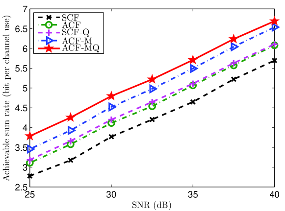
Figure 3: Performance comparison in a two-hop system.

The simulated sum-rate performances are compared in Fig. 3. We see that ACF outperforms SCF by about $2\textrm{ dB}$. Also, SCF-Q outperforms SCF by about $2\textrm{ dB}$, due to the use of asymmetric quantization; ACF-M outperforms ACF by about $2\textrm{ dB}$, due to the use of asymmetric modulo operation; ACF-MQ outperforms ACF by about $3\textrm{ dB}$, due to the use of both asymmetric modulo operation and asymmetric quantization; ACF-MQ outperforms SCF by about $5\textrm{ dB}$, thanks to the use of asymmetric shaping lattices, asymmetric modulo operation, and asymmetric quantization. Fig. 3 demonstrates clearly the the performance advantage of the proposed CCF scheme over the conventional CF scheme.

VIII-C2 Performance Comparison With Different Network Sizes

We now provide the performance comparison with different network sizes. Because of high computation complexity, we only simulate the performance of SCF and SCF-Q schemes. In Fig. 4, we see that, for a $2\times 2$ network (with two sources and two relays), the power gain of SCF-Q over SCF is about $2\textrm{ dB}$ at high SNR; for a $4\times 4$ network, the corresponding power gain is about $6\textrm{ dB}$. We see that the performance gain of SCF-Q increases significantly with the network size.

It is highly desirable to understand how the performance of CCF improves with the network size. This requires the development of more efficient algorithms to solve (53), which is nevertheless an interesting topic for future research.

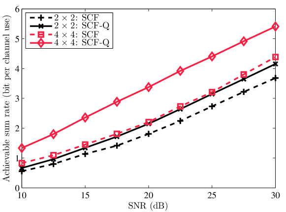
Figure 4: Performance comparison with different network sizes.

IX Conclusions

In this paper, we proposed a novel relay strategy, named CCF, to exploit the asymmetry naturally inherent in wireless networks. Compared with conventional CF, CCF includes an extra compressing stage in between the computing and forwarding stages. We proposed to use quantization and modulo operation for compressing the message combinations computed at relays, which reduces the information redundancy in the messages forwarded by the relays and thereby improve the spectral efficiency of the network. Particularly, we studied CCF design in a two-hop wireless relaying network involving multiple sources, multiple relays, and a single destination. We derived achievable rates of the scheme and formulate a sum-rate maximization problem for performance optimization. Numerical results were presented to demonstrate the significant performance advantage of CCF over CF.

Appendix A Proof of Lemma 1

We follow Algorithm 1 step by step to prove that the output of Algorithm 1 satisfies $\hat{\mathbf{t}}_{l}=\mathbf{t}_{l},l=1,\cdots,L$. Recall that Algorithm 1 involves $L$ iterations. In the $j$-th iteration, $\left\{\hat{\mathbf{t}}_{l,j},l\in\mathcal{S}^{\left\langle j\right\rangle}\right\}$ is computed using $\left\{\mathbf{v}_{m}^{\left\langle j\right\rangle},m\in\mathcal{T}^{\left\langle j\right\rangle}\right\}$, where $\mathbf{v}_{m}^{\left\langle j\right\rangle}$ is set as $\mathbf{v}_{m}$ for $j=1$, and given in (38) for $j>1$.

We first prove that, in the $j$-th iteration,

$$\mathbf{v}_{m}^{\left\langle j\right\rangle}=\left[\sum_{l=1}^{L}a_{ml}\sum_{\mu=j}^{L}\mathbf{t}_{l,\mu}\right]\bmod\Lambda_{s}$$ (57)

for $m\in\mathcal{T}^{\left\langle j\right\rangle}$. We prove this statement by induction. In initialization, we have $\mathbf{v}_{m}^{\left\langle 1\right\rangle}=\mathbf{v}_{m},m\in\mathcal{T}^{\left\langle 1\right\rangle}$. For $j=1$, the residual relay set only contains one element, i.e., $\mathcal{T}^{\left\langle 1\right\rangle}=\left\{\pi_{d}^{-1}\left(1\right)\right\}$, and $\Lambda_{d,\pi_{d}^{-1}\left(1\right)}=\Lambda_{A,1}$ is the finest lattice in $\left\{\Lambda_{c,l}\right\}$. Then

$$\medspace\mathbf{v}_{\pi_{d}^{-1}\left(1\right)}^{\left\langle 1\right\rangle}=\mathbf{v}_{\pi_{d}^{-1}\left(1\right)}$$ (58a)

$$= \medspace\left[\sum_{l=1}^{L}a_{\pi_{d}^{-1}\left(1\right)l}\left(\mathbf{t}_{l}-Q_{\Lambda_{s}}\left(\mathbf{t}_{l}-\mathbf{d}_{l}\right)\right)\right]\bmod\Lambda_{s}$$ (58b)

$$= \medspace\left[\sum_{l=1}^{L}a_{\pi_{d}^{-1}\left(1\right)l}\sum_{\mu=1}^{L}\mathbf{t}_{l,\mu}\right]\bmod\Lambda_{s}$$ (58c)

where (58b) follows from (28) and $\sum_{l=1}^{L}a_{\pi_{d}^{-1}\left(1\right)l}\left(\mathbf{t}_{l}-Q_{\Lambda_{s}}\left(\mathbf{t}_{l}-\mathbf{d}_{l}\right)\right)\in\Lambda_{A,1}$; (58c) follows from (31). Thus (57) holds for $j=1$.

Now suppose that (57) holds for the $j$-th iteration. We show that $\hat{\mathbf{t}}_{l,j}=\mathbf{t}_{l,j},l\in\mathcal{S}^{\langle j\rangle}$ in the $j$-th iteration, and that (57) still holds for the $\left(j+1\right)$-th iteration.

In Line 5, with $\left\{\hat{\mathbf{v}}_{m}^{\left\langle j\right\rangle}\right\}$, we obtain

$$\hat{\mathbf{v}}_{m}^{\left\langle j\right\rangle}\negmedspace\bmod\negmedspace\Lambda_{A,j+1} = \left[\negthinspace\sum_{l=1}^{L}\negthinspace a_{ml}\negthinspace\sum_{\mu=j}^{L}\negthinspace\mathbf{t}_{l,\mu}\negthinspace\right]\negthickspace\bmod\negmedspace\Lambda_{A,j+1}$$ (59a)

$$= \left[\sum_{l=1}^{L}a_{ml}\mathbf{t}_{l,j}\right]\bmod\Lambda_{A,j+1}$$ (59b)

$$= \left[\sum_{l\in\mathcal{S}^{\left\langle j\right\rangle}}\negmedspace a_{ml}\mathbf{t}_{l,j}\right]\negthickspace\bmod\Lambda_{A,j+1}$$ (59c)

for all $m\in\mathcal{T}^{\left\langle j\right\rangle}$, where (59a) holds since (57) is true for the $j$-th iteration; (59b) follows from $\mathbf{t}_{l,\mu}\bmod\Lambda_{A,j+1}=0$, for $\mu>j$, since $\mathbf{t}_{l,\mu}\in\Lambda_{A,\mu}\cap\mathcal{V}_{A,\mu+1}$; (59c) follows from $\mathbf{t}_{l,j}=\mathbf{0}$ for $l\notin\mathcal{S}^{\left\langle j\right\rangle}$ by the definition of $\mathbf{t}_{l,j}$ and $\mathcal{S}^{\left\langle j\right\rangle}$. Also by the definition of $\mathbf{t}_{l,j}$, we have $\mathbf{t}_{l,j}\in\mathcal{C}_{e}^{\left\langle j\right\rangle}=\Lambda_{A,j}\cap\mathcal{V}_{A,j+1}$. In Line 5 of Algorithm 1, $\psi^{-\left\langle j\right\rangle}$ maps $\mathbf{t}_{l,j}$ from $\mathcal{C}_{e}^{\left\langle j\right\rangle}$ to the finite field $\mathbb{F}_{\gamma}^{k}$. Denote $\mathbf{w}_{l,j}=\psi^{-\left\langle j\right\rangle}\left(\mathbf{t}_{l,j}\right)$, for $l=1,\cdots,L$. From (36) and Lemma 6 in [1], we obtain the following isomorphism:

$$\sum_{l\in\mathcal{S}^{\left(i\right)}}q_{ml}\mathbf{w}_{l,j}=\psi^{-\left\langle j\right\rangle}\left(\left[\sum_{l\in\mathcal{S}^{\left\langle j\right\rangle}}a_{ml}\mathbf{t}_{l,j}\right]\bmod\Lambda_{A,j+1}\right).$$ (60)

Then by (59) we have

$$\sum_{l\in\mathcal{S}^{\left(i\right)}}q_{ml}\mathbf{w}_{l,j} = \psi^{-\left\langle j\right\rangle}\left(\hat{\mathbf{v}}_{m}^{\left\langle j\right\rangle}\bmod\Lambda_{A,j+1}\right).$$ (61)

Stacking the two sides of (61) for $m\in\mathcal{T}^{\left\langle j\right\rangle}$ in a row-by-row manner gives a matrix equation over $\mathbb{F}_{\gamma}$:

$$\mathbf{Q}^{\left\langle j\right\rangle}\mathbf{W}^{\left\langle j\right\rangle}=\mathbf{U}^{\left\langle j\right\rangle}$$ (62)

where the rows in $\mathbf{W}^{\left\langle j\right\rangle}$ are specified by $\mathbf{w}_{l,j}^{T},l\in\mathcal{S}^{\left\langle j\right\rangle}$ and $\mathbf{U}^{\left\langle j\right\rangle}$ is the matrix obtained in (38) of Algorithm 1. Recall that $\mathbf{Q}^{\left\langle j\right\rangle}$ is of full rank by assumption. We obtain from (62) that

$$\mathbf{W}^{\left\langle j\right\rangle}=\left(\mathbf{Q}^{\left\langle j\right\rangle}\right)^{-1}\mathbf{U}^{\left\langle j\right\rangle}=\hat{\mathbf{W}}^{\left\langle j\right\rangle}.$$ (63)

Thus, we can obtain $\mathbf{w}_{l,j},l\in\mathcal{S}^{\left\langle j\right\rangle}$ from (63). Then

$$\psi^{\left\langle j\right\rangle}\left(\mathbf{w}_{l,j}\right)=\mathbf{t}_{l,j}=\hat{\mathbf{t}}_{l,j},l\in\mathcal{S}^{\left\langle j\right\rangle}.$$ (64)

Note that $\mathbf{w}_{l,j}^{T}$ is in general not the $l$-th row of $\mathbf{W}^{\left\langle j\right\rangle}$.

Then we cancel the contribution of $\left\{\sum_{\mu=\pi_{c}\left(l\right)}^{j}\mathbf{t}_{l,\mu},l\in\mathcal{S}^{\left\langle j\right\rangle}\right\}$ from $\left\{\mathbf{v}_{m},m\in\mathcal{T}^{\left\langle j+1\right\rangle}\right\}$, yielding (66) for $m\in\mathcal{T}^{\left\langle j+1\right\rangle}$, where (66b) is from (38) and (28); (66c) and (66e) utilizes the fact that, for $\mathbf{x}_{1}\in\mathbb{R}^{n},\mathbf{x}_{2}\in\Lambda$,

$$Q_{\Lambda}\left(\mathbf{x}_{1}+\mathbf{x}_{2}\right) = \mathbf{x}_{1}+\mathbf{x}_{2}-\left(\mathbf{x}_{1}+\mathbf{x}_{2}\right)\bmod\Lambda$$ (65a)

$$= Q_{\Lambda}\left(\mathbf{x}_{1}\right)+\mathbf{x}_{2}$$ (65b)

and (66f) follows by noting

$$Q_{\Lambda_{d,m}}\negmedspace\left(\sum_{l=1}^{L}a_{ml}\sum_{\mu=1}^{j}\mathbf{t}_{l,\mu}\right)=Q_{\Lambda_{d,m}}\left(\sum_{l\in\mathcal{S}^{\left\langle j\right\rangle}}\negmedspace a_{ml}\negmedspace\sum_{\mu=\pi_{c}\left(l\right)}^{j}\mathbf{t}_{l,\mu}\right)$$

by the definition of $\mathcal{S}^{\left\langle j\right\rangle}$ in (34) and $\mathbf{t}_{l,\mu}=0$ for $\mu<\pi_{c}\left(l\right)$. Eq. (66) shows that (57) holds for the $\left(j+1\right)$-th iteration as well. Thus, (57) holds by induction.

$$\mathbf{v}_{m}^{\left\langle j+1\right\rangle}$$ (66a)

$$= \left[Q_{\Lambda_{d,m}}\negthickspace\left(\sum_{l=1}^{L}\negmedspace a_{ml}\negthickspace\left(\negmedspace\sum_{\mu=1}^{L}\mathbf{t}_{l,\mu}\negmedspace-\negmedspace Q_{\Lambda_{s}}\left(\mathbf{t}_{l}-\mathbf{d}_{l}\right)\right)\negthickspace\right)\negmedspace-\negmedspace Q_{\Lambda_{d,m}}\negthickspace\left(\sum_{l\in\mathcal{S}^{\left\langle j\right\rangle}}\negmedspace a_{ml}\negthickspace\sum_{\mu=\pi_{c}\left(l\right)}^{j}\negmedspace\mathbf{t}_{l,\mu}\right)\right]\negthickspace\bmod\Lambda_{s}$$ (66b)

$$= \left[\negmedspace Q_{\Lambda_{d,m}}\negthickspace\left(\sum_{l=1}^{L}\negmedspace a_{ml}\negthickspace\sum_{\mu=1}^{L}\negmedspace\mathbf{t}_{l,\mu}\negmedspace\right)\negmedspace-\negthickspace\sum_{l=1}^{L}\negmedspace a_{ml}Q_{\Lambda_{s}}\negmedspace\left(\mathbf{t}_{l}-\mathbf{d}_{l}\right)\negmedspace-\negmedspace Q_{\Lambda_{d,m}}\negthickspace\left(\negthickspace\sum_{l\in\mathcal{S}^{\left\langle j\right\rangle}}\negthickspace a_{ml}\negthickspace\sum_{\mu=\pi_{c}\left(l\right)}^{j}\negthickspace\mathbf{t}_{l,\mu}\right)\negmedspace\right]\negthickspace\bmod\Lambda_{s}$$ (66c)

$$= \left[Q_{\Lambda_{d,m}}\left(\sum_{l=1}^{L}a_{ml}\sum_{\mu=1}^{L}\mathbf{t}_{l,\mu}\right)-Q_{\Lambda_{d,m}}\left(\sum_{l\in\mathcal{S}^{\left\langle j\right\rangle}}a_{ml}\sum_{\mu=\pi_{c}\left(l\right)}^{j}\mathbf{t}_{l,\mu}\right)\right]\bmod\Lambda_{s}$$ (66d)

$$= \left[Q_{\Lambda_{d,m}}\negmedspace\left(\sum_{l=1}^{L}\negmedspace a_{ml}\negmedspace\sum_{\mu=1}^{j}\negmedspace\mathbf{t}_{l,\mu}\right)\negmedspace+\negmedspace\sum_{l=1}^{L}\negmedspace a_{ml}\negmedspace\sum_{\mu=j+1}^{L}\negmedspace\mathbf{t}_{l,\mu}\negmedspace-\negmedspace Q_{\Lambda_{d,m}}\left(\negmedspace\sum_{l\in\mathcal{S}^{\left\langle j\right\rangle}}\negmedspace a_{ml}\negthickspace\sum_{\mu=\pi_{c}\left(l\right)}^{j}\negmedspace\mathbf{t}_{l,\mu}\right)\right]\negmedspace\bmod\Lambda_{s}$$ (66e)

$$= \left[\sum_{l=1}^{L}a_{ml}\sum_{\mu=j+1}^{L}\mathbf{t}_{l,\mu}\right]\bmod\Lambda_{s}$$ (66f)

Since Algorithm 1 recovers $\left\{\mathbf{t}_{l,j},l\in\mathcal{S}^{\left\langle j\right\rangle}\right\}$ by (64) for $j=1,\cdots,L$, and $\mathbf{t}_{l,j}=\mathbf{0}$ for $l\notin\mathcal{S}^{\left\langle j\right\rangle}$, we see that all $\left\{\mathbf{t}_{l,j}\right\}$ are recovered. Finally, Algorithm 1 recovers $\left\{\mathbf{t}_{l}\right\}$ by (32), which concludes the proof.

Furthermore, from (64) and $\mathbf{t}_{l,j}=\mathbf{0}$ for $l\notin\mathcal{S}^{\left\langle j\right\rangle}$, we see that

$$\hat{\mathbf{t}}_{l}=\left[\sum_{\mu=\pi_{c}\left(j\right)}^{L}\hat{\mathbf{t}}_{l,\mu}\right]\bmod\Lambda_{s}=\left[\sum_{\mu=\pi_{c}\left(l\right)}^{L}\mathbf{t}_{l,\mu}\right]\bmod\Lambda_{s}=\mathbf{t}_{l}$$

which concludes the proof.

Appendix B Proof of Lemma 2

By assumption, $\mathbf{Q}^{\left\langle L\right\rangle}=\mathbf{Q}$ is of full rank. From (34) and (35), we see that $\mathbf{Q}^{\left\langle j-1\right\rangle}$ can be obtained by deleting one row (corresponding to the $\pi_{d}^{-1}\left(j\right)$-th relay) and one column (corresponding to the $\pi_{c}^{-1}\left(j\right)$-th source) from $\mathbf{Q}^{\left\langle j\right\rangle}$.

Suppose $\mathbf{Q}^{\left\langle j\right\rangle}\in\mathbb{F}_{\gamma}^{j\times j},j>1,$ is of full rank, and we want to find a $\mathbf{Q}^{\left\langle j-1\right\rangle}\in\mathbb{F}_{\gamma}^{\left(j-1\right)\times\left(j-1\right)}$ of full rank. Since $\pi_{c}\left(\cdot\right)$ is given, we delete the corresponding column of $\mathbf{Q}^{\left\langle j\right\rangle}$, yielding a matrix $\tilde{\mathbf{Q}}^{\left\langle j\right\rangle}$ of rank $\left(j-1\right)$. From linear algebra, there always exists at least one full-rank $\mathbf{Q}^{\left\langle j-1\right\rangle}$ obtained by deleting one row of $\tilde{\mathbf{Q}}^{\left\langle j\right\rangle}$. Choose such a $\mathbf{Q}^{\left\langle j-1\right\rangle}$ (with rank $\left(j-1\right)$) and set the corresponding value of $\pi_{d}\left(\cdot\right)$ according to the index of the deleted row. By induction, we obtain full-rank $\mathbf{Q}^{\left\langle L\right\rangle},\cdots,$ and $\mathbf{Q}^{\left\langle 1\right\rangle}$.

Appendix C Proof of Lemma 3

We follow Algorithm 2 step by step to prove that the output of Algorithm 2 satisfies $\hat{\mathbf{t}}_{l}=\mathbf{t}_{l},l=1,\cdots,L$. Algorithm 2 involves $L$ iterations. In the $i$-th iteration, $\mathbf{t}_{\pi_{s}^{-1}\left(i\right)}$ is recovered with $\left\{\mathbf{v}_{m}^{\left(i\right)},m\in\mathcal{T}^{\left(i\right)}\right\}$, where $\mathbf{v}_{m}^{\left(i\right)}$ is the lattice equation from the $m$-th relay at the $i$-th iteration.

We first prove that, in the $i$-th iteration,

$$\mathbf{v}_{m}^{\left(i\right)}=\left[\sum_{l\in\mathcal{S}^{\left(i\right)}}a_{ml}\left(\mathbf{t}_{l}-Q_{\Lambda_{s,l}}\left(\mathbf{t}_{l}-\mathbf{d}_{l}\right)\right)\right]\bmod\Lambda_{e,m}$$ (67)

for $m\in\mathcal{T}^{\left(i\right)}$, and that exactly one of $\left\{\mathbf{t}_{l}\right\}$ is restored in each iteration. We prove this statement by induction. The algorithm sets $\mathbf{v}_{m}^{\left(1\right)}=\mathbf{v}_{m},m\in\mathcal{T}^{\left(1\right)}$, at the initialization stage. We immediately see that (67) holds for $i=1$. Now suppose that (67) holds for the $i$-th iteration. We will show that $\mathbf{t}_{\pi_{s}^{-1}\left(i\right)}$ is recovered in the $i$-th iteration, and that (67) also holds for the $\left(i+1\right)$-th iteration.

By the definition of $\mathcal{S}^{\left(i\right)}$ and $\mathcal{T}^{\left(i\right)}$, $\Lambda_{B,i}=\Lambda_{s,\pi_{s}^{-1}\left(i\right)}$ is the finest in $\left\{\Lambda_{s,l}|l\in\mathcal{S}^{\left(i\right)}\right\}$, and also the finest in $\left\{\Lambda_{e,m}|m\in\mathcal{T}^{\left(i\right)}\right\}$. Then, with $\left\{\mathbf{v}_{m}^{\left(i\right)}\right\}$, we obtain

$$\mathbf{v}_{m}^{\left(i\right)}\bmod\Lambda_{B,i}$$ (68)

$$= \left[\sum_{l\in\mathcal{S}^{\left(i\right)}}a_{ml}\left(\mathbf{t}_{l}-Q_{\Lambda_{s,l}}\left(\mathbf{t}_{l}-\mathbf{d}_{l}\right)\right)\right]\bmod\Lambda_{B,i}$$

$$= \left[\sum_{l\in\mathcal{S}^{\left(i\right)}}a_{ml}\left(\mathbf{t}_{l}\bmod\Lambda_{B,i}\right)\right]\bmod\Lambda_{B,i}$$

where $\mathbf{t}_{l}\bmod\Lambda_{B,i}$ is a codeword in the effective lattice codebook $\mathcal{C}_{e}^{\left(i\right)}$ defined in Subsection VI-C. That is, $\mathbf{t}_{l}\bmod\Lambda_{B,i}$ can be seen as from a common codebook $\mathcal{C}_{e}^{\left(i\right)}$. Note that

$$\mathbf{t}_{\pi_{s}^{-1}\left(i\right)}\bmod\Lambda_{B,i}=\mathbf{t}_{\pi_{s}^{-1}\left(i\right)}$$ (69)

since $\Lambda_{B,i}=\Lambda_{s,\pi_{s}^{-1}\left(i\right)}$.

Define $\mathbf{w}_{l}^{\left(i\right)}=\psi^{-\left(i\right)}\left(\mathbf{t}_{l}\bmod\Lambda_{B,i}\right)$, for $l=1,\cdots,L$. By (68), (46), and Lemma 6 in [1], we have

$$\sum_{l\in\mathcal{S}^{\left(i\right)}}q_{ml}\mathbf{w}_{l}^{\left(i\right)}=\psi^{-\left(i\right)}\left(\mathbf{v}_{m}^{\left(i\right)}\bmod\Lambda_{B,i}\right).$$ (70)

Form the matrix $\mathbf{W}^{\left(i\right)}$ by stacking $\mathbf{w}_{l}^{\left(i\right)T},l\in\mathcal{S}^{\left(i\right)}$, row by row. Similarly, form the matrix $\mathbf{U}^{\left(i\right)}$ by stacking $\left(\psi^{-\left(i\right)}\left(\mathbf{v}_{m}^{\left(i\right)}\bmod\Lambda_{B,i}\right)\right)^{T},m\in\mathcal{T}^{\left(i\right)}$. We can write (70) as

$$\mathbf{Q}^{\left(i\right)}\mathbf{W}^{\left(i\right)}=\mathbf{U}^{\left(i\right)},$$ (71)

which is a matrix equation over $\mathbb{F}_{\gamma}^{k}$. Then

$$\mathbf{W}^{\left(i\right)}=\left(\mathbf{Q}^{\left(i\right)}\right)^{-1}\mathbf{U}^{\left(i\right)}=\hat{\mathbf{W}}^{\left(i\right)}$$ (72)

where $\mathbf{Q}^{\left(i\right)}$ is of full rank by assumption. From (69), we have $\mathbf{w}_{\pi_{s}^{-1}\left(i\right)}=\mathbf{w}_{\pi_{s}^{-1}\left(i\right)}^{\left(i\right)}$. By setting $\hat{\mathbf{w}}_{\pi_{s}^{-1}\left(i\right)}^{T}$ as the corresponding row of $\hat{\mathbf{W}}^{\left(i\right)}$ in Line 6, we recover the message as $\hat{\mathbf{w}}_{\pi_{s}^{-1}\left(i\right)}=\mathbf{w}_{\pi_{s}^{-1}\left(i\right)}$, and the lattice codeword as

$$\hat{\mathbf{t}}_{\pi_{s}^{-1}\left(i\right)}=\mathbf{t}_{\pi_{s}^{-1}\left(i\right)}.$$

That is, the lattice codeword of the $\pi_{s}^{-1}\left(i\right)$-th source is correctly recovered.

Then the destination cancels the contribution of $\mathbf{t}_{\pi_{s}^{-1}\left(i\right)}$ and $\mathbf{d}_{\pi_{s}^{-1}\left(i\right)}$ from $\mathbf{v}_{m}^{\left(i\right)}$ in Line 7 of Algorithm 2 to obtain $\mathbf{v}_{m}^{\left(i+1\right)}$. By noting $\mathcal{S}^{\left(i+1\right)}=\mathcal{S}^{\left(i\right)}\setminus\left\{\pi_{s}^{-1}\left(i\right)\right\}$ and $\mathcal{T}^{\left(i+1\right)}=\mathcal{T}^{\left(i\right)}\setminus\left\{\pi_{e}^{-1}\left(i\right)\right\}$, we have

$$\mathbf{v}_{m}^{\left(i+1\right)}\negmedspace=\negmedspace\left[\negmedspace\sum_{l\in\mathcal{S}^{\left(i+1\right)}}\negthickspace a_{ml}\left(\mathbf{t}_{l}-Q_{\Lambda_{s,l}}\left(\mathbf{t}_{l}-\mathbf{d}_{l}\right)\right)\right]\negthickspace\bmod\negmedspace\Lambda_{e,m}$$ (73)

for $m\in\mathcal{T}^{\left(i+1\right)}$, which establishes (67) by induction. This concludes the proof of Theorem 3.

Appendix D Proof of Lemma 4

By assumption, $\mathbf{Q}^{\left(1\right)}=\mathbf{Q}$ is of full rank. From (44) and (45), we see that $\mathbf{Q}^{\left(i+1\right)}$ can be obtained by deleting one row (corresponding to the $\pi_{e}^{-1}\left(j\right)$-th relay) and one column (corresponding to the $\pi_{s}^{-1}\left(j\right)$-th source) from $\mathbf{Q}^{\left(i\right)}$.

Suppose $\mathbf{Q}^{\left(i\right)}\in\mathbb{F}_{\gamma}^{\left(L-i+1\right)\times\left(L-i+1\right)},i>1,$ is of full rank, and we want to find a $\mathbf{Q}^{\left(i+1\right)}\in\mathbb{F}_{\gamma}^{\left(L-i\right)\times\left(L-i\right)}$ of full rank. Since $\pi_{s}\left(\cdot\right)$ is given, we delete the corresponding column of $\mathbf{Q}^{\left(i\right)}$, yielding a matrix $\tilde{\mathbf{Q}}^{\left(i\right)}$ of rank $\left(L-i\right)$. From linear algebra, there always exists at least one full-rank $\mathbf{Q}^{\left(i+1\right)}$ obtained by deleting one row of $\tilde{\mathbf{Q}}^{\left(i\right)}$. Choose such a $\mathbf{Q}^{\left(i+1\right)}$ (with rank $\left(L-i\right)$) and set the corresponding value of $\pi_{e}\left(\cdot\right)$ according to the index of the deleted row. By induction, we can obtain $\mathbf{Q}^{\left(1\right)},\cdots,\mathbf{Q}^{\left(L\right)}$ that are all of full rank.

Appendix E Proof of Lemma 5

In Section VII, we have shown that the SRQ algorithm can be applied on $\left\{\mathbf{v}_{m}\bmod\Lambda_{B,1}\right\}$ to recover $\left\{\mathbf{t}_{l}\bmod\Lambda_{B,1}\right\}$. We next show that the SRM algorithm can be used to recover $\left\{Q_{\Lambda_{B,1}}\left(\mathbf{t}_{l}\right)\right\}$. From Line 3 of the SRMQ algorithm, we have

$$\hat{\mathbf{t}}_{l}^{\textrm{quan}} = \left[\sum_{\mu=1}^{L}\mathbf{t}_{l,\mu}\right]\bmod\Lambda_{B,1}$$ (74a)

$$= \left[\sum_{\mu=1}^{L}\mathbf{t}_{l,\mu}+\mathbf{t}_{l,L+1}\right]\bmod\Lambda_{B,1}$$ (74b)

$$= \mathbf{t}_{l}\bmod\Lambda_{B,1}$$ (74c)

where step (74b) follows from $\mathbf{t}_{l,L+1}\in\Lambda_{B,1}$, step (74c) from (50). In Line 4, we cancel $\left\{\hat{\mathbf{t}}_{l}^{\textrm{quan}}\right\}$ from $\left\{\mathbf{v}_{m}\right\}$, yielding

$$\mathbf{v}_{m}^{\textrm{quan}}$$ (75a)

$$= \left[\mathbf{v}_{m}-Q_{\Lambda_{d,m}}\left(\sum_{l=1}^{L}a_{ml}\hat{\mathbf{t}}_{l}^{\textrm{quan}}\right)\right]\bmod\Lambda_{e,m}$$ (75b)

$$= \left[\sum_{l=1}^{L}a_{ml}\left(\mathbf{t}_{l}-\hat{\mathbf{t}}_{l}^{\textrm{quan}}-Q_{\Lambda_{s,l}}\left(\mathbf{t}_{l}-\mathbf{d}_{l}\right)\right)\right]\bmod\Lambda_{e,m}$$ (75c)

$$= \left[\negmedspace\sum_{l=1}^{L}\negmedspace a_{ml}\negmedspace\left(Q_{\negthinspace\Lambda_{\negthinspace B\negthinspace,1}}\negthickspace\left(\mathbf{t}_{l}\right)\negmedspace-\negmedspace Q_{\negthinspace\Lambda_{\negthinspace s\negthinspace,l}}\negthickspace\left(\negthinspace Q_{\negthinspace\Lambda_{\negthinspace B\negthinspace,1}}\negthickspace\left(\mathbf{t}_{l}\right)\negmedspace-\negmedspace\left(\negthinspace\mathbf{d}_{l}\negmedspace-\negmedspace\hat{\mathbf{t}}_{l}^{\textrm{quan}}\negthinspace\right)\right)\right)\negmedspace\right]\negthickspace\bmod\negthickspace\Lambda_{\negthinspace e\negthinspace,m}$$ (75d)

where (75c) follows from (48) and (65), (75d) from the fact of $\hat{\mathbf{t}}_{l}^{\textrm{quan}}=\mathbf{t}_{l}\bmod\Lambda_{B,1}$. Note that $\mathbf{v}_{m}^{\textrm{quan}}$ in (75d) is actually a special case of (39) with $\mathbf{t}_{l}$ replaced by $Q_{\Lambda_{B,1}}\left(\mathbf{t}_{l}\right)$, and $\mathbf{d}_{l}$ replaced by $\mathbf{d}_{l}^{\textrm{quan}}=\mathbf{d}_{l}-\hat{\mathbf{t}}_{l}^{\textrm{quan}}$, for $l=1,\cdots,L$. Therefore, we can apply the SRM algorithm to $\left\{\mathbf{v}_{m}^{\textrm{quan}}\right\}$, yielding outputs $\left\{\hat{\mathbf{t}}_{l}^{\textrm{mod}}=Q_{\Lambda_{B,1}}\left(\mathbf{t}_{l}\right)\right\}$. Finally, we obtain

$$\hat{\mathbf{t}}_{l}=\hat{\mathbf{t}}_{l}^{\textrm{quan}}+\hat{\mathbf{t}}_{l}^{\textrm{mod}}=\mathbf{t}_{l}\bmod\Lambda_{B,1}+Q_{\Lambda_{B,1}}\left(\mathbf{t}_{l}\right)=\mathbf{t}_{l}$$ (76)

for $$l=1,\cdots,L$$,

which follows from (3) and (74).

References

• [1] B. Nazer and M. Gastpar, “Compute-and-forward: Harnessing interference through structured codes,” IEEE Trans. Inf. Theory, vol. 57, no. 10, pp. 6463–6486, 2011.
• [2] U. Niesen and P. Whiting, “The degrees of freedom of compute-and-forward,” IEEE Trans. Inf. Theory, vol. 58, no. 8, pp. 5214–5232, 2012.
• [3] A. Osmane and J.-C. Belfiore, “The compute-and-forward protocol: implementation and practical aspects,” arXiv:1107.0300, 2011.
• [4] V. Ntranos, V. R. Cadambe, B. Nazer, and G. Caire, “Asymmetric compute-and-forward,” in 2013 51st Annual Allerton Conference on Communication, Control, and Computing (Allerton), Oct. 2-4 2013, pp. 1174–1181.
• [5] J. Zhu and M. Gastpar, “Asymmetric compute-and-forward with CSIT,” arXiv:1401.3189, 2014.
• [6] Z. Fang, X. Yuan, and X. Wang, “Towards the asymptotic sum capacity of the MIMO cellular two-way relay channel,” IEEE Trans. Signal Process., vol. 62, no. 16, pp. 4039–4051, Aug. 2014.
• [7] X. Yuan, “MIMO multiway relaying with clustered full data exchange: Signal space alignment and degrees of freedom,” Trans. Wireless Commun., vol. 13, no. 12, pp. 6795–6808, Dec. 2014.
• [8] X. Yuan, T. Yang, and I. Collings, “Multiple-input multiple-output two-way relaying: A space-division approach,” IEEE Trans. Inf. Theory, vol. 59, no. 10, pp. 6421–6440, Oct. 2013.
• [9] F. Wang, X. Yuan, S. C. Liew, and D. Guo, “Wireless MIMO switching: Weighted sum mean square error and sum rate optimization,” IEEE Trans. Inf. Theory, vol. 59, no. 9, pp. 5297–5312, Sept. 2013.
• [10] R. Wang and X. Yuan, “MIMO multiway relaying with pair-wise data exchange: A degrees of freedom perspective,” IEEE Trans. Signal Process., vol. 62, no. 20, pp. 5294–5307, Oct. 2014.
• [11] Y. Tan, X. Yuan, S. C. Liew, and A. Kavcic, “Asymmetric compute-and-forward: Going beyond one hop,” in Proc. 52nd Annual Allerton Conference on Communication, Control, and Computing, Allerton, USA, Oct. 1-3 2014, pp. 667–674.
• [12] B. Hern and K. Narayanan, “Multilevel coding schemes for compute-and-forward with flexible decoding,” IEEE Trans. Inf. Theory, vol. 59, no. 11, pp. 7613–7631, Nov. 2013.
• [13] T. Huang, J. Yuan, and Q. Sun, “Opportunistic pair-wise compute-and-forward in multi-way relay channels,” in Proc. IEEE Int. Conf. Commun. (ICC), June 2013, pp. 4614–4619.
• [14] Y.-C. Huang, N. E. Tunali, and K. R. Narayanan, “A compute-and-forward scheme for gaussian bi-directional relaying with inter-symbol interference,” IEEE Trans. Commun., vol. 61, no. 3, pp. 1011–1019, 2013.
• [15] H. J. Yang, Y. Choi, N. Lee, and A. Paulraj, “Achievable sum-rate of MU-MIMO cellular two-way relay channels: Lattice code-aided linear precoding,” IEEE J. Sel. Areas Commun., vol. 30, no. 8, pp. 1304–1318, 2012.
• [16] D. Gunduz, A. Yener, A. Goldsmith, and H. V. Poor, “The multiway relay channel,” IEEE Trans. Inf. Theory, vol. 59, no. 1, pp. 51–63, 2013.
• [17] K. Lee, N. Lee, and I. Lee, “Achievable degrees of freedom on k-user y channels,” IEEE Trans. Wireless Commun., vol. 11, no. 3, pp. 1210–1219, 2012.
• [18] Y. Tian and A. Yener, “Degrees of freedom for the MIMO multi-way relay channel,” in Proc. IEEE ISIT, 2013, pp. 1576–1580.
• [19] W. Nam, S.-Y. Chung, and Y. H. Lee, “Nested lattice codes for gaussian relay networks with interference,” IEEE Trans. Inf. Theory, vol. 57, no. 12, pp. 7733–7745, 2011.
• [20] O. Ordentlich and U. Erez, “A simple proof for the existence of “good” pairs of nested lattices,” in Proceedings of the 27th Convention of Electrical & Electronics Engineers in Israel (IEEEI), 2012, pp. 1–12.
• [21] U. Erez and R. Zamir, “Achieving 1/2log(1+SNR) on the AWGN channel with lattice encoding and decoding,” IEEE Trans. Inf. Theory, vol. 50, no. 10, pp. 2293–2314, Oct. 2004.
• [22] J. H. Conway and N. J. A. Sloane, Sphere packings, lattices and groups.   Springer, 1999, vol. 290.
• [23] C. Feng, D. Silva, and F. R. Kschischang, “An algebraic approach to physical-layer network coding,” IEEE Trans. Inf. Theory, vol. 59, no. 11, pp. 7576–7596, Nov. 2013.
• [24] A. Sakzad, J. Harshan, and E. Viterbo, “Integer-forcing MIMO linear receivers based on lattice reduction,” IEEE Trans. Wireless Commun., vol. 12, no. 10, pp. 4905–4915, 2013.
• [25] W. Nam, S.-Y. Chung, and Y. H. Lee, “Capacity of the Gaussian two-way relay channel to within 1/2 bit,” IEEE Trans. Inf. Theory, vol. 56, no. 11, pp. 5488–5494, 2010.