Quantum Field Theoretic Treatment of Pion Production via Proton Synchrotron Radiation in Strong Magnetic Fields: Effects of Landau Levels

Abstract

We study pion production from proton synchrotron radiation in the presence of strong magnetic fields. We derive the exact proton propagator from the Dirac equation in a strong magnetic field by explicitly including the anomalous magnetic moment. In this exact quantum-field approach the magnitude of pion synchrotron emission turns out to be much smaller than that obtained in the semi-classical approach. However, we also find that the anomalous magnetic moment of the proton greatly enhances the production rate about by two order magnitude.

I Introduction

Magnetic fields in neutron stars play an important role in the interpretation of many observed phenomena. Indeed, strongly magnetized neutron stars (dubbed magnetars pac92 ; mag3 ) hold the key to understanding the asymmetry in supernova (SN) remnants and the still unresolved mechanism for non-spherical SN explosions. Such strong magnetic fields are also closely related to the unknown origin of the kick velocity rothchild94 that proto-neutron stars (PNSs) receive at birth.

It is widely accepted that soft gamma repeaters (SGRs) and anomalous X-ray pulsars (AXPs) correspond to magnetars Mereghetti08 , and that the associate strong magnetic fields have a significant role in production high energy photons. Furthermore, short duration gamma-ray bursts (GRBs) may arise from highly magnetized neutron stars Soderberg06 or mergers of binary neutron stars Gehrels05 ; Bloom026 ; Tanvit13 , and the most popular theoretical models for the long-duration GRBs MacFadyen99 ; MacFadyen01 ; Harikae09 ; Harikae10 invoke magnetized accretion disks around neutron stars or rotating black holes (collapsars) for their central engines. Such magnetars (or black holes with strong magnetic fields) have also been proposed Hillas84 ; Aarons03 as an acceleration site for ultra high-energy (UHE) cosmic rays (UHECRs) and a possible association between magnetar flares Ioka05 and UHECRs has also been observed.

When a particle is accelerated in an external field or in collision with another particle, it can emit quanta corresponding to the field with which the particle interacts. Synchrotron radiation can be produced by high-energy protons accelerated in an environment containing a strong magnetic field. This process has been proposed as a source for high-energy photons in the GeV $-$ TeV range Gupta07 ; Boettcher98 ; Totani98 ; Fragile04 ; Asano07 ; Asano09 , possibly in association with GRBs. Synchrotron emission, however, can occur through any quanta that may couple to an accelerated particle. Since protons strongly couple to meson fields, a high-energy proton can also radiate pions and other mesons, as well as photons.

In fact, the meson-nucleon couplings are about 100 times larger than the photon-nucleon coupling, and the meson production process is expected to exceed photon synchrotron emission in the high energy regime. For example, Refs. Ginzburg65a ; Ginzburg65b ; Zharkov65 ; TK99 ; BDK95 addressed the possibility of $\pi^{0}$ emission from a proton in a strong magnetic field. However, these calculations were performed approximately; i.e. in a semi-classical way and an approximate quantum-mechanical treatment of the proton transitions among the Landau levels of the strong magnetic field.

In the semi-classical approach for the production of synchrotron radiation, the magnetic field strength is characterized by the curvature parameter, $\chi=E_{i}^{2}/(m^{3}R_{c})$, given in terms of the incident particle mass $m$, its energy $E_{i}$, and the curvature radius $R_{c}$. For $\chi<<1~{}(R_{c}>>1)$, the radiation can be treated in a classical way. For example, in a gravitation field or a relatively small electro-magnetic field, charged particles may have such large curvature radii. However, for $\chi>>1~{}(R_{c}<<1)$ i.e., very high energetic particles propagating in the very small curvature radius of a strong magnetic field, quantum effects must be taken into account. Since we consider a proton propagating in a strong magnetic field, which may imply a small Lamor radius $R_{L}=E/(eB)$, the radiation should be also treated in a quantum mechanical way along with the Landau quantization by the magnetic field.

For proton propagation in a strong magnetic field, the value of $\chi$ can be given as

$$\chi={E_{i}^{2}\over{M_{p}^{3}R_{L}}}={{eE_{i}B}\over{M_{p}^{3}}}={E_{i}\over M_{p}}({B_{\perp}\over B_{cr}})~{},$$ (1)

where $B_{cr}=M_{p}^{2}/e$ and $B_{\perp}$ is the magnetic field perpendicular to the proton momentum direction. For illustration, we assume a 1 $\sim$ 5 GeV proton propagating in a strong magnetic field with $B\sim 10^{18}$G, for which $\chi\sim 0.01$. Through analysis of the pion emission based on a quantum field theory treatment, we show that the pion emission can be comparable to the photon emission. In particular, we demonstrate that the anomalous magnetic moment of the charged particle plays a vital roles in the pion synchrotron emission.

In this work, we exploit the Green’s function method for the propagation of protons in a strong magnetic field. This approach has not previously been applied to derive pion synchrotron emission. For the pion-nucleon coupling, the $p$-wave interaction is dominant, and the pion emission amplitude is mainly proportional to $<\mbox{$\overline{\psi}$}_{N}\mbox{$\bm{\sigma}$}\cdot\mbox{$\bm{q}$}\psi_{N}>$, with ${\bm{q}}$ being the emitted pion momentum . Because the pion emission along the direction of the magnetic field is not allowed by the conservation of energy-momentum, $<\mbox{$\overline{\psi}$}_{N}\sigma_{\pm}\psi_{N}>$ has a dominant contribution. Hence, the spin-flip contributions necessary for pseudo-scalar emission are significant.

Section 2 is devoted to an introduction of our theoretical formalism based upon the Green’s function method. Numerical results are presented in section 3 along with detailed discussions. A summary and conclusions are presented in section 4.

II Formalism

II.1 Proton Green’s Function

We assume a uniform magnetic field along the $z$-direction as $\mbox{$\bm{B}$}=(0,0,B)$ and take the electro-magnetic vector potential $A^{\mu}$ to be $A=(0,0,xB,0)$ at the position $\mbox{$\bm{r}$}\equiv(x,y,z)$ .

The relativistic proton wave function ${\tilde{\psi}}$ is obtained from the following Dirac equation:

$$\left[\gamma_{\mu}\cdot(i\partial^{\mu}-eA^{\mu})-m_{N}-\frac{e\kappa_{p}}{2m_{N}}\sigma_{\mu\nu}(\partial^{\mu}A_{\nu}-\partial^{\nu}A^{\mu})\right]\mbox{${\tilde{\psi}}$}(x)=0,$$ (2)

where $m_{N}$ is the proton mass, $\kappa_{p}$ is the proton anomalous magnetic moment (AMM), and $e$ is the elementary charge.

Here, we scale all variables with $\sqrt{eB}$ as $X_{\mu}=\sqrt{eB}x_{\mu}$ and $M_{N}=m_{N}/\sqrt{eB}$, and we write the wave function, e.g.

$$\psi(X)=\left(\begin{array}[]{c}\lambda_{1}f_{n+1}(X-P_{y})\\ \lambda_{2}~{}f_{n}(X-P_{y}){}\\ \lambda_{3}f_{n+1}(X-P_{y})\\ \lambda_{4}~{}f_{n}(X-P_{y}){}\end{array}\right)e^{i(P_{y}X_{2}+P_{z}X_{3}-iEX_{0})}.$$ (3)

Eq. (2) then leads the following characteristic equation:

$$\left[E\gamma_{0}+\sqrt{2(n+1)}\gamma^{2}-P_{z}\gamma^{3}-(\kappa_{p}/M_{N})\Sigma_{z}-M_{N}\right]\mbox{$\bm{\lambda}$}=0$$ (4)

with $\mbox{$\bm{\lambda}$}=(\lambda_{1},\lambda_{2},\lambda_{3},\lambda_{4})$ and $\Sigma_{z}=diag(1,-1,1,-1)$.

Here, the Landau level $n$ starts from $n=-1$ when $s=1$ and from $n=0$ when $s=-1$. We then redefine the Landau number $n_{L}$ as $n_{L}=n+(1+s)/2$. By solving Eq. (4), we then obtain the energy eigenvalues as

$$E(n_{L},P_{z},s)=\pm\sqrt{P_{z}^{2}+(\sqrt{2n_{L}+1-s+M_{N}^{2}}-s\kappa_{p}/M_{N})^{2}}.$$ (5)

The proton Green’s Function $G$ in a magnetic field is written as

$$G = \sum_{n_{L}=0}\sum_{s=\pm 1}\mbox{${\tilde{F}}$}(X)\left[\frac{\rho_{M}^{(+)}(n_{L},s,P_{z})}{P_{0}-E(n_{L},s,P_{z})+i\delta}+\frac{\rho_{M}^{(-)}(n_{L}.x.P_{z})}{P_{0}+E(n_{L},s,P_{z})+i\delta}\right]\mbox{${\tilde{F}}$}(X^{\prime})$$ (6)

with

$${\tilde{F}} = f_{n_{L}+\frac{1-s}{2}}(X-P_{y})\frac{1+\Sigma_{z}}{2}+f_{n_{L}-\frac{1+s}{2}}(X-P_{y})\frac{1-\Sigma_{z}}{2},$$ (7)

$$\rho_{M}^{(+)} = \frac{1}{4E}\left[E\gamma_{0}+\sqrt{2n_{L}+1-s}\gamma^{2}-P_{z}\gamma^{3}+M_{N}+(\kappa_{p}/M_{N})\Sigma_{z}\right]$$ (10)

$$\quad\times\left(1+\frac{s\kappa_{p}/M_{N}}{\sqrt{2n_{L}+1-s+M_{N}^{2}}}+\gamma_{5}\ooalign{\hfil/\hfil\crcr{$a$}}\right),$$

$$\rho_{M}^{(-)} = \frac{1}{4E}\left[E\gamma_{0}-\sqrt{2n_{L}+1-s}\gamma^{2}+P_{z}\gamma^{3}-M_{N}-(\kappa_{p}/M_{N})\Sigma_{z}\right]$$ (13)

$$\quad\times\left(1+\frac{s\kappa_{p}/M_{N}}{\sqrt{2n_{L}+1-s+M_{N}^{2}}}-\gamma_{5}\ooalign{\hfil/\hfil\crcr{$a$}}\right),$$

where $E_{F}$ is the Fermi energy, and the spin vector $a$ is defined as

$$a(p,s)=\left(\frac{sP_{z}}{\sqrt{2n_{L}+1-s+M_{N}^{2}}},0,0,\frac{sE}{\sqrt{2n_{L}+1-s+M_{N}^{2}}}\right).$$ (14)

II.2 Pion Production

In this subsection we consider the pion production rate in the presence of a strong magnetic field. We start the calculation from the following pseudo-vector coupling interaction Lagrangian density as

$${\cal L}=\frac{if_{\pi}}{m_{\pi}}\psi\gamma_{5}\gamma_{\mu}\tau_{a}\psi\partial^{\mu}\phi_{a},$$ (15)

where $f_{\pi}$ is the pseudo-vector pion-nucleon coupling constant, $m_{\pi}$ is the pion mass, and $\phi$ is the pion field. We then calculate the pion decay rate from an initial proton with $n_{L}=n_{i}$, $s=s_{i}$ and $P_{z}=P_{iz}$ to a final proton with $n_{L}=n_{f}$, $s=s_{f}$ and $P_{z}=P_{fz}$. The pion momentum scaled by $\sqrt{eB}$ is written as $Q=(E_{\pi},0,Q_{T},Q_{z})$, where without loss of generality the transverse pion momentum is assumed to be directed along the $y$-axis.

Using the proton propagator, the proton self-energy from one-pion exchange can be written as

$$\Sigma_{\pi}(R_{1},R_{2})=i\left(\frac{f_{\pi}}{M_{\pi}}\right)^{2}\gamma_{\mu}\gamma_{5}\tau_{a}G(R_{1},R_{2})\tau_{a}\gamma_{\nu}\gamma_{5}\partial^{\mu}\partial^{\nu}\Delta_{\pi}(R_{1}-R_{2}),$$

and the decay width is calculated from the imaginary part of the expectation value of the self-energy as

$$\Gamma_{\pi}=-{\rm Im}\int d^{3}R_{1}d^{4}R_{2}\mbox{$\overline{\psi}$}_{i}(R_{1})\Sigma_{\pi}(R_{1},R_{2})\psi_{i}(R_{2}),$$ (16)

where $\Delta_{\pi}$ is the pion propagator.

By performing a Fourier transformation, we can obtain the differential decay width of the proton as

$$\frac{d^{3}\Gamma_{p\pi}/\sqrt{eB}}{dQ^{3}}=\frac{1}{8\pi^{2}E_{\pi}}\left(\frac{f_{\pi}}{M_{\pi}}\right)^{2}\sum_{n_{f},s_{f}}\frac{\delta(E_{f}+E_{\pi}-E_{i})}{4E_{i}E_{f}}W_{if},$$ (17)

with

$$W_{if}=4E_{i}E_{f}{\rm Tr}\left\{\rho_{M}^{(+)}(n_{i},s_{i},P_{z}){\cal O}_{\pi}\rho_{M}^{(+)}(n_{f},s_{f},P_{z}-Q_{z}){\cal O}_{\pi}^{\dagger}\right\},$$ (18)

where $M_{\pi}=m_{\pi}/\sqrt{eB}$, and

$${\cal O}_{\pi} = \int dX\mbox{${\tilde{F}}$}(n_{i},s_{i},X+Q_{T}/2)\gamma_{5}\ooalign{\hfil/\hfil\crcr{Q}}\mbox{${\tilde{F}}$}(n_{f},s_{f},X-Q_{T}/2)$$ (22)

$$= \gamma_{5}\left\{\left[{\cal M}\left(n_{i}+\frac{1-s_{i}}{2},n_{f}+\frac{1-s_{f}}{2}\right)\frac{1+\Sigma_{z}}{2}\right.\right.$$

$$\left.\quad\quad\quad+{\cal M}\left(n_{i}-\frac{1+s_{i}}{2},n_{f}-\frac{1+s_{f}}{2}\right)\frac{1-\Sigma_{z}}{2}\right]\left[\gamma_{0}Q_{0}-\gamma^{3}Q_{z}\right]$$

$$\quad-\left[{\cal M}\left(n_{i}+\frac{1-s_{1}}{2},n_{f}-\frac{1+s_{f}}{2}\right)\frac{1+\Sigma_{z}}{2}\right.$$

$$\left.\left.\quad\quad\quad+{\cal M}\left(n_{i}-\frac{1+s_{i}}{2},n_{f}+\frac{1-s_{f}}{2}\right)\frac{1-\Sigma_{z}}{2}\right]\gamma^{2}Q_{y}\right\}.$$

In the above equation, ${\cal M}(n_{1},n_{2})$ is defined as

$${\cal M}(n_{1},n_{2}) = \int dxf_{n_{1}}\left(x+\frac{Q_{y}}{2}\right)f_{n_{2}}\left(x-\frac{Q_{y}}{2}\right)$$ (23)

$$= (2^{n_{1}+n_{2}}\pi n_{1}!n_{2}!)^{-1/2}e^{-Q_{T}^{2}/4}\int dxe^{-x^{2}}H_{n_{1}}\left(x+\frac{Q_{T}}{2}\right)H_{n_{2}}\left(x-\frac{Q_{T}}{2}\right)$$

$$= \sqrt{\frac{n_{1}!}{n_{2}!}}\left(-\frac{Q_{T}}{\sqrt{2}}\right)^{n_{2}-n_{1}}e^{-\frac{Q_{T}^{2}}{4}}L^{n_{2}-n_{1}}_{n_{1}}\left(\frac{Q_{T}^{2}}{2}\right)\quad\quad(n_{1}\leq n_{2}),$$

$$= \sqrt{\frac{n_{2}!}{n_{1}!}}~{}\left(\frac{Q_{T}}{\sqrt{2}}\right)^{n_{1}-n_{2}}~{}e^{-\frac{Q_{T}^{2}}{4}}L^{n_{1}-n_{2}}_{n_{2}}\left(\frac{Q_{T}^{2}}{2}\right)\quad\quad~{}(n_{1}\geq n_{2}),$$

where $H_{n}(x)$ is the $n$-th Hermite polynomial, and $L_{n}^{m}(x)$ is the associated Laguerre polynomial.

III Results

In this section we show numerical results for pion emission from $1-2$ GeV protons. In the numerical calculation we take the maximum Landau level to be $\sim 3\times 10^{3}$, which somewhat limits our calculations. However, in order to test our model, we choose a proton energy of 1 GeV and a strength of the magnetic field to be $5\times 10^{18}$G. In this case the maximum Landau numbers are $n_{max}=45$ for spin $s=-1$ and $n_{max}=50$ for $s=+1$. Pion production has been shown TK99 to exceed photon emission in the region, $\chi=eBe_{i}/m_{N}^{3}=0.01\sim 1$, in the semi-classical calculation. The value of $\chi$, 0.069, adopted in this calculation belongs in this region.

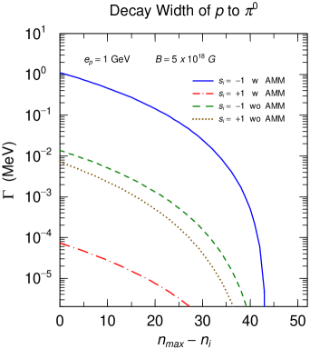
Figure 1: (Color online) Decay width of a 1GeV proton for the synchrotron emission of $\pi$’s. The solid and dot-dashed lines represent the decay widths of protons with spin $s_{i}=-1$ and $s_{i}=1$, respectively. The dashed and dotted lines indicate results with $s_{i}=-1$ and $s_{i}=1$, respectively, for case that the anomalous magnetic moment is omitted.

In Fig. 1 we show the pionic decay widths of the proton at the Landau level $n_{i}$ and the spins state $s_{i}$ with a proton kinetic energy of 1 GeV. All results are summed over the final proton spin and Landau levels. The solid and dot-dashed lines represent the decay widths of the proton with spin $s_{i}=-1$ and $s_{i}=+1$, respectively. For comparison we also plot results when the AMM is set to be zero, $\kappa_{p}=0$, with the dashed ($s_{i}=-1$) and dotted lines ($s_{i}=+1$).

When $\kappa_{p}=0$, the decay width of the proton with $s_{i}=-1$ is a little larger than that with $s_{i}=+1$, but these results are not significantly different. In addition, the two states of $s=\pm 1$ are degenerate except for the lowest Landau state, and the spin-up and spin-down states cannot be uniquely determined when the AMM does not exist, Thus, this difference is not quantitatively meaningful.

On the other hand, when the AMM is included, the width with $s_{i}=-1$ is enhanced up to about a factor of 100, while that with $s_{i}=+1$ is suppressed by a factor of about 1/100.

In Fig.2, we compare our decay widths to those in the semi-classical approach. This figure shows the decay width averaged over the proton spin, $\Gamma=[\Gamma(n_{max},+1)+\Gamma(n_{max},-1)]/2$, when $B=5\times 10^{18}G$ as a function of the incident proton energy.

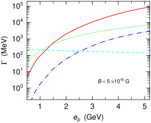
Figure 2: (Color online) Pionic decay width of protons versus the proton incident energy for $B=5\times 10^{18}$G. The decay width is averaged over the proton spin, and the Landau number is taken to be a maximum. The solid and dot-dashed lines represent the decay widths of the proton with and without the AMM, respectively. The dashed and dotted lines indicate the results in the semi-classical approaches of Refs. TK99 and in BDK95 , respectively.

When the proton energy is $e_{p}=1$ GeV, the semi-classical approach gives $\Gamma_{sc}\approx 180$  MeV in Refs. TK99 and 210 MeV in BDK95 . These values are close to the maximum value of the pionic width of the proton with the AMM when $s_{i}=-1$. However, the AMM is not taken into account in the semi-classical calculations, and the results in the semi-classical approach should be compared with our results without the AMM. In addition, the expression of Ref. BDK95 is derived with the condition, $\chi\gg 1$, which is not consistent to the present condition, $\chi\approx 0.06-0.5$. So, the decay width in the microscopic approach is much smaller than that in the semi-classical approach for the case without the AMM. Therefore, the AMM contribution, which is unique in the quantum mechanical approach, is vital for pion synchrotron radiation, particularly, in the limit of small curvature radii.

As the proton energy increases, the decay widths in the microscopic framework drastically increase, while those in the semi-classical approach increase more gently. In the semi-classical calculation one assumes that the Landau level number is very large. For example, in Ref. BDK95 , they take the limit, $n_{i}\rightarrow\infty$. In Fig.2, on the other hand, the maximum Landau is taken to be $n_{max}\approx 20-700$, which is too small for the semi-classical approximation. Thus, the semi-classical calculation is not justified based upon the present condition. However, the AMM contribution turns out to significantly increase the pion emission in the limit of a strong magnetic field.

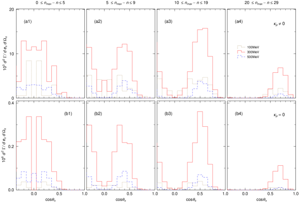
Figure 3: (Color online) The differential proton pionic decay width versus the polar angle of pion emission. The widths are averaged over the initial Landau levels, $0\leq n_{max}-n_{i}\leq 4$ (a1,b1), $5\leq n_{max}-n_{i}\leq 9$ (a2, b2), $10\leq n_{max}-n_{i}\leq 19$ (a3, b3) and $20\leq n_{max}-n_{i}\leq 29$ (a4, b4). The AMM is included in the upper panels (a1$-$4), and not included in the lower panels (b1$-$4). The emitted pion energies are taken to be $100$ MeV (dotted lines), 300 MeV (solid lines) and 500 MeV (dashed lines).

In order to understand the angular distribution of emitted pions, in Fig. 3, we present the differential pionic decay widths of the proton, averaged over various initial Landau levels, $0\leq n_{max}-n_{i}\leq 4$ (a1,b1), $5\leq n_{max}-n_{i}\leq 9$ (a2, b2), $10\leq n_{max}-n_{i}\leq 19$ (a3, b3) and $20\leq n_{max}-n_{i}\leq 29$ (a4, b4). The AMM contribution is included in the upper panels (a1$-$a4), but not included in the lower panels (b1$-$b4). The emitted pion energies are taken to be $100$ MeV (dotted lines), 300 MeV (solid lines), 500 MeV (dashed lines). Because the differential decay width is discrete for each angle, we average the results over the polar angle in every angular bin with $\Delta\cos\theta_{\pi}=0.1$.

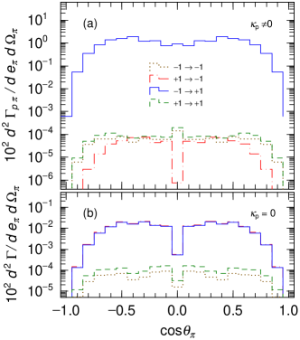
Figure 4: (Color online) The differential pionic decay widths of protons with (a) and without (b) the AMM included. The widths are averaged over initial Landau numbers, $0<n_{max}-n_{i}<9$. The solid, dot-dashed, dashed, and dotted lines represents the results when $s_{i}=-s_{f}=-1$, $s_{i}=-s_{f}=1$, $s_{i}=s_{f}=1$, and $s_{i}=s_{f}=-1$, respectively, where $s_{i}(f)$ indicates the initial (final) spin of the proton.

We should note that the angular distribution is symmetric between $\cos\theta_{\pi}<0$ and $\cos\theta_{\pi}>0$, so that we do not plot results for all $\cos\theta_{\pi}$. A pion produced from a proton with a higher Landau level $n_{i}$ is emitted more transversely, and the AMM effect shifts the pion emission to a more sideward direction when $0\leq n_{max}-n_{i}\leq 4$. If we consider that the emitted pion decays into 2$\gamma$s, it could affect the relativistic beaming of the energetic gamma rays from GRBs.

Next we examine the proton-spin condition for the pionic decay width. In Fig. 4 we give the initial and final spin-dependence of the proton differential pionic decay widths with (a) and without (b) the AMM. These widths are averaged over the initial Landau levels $0\leq n_{max}-n_{i}\leq 9$. The solid lines represent the results when the initial spin $s_{i}=-1$ and the final spin $s_{f}=1$. The dot-dashed, dashed and dotted line indicate cases for which $s_{i}=-s_{f}=1$, $s_{i}=s_{f}=1$, and $s_{i}=s_{f}=-1$, respectively.

When $\kappa_{p}=0$, the contributions from the spin-flip, $s_{i}=-s_{f}$, are about 100 times larger than those of the spin non-flip, $s_{i}=s_{f}$. Semi-classically the amplitude of the pion emission is proportional to $<\mbox{$\overline{\psi}$}_{N}\mbox{$\bm{\sigma}$}\cdot\mbox{$\bm{q}$}\psi_{N}>$. The pion emission along the $z$-direction is not allowed by energy-momentum conservation, and $<\mbox{$\overline{\psi}$}_{N}\sigma_{\pm}\psi_{N}>$ is the dominant contribution. Here, the spin-flip contributions become much larger than those from the spin non-flip reaction.

When the AMM is included, only the contribution from $s_{i}=-s_{f}=1$ is about 10,000 times larger than those of the other channels, and the non spin-flip contributions are not much different between those with and without the AMM.

As shown in Fig. 1 the AMM increases the decay width by 100 times for the case of $s_{i}=1=-s_{f}=1$, and decreases it for the case of $s_{i}=-s_{f}=-1$. When $s_{i}=-s_{f}=1$, the effects of the AMM and spin-flip are synchronized, and they enlarge the width by up to a factor of $10^{3}$. When $s_{i}=-s_{f}=1$, the two effects cancel and the width stays on the same order as that of the non spin-flip transition.

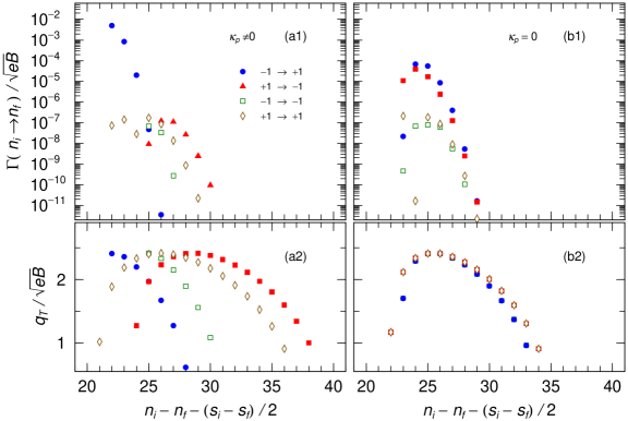
Figure 5: (Color online) Pionic decay widths of protons (a1, a2) and the pion transverse momentum (b1, b2) as functions of $n_{i}-n_{f}-(s_{i}-s_{f})/2$. The AMM is included in the left panels (a1, b1), and not included in the right panels (a2, b2). The initial Landau number is fixed to be $n_{i}+(1-s_{i})/2=45$.

Next, we examine contributions from the final Landau level. In Fig. 5 we show the width (a1 and a2) and the pion transverse momentum (b1, b2) as functions of $n_{i}-n_{f}-(s_{i}-s_{f})/2$, where the initial Landau number is fixed to be $n_{i}+(1-s_{i})/2=45$. The results are calculated with and without the AMM in the left (a1, b1) and right panels (a2 and b2), respectively.

Here, we note that the peak positions of the decay widths and the pion transverse momentum are the same. When $\kappa_{p}=0$, the peak position is almost independent of the initial and final spin. When the AMM is included, however, the peak position of the non spin-flip transition is the same as that without the AMM, but it is shifted to smaller values when $s_{i}=-s_{f}=-1$ and to larger values when $s_{i}=-s_{f}=+1$.

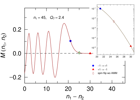
Figure 6: (Color online) The transition strength function $M(n_{i},n_{f})$, Eq. (23), when $n_{i}=45+(1+s_{i})/2$. The solid circle and triangle show the peak positions in the cases $s_{i}=-s_{f}=-1$ and $s_{i}=-s_{f}=1$, and the opened diamond indicates the case of the spin-flip $s_{i}=-s_{f}$ when $\kappa_{p}=0$.

In order to study the AMM effect more clearly, we next examine the transition strength $M(n_{i},n_{f})$ defined in Eq. (23). In Fig. 6 we show the $n_{f}$-dependence of $M(n_{i},n_{f})$ when $n_{i}=45+(1+s_{i})/2$. The solid circle and triangle in the inset represent the peak positions in the cases with $s_{i}=-s_{f}=-1$ and $s_{i}=-s_{f}=1$ with the AMM included. The open diamond indicates the case of a spin-flip $s_{i}=-s_{f}$ without including AMM.

$M(n_{i},n_{f})$ shows an oscillating behavior, but only the strength after the last peak contributes to the results. In this region the strength rapidly decreases with increases of $n_{i}-n_{f}$. A pion cannot be produced in the free kinematics, $B=0$, because of energy momentum conservation. Under the influence of a magnetic field, momentum conservation is not satisfied, so that a pion can be produced in the kinematical condition far from the free kinematics, where $M(n_{1},n_{2})$ rapidly decreases.

The AMM gives a repulsive potential for $s_{i}=-1$ and attractive for $s_{i}=1$. The transition with $s_{i}=s_{f}=-1$ introduces an additional energy to be consumed in the pion production. Thus, the difference between the initial and final Landau-levels is shifted toward a smaller number. In addition, the transition with $s_{i}=s_{f}=1$ reduces the production energy. In this kinematical region a small difference between the initial and final Landau-levels significantly changes the transition strength. Therefore, the AMM plays the important roles of increasing greatly the pionic decay width when $s_{i}=s_{f}=-1$ and to decrease it $s_{i}=s_{f}=1$.

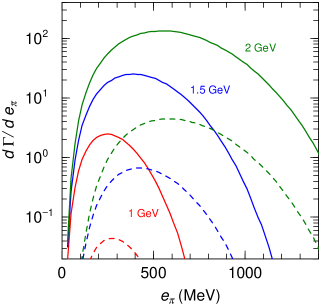
Figure 7: (Color online) The dependence of the proton decay width on the pion energy for a magnetic field of $B=5\times 10^{18}$ G. The solid and dashed lines represent the results with and without the AMM. The proton incident energies are taken to be 1, 1.5 and 2 GeV, respectively.

Next, we study the energy spectrum of the produced pions. We assume spherical symmetry in the momentum distribution of the initial protons and perform the angular integration of the differential decay width. In Fig. 7 we show the dependence of the proton decay width on the pion energy assuming a magnetic field $B=5\times 10^{18}$G and the proton energies of $e_{P}=1$, 1.5, 2GeV, respectively. The solid and dashed lines represent the results with and without the AMM, respectively.

As the proton energy increases, the decay width becomes larger, and the peak pion energy also increases. When the AMM is included, the peak height is about 59 times larger than that when it is neglected for $e_{p}=1$GeV, and its ratios are 36 for $e_{p}=1.5$GeV and 30 for $e_{p}=2$GeV; This difference between the peak height with the AMM and that without the AMM becomes smaller with increasing proton energy.

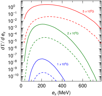
Figure 8: (Color online) The pion energy dependence of the proton decay width when the proton energy is $e_{p}=1$GeV. The solid and dashed lines represent results with and without the AMM. The magnetic fields are taken to be $1\times 10^{18}$G, $2\times 10^{18}$G, and $5\times 10^{18}$G. Results increase with an increase of the magnetic field strengths.

In Fig. 8 we show the dependence of the proton decay width on the pion energy for a proton energy $e_{p}=1$GeV with magnetic fields, $B=2\times 10^{18}$G, $5\times 10^{18}$G and $8\times 10^{18}$G. The solid and dashed lines represent the results with and without the AMM, respectively.

As the magnetic field increases, the decay width becomes larger, and the peak pion energy also increases. The peak height with the AMM included is about 93 times larger than that without the AMM for $B=1\times 10^{18}$G, and its ratios are 84 when $B=2\times 10^{18}$G, 56 when $B=5\times 10^{18}$G; the difference between the peak height with the AMM included and that without the AMM becomes larger as the magnetic field decreases.

As noted above, a pion can be produced in conditions far from that of free kinematics. As the magnetic field decreases, the breaking of momentum conservation becomes larger, so that the effect of the AMM becomes more significant.

IV Summary

In this work we have calculated the pion synchrotron radiation from high energy protons propagating in strong magnetic fields in a microscopic quantum field theoretical framework. We solved the Dirac equation in a strong magnetic field and obtained the proton propagator from its solution. Then, we derived the pionic decay width of the propagating proton in a fully relativistic and quantum mechanical way.

Our results turn out to be compatible to those obtained by classical approaches. In particular, we find out that the anomalous magnetic moment has a very large effect which enlarges the emission rate by about 50 times, when the proton energy is 1GeV and the magnetic field is $5\times 10^{18}$G. In actual magnetars the surface magnetic field is known to be of order $B\sim 10^{15}$G . In the present method we did not perform a calculation for such a magnetic field strength because of the large number of Landau levels involved: a few thousand to a few million.

As the magnetic field decreases, the AMM effect becomes larger. In a small magnetic field the decay width is very small, so that the proton energy must be larger to produce pions; if the semi-classical estimate is carried, the proton energy is expected to be at least about 100 GeV, and the maximum landau number should be a few hundred thousand. As the proton energy increases, on the other hand, the AMM effects diminish. Though it is not easy to estimate results for $B\sim 10^{15}$G, one expects the AMM effect to remain.

As for future studies, since the emitted pion can decay into two gammas with some angular dependence with respect to the magnetic field, the secondary produced gamma ray may affect the photons from GRBs. More detailed studies are necessary for further discussion of that additional effect. Since the pions as well as the photons (including vector mesons) may be emitted in strong magnetic fields, the weak $Z^{0}$ boson can also be produced from the propagating proton. This boson can decay into a pair of neutrinos. Detailed calculations regarding the neutrino pair production is also in progress.

Appendix A Proton Pionic Decay Width

In this section we show the detailed expressions of the proton pionic decay width, Eq. (17).

$$\frac{d^{3}\Gamma_{p\pi}/\sqrt{eB}}{dQ^{3}}=\frac{1}{8\pi^{2}Q_{0}}\left(\frac{f_{\pi}}{M_{\pi}}\right)^{2}\sum_{n_{f},s_{f}}\frac{\delta(E_{f}+Q_{0}-E_{i})}{4E_{i}E_{f}}R_{E}.$$ (24)

In the above equation $R_{E}$ is written as

$$R_{E} = \frac{1}{4}{\rm Tr}\left\{{\cal O}^{\dagger}_{\pi}\left[E_{f}\gamma_{0}+P_{fT}\gamma^{2}-P_{fz}\gamma^{3}+M_{N}+(\kappa_{p}/M_{N})\Sigma_{z}\right]\right.\left(A_{f}+\gamma_{5}\ooalign{\hfil/\hfil\crcr{$a$}}_{f}\right)$$ (30)

$$\left.\quad\times{\cal O}_{\pi}\left[E_{i}\gamma_{0}+P_{iT}\gamma^{2}-P_{iz}\gamma^{3}+M_{N}+(\kappa_{p}/M_{N})\Sigma_{z}\right]\left(A_{i}+\gamma_{5}\ooalign{\hfil/\hfil\crcr{$a$}}_{i}\right)\right\}$$

with $P_{i(f)T}=\sqrt{2n_{i(f)}+1-s_{i(F)}}$, and

$$A_{i(f)} = 1+\frac{s_{i}\kappa_{p}/M_{N}}{\sqrt{2n_{i(f)}+1-s_{i(F)}+M_{N}^{2}}}$$ (31)

$${\cal O}_{\pi} = \gamma_{5}\left\{\left[{\cal M}_{1}\frac{1+\Sigma_{z}}{2}+{\cal M}_{2}\frac{1-\Sigma_{z}}{2}\right]\left[\gamma_{0}Q_{0}-\gamma^{3}Q_{z}\right]\right.$$ (32)

$$\left.\quad-\left[{\cal M}_{3}\frac{1+\Sigma_{z}}{2}+{\cal M}_{4}\frac{1-\Sigma_{z}}{2}\right]\gamma^{2}Q_{y}\right\},$$

where

$${\cal M}_{1}={\cal M}\left(n_{i}+\frac{1-s_{i}}{2},n_{f}+\frac{1-s_{f}}{2}\right), {\cal M}_{2}={\cal M}\left(n_{i}-\frac{1+s_{i}}{2},n_{f}-\frac{1+s_{f}}{2}\right),$$

$${\cal M}_{3}={\cal M}\left(n_{i}+\frac{1-s_{1}}{2},n_{f}-\frac{1+s_{f}}{2}\right), {\cal M}_{4}={\cal M}\left(n_{i}-\frac{1+s_{i}}{2},n_{f}+\frac{1-s_{f}}{2}\right).$$

$R_{E}$ can be written explicitly as

$$R_{E}=\sum_{i<j}M_{i}M_{j}R(i,j).$$ (33)

with

$$R(1,1) = \frac{1}{2}\left\{[A_{i}A_{f}+s_{i}s_{f}(a_{i}\cdot a_{f})]\left[(P_{iL}\cdot P_{fL})(P_{iL}^{2}+P_{fL}^{2})-P_{iL}^{2}P_{fL}^{2}-(M_{N}+\kappa_{p}/M_{N})^{2}Q_{L}^{2}\right]\right.$$

$$~{}+s_{i}s_{f}(Q_{L}\cdot a_{i})(Q_{L}\cdot a_{f})\left[P_{iL}^{2}-P_{fL}^{2}+2(M_{N}+\kappa_{p}/M_{N})^{2}\right]$$

$$+(M_{N}+\kappa_{p}/M_{N})A_{f}s_{i}\left[(P_{iL}^{2}-P_{fL}^{2})(Q_{0}a_{i}^{z}-Q_{z}a_{i}^{0})-2Q_{L}^{2}(E_{i}a_{i}^{z}-P_{iz}a_{i}^{0})\right]$$

$$\left.+(M_{N}+\kappa_{p}/M_{N})A_{i}s_{f}\left[(P_{iL}^{2}-P_{fL}^{2})(Q_{0}a_{f}^{z}-Q_{z}a_{f}^{0})-2Q_{L}^{2}(E_{f}a_{f}^{z}-P_{fz}a_{f}^{0}\right]\right\},$$

$$R(2,2) = \frac{1}{2}\left\{[A_{i}A_{f}+s_{i}s_{f}(a_{i}\cdot a_{f})]\left[(P_{iL}\cdot P_{fL})(P_{iL}^{2}+P_{fL}^{2})-P_{iL}^{2}P_{fL}^{2}-(M_{N}-\kappa_{p}/M_{N})^{2}Q_{L}^{2}\right]\right.$$

$$~{}+s_{i}s_{f}(Q_{L}\cdot a_{i})(Q_{L}\cdot a_{f})\left[P_{iL}^{2}-P_{fL}^{2}+2(M_{N}-\kappa_{p}/M_{N})^{2}\right]$$

$$-(M_{N}-\kappa_{p}/M_{N})A_{f}s_{i}\left[(P_{iL}^{2}-P_{fL}^{2})(Q_{0}a_{i}^{z}-Q_{z}a_{i}^{0})-2Q_{L}^{2}(E_{i}a_{i}^{z}-P_{iz}a_{i}^{0})\right]$$

$$\left.-(M_{N}-\kappa_{p}/M_{N})A_{i}s_{f}\left[(P_{iL}^{2}-P_{fL}^{2})(Q_{0}a_{f}^{z}-Q_{z}a_{f}^{0})-2Q_{L}^{2}(E_{f}a_{f}^{z}-P_{fz}a_{f}^{0}\right]\right\},$$

$$R(3,3) = \frac{Q_{T}^{2}}{2}\left\{\left[P_{iL}\cdot P_{fL}+M_{N}^{2}-(\kappa_{p}/M_{N})^{2}\right](A_{i}A_{f}+s_{i}s_{f}a_{i}\cdot a_{f})-s_{i}s_{f}(Q_{L}\cdot a_{i})(Q_{L}\cdot a_{f})\right.\quad\quad\quad$$

$$\left.-(\kappa_{p}/M_{N})\left[Q_{0}(A_{f}s_{i}a_{i}^{z}-A_{i}s_{f}a_{f}^{z})-Q_{z}(A_{f}s_{i}0a_{i}^{0}-A_{i}s_{f}a_{f}^{0})\right]\right\}.$$

$$-\frac{Q_{T}^{2}}{2}M_{N}\left\{(E_{i}+E_{f})(A_{f}s_{i}a_{i}^{z}-A_{i}s_{f}a_{f}^{z})-(P_{iz}+P_{fz})(A_{f}s_{i}a_{i}^{0}-A_{i}s_{f}a_{f}^{0})\right\},$$

$$R(4,4) = \frac{Q_{T}^{2}}{2}\left\{\left[P_{iL}\cdot P_{fL}+M_{N}^{2}-(\kappa_{p}/M_{N})^{2}\right](A_{i}A_{f}+s_{i}s_{f}a_{i}\cdot a_{f})-s_{i}s_{f}(Q_{L}\cdot a_{i})(Q_{L}\cdot a_{f})\right.\quad\quad\quad$$

$$\left.-(\kappa_{p}/M_{N})\left[Q_{0}(A_{f}s_{i}a_{i}^{z}-A_{i}s_{f}a_{f}^{z})-Q_{z}(A_{f}s_{i}a_{i}^{0}-A_{i}s_{f}a_{f}^{0})\right]\right\}.$$

$$+\frac{Q_{T}^{2}}{2}M_{N}\left\{(E_{i}+E_{f})(A_{f}s_{i}a_{i}^{z}-A_{i}s_{f}a_{f}^{z})-(P_{iz}+P_{fz})(A_{f}s_{i}a_{i}^{0}-A_{i}s_{f}a_{f}^{0})\right\},$$

$$R(1,2) = P_{iT}P_{fT}\left\{Q_{L}^{2}\left[A_{i}A_{f}+s_{i}s_{f}a_{i}\cdot a_{f}\right]-2s_{i}s_{f}(Q_{L}\cdot a_{i})(Q_{L}\cdot a_{f})\right\},$$

$$R(1,3) = \frac{Q_{T}}{2}\left\{-\left[P_{iT}(P_{fL}\cdot Q_{L})+P_{fT}(P_{iL}\cdot Q_{L})\right]\left[A_{i}A_{f}+s_{i}s_{f}(a_{f}\cdot a_{i})\right]\right.$$

$$\quad+(P_{iT}+P_{fT})s_{i}s_{f}(Q_{L}\cdot a_{f})(Q_{L}\cdot a_{i})$$

$$\left.\quad+(P_{iT}-P_{fT})(M_{N}+\kappa_{p}/M_{N})\left[A_{f}s_{i}(Q_{0}a_{i}^{z}-Q_{z}a_{i}^{0})-A_{i}s_{f}(Q_{0}a_{f}^{s}-Q_{z}a_{f}^{0})\right]\right\},$$

$$R(1,4) = \frac{Q_{T}}{2}\left\{-\left[P_{iT}(P_{fL}\cdot Q_{L})+P_{fT}(Q_{L}\cdot P_{iL})\right]\left[A_{i}A_{f}+s_{i}s_{f}a_{f}\cdot a_{i}\right]\right.$$

$$\quad+(P_{iT}+P_{fT})s_{i}s_{f}(Q_{L}\cdot a_{f})(Q_{L}\cdot a_{i})$$

$$\left.\quad\quad+(P_{iT}-P_{fT})(M_{N}+\kappa_{p}/M_{N})\left[A_{f}s_{i}(Q_{0}a_{i}^{z}-Q_{z}a_{i}^{0})-A_{i}s_{f}(Q_{0}a_{f}^{z}-Q_{z}a_{f}^{0})\right]\right\},$$

$$R(2,3) = R(2,4)$$

$$= \frac{Q_{T}}{2}\left\{-\left[(P_{iL}\cdot Q_{L})P_{fT}+(Q_{L}\cdot P_{fL})P_{iT}\right]\left[A_{i}A_{f}+s_{i}s_{f}(a_{f}\cdot a_{i})\right]\right.$$

$$\quad\quad+(P_{iT}+P_{fT})s_{i}s_{f}(Q\cdot a_{f})(Q\cdot a_{i})$$

$$\left.\quad\quad+(P_{iT}-P_{fT})(-M_{N}+\kappa_{p}/M_{N})[A_{f}s_{i}(Q_{0}a_{i}^{z}-Q_{z}a_{i}^{0})-A_{i}s_{f}\left(Q_{0}a_{f}^{z}-Q_{z}a_{f}^{0}\right)]\right\},$$

$$R(3,4) = -Q_{T}^{2}P_{iT}P_{fT}\left(A_{i}A_{f}+s_{i}s_{f}a_{i}\cdot a_{f}\right),$$

where $P_{i(f)L}\equiv(E_{i(f)},0,0,P_{i(f)z})$ and $Q_{L}\equiv P_{iL}-P_{fL}=(Q_{0},0,0,Q_{z})$.

References

• (1) B. Paczyński, Acta. Astron. 41, 145 (1992).
• (2) For a review, G. Chanmugam, Annu. Rev. Astron. Astrophys. 30, 143 (1992).
• (3) R.E. Rothchild, S.R. Kulkarni and R.E. Lingenfelter, Nature 368, 432 (1994).
• (4) S. Mereghetti, Annu. Rev. Astron. Astrophys., 15, 225 (2008).
• (5) A.M. Soderberg , S.R. Kulkarni, , E. Nakar et al., Natur, 442, 1014 (2006).
• (6) N. Gehrels, C.L. Sarazin, P.T. O’Brien et al., Natur, 437, 851 (2005).
• (7) J.S. Bloom, J.X. Prochaska, D. Pooley et al., ApJ, 638, 354 (2006).
• (8) N.R. Tanvit, A.J. Levan, A.S. Fruchter et al., Natur, 500, 547 (2013).
• (9) A.I. MacFadyen, S.E. Woosley, ApJ, 524, 262 (1999).
• (10) A.I. MacFadyen, S.E. Woosley, A. Heger, ApJ, 550, 890 (2001).
• (11) S. Harikae, K. Kotake, T. Takiwaki, Y.-i Sekiguchi, ApJ, 720, 614 (2010).
• (12) S. Harikae, T. Takiwaki, J. otake, ApJ, 704, 354 (2009).
• (13) M.A. Hillas, Annu. Rev. Astron. Astrophys., 22, 425 (1984).
• (14) J. Aarons, ApJ, 589, 871 (2003).
• (15) K. Ioka, S. Razzaque, S. Kobayashi and P. Mészáros, ApJ, 633, 1013 (2005).
• (16) N. Gupta and B. Zhang, MNRAS, 380, 78 (2007).
• (17) M. Böttcher, and C. D. Dermer, ApJL, 499, L131 (1998).
• (18) T. Totani, ApJL, 502, L13 (1998).
• (19) Fragile, P. C., Mathews, G. J., Poirier, J., and T. Totani, APh 20, 591 (2004).
• (20) K. Asano and S. Inoue, ApJ, 671, 645 (2007) .
• (21) K. Asano, S. Inoue andP. Mészáros, ApJ, 699, 953 (2009).
• (22) A. Tokushita and T. Kajino, Astrophys. J. 525, L117 (1999).
• (23) V. Berezinsky, A. Dolgoy and M. Kachelriess, Phys. Lett. B 351, 261 (1995)
• (24) V.L. Ginzburg, and S.I. Syrovatskii, UsFiN, 87, 65 (1965).
• (25) V.L. Ginzburg, and S.I. Syrovatskii, Annu. Rev. Astron. Astrophys. 3, 297 (1965).
• (26) G.F. Zharkov, Sov. J. Nucl. Phys., 1, 17314 (1965).