DA white dwarfs from the LSS-GAC survey DR1: the preliminary luminosity and mass functions and formation rate

Abstract

Modern large-scale surveys have allowed the identification of large numbers of white dwarfs. However, these surveys are subject to complicated target selection algorithms, which make it almost impossible to quantify to what extent the observational biases affect the observed populations. The LAMOST (Large Sky Area Multi-Object Fiber Spectroscopic Telescope) Spectroscopic Survey of the Galactic anti-center (LSS-GAC) follows a well-defined set of criteria for selecting targets for observations. This advantage over previous surveys has been fully exploited here to identify a small yet well-characterised magnitude-limited sample of hydrogen-rich (DA) white dwarfs. We derive preliminary LSS-GAC DA white dwarf luminosity and mass functions. The space density and average formation rate of DA white dwarfs we derive are $0.83\pm 0.16\times 10^{-3}$ pc^-3 and $5.42\pm 0.08\times 10^{-13}$ pc^-3 yr^-1, respectively. Additionally, using an existing Monte Carlo population synthesis code we simulate the population of single DA white dwarfs in the Galactic anti-center, under various assumptions. The synthetic populations are passed through the LSS-GAC selection criteria, taking into account all possible observational biases. This allows us to perform a meaningful comparison of the observed and simulated distributions. We find that the LSS-GAC set of criteria is highly efficient in selecting white dwarfs for spectroscopic observations (80-85 per cent) and that, overall, our simulations reproduce well the observed luminosity function. However, they fail at reproducing an excess of massive white dwarfs present in the observed mass function. A plausible explanation for this is that a sizable fraction of massive white dwarfs in the Galaxy are the product of white dwarf-white dwarf mergers.

1 Introduction

White dwarfs (WD) are the typical endpoint of the evolution of most main sequence stars. Because nuclear reactions do not occur in their deep interiors, the evolution of WDs can be considered as a relatively simple and well understood gravothermal cooling process (Althaus et al., 2010a). Actually, the evolutionary cooling times are now very accurate (e.g. Renedo et al., 2010), providing a reliable way of measuring the WD cooling age from the temperature and surface gravity measured observationally. WDs are hence very useful tools in astronomy. For example, the WD luminosity function (LF) is an important statistical instrument which has been used not only to derive an accurate age of the Galactic disk in the solar neighborhood (Winget et al., 1987; Garcia-Berro et al., 1988; Fontaine et al., 2001) but also to constrain the local star formation rate (Noh & Scalo, 1990; Diaz-Pinto et al., 1994; Rowell, 2013). Moreover, the WD mass function (MF) has been successfully employed over the years as a tool to test the theory of stellar evolution, offering information on stellar mass loss. This function has also been used to study how the evolution of close binaries is able to produce low-mass WDs (Liebert et al., 2005), thus helping to asses the contribution of the distinct evolutionary scenarios in producing the current population of Galactic binaries in which one of the components is a WD. Finally, the WD age function (AF) is also a valuable tool for constraining the WD formation history (Hu et al., 2007).

With the advent of modern, large-scale surveys such as the Sloan Digital Sky Survey (SDSS; York et al., 2000) or the Super-Cosmos Sky Survey (Hambly et al., 2001), the size of the current observational WD samples has increased dramatically. This has allowed producing more accurate LFs, MFs and AFs (Harris et al., 2006; Kepler et al., 2007; Hu et al., 2007; De Gennaro et al., 2008; Rowell & Hambly, 2011). However, the major drawback of most studies is the complicated target selection algorithms, which incorporate observational biases that are almost impossible to quantify in numerical simulations that aim at reproducing the ensemble properties of the observed samples.

Significant observational efforts have also allowed to unveil the population of WDs within 20 pc of the Sun (Holberg et al., 2002, 2008; Giammichele et al., 2012). This sample is considerably less numerous than those mentioned above, however it is claimed to be reasonable complete and can therefore be considered as a volume (rather than magnitude) limited sample, which suffers effectively from no selection biases.

The LAMOST (Large Sky Area Multi-Object Fiber Spectroscopic Telescope) Spectroscopic Survey of the Galactic anti-center (LSS-GAC; Liu et al., 2014; Yuan et al., 2015) follows a well-defined selection criteria aiming at providing spectra for stellar sources of all colours in the Galactic anti-center (including WDs) so that they can be studied in a statistically meaningful way. LSS-GAC started operations in 2011 and will provide a significantly larger sample of WDs than those within 20 pc of the Sun. In this paper we derive preliminary observed LF, MF and AF of WDs identified within the first data release of LSS-GAC, and use a state-of-the-art Monte Carlo population synthesis code adapted to the characteristics of the survey to simulate the WD population in the Galactic anti-center. We apply the LSS-GAC selection criteria to the simulated samples, carefully evaluate all possible observational biases, and derive synthetic LFs, MFs and AFs. This exercise allows us to perform a meaningful comparison between the outcome of simulations and the observational data.

2 The LAMOST spectroscopic survey of the Galactic anti-center

LAMOST is a quasi-meridian reflecting Schmidt telescope located at Xinglong Observing Station in the Hebei province of China (Cui et al., 2012; Luo et al., 2012). The effective aperture of LAMOST is about 4 meters. LAMOST is exclusively dedicated to obtain optical spectroscopy of celestial objects. Each “spectral plate” refers to a focal surface with 4,000 auto-positioned optical fibers to observe spectroscopic plus calibration targets simultaneously, equally distributed among 16 fiber-fed spectrographs. Each spectrograph is equipped with two CCD cameras of blue and red channels that simultaneously provide blue and red spectra of the 4,000 selected targets, respectively.

The LSS-GAC is a major component of the LAMOST Galactic survey (Deng et al., 2012; Zhao et al., 2012). By selecting targets uniformly and randomly in ($r$, $g-r$) and ($r$, $r-i$) Hess diagrams (Yuan et al., 2015), the LSS-GAC main survey aims at collecting $\lambda\lambda$3,700 – 9,000 low resolution ($R\sim 1,800$) spectra for a statistically complete sample of $\sim 3$ million stars of all colours down to a limiting magnitude of $r=$17.8 mag (18.5 mag for limited fields), distributed in a contiguous sky area of over 3,400 deg² centered on the Galactic anti-center ($|b|\leq 30^{\circ}$, $150\leq l\leq 210^{\circ}$). The simple yet non-trivial target selection of the survey makes possible to study the underlying stellar populations for any given type of target, such as WDs. In addition to the main survey, the LSS-GAC also includes a survey of the M 31/M 33 area, targeting hundreds of thousands of objects in the vicinity fields of M 31 and M 33, and a survey of Very Bright (VB) plates, targeting over a million of randomly selected very bright stars ($r\leq 14$ mag) in the northern hemisphere during bright/grey nights.

Targets for the LSS-GAC main survey are selected for spectroscopic follow-up from the Xuyi Schmidt Telescope Photometric Survey of the Galactic anti-center (XSTPS-GAC) catalogue (Liu et al., 2014; Zhang et al., 2013, 2014). The XSTPS-GAC survey was initiated in October 2009 and completed in March 2011. Photometry in SDSS $g$, $r$ and $i$ bands was acquired with the Xuyi 1.04/1.20 m Schmidt Telescope located at the Xuyi station of the Purple Mountain Observatory, P. R. China. The XSTPS-GAC surveyed an area of about 5,400 deg², from ${\rm RA}\sim 3$ to 9^h and ${\rm Dec}\sim-10$ to +60^o to cover the LSS-GAC main survey footprint, plus an extension of $\sim 900$ deg² to the M 31, M 33 region to cover the LSS-GAC M 31/M 33 survey area. The resulting catalogues contain about 100 million stars down to a limiting magnitude of $r\sim 19.0$ mag ($10\sigma$), with an astrometric calibration accuracy of 0.1 arcsec (Zhang et al., 2014) and a global photometric calibration accuracy of $\sim$2 per cent (Liu et al., 2014, Yuan et al., in prep.).

For the LSS-GAC main survey, bright (B), medium-bright (M) and faint (F) plates are designated to target sources of brightness 14.0$<r\la$ 16.3 mag, 16.3 $\la r\la$17.8 mag and 17.8 $\la r\leq 18.5$ mag, respectively. During the Pilot (Oct. 2011 – Jun. 2012) and the first year Regular (Oct. 2012 – Jun. 2013) Surveys of LAMOST, a total of 1,042,586 [750,867] spectra of a signal to noise ratio (S/N) $\geq$ 10 at 7450Å  [S/N $\geq$ 10 at 4650Å] have been collected, including 439,560 [225,522] spectra from the main survey. Most of the stars are from the B plates.

The raw data were reduced with the LAMOST 2D pipeline (Version 2.6) (e.g. Luo et al., 2004), following the standard procedures of bias subtraction, cosmic-ray removal, 1D spectral extraction, flat-fielding, wavelength calibration, and sky subtraction. The LAMOST spectra are recorded in two arms, 3,700 – 5,900 Å in the blue and 5,700 – 9,000 Å in the red. The blue- and red-arm spectra are processed independently in the 2D pipeline and joined together after flux calibration. Flux calibration for the LSS-GAC observations is performed using an iterative algorithm developed at Peking University by Xiang et al. (2015), achieving an accuracy of about 10 per cent for the whole wavelength ranges of blue- and red-arm spectra. A detailed description of the target selection algorithm, survey design, observations, data reduction, and value-added catalogs of the first LSS-GAC data release is presented in Yuan et al. (2015). In the current work we only consider spectra obtained by the main LSS-GAC survey. A list including the names of the plates employed for the main survey is provided in Table A1 (see Appendix).

3 The LSS-GAC WD sample

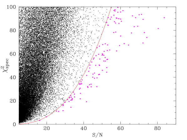
Figure 1: Reduced $\chi^{2}_{\mathrm{spec}}-\mathrm{S/N}$ distribution obtained by fitting one of our WD templates [$T_{\mathrm{eff}}$=14,000K, $\log(g)$=7 dex, see Fig. 2] to the entire LSS-GAC spectroscopic data base. Objects falling in the area defined by $\chi^{2}_{\mathrm{spec}}<0.002\times\mathrm{S/N}^{2.7}$ (red curve) are considered WD candidates (magenta dots).

In this section we describe our methodology for identifying WDs within the LSS-GAC spectroscopic data base. We do this following two independent but complementary routines. The first identifies WDs by $\chi^{2}$-template fitting all LSS-GAC spectra, the second selects WDs by applying a well-defined colour cut to the XSTPS-GAC photometric catalogue. We also estimate the spectroscopic completeness of the LSS-GAC WD sample.

3.1 The $\chi^{2}$-template fitting method

We use the $\chi^{2}$-template fitting method described by Rebassa-Mansergas et al. (2010) to identify LSS-GAC WDs. This routine was originally developed to search for SDSS WD-main sequence binaries (WDMS; Rebassa-Mansergas et al., 2010, 2012, 2013). However its mathematical prescription can be easily implemented to the LSS-GAC data for identifying single WDs. As the first step, a given WD template is used to fit the entire LSS-GAC spectroscopic data base and the resultant reduced $\chi^{2}_{\rm spec}$ values are recorded. Those $\chi^{2}_{\rm spec}$, together with the overall S/N ratios of the LSS-GAC spectra are represented in a 2D map and an equation of the form,

$$\chi^{2}_{\mathrm{max}}=a\times\mathrm{SN}^{b},$$ (1)

Figure 2: Four WD template examples used in this work. Effective temperature and surface gravity are indicated for each of them.

is defined so that all systems below this curve ($\chi^{2}_{\mathrm{spec}}<\chi^{2}_{\mathrm{max}}$) are considered as WD candidates, where $a$ and $b$ are free parameters defined for each template. An example is illustrated in Fig. 1. The form of Eq. (1) is defined to account for systematic errors between template and observed spectra, which become more important the larger the S/N is. The particular shape of the curve is carefully evaluated for each template as a compromise between the number of excluded/selected spectra. In other words, we aim at selecting as many WD candidate spectra as possible of similar spectral features as the templates used (note that, strictly speaking, the only free parameter we are considering in the fitting process is the normalization factor). However, the number of selected targets cannot be too large, as otherwise the automatization becomes useless.

The spectra of all WD selected candidates are then visually inspected and systems that are not WDs are simply excluded. This exercise is repeated for all WD templates considered. In this case, our templates are the result of adding artificial Gaussian noise to 45 DA (hydrogen-rich) carefully selected WD model spectra provided by Koester (2010) that cover a broad range of WD effective temperatures (6,000K-60,000 K) and surface gravities (7 $<\log\,g<$ 9 dex). The model spectra were binned to the LSS-GAC resolving power. Four of our considered WD templates are shown in Fig. 2. Obviously, using only DA WD templates restricts our search to hydrogen-rich WDs. However, as we show below (Section 3.3), the number of non-DA WDs currently observed by the LSS-GAC is rather small. Moreover, it has to be stressed that the presence of a small fraction of non-DA WDs does not seem to influence significantly the shape of the LF (Cojocaru et al., 2014).

As already mentioned, LSS-GAC spectra are the result of combining a blue and a red optical spectrum obtained from two separate arms. Given that single WDs are blue objects, in principle, the blue arm spectra alone should allow us to efficiently identify such stars. To investigate this, we separately applied the above described routine to all blue-arm LSS-GAC spectra as well as to all combined (blue- and red-arm) spectra and compared the results. We found that the number of identified WDs differed significantly. Specifically, we identified $\sim 30$ per cent more objects using the combined, blue plus red, spectra. Moreover, all WDs identified using only the blue-arm spectra were included in the list of targets found using the combined LSS-GAC spectra. The overall shape of the continuum spectrum is hence required for efficiently selecting single WDs. We found this effect to be most important when selecting WDs against hot (A) main sequence stars in which the strengths of the Balmer lines are similar. This was also the case when selecting WDs amongst low S/N ($\la 5$) spectra. For these two reasons, we decided to only consider the combined LSS-GAC spectra of S/N ratio above 5 in this work. This excluded 15,442 LSS-GAC spectra for which the default 2D pipeline (Section 2) failed to deliver usable red- and/or blue-arm spectra. It also excluded 622,112 spectra of S/N ratios below 5. This requirement is further supported by the fact that reliable stellar parameters (necessary for obtaining reliable LF, MF and AF) cannot be derived for low S/N ratio WD spectra (Rebassa-Mansergas et al., 2010). Thus, the total number of LSS-GAC spectra considered in this work was 306,600, of which 20,029 were selected as WD candidates by our $\chi^{2}$-template fitting method. A visual inspection revealed that 94 of those are genuine WDs, 81 of DA type (see Table 1). We also identified 26 WDMS binaries. With the exception of J080357.21+334138.6, these binaries are already included in the LAMOST WDMS binary catalogue by Ren et al. (2013, 2014).

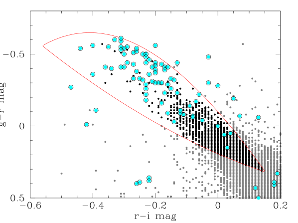
Figure 3: ($g-r$) versus ($r-i$) colour-colour plot illustrating the location of LSS-GAC DA white dwarf candidates (black solid dots within the colour cut defined by the red solid lines). The 92 confirmed LSS-GAC DAs are shown as cyan dots, others as grey dots The $g$ magnitudes of 22 LSS-GAC DA white dwarfs are found to be unreliable, which explains why these WDs are found outside the expected colour region (two of them beyond the displayed area).

3.2 The colour cut method

In the previous section we searched for DA WDs by $\chi^{2}$-template fitting all LSS-GAC spectra. Here we complement this with an independent strategy based on XSTPS-GAC $g$, $r$ and $i$ photometry (Section 2). This exercise relies simply on applying a well-defined cut to the XSTPS-GAC $g-r$ and $r-i$ colours (see Table 1 of Girven et al. 2011 and Fig. 3 of this paper). Girven et al. (2011) provide two additional colour cuts, using the $u$ and $z$ magnitudes respectively, however these are not used here because the XSTPS-GAC does not provide magnitudes in those filters. 16,824 sources fall within the area defined by our cut and visual inspection of spectra of those targets confirms 78 as WDs, of which 70 are DAs — see Table 1. The vast majority of the remaining targets are single A, F main sequence stars whose colours overlap with those of cool WDs. The contamination by quasars is negligible as these sources are generaly too faint to be observed by the LSS-GAC survey. 63 (57) of these 78 (70) WDs (DAs) are already discovered following the above described $\chi^{2}$-template fitting method. Thus, the colour method adds 15 new objects (13 of which are DAs) to our sample. The total number of LSS-GAC WDs thus raises to 105, and among them we classify 90 as DA WDs (Table 1). The complete LSS-GAC DA WD sample is provided in Table A2 (see Appendix).

Two important conclusions can be drawn from the above exercise. First, the $\chi^{2}$-template fitting method failed to identify $\sim 15$ per cent of the whole LSS-GAC DA WD sample. Visual inspection of the spectra of those systems revealed that they were either of low S/N ratios ($\sim 5-6$ in the blue-arm spectra), or were subject to artifacts of a bad flux calibration/merging of the two-arm (blue plus red) spectra, or a combination of both. Although those effects clearly affect the identification of DA WDs when applying the $\chi^{2}$-template fitting method, they do not influence the colour selection of DA WDs. Secondly, the DA WD colour cut we applied missed $\sim 22$ per cent of the whole DA WD sample identified. A closer inspection revealed the $g$ magnitudes of these targets to be unreliable. This caused those objects to fall far from the colour locus expected for DA WDs (see Fig. 3).

Table 1: Number of WDs (including DAs, DBs, etc.) and DAs alone identified by the $\chi^{2}$-S/N template fitting and colour methods, in common by the two methods, independently by each method, and missed by both methods. The total number of LSS-GAC WDs and DAs are provided in the last row.

	$N_{\rm WD}$	$N_{\rm DA}$
$\chi^{2}$-S/N method	94	81
Colour method	78	70
Common by both	63	57
$\chi^{2}$-S/N method alone	27	20
Colour method alone	15	13
Missed by both	2	2
Total	107	92

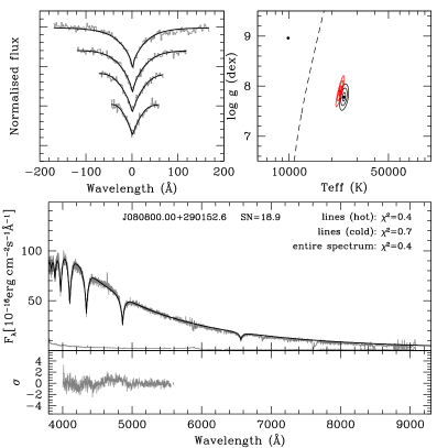
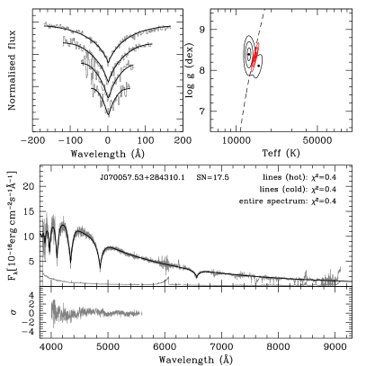
Figure 4: Spectral model fits to two DA WDs in our sample. Top row, 1st and 3rd panels: best-fit (black lines) to the normalised H$\beta$ to H$\epsilon$ (grey lines, top to bottom) line profiles. Top row, 2nd and 4th panels: 1, 3 and 6$\sigma$ $\chi^{2}$ contour plots in the $\mbox{$T_{\mathrm{eff}}$}-\log g$ plane. The black contours refer to the best line profile fit, the red contours to the fit of the entire (continuum plus lines) spectrum. The dashed line indicates the occurrence of maximum H$\beta$ equivalent width. The best “hot” and “cold” line profile solutions are indicated by black dots, the best fit to the entire spectrum (continuum plus lines) is indicated by a red dot. Bottom row, upper panels: the WD spectra and associated uncertaintied (grey lines) along with the best-fit model spectrum (black line) for the 4,000–5,500 Å wavelength range. The $\chi^{2}$ that result from the Balmer line fitting (cold and hot solutions) and the entire spectrum fitting are also indicated. Bottom row, lower panels. The residuals of the fit in the 4,000–5,500 Å  wavelength range. The $T_{\mathrm{eff}}$ and $\log g$ values listed in Table A2 are determined from the best Balmer line profile fit. The fit to the entire spectrum is only used to select between the “hot” and “cold” solutions of Balmer line profile fit (see also Fig. 5).

3.3 Spectroscopic completeness of the LSS-GAC DA WD sample

The spectroscopic completeness is defined as the fraction of DA WDs that we have identified compared to the total number of WDs observed by the LSS-GAC. It can be assumed that the DA WD spectroscopic sample is 100 per cent complete within the colour selection box defined by the $g-r$ and $r-i$ colours, as we have visually inspected every single spectrum within this region. There are 70 DA WDs in this colour box, of which 57 were found by the $\chi^{2}$-template fitting method (Table 1). The spectroscopic completeness of the $\chi^{2}$ method within the colour box is therefore 80 per cent. The number of DA WDs found by the $\chi^{2}$-template fitting method outside the colour box is 20 (Table 1). If we assume that the spectroscopic completeness of the $\chi^{2}$-template fitting method is not strongly colour dependent, then the total number of DA WDs we expect to lie outside the colour box is 20/0.8 = 25. The total number of DA WDs that could have been detected is therefore (70+25) = 95, and the overall spectroscopic completeness is (70+20)/95 $\simeq$ 95 per cent. The two independent methods we have used to identify LSS-GAC DA WDs, namely the $\chi^{2}$-template fitting method and the colour cut method, seem to complement each other very well and manage to identify the vast majority of DA WDs observed by the LSS-GAC survey.

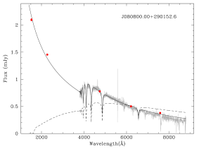
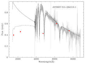
Figure 5: . Observed LSS-GAC spectra of the two DA WDs shown in Fig. 4 (gray), together with the best Balmer line model fits (black solid line for the hot solutions, black dashed line for the cold solutions). The GALEX near- and far-ultraviolet fluxes and the XSTPS-GAC optical fluxes (derived from the $g,r,i$ magnitudes) are shown as red solid dots. Left panel: the predicted ultraviolet and optical fluxes clearly select the hot solution of the Balmer fitting, in agreement with the solution preferred by fitting the entire LSS-GAC spectrum (Fig. 4, top row, second panel). Right panel: the GALEX ultraviolet fluxes are in good agreement with the cold Balmer line fit solution and thus clearly rule out the hot solution favoured by the fit to the entire LSS-GAC spectrum (Fig. 4, top row fourth panel). Note that in this particular case the $g$ XSTPS-GAC magnitude is found to be unreliable (Fig. 3).

An addional way to quantify the spectroscopic completeness is by cross-correlating our list with the LAMOST DA WD catalogues published by Zhao et al. (2013) and Zhang et al. (2013). Of the 16 DA WDs of Zhao et al. (2013), and 27 of Zhang et al. (2013) that fall in the area observed by LSS-GAC and have spectra of S/N ratios $\geq 5$ in both the red- and the blue-arm spectra, 15 and 26 are within our sample, respectively. Therefore, we have missed two DA WDs (Table 1). This exercise suggests a spectroscopic completeness of $\sim 94-96$ per cent for our sample, in good agreement with the above estimated value.

In Table A2 we include the two DA WDs that we have missed. This increases our LSS-GAC WD catalogue to 107 WDs. Of these, 92 are of the DA type (Table 1). Given that DA WDs are the most common ones – $\sim$85 per cent, see for example Kleinman et al. (2013) – and our final sample contains 92 DA WDs and seems to be highly complete, it can be said that the number of non-DA WDs currently observed by LSS-GAC is very small.

4 Stellar parameters and distances

We determine the stellar parameters following the fitting routine described by Rebassa-Mansergas et al. (2007). This relies on using the entire model grid of DA WDs of Koester (2010) to fit the normalised H$\beta$ to H$\epsilon$ line profiles of each WD spectrum for determining the effective temperature ($T_{\mathrm{eff}}$) and surface gravity ($\log g$). Two examples are illustrated in Fig. 4 (top row, first and third panels). Given that the equivalent widths of the Balmer lines go through a maximum near $\mbox{$T_{\mathrm{eff}}$}=13,000$ K (with the exact value being a function of $\log g$), $T_{\mathrm{eff}}$ and $\log g$ determined by fitting the Balmer line profiles are subject to an ambiguity, often referred to as “hot” and “cold” solutions. This implies that, at a given equivalent width, the Balmer lines of a cold and massive WD have the same profile as the Balmer lines of a hot and less massive WD (see Fig. 4, top row second and fourth panels). We break this degeneracy as follows. First, we fit the entire WD spectrum (continuum plus lines) with the same grid of model spectra used for fitting the Balmer lines (see bottom panels of Fig. 4). We used the 4,000-5,500 Å  wavelength range covered by the blue arm of the LSS-GAC spectra. This is because in some cases the combined LSS-GAC spectra are subject to artifacts of a bad merging of the blue plus red arm individual spectra. Since the continuum spectrum of a DA WD is mostly sensitive to $T_{\mathrm{eff}}$, the best-fit value from the entire spectrum indicates which of the two solutions is the prefered one. However, because of uncertainties in the flux calibration, the fit to the entire spectrum can only be used for breaking the degeneracy between the hot and cold solutions, rather than for obtaining a reliable set of stellar parameters. This in turn implies that the solution prefered by the best-fit to the entire spectrum may be subject to systemmatic uncertainties. Thus, in a second step the choice between hot and cold solution is further guided by comparing the ultraviolet GALEX (Galaxy Evolution Explorer; Martin et al., 2005; Morrissey et al., 2005) and optical XSTPS-GAC fluxes to the fluxes predicted from each solution (see two examples in Fig. 5). This exercise allows us to confidently select the correct solution for 75 of our 92 LSS-GAC DA white dwarfs. We use these 75 LSS-GAC DA white dwarfs as the sample of analysis in this work.

It has been shown that spectroscopic fits that use 1D model atmosphere spectra such as those employed in this work result in systematically overestimated surface gravities for WDs cooler than $\sim$12,000 K (Koester et al., 2009; Tremblay et al., 2011). We have thus applied the 3D corrections of Tremblay et al. (2013) to $T_{\mathrm{eff}}$ and $\log g$ determined above. We then interpolated the $T_{\mathrm{eff}}$ and $\log g$ values in the tables of Renedo et al. (2010) and Althaus et al. (2005, 2007, 2010b) to obtain masses, cooling ages, absolute $M_{\rm g}$, $M_{\rm r}$ and $M_{\rm i}$ and bolometric ($M_{\rm bol}$) magnitudes for our WDs. These cooling sequences provide absolute magnitudes in the $UBVRI$ system, which are converted into the $ugriz$ system using the equations of Jordi et al. (2006). Distances were finally obtained from the distance moduli of our targets, with the XSTPS-GAC $g,r,i$ magnitudes corrected for extinction using the 3D Galactic extinction map provided by Chen et al. (2014).

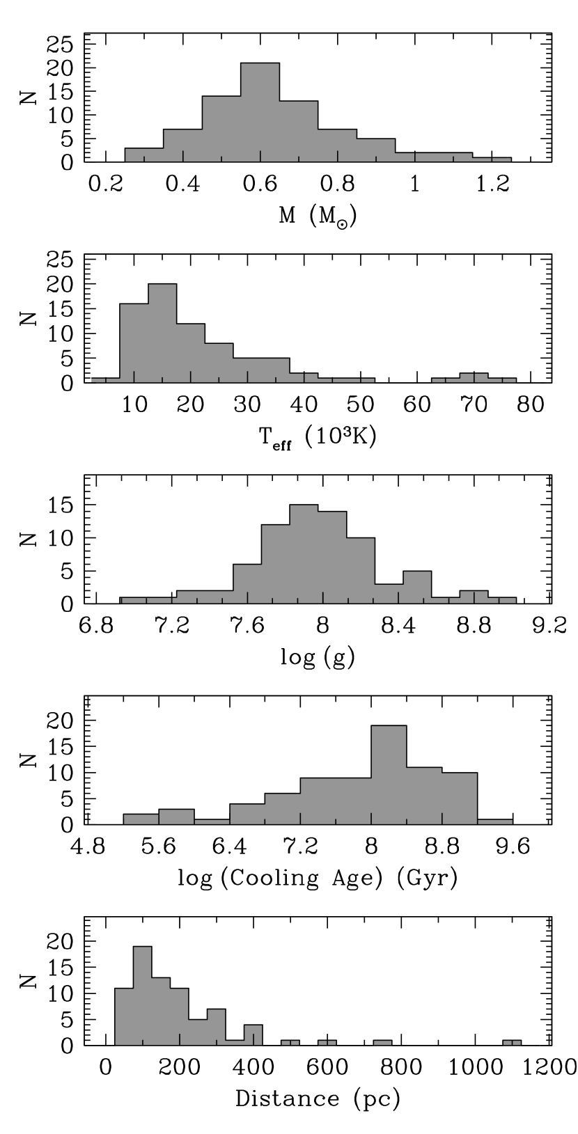
Figure 6: From top to bottom: mass, effective temperature, surface gravity, cooling age and distance distributions of the 75 LSS-GAC DA white dwarfs for which we are able to break the degeneracy between the hot and cold solutions obtained from fitting the Balmer lines of their spectra.

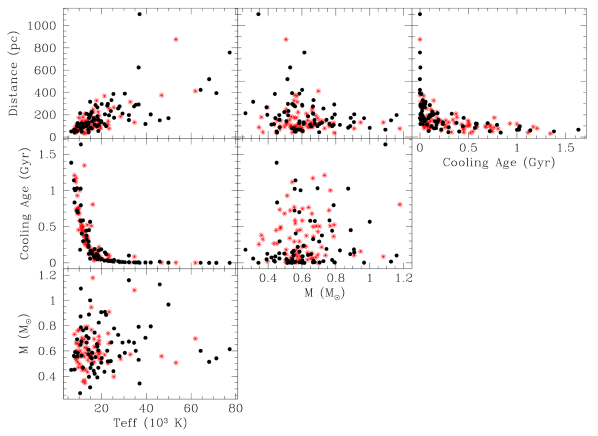
Figure 7: Correlations between the effective temperatures, masses, distances and cooling ages of the 75 LSS-GAC DA white dwarfs shown in Fig. 6 (black dots). We also show a typical realization of the Monte-Carlo simulations described in Section 6 (red stars). As can be seen the degree of overlap of the synthetic sample and the observational one is nearly perfect in all six panels.

The effective temperature, surface gravity, mass, cooling age and distance distributions of the 75 DA WDs for which we are able to break the degeneracy between the hot and cold solutions obtained by fitting the Balmer lines of their LSS-GAC spectra are shown in Fig. 6. Inspection of this figure reveals that the vast majority of LSS-GAC WDs are located at short distances ($\sim$50–300 pc). The mass and $\log g$ distributions broadly peak at 0.6 $M_{\odot}$ and $\log g=$ 8 dex respectively, features that have been observed previously in numerous studies (e.g. Koester et al., 1979; Holberg et al., 2008; Kepler et al., 2015). The effective temperatures are clustered between $\sim$ 10,000–15,000 K, and the majority of WDs have cooling ages between 0.01 and 1 Gyr. In Fig. 7 we show a grid of panels displaying the correlations between the effective temperatures, masses, distances and cooling ages (black dots) . We do not include the surface gravity here, as it is nearly equivalent to mass. It becomes clear that the higher the WD effective temperature the larger trends to be the distance, a clear selection effect indicating that cooler WDs need to be generally closer to us to be observed by the LSS-GAC. Also, hotter WDs trend to be further away, as otherwise they saturate the lower magnitude limit of the LSS-GAC. These effects are also noticeable when inspecting the relation between mass and distance: low-mass WDs are brighter and trend to be found at larger distances. It also becomes evident that, as a simple consequence of the WD cooling, the cooling ages decrease for increasing effective temperatures. Because of this there is also a tight relation between cooling age and distance, i.e. shorter cooling ages imply hotter WDs, therefore further distances. There is also a clear correlation between the cooling age and the distance, a quite natural behavior, since given that the mass distribution of WDs has a narrow peak around $0.6\,M_{\odot}$, the cooling ages and the effective temperature are very tightly correlated (see the leftmost central panel of this figure). Also shown in this figure is a typical realization of the Monte Carlo simulations described below (Section 6). It is quite apparent the high degree of overlap between the synthetic and the observed samples, indicating that our models reproduce with high fidelity the selection procedures, and the astronomical properties of the observed population.

From the above discussion it becomes clear that our observational sample and corresponding distributions are affected by selection effects typical of those incorporated by magnitude limited surveys. We correct for those observational biases in the next section.

5 The LSS-GAC DA WD luminosity and mass functions, and the DA WD formation rate

Magnitude limited surveys such as the LSS-GAC survey are affected by selection effects. Therefore, any parameter distribution that results from the analysis of a given observed population is subject to observational biases. The $1/V_{\rm max}$ method described in Schmidt (1968) and Green (1980) is aimed at removing these biases. In our case this is done calculating the maximum volume in which each of our WDs would have been detected given the magnitude limits of the LSS-GAC survey. This requires considering the lower and upper magnitude limits of each of the 16 spectrographs of each LSS-GAC plate. For each spectropgraph, the lower and upper magnitude limits define respectively the minimum ($d_{\mathrm{min}}$) and maximum ($d_{\mathrm{max}}$) distances (and therefore minimum and maximum volumes, $V_{\mathrm{min}}$ and $V_{\mathrm{max}}$) at which the considered WD would have been detected. The total maximum volume of a WD, $V_{\mathrm{WD}}$, is the sum over the individual maximum volumes obtained from each spectrograph – see also Hu et al. (2007); Limoges & Bergeron (2010):

$$V_{\mathrm{WD}}=V_{\mathrm{max}}-V_{\mathrm{min}}={\sum_{i=1}^{n_{\rm spec}}}\,\frac{\omega_{i}}{4\pi}\int_{d_{\mathrm{min}}}^{d_{\mathrm{max}}}e^{-z/z_{0}}~{}4{\pi}r^{2}dr=$$

$$=-\sum_{i=1}^{n_{\rm spec}}\frac{z_{0}\times\omega_{i}}{\left|\sin{b}\right|}\left[\left(r^{2}+\frac{2z_{0}}{\left|\sin{b}\right|}r+\frac{2z_{0}^{2}}{\left|\sin{b}\right|^{2}}\right)\!e^{-\frac{r\left|\sin{b}\right|}{z_{0}}}\right]_{d_{\mathrm{min}}}^{d_{\mathrm{max}}}$$ (2)

where $b$ is the Galactic latitude of the WD, and $\omega_{i}$ is the solid angle in steradians covered by each spectrograph (1.2 deg${}^{2}\times\pi^{2}/180^{2}$; $\sum_{i=1}^{n_{\rm spec}}\omega_{i}$ is the total area observed by the survey, also in steradians). The factor $e^{-z/z_{0}}$ takes into account the non-uniform distribution of stars in the direction perpendicular to the Galactic disc (Felten, 1976), where $z=r\times\sin(b)$ is the distance of the WD from the Galactic plane, and $z_{0}$ is the scale height, which is assumed to be 250 pc (Liebert et al., 2005; Hu et al., 2007). In the cases where two or more spectrographs observe the same region of sky, we consider the overlapping region with the largest volume, spanning between the smallest lower magnitude limit and the highest upper magnitude limit of the overlapping spectrographs.

Once $V_{\mathrm{WD}}$ is calculated for each WD in the observed sample the space density of WDs is simply obtained as $\sum 1/V_{\rm WD}=0.83\pm 0.16\times 10^{-3}$ pc^-3, where the sumation is over all the WDs in the sample. However, it has to be noted that the space density derived here represents an absolute lower limit, as we are able to derive reliable stellar parameters for only 75 of the 92 DAs in our sample. That is, we are considering just 81 per cent of the observed sample in the analysis. Moreover, the lowest effective temperature value among LSS-GAC DA white dwarfs is $\sim$6,500 K. WDs of lower effective temperatures are too faint to be detected by the survey, and are therefore not accounted for in our calculation of the space density. The space density as a function of the bolometric magnitude $M_{\rm bol}$, mass $M_{\rm WD}$ and cooling age $t_{\rm c}$ yield the WD LF, MF and AF, respectively. Each of these functions is analysed in the following sub-sections.

The $1/V_{\rm max}$ method described above can be also used to quantify the completeness of the observed sample, i.e. the percentage of WDs that are still missing because of selection effects after applying the $1/V_{\rm max}$ method. This completeness must not be taken as the spectroscopic completeness of the LSS-GAC sample, which is 95 per cent (see Section 3.3). If the sample is complete, then the average value $\langle V-V_{\mathrm{min}}\rangle/\langle V_{\mathrm{max}}-V_{\mathrm{min}}\rangle$ should be 0.5 (Green, 1980) (where $V$ is the volume of the WD as defined by its distance, i.e. the same as Equation (5), but integrating from 0 to $d$). In our case this quantity is 0.4, which corresponds to a completeness of 80 per cent. Of course, the above derived estimate of the completeness is within the context of the magnitude limits of the LSS-GAC survey, i.e. it does not account for populations of WDs that are too faint/rare to make it into the observed sample. Moreover, 19 per cent of the observed sample has not been considered in the analysis. If we were able to constrain the stellar parameters of these WDs, then the completeness would increase.

5.1 The luminosity function

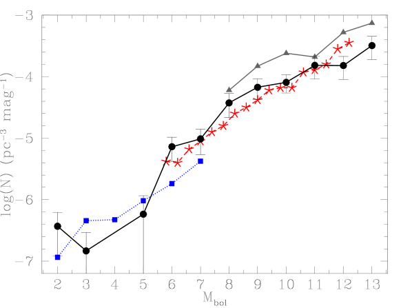
Figure 8: The LF of LSS-GAC DA white dwarfs and associated errors (solid black line and solid dots). For the sake of comparison we also show the LFs obtained by De Gennaro et al. (2008) (red dashed line and red stars), Torres et al. (2014) (blue dotted line and blue squares), and Giammichele et al. (2012) (solid grey line and grey triangles).

The LSS-GAC WD LF is shown in Fig. 8, its associated errors are calculated following Boyle (1989). For comparison we show the LFs obtained by De Gennaro et al. (2008) for the SDSS survey, Torres et al. (2014) for hot DAs in the SDSS (which supersedes the LF of Krzesinski et al. 2009), and Giammichele et al. (2012) for a local and volume limited sample of WDs. We note that two more LFs are available from the SDSS, provided by Harris et al. (2006) for photometric WD candidates, and by Hu et al. (2007) for Data Release 1 spectra of DA WDs. However, we do not show them in Fig. 8 because (1) the LF of Harris et al. (2006) assumes a constant $\log$ g $=8$ dex and very much resembles the one provided by De Gennaro et al. (2008) when considering DA WDs of the same $\log$ g value; (2) the work by De Gennaro et al. (2008) supersedes the analysis of Hu et al. (2007). Moreover, we decide not to show the LFs obtained by Liebert et al. (2005) for the Palomar Green Survey and Limoges & Bergeron (2010) for the KISO survey, as they also resemble the LF of De Gennaro et al. (2008) but contain considerably fewer objects. Because of completeness issues, the LF derived by Rowell & Hambly (2011) for WD candidates in the Super-Cosmos survey is not included neither. To avoid clustering of data in Fig. 8 we have also opted not to show the errors of all the above mentioned LFs.

Inspection of Fig. 8 reveals that, for $M_{\mathrm{bol}}\geq 6$ mag, the LF derived in this work is in good agreement with the LF of De Gennaro et al. (2008). The apparent disagreement between our LF and the one obtained by Giammichele et al. (2012) is likely due to the fact that the latter study includes all WDs (not only DAs) in a volume-limited local sample which does not presumably suffer from completeness issues, and therefore the space density is higher. For $M_{\mathrm{bol}}<6$ mag, our LF is also in broad agreement with that of Torres et al. (2014) for hot DAs. However, the number of LSS-GAC WDs falling in these bins is too small for a meaningful comparison between the two studies. It should be also noted that the WD LF actually continues to fainter magnitudes than those shown in Fig. 8, however we do not display those bins as these objects are too faint to be present in the LSS-GAC sample.

5.2 The mass function

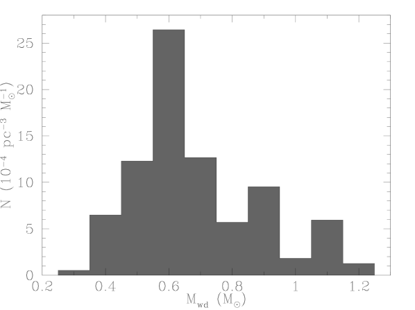
Figure 9: The MF of LSS-GAC DA white dwarfs.

The MF of the LSS-GAC WDs is displayed in Fig. 9. As expected, it shows a clear peak around 0.6 $M_{\odot}$. A relatively high percentage ($\sim$10 per cent) of low-mass ($<$0.5 $M_{\odot}$) WDs can also be seen. Traditionally, the existence of these low-mass WDs has been attributed to binary interactions (e.g. Liebert et al., 2005), and indeed it has been demonstrated that the majority of low-mass WDs are formed in binaries (Rebassa-Mansergas et al., 2011; Kilic et al., 2012). Therefore, DA WDs in those low-mass bins are expected to be part of binaries that contain unseen companions. Inspection of Fig. 9 also reveals a large fracion ($\sim$30 per cent) of massive ($\geq$0.8 $M_{\odot}$) WDs. A high-mass feature has also been regularly detected in a number of studies (e.g. Liebert et al., 2005; Kepler et al., 2007; Kleinman et al., 2013) and it has been claimed that it arises as a consequence of WD binary mergers. Population synthesis studies however do not predict more than $\sim$10 per cent of the entire WD population being the result of binary mergers (Han et al., 1994; Han, 1998; Meng et al., 2008; Toonen et al., 2012; García-Berro et al., 2012). Alternatively, a large number of high-mass WDs in the MF presented here may be the consequence of large uncertainties in the mass determinations (the mass errors of some of our objects are estimated to be $\ga 0.1-0.15$ $M_{\odot}$, which can move some objects across the corresponding mass bins). We will further discuss the large percentage of high-mass WDs identified in our MF in Section 7.4.

5.3 The formation rate of DA WDs

We now estimate the average DA WD formation rate following the method outlined by Hu et al. (2007). If the WD formation rate is assumed to be constant during the last Gyr, then the slope of the cumulative AF (see Fig. 10) can be considered as the average formation rate. Thus, we simply fit the cumulative AF with a straight line (the red dashed line in Fig. 10), and identify the slope of $5.42\pm 0.08\times 10^{-13}$ pc^-3 yr^-1 of the fit as the DA WD formation rate. Inspection of Fig. 10 reveals that, as expected, the maximum of the cumulative AF is $0.83\times 10^{-3}$ pc^-3, i.e. the total LSS-GAC DA WD space density.

Numerous studies in the past two decades have obtained WD formation rates. The most recent analysis (Verbeek et al., 2013) results in a birth rate of $5.4\pm 1.5\times 10^{-13}$ pc^-3 yr^-1, in excellent agreement with the value estimated here. The formation rates derived by Hu et al. (2007, $2.5-2.7\times 10^{-13}$ pc^-3 yr^-1), Liebert et al. (2005, $6\times 10^{-13}$ pc^-3 yr^-1), Holberg et al. (2002, $6\times 10^{-13}$ pc^-3 yr^-1) are also broadly consistent with the value estimated here. For comparison, earlier studies yield formation rates that are generally considerably higher (e.g. Green 1980, $20\pm 10\times 10^{-13}$ pc^-3 yr^-1; Weidemann 1991, $23\times 10^{-13}$ pc^-3 yr^-1; Vennes et al. 1997, $8.5\pm 1.5\times 10^{-13}$ pc^-3 yr^-1). This may be a consequence of the recent improvement in quality and size of WD data sets. Planetary nebulae birth rates are also found to be higher in general [Ishida & Weinberger 1987, $80\times 10^{-13}$ pc^-3 yr^-1; Phillips 2002, $21\times 10^{-13}$ pc^-3 yr^-1; Frew 2008, 8 $\pm$ 3 $\times 10^{-13}$ pc^-3 yr^-1]. The discrepancy has been discussed in detail in Liebert et al. (2005).

6 The LSS-GAC simulated DA WD luminosity, mass and cumulative age functions

In the previous sections we presented and characterised the sample of DA WDs identified within the data release 1 of the LSS-GAC. We also derived the DA WD space density, which has been used to construct the preliminary LF and MF of LSS-GAC DA WDs. Finally, we estimated the average DA WD formation rate from the DA WD cumulative AF. In this Section we simulate the LSS-GAC DA WD population and take advantage of the well-defined selection criteria employed by the LSS-GAC survey to evaluate the fraction of simulated WDs that would have been observed by the LSS-GAC survey. This will allow us to directly compare the ensemble properties of the observational data sets with the outcome of the simulations (see Section 7).

6.1 The population synthesis code

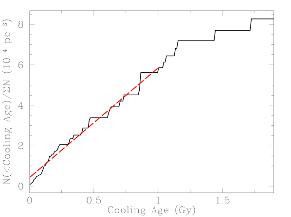
Figure 10: The LSS-GAC DA white dwarf cumulative age function. The slope of a straight line fit to the last Gyr (red dashed line) gives the average DA WD formation rate.

We provide here a brief description of our Monte Carlo WD population synthesis code, and of the changes done to adapt it to reproduce the LSS-GAC. A more complete and detailed description of the principal components of this method can be found in previous works (García-Berro et al., 1999; Torres et al., 2002; García-Berro et al., 2004).

Any Monte Carlo code has at its very core the idea of repeated random sampling, i.e. generating the statistical properties of data from known distributions, that is used to obtain the initial characteristics (mass, time of birth, initial position, kinematics, as well as other interesting quantities) of every star that will come to form part of the initial synthetic population. One main ingredient here is the pseudo-random number generator, for which we use the algorithm from James (1990). This produces a uniform probability density between $(0,1)$ with a repetition period of over $10^{18}$, more than sufficient for most practical purposes. The next important step is using adequate probability distribution functions for sampling the stellar properties. These distribution functions are crucial inputs that define each particular population. Thus, stellar masses are sampled using the initial mass function (IMF) of Kroupa (2001), a standard choice, in particular considering the alleged universal character of the IMF (Bastian et al., 2010). The moment at which each star is born ($t_{\mathrm{born}}$) is obtained in accordance with a star formation rate (SFR), assumed to be constant unless otherwise specified. The position of each star is randomly generated from a double exponential distribution of a constant Galactic scale height of $250$ pc and a constant scale length of $3.5$ kpc. The velocity distribution that we employ takes into account the differential rotation of the Galaxy, the peculiar velocity of the Sun and a scale height dependent dispersion law (Mihalas & Binney, 1981). Also, a metallicity value is assigned to each star according to a Gaussian metallicity distribution as presented in Casagrande et al. (2011).

In order to reproduce the LSS-GAC, stars are only generated in a cone delimited by $-30^{\circ}\leq b\leq 30^{\circ}$ in Galactic latitude and $150^{\circ}\leq l\leq 210^{\circ}$ in Galactic longitude (Section 2), with no restriction in terms of distance from the Sun. However, we define a test cone of up to 200 pc in length, in which we interactively examine the density of generated stellar mass until we reach a limit density value for the local stellar population (e.g. Holmberg & Flynn 2000). We scale this limit in order to obtain a final restricted WD sample of the same order as the observed one.

In a next step we set a 9.5 Gyr age for the thin disk ($t_{\mathrm{disk}}$) and interpolate the main sequence lifetimes ($t_{\mathrm{MS}}$) of the generated stars using the BaSTI grids according to stellar mass and metallicity (Pietrinferni et al., 2004). Knowing $t_{\mathrm{disk}}$, $t_{\mathrm{MS}}$ and $t_{\mathrm{born}}$, we can easily evaluate which of those stars have had time to become WDs. If that is the case the WD cooling age is simply given by $t_{\mathrm{c}}=t_{\mathrm{disk}}-t_{\mathrm{MS}}-t_{\mathrm{born}}$. Also, by knowing the mass of the WD progenitor we can compute the WD mass using an initial-to-final mass relation (IFMR), which will be further detailed in Section 6.2. WD luminosities, effective temperatures, surface gravities and $UBVRI$ and $M_{\mathrm{bol}}$ magnitudes are then obtained by interpolating the inferred WD masses and cooling ages along the following cooling tracks: for WD masses smaller than 1.1 $M_{\odot}$ and larger than 0.45 $M_{\odot}$ we use the CO sequences of Renedo et al. (2010) and Althaus et al. (2010b), while for WD masses above the upper value we employ the ONe tracks of Althaus et al. (2005) and Althaus et al. (2007). Finally, we convert the $UBVRI$ magnitudes into the $ugriz$ system using the equations of Jordi et al. (2006), taking into account the 3D Galactic extinction map of Chen et al. (2014) and the extinction coefficients of Yuan et al. (2013).

Table 2: The four models adopted in this work with the aim of reproducing the observed LSS-GAC DA WD population. Model 1 is our standard model.

Model	SFR	IFMR	Slope for the
			massive regime
1	Constant	Catalán et al. (2008)	0.10
2	Constant	Catalán et al. (2008)	0.06
3	Constant	Ferrario et al. (2005)	0.10
4	Bimodal	Catalán et al. (2008)	0.10

Some of the DA WD stellar parameters derived from the fits to the LSS-GAC spectra are subject to relatively large errors (Section 4). It is therefore necessary to account for those uncertainties in the simulated WD populations before comparing the synthetic and observational data sets. The effective temperature errors of the observed sample, which show a modest increase with increasing temperature, were fitted by a third order polynomial such that the error for relatively cool ($\sim 10,000$ K) WDs is about $300$ K, increasing to $\sim 1,000$ K for WDs as hot as $25,000$ K. We adopt this polynomial relation for deriving effective temperature errors of our simulated WDs. The observational errors of $\log\,g$ cluster around $\sim 0.2$ dex, and we take this value as the surface gravity uncertainty of the synthetic WDs. The values of effective temperature and surface gravity for each simulated WD are re-defined considering a random value within the error range defined for the two quantities. We then interpolate new values of mass, luminosity, cooling age, and bolometric and absolute magnitudes from the redefined $T_{\mathrm{eff}}$  and $\log g$ values. This results in, for example, an average error in mass of $\sim 0.1\,M_{\odot}$ for our simulated WDs. Photometric errors are also taken into account. They are directly derived from the photometric uncertainties associated with the XSTPS-GAC survey (Liu et al., 2014).

6.2 Models

As presented in Section 5, the observational sample exhibits several specific features that are clearly visible in the LF, MF and cumulative AF of the LSS-GAC WD sample (Figs. 8, 9 and 10). We attempt to reproduce those features by employing the above described population synthesis code.

Given the apparent excess of massive WDs seen in the MF (Fig. 9), we attempt to reproduce this feature focusing on three parameters of the simulations that can affect the final WD mass distribution, namely the SFR, the IFMR up to an initial mass of about 6 $M_{\odot}$ (the mass range of the zero-age main sequence for which WDs with CO cores are produced) and the slope of this (linear) relationship for the high-mass end (WDs with ONe cores). We start with our fiducial model, from now on called model 1, which uses a constant SFR, the piecewise linear IFMR introduced by Catalán et al. (2008) for the CO WD regime, and a slope of 0.1 for the massive regime (Iben et al., 1997).

We then consider three additional models, in which we vary only one of the above three parameters with respect to model 1. In model 2 we employ a slope of 0.06 for the IFMR of massive WDs (Weidemann, 2005). The reason for lowering the slope of the relationship to this value is to expand the range of initial masses that can produce massive WDs (over 1 $M_{\odot}$) in the hope of reproducing an excess. In order to ensure the continuity of the IFMR over the entire WD mass range and to be consistent with the upper CO WD mass limit, we consider that all stars with masses between 6 and 11 $M_{\odot}$ become WDs of core masses ranging from 1.1 to 1.4 $M_{\odot}$, which neatly gives this slope. Extending the mass range up to 1.4 $M_{\odot}$ is probably wrong, given that a WD that massive would most likely explode (Ritossa et al., 1999), but for the purposes of the current test is an acceptable assumption. Model 3 uses the curved IFMR from Ferrario et al. (2005) for the CO regime, which, according to these authors, results in a better agreement with the WD mass distribution as compared to when a linear fit is used. In model 4 we use the bimodal SFR of Rowell (2013), which has two broad peaks at around 2 and 7 Gyr ago. This SFR should favor an increase in the number of massive WDs during the last 2 Gyr given their shorter main sequence lifetimes. For each model we perform 10 individual realizations, and we compute the ensemble average of all the relevant quantities. A summary of the input parameters used for each model is given in Table 2.

6.3 The selection function

Once the synthetic DA WD samples have been obtained for the different models outlined in the previous Section, it becomes necessary to evaluate which of those synthetic WDs would have been observed by the LSS-GAC survey. Here, we describe how the selection process is performed.

The first step is to evaluate the effect of the LSS-GAC target selection criteria (Section 2). This is done independently for each of the 10 realizations of each model. For this purpose, the $g,r,i$ magnitudes of all WDs that are part of a given synthetic population are embedded within the XSTPS-GAC photometric catalogue and the selection criteria is then applied to the entire resulting population. The magnitude limits of the LSS-GAC survey are 14 mag $\leq r\leq$ 18.5 mag (Section 2), and within those limits the LSS-GAC criteria efficiently selects 80-85 per cent of the total simulated WD population, depending on the model. This fraction increases to 85-90 per cent if we consider 14 mag $\leq r\leq$ 18 mag. The high success rate of selecting WDs is not unexpected, considering that the LSS-GAC survey is specifically developed to efficiently target stars of all colours, including blue objects such as WDs (Section 2).

In a second step we evaluate which of the simulated WDs that are selected by the LSS-GAC criteria fall within the field of view (5 deg²) of the LSS-GAC plates actually executed (Table A1). If this is the case, an additional condition is that the simulated WDs are required to fulfill the magnitude limits of the plates/spectrographs, otherwise they would not have been observed. In practice, we consider the distances between the position defined by the right ascension and declination of each simulated WD and the central positions of the 16 spectrographs of the plate where the synthetic WD falls (also defined by their right ascensions and declinations) and evaluate whether or not the $r$ magnitude of the synthetic WD is within the magnitude limits of the nearest spectrograph. If all those conditions are fulfilled, we then consider the probability of a given target to be allocated a fibre (some fibres are used for sky observations). This probability is simply given by $N_{\mathrm{spec}}/(N_{\mathrm{spec}}+N_{\mathrm{sky}})$, and is generally $\sim$0.9. $N_{\mathrm{spec}}$ is the number of target spectra observed by the spectrograph, and $N_{\mathrm{sky}}$ is the number of fibres allocated for sky observations.

Table 3: The synthetic WD populations are passed through consecutive steps of filtering that gradually reduce the number of surviving objects. We show here an example for one of the 10 performed realizations of our standard model (Table 2). In the last two columns we indicate the percentage of WDs that survive respect to the previous step and the percentage of WDs that survive respect to the initial population, respectively.

	Filter	$N_{\mathrm{WD}}$	%	%
	Initial sample	3,874
	Initial sample within magnitude	2,132
	limits of the LSS-GAC
Step 1	Selection Criteria	1,748	82	82
Step 2	GAC plates + fibre allocation	192	11	9
Step 3	S/N $\geq$5	102	53	5
Step 4	Completeness + spectral fit	77	75	3.5

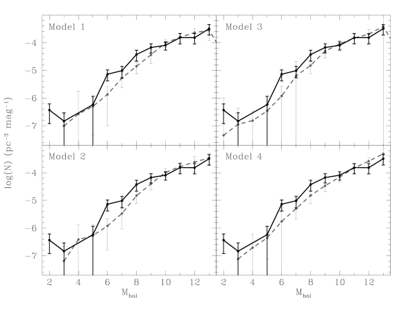
Figure 11: Simulated DA WD LFs (grey solid lines) resulting from the models considered in Section 6.2 (see Table 2). The observed LSS-GAC WD LF is shown as a black solid line.

If the synthetic WDs survive all the previously explained filtering process we consider the LSS-GAC survey would have observed them. Therefore, in a third step we consider the probability for each simulated WD to have a LAMOST spectrum of S/N ratio $\geq$ 5 in both the blue and red arms. For each synthetic WD we calculate the fluxes from their associated $g$ and $r$ magnitudes, add and subtract a 5 per cent of flux in each case and calculate the magnitudes that result from this exercise ($g_{+}$, $g_{-}$ and $r_{+}$, $r_{-}$; where the sufixes $+$ and $-$ indicate that we have added and subtracted the 5 per cent of the corresponding flux). We then consider all targets observed by the respective spectrograph (i.e. the spectrograph where the simulated WD falls) having $g_{-}<g<g_{+}$ and $r_{-}<r<r_{+}$, and calculate the median S/N ratio of their LSS-GAC spectra in the two bands. If no observed spectra are found satisfying the above magnitude ranges, or if one of the median S/N ratios is smaller than 5, the synthetic WD is then excluded from the analysis. This exercise takes into account nigh-to-night variations of S/N ratio that may arise e.g. from varying observing conditions, as the S/N is evaluated specifically for objects observed during the same night with the same plate/spectrograph, and of similar magnitudes as the simulated WD of concern.

Finally, in a fourth step we take into account the spectroscopic completeness of the observed sample (the fraction of LSS-GAC DA WDs that we have identified among all DA WDs observed) as well as consider the fact that we are not able to obtain reliable stellar parameters for 19 per cent of the observed sample. We have estimated a spectroscopic completeness of 95 per cent (Section 3.3). Therefore, we randomly exclude 5 per cent of all synthetic WDs that passed the previous filters. After this correction, we proceed by randomly excluding 19 per cent of the surviving systems.

In order to minimize the effects of the random exclusion of synthetic WDs, we repeat steps two to four 20 times per model realization. Given that each of the four models considered (Table 2) counts 10 realizations, we obtain 200 different final synthetic populations for each model. The number of simulated WDs that pass the entire selection process described above vary slightly from model to model (and realization to realization) and yields synthetic samples of 65–85 objects, similar to the number of WDs in the observed sample, 75 DA WDs. An example of how the number of synthetic WDs gradually decreases as they are passed through each of the filters of our selection process is shown in Table 3. In a final step we use bootstrapping techniques to produce synthetic samples of the same number of objects as the observed one.

The final LF, MF and cumulative AF for each model are the result of averaging 200 individual functions derived from each of the independent realizations. These are shown in Figs. 11, 12 and 14, respectively, where we also include the LF, MF and cumulative AF derived from the observational sample. A comparison of the synthetic and observed functions is presented and discussed in detail in the following Section.

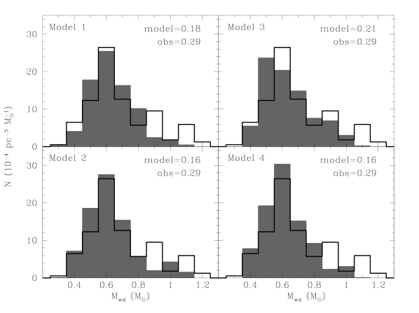
Figure 12: Same as Fig. 11 but for the MFs. The fraction of massive WDs ($>0.8$ $M_{\odot}$) for both the observed and the simulated samples are provided in the top right of each panel.

7 Discussion

In this section we compare the LFs, MFs and cumulative AFs (i.e. birth rates) that result from our numerical simulations to those derived observationally. Before comparing in detail the simulated and the observed distributions, we compare the WD populations obtained from each of the models employed here. We also estimate the number of DA WDs that the LSS-GAC will eventually observe.

7.1 The final expected number of LSS-GAC DA white dwarfs

The LSS-GAC selection criteria (Section 2) applied to our simulated WD populations results in $\sim$80-85 per cent of the synthetic DA WDs falling within the magnitude limits of the survey being selected for observations (Section 6.3). The total number of WDs generated by each model oscilates between 3,800 and 3,900, which reduces to 2,130–2,160 if we consider the magnitude limits of the LSS-GAC. This implies that, on average, $\sim$1,700-1,850 DA WDs could be potentially observed at the end of the survey, depending on the assumed model.

We have shown that $\sim$50 per cent of our synthetic DA WDs would have S/N$\geq$5 if observed by the LSS-GAC (see Table 3). This percentage is expected to increase up to $\sim$2/3 for the data release 2 (and further releases) of LSS-GAC spectra (private communication). The number of LSS-GAC DA white dwarfs expected to have spectra of S/N$\geq$5 at the end of the survey is thus $N_{\mathrm{DA}}=$(1,700–1,850$\,\,\,-\,\,\,N_{\mathrm{obs}})\times 2/3\simeq$ 1,070–1,170, where $N_{\mathrm{obs}}=92$, i.e. the number of currently observed DA WDs. Considering spectroscopic completeness and spectral fitting effects (Section 6.3, Table 3), which exclude $\sim 25$ per cent of the DA WD spectra with S/N$\geq$5, the final number of LSS-GAC DA white dwarfs with available and reliable stellar parameters at the end of the survey is expected to be $\simeq$800–875, i.e. approximately one order of magnitude higher than the current number of observed LSS-GAC DA white dwarfs with reliable stellar parameters.

7.2 Effects of observational uncertainties

We have employed four different models to simulate the WD population in the Galactic anti-center with the aim of constraining what set of assumptions (SFR, IFMR,…) fits better the observational data. As expected, the intrinsic properties of the simulated populations differed from model to model. However, these properties are altered when the observational uncertainties are incorporated (Section 6.1). For example, the simulated mass distributions become broader and lose detail, and more importantly, peak at larger values (e.g. the median of the distribution shifts from 0.57 $M_{\odot}$ to 0.60 $M_{\odot}$ for Model 2). Hence, the incorporation of observational uncertainties results in less prominent differences between the synthetic WD parameter distributions.

This effect is enhanced when we take into account the selection biases. In order to illustrate these effects together, we show in Fig. 7 the correlations between the effective temperatures, masses, cooling ages and distances for the synthetic population (red stars) and compare them to those obtained from the observational sample (black dots). For the seek of clarity we chose one typical realization of our Model 1, although very similar results are obtained for the other realizations and models. It becomes obvious that the model reproduces well the observational data, and that the correlations between the considered parameters follow the same pattern as the observational one (Section 4).

7.3 The luminosity function

Fig. 11 shows the LFs derived from our simulated samples, as well as that deduced from the observational data. The uncertainties in the simulated functions were derived in the same way as for the observed one (Section 5.1). The space density obtained for models 1, 2, 3 and 4, are $0.96\pm 0.19$, $0.98\pm 0.21$, $1.16\pm 0.20$ and $1.06\pm 0.20\times 10^{-3}$ pc^-3 respectively. Although these values are slightly higher than the space density derived from our observations ($0.83\pm 0.16\times 10^{-3}$ pc^-3, Section 5), they perfectly match within the error bars. It is evident that there is an overall good agreement (within the error bars) between the simulated and the observed LFs, except at $M_{\mathrm{bol}}$ 2 and 6 mag, where the observed LF predicts a considerably higher space density. It has to be noted, however, that the number of targets falling within bins of $M_{\mathrm{bol}}<7$ mag is small (18 per cent of the total observed sample). Hence, the observed LF in those high luminosity bins is subject to low number statistics and the apparent increase of the observed LF at those specific bins should be taken with some caution. A further inspection of Fig. 11 reveals that, because of the reasons explained above (Section 7.2), no model seems to have an obvious advantage in reproducing the observational data.

7.4 The mass function

After applying the LSS-GAC target selection criteria and the target selection process described in Section 6.3 to our simulated populations, the MFs yielded by all simulations are rather similar (Fig. 12). In addition, synthetic (single) WDs of masses as low as 0.35 $M_{\odot}$ are now possible as a consequence of incorporating observational uncertainties. This effect partly explains the apparent over-abundance of low-mass ($\la 0.45$ $M_{\odot}$) WDs in the observed MF (black solid line in Fig. 12). Alternatively, a relative large fraction of low-mass WDs in the observed sample could be the result of binary star evolution (Rebassa-Mansergas et al., 2011). The companions are likely to be cooler and/or more massive WDs, or low-mass late-type main sequence stars, although other exotic companions such as brown dwarfs cannot be ruled out.

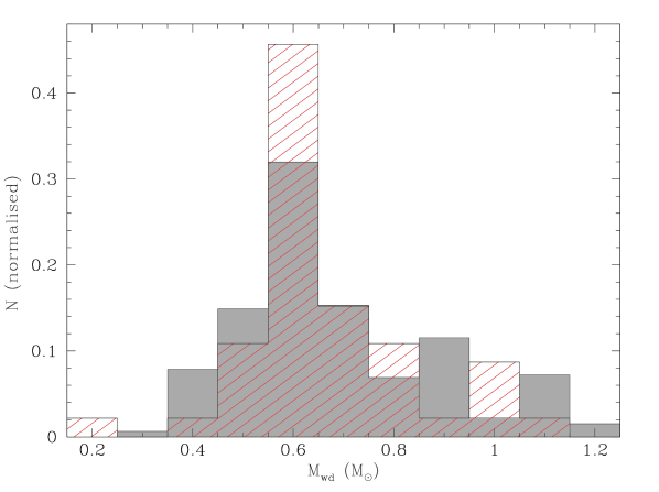
Figure 13: Normalised LSS-GAC DA white dwarf MF (gray) and normalised mass distribution of DA WDs from the local and volume-limited sample of Giammichele et al. (2012) (red dashed).

It is also clear that none of our models manages to completely reproduce the observed behaviour at high mass bins, i.e. the fraction of massive WDs ($>0.8$ $M_{\odot}$) relative to those of typical mass (0.6 $M_{\odot}$) is higher in the observed sample. We discuss possible scenarios leading to this feature below.

7.4.1 The initial-to-final mass relation

The currently available IFMRs have been derived from observational data that exhibit large scatter in the initial-to-final mass diagram (see for example Fig. 1 of Catalán et al., 2008). In one of our models we have investigated the effect of varying the slope of the IFMR for producing a wider range of massive WDs (see Section 6.2 and Table 2). We have also explored the effect of employing a curved IFMR (Ferrario et al., 2005). To further investigate the impact of the large scatter in the initial-to-final mass diagram to the simulated MF, two additional models (models 5 and 6) are developed that take into account the error bars of the IFMR of Catalán et al. (2008) so that the IFMR is virtually moved “up” in one model and “down” in the other model. The remaining free parameters of models 5 and 6 are the same as for our standard model (Table 2). The results show that the MFs obtained from these two models do not differ significantly from those shown in Fig. 12 and therefore are not able of reproducing the high-mass excess present in our observed MF.

7.4.2 S/N ratio and 3D model atmosphere correction effects

Two additional plausible explanations for the large fraction of massive WDs observed are effects of limited S/N ratios and 3D model atmosphere corrections.

The LSS-GAC spectra considered in this work have a minimum S/N ratio of 5. It is therefore possible that some systematic uncertainties in the WD stellar parameters result as a consequence of the relatively low S/N ratio of some WD spectra. This may lead to the masses of some WDs being overestimated. In order to investigate this possibility we re-derive the observed MF excluding all systems with spectra of a S/N ratio below 8. This leaves us with 52 DA WDs. We decided not to increase the S/N threshold to higher values because otherwise the number of massive (fainter and with systematically lower S/N ratios) WDs that would survive the cut would be severely reduced. The MF that results from this exercise does not differ significant from the one obtained using the full sample, and displays as well a large fraction of massive WDs. Therefore, S/N ratio effects are unlikely to be the cause of the excess of massive WDs observed.

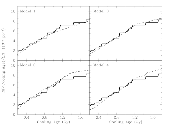
Figure 14: Same as Fig. 11 but for the cumulative AFs.

The DA WD sample analysed in this work includes cool WDs for which we have applied the 3D model atmosphere corrections to their stellar parameters deduced from 1D model atmosphere fitting: effective temperature, surface gravity, and hence mass. If those corrections are somehow incorrect, they may lead to an apparent overabundance of massive WDs. To explore this possibility we re-derived the MF excluding all WDs in our sample with an effective temperature below 13,000 K. This results in a sub-sample of 58 DA WDs. The MF deduced from this sub-sample again presents a clear overabundance of massive WDs. We therefore find that the overabundance of massive WDs is unlikely caused by the possible effects related to the 3D model atmosphere corrections.

7.4.3 Effective temperature and surface gravity error effects

The effective temperature and surface gravity errors obtained fitting the Balmer lines are not independent. The reason for this correlation is that the strength of the Balmer lines is largely determined by the ionization balance. That is, if the equivalent width of e.g. H$\beta$ is fixed, a higher assumed effective temperature will need a higher surface gravity, as the higher pressure is needed to compensate. The line shape is the second order effect, which determines where on the correlation line the best solution is. In order to ivestigate whether or not this effect may explain the excess of high-mass WDs observed, our simulations should have taken into account not only the errors in these quantites (see Sections 6.3 and 7.2), but also their correlation.

However, the strength of this correlation not only depends on the effective temperature range, but also the first order change of line strength disappears, and with it the correlation, near the maximum strength of the line. Moreover, the correlation is not always apparent for small errors. Hence, quantifying the correlation between the effective temperature and surface gravity errors is a notable endeaveour, which is beyond the scope of this paper. Thus, whether or not such a correlation may explain the apparent excess of massive WDs remains an open question.

7.4.4 WD+WD mergers

An exciting possible explanation for the excess of high-mass WDs in the observed MF is that a relatively large fraction of those stars are the result of mergers of two low-mass WDs (Marsh et al., 1997; Vennes, 1999). Although no population synthesis study hitherto predicts such a large fraction of high-mass WDs as the outcome of WD mergers (e.g. Han et al., 1994; Han, 1998; Meng et al., 2008; Toonen et al., 2012), this scenario has been adopted in some of the previous observational studies (e.g. Liebert et al., 2005; Giammichele et al., 2012). To further investigate this hypothesis we compare in Fig. 13 the normalised MF obtained in this work with the normalised mass distribution of DA WDs in the local, volume-limited sample of Giammichele et al. (2012). In becomes obvious that the peak at 0.6 $M_{\odot}$ is less pronounced in our normalised MF, an effect likely related to the fact that we are subject to larger observational uncertainties which broaden the distribution. Interestingly, whilst the high-mass peak in the normalised mass distribution of Giammichele et al. (2012) is found at 1 $M_{\odot}$, our normalised MF shows two apparent peaks at the 0.9 and 1.1 $M_{\odot}$ bins and reflects a scarcity of systems at the 1 $M_{\odot}$ bin. Although this discrepancy is likely due to our larger uncertainties, which are sufficient to shift objects across bins, both studies favour the hypothesis that an excess of massive WDs seems to exist.

If this excess of massive WDs may arise as a consequence of WD binary mergers, then the high merger rate implied by the observed excess of massive WDs may indicate a much more important role of the double-degenerate channel for the production of Type Ia supernovae (Wang & Han, 2012; Toonen et al., 2012). Analysing the expected merger rates of WDs based on our observations and comparing them to the observed rates of Type Ia supernovae thus seems to be a worthwhile exercise, and we will pursue this elsewhere. High-mass WDs that result from mergers are expected to be magnetic (García-Berro et al., 2012), therefore we may expect to find signs of magnetic fields in our massive WDs that should help test this hypothesis.

The large WD merger rate suggested by the current work indicates that an even larger number of close WD binaries may exist in the Galaxy that have not yet merged. Those close binaries could be a main source of gravitational waves to be detected by future facilities such as the space interferometer eLISA (Nelemans, 2013). Therefore, indirect support in favour of the merger scenario may be obtained by analysing the population of close double WDs that eLISA will discover.

7.5 The average DA WD formation rate

The cumulative AFs derived from our simulated populations are illustrated in Fig. 14, where the observed cumulative AF is also displayed. There is an overall good agreement between our simulations and the osbervations for coolinjg ages up to 1 Gyr, except perhaps for our model 4, which seems to systematically overestimate the space density for cooling age bins $<$0.4 Gyr (note that in model 4 we are employing a bimodal star formation rate). For cooling ages larger than 1 Gyr the discrepancies between the models and the observations arise due to the scarcity of WDs at those specific cooling ages.

Fitting the simulated cumulative AFs with a straight line (see Section 5.3) we derive average DA WD formation rates of 6.04$\pm$0.05, 6.42$\pm$0.05, 5.85$\pm$0.02 and 5.97$\pm$0.04 $\times 10^{-13}$ pc^-3 yr^-1 for models 1, 2, 3 and 4 respectively. These values agree with the average formation rate derived from our observations within the errors ($5.42\pm 0.08\times 10^{-13}$ pc^-3 yr^-1, Section 5.3). Because of the observational uncertainties (Section 7.2), we find that no model seems to have an obvious advantage in reproducing the observational data.

8 Summary and conclusions

The recently initiated LAMOST Spectroscopic Survey of the Galactic anti-center, the LSS-GAC, selects targets for spectroscopic observations following a well-defined criteria. This significant advantage over previous surveys has allowed us to present a well-characterised magnitude-limited sample of 92 LSS-GAC hydrogen-rich (DA) white dwarfs from the data release 1. Our catalogue is expected to be $\sim 95$ per cent complete. We have determined the stellar parameters (surface gravity, effective temperature and mass), absolute and bolometric magnitudes, and distances of 75 DA white dwarfs. Taking into account volume corrections we have derived an absolute lower limit for the space density of DA white dwarfs of 0.83$\pm 0.16\times 10^{-3}$ pc^-3. We have also obtained preliminary observed LSS-GAC DA white dwarf luminosity, mass and cumulative age functions. The luminosity function resembles those found in previous observational studies. The mass function reveals an excess of massive white dwarfs. Finally, the DA white dwarf formation rate derived from the cumulative age function is 5.42$\pm 0.08\times$10^-13 pc^-3 yr^-1, in good agreement with other recent studies.

We have simulated the DA white dwarf population in the Galactic anti-center using an existing Monte Carlo code adapted to the characteristics of the LSS-GAC. For this purpose, and specially aiming at reproducing the observed excess of massive white dwarfs, we have employed four different models. All those models take into account the observational uncertainties, both spectroscopic (i.e., we incorporate errors in the stellar parameters of our simulated white dwarfs based on the observational errors) and photometric. We find that the LSS-GAC criteria selects $\sim$80-85 per cent of all simulated white dwarfs with $14\leq r\leq 18.5$ mag (the magnitude limits of the survey) in each model, thus providing robust evidence for the high efficiency of LSS-GAC in targeting white dwarfs. Once the observational uncertainties have been taken into account in our simulations, the distribution of stellar parameters are similar for all models. We find that all our simulations reproduce well the observed luminosity function, however no particular model seems to fit better the data.

None of our considered models is able to reproduce the observed excess of massive DA white dwarfs. We have investigated possible explanations for this feature and concluded that a plausible scenario is that a sizable fraction of those massive white dwarfs are products of mergers of two initially lower-mass white dwarfs. If that is the case, then the white dwarf merger rate in our Galaxy is considerably higher than currently assumed. This may have important implications for the production of Type Ia supernovae via the double-degenerate channel.

Finally, it is important as well to emphasise that although our study represents an important step forward towards unveiling the underlying population of DA white dwarfs in the Galaxy, the size of the LSS-GAC sample is small, and that the stellar parameters we derived for some objects are subject to relatively large uncertainties. Forthcoming LSS-GAC data releases are expected to increase the number of DA white dwarfs by one order of magnitude. In addition, the quality of the LAMOST spectra will improve, which will reduce the uncertainties in the stellar parameter determinations. We will hence derive updated luminosity and mass functions and DA white dwarf formation rates at the end of the survey.

Appendix A Tables

Table 4: LSS-GAC plates, including associated right ascensions and declinations, used for observations. The date of observations are also included.

Date	Plate	RA	DEC	Date	Plate	RA	DEC
		[deg]	[deg]			[deg]	[deg]
2011-10-03	PA09B_keda1	63.79331	29.90206	2012-10-12	GAC090N33B1	90.06008	33.13693
2011-10-03	PA09B_keda2	63.79331	29.90206	2012-10-13	GAC072N32B1	72.32949	32.58819
2011-10-03	PA09M_keda1	63.79331	29.90206	2012-10-13	GAC072N32M1	72.32949	32.58819
2011-10-03	PA09M_keda2	63.79331	29.90206	2012-10-17	GAC083N27B1	83.98125	27.66235
2011-10-05	PA09F_keda1	63.79331	29.90206	2012-10-17	GAC083N27B2	83.98125	27.66235
2011-10-05	PA09M_keda1	63.79331	29.90206	2012-10-18	GAC085N33B2	85.74273	33.31455
2011-10-05	PA09M_keda2	63.79331	29.90206	2012-10-19	GAC080N32B1	80.00299	32.78560
2011-10-21	PA1B	45.87566	28.26991	2012-10-19	GAC080N32F1	80.00299	32.78560
2011-10-21	PB8B	91.59353	29.51241	2012-10-19	GAC080N32M1	80.00299	32.78560
2011-10-21	PB8M	91.59353	29.51241	2012-10-24	GAC051N24B1	51.07698	24.72406
2011-10-28	GAC_060N28_B1	60.35798	28.50189	2012-10-24	GAC051N24M1	51.07698	24.72406
2011-10-28	GAC_105N29_B1	105.02926	29.77213	2012-10-24	GAC100N32B1	100.68762	32.55887
2011-11-08	GAC_097N28_B1	97.59171	28.21211	2012-10-24	GAC100N32M1	100.68762	32.55887
2011-11-08	GAC_122N29_B1	122.39659	29.09308	2012-10-25	GAC086N24B1	86.98389	24.68684
2011-11-09	GAC_072N28_B1	72.31558	28.35083	2012-10-25	GAC086N24B2	86.98389	24.68684
2011-11-09	GAC_101N28_B1	101.18941	28.97093	2012-10-25	GAC086N24M1	86.98389	24.68684
2011-11-09	GAC_118N28_B1	118.33777	28.05199	2012-10-27	GAC090N26B1	90.89135	26.52913
2011-11-10	GAC_089N28_B1	89.14070	28.94227	2012-10-27	GAC090N26B2	90.89135	26.52913
2011-11-10	GAC_089N28_B2	89.14070	28.94227	2012-10-27	GAC102N27B1	102.29246	27.19037
2011-11-10	GAC_089N28_B3	89.14070	28.94227	2012-10-27	GAC113N27B1	113.05368	27.12516
2011-11-10	GAC_113N28_B1	113.63163	28.68658	2012-10-29	GAC078N26B1	78.08962	26.45461
2011-11-11	GAC_082N29_B1	82.41940	29.18646	2012-10-29	GAC098N33B1	98.42774	33.02404
2011-11-12	GAC_080N28_B1	80.84530	28.93676	2012-10-29	GAC113N26B1	113.98061	26.89574
2011-11-14	GAC_087N27_B1	87.66559	27.50503	2012-10-29	GAC117N24B1	117.32855	24.48873
2011-11-14	GAC_106N28_B1	106.85366	28.17669	2012-10-31	GAC097N26B1	97.23493	26.96746
2011-11-20	GAC_063022N281243_F1	97.59171	28.21211	2012-10-31	GAC114N33B1	114.58637	33.18676
2011-11-20	GAC_063022N281243_M1	97.59171	28.21211	2012-11-06	test_055N28_B1	55.32663	28.70276
2011-11-20	GAC_080935N290534_M1	122.39659	29.09308	2012-11-06	test_080N33_B1	79.75012	33.74839
2011-11-23	GAC_107N27_B1	108.98819	27.89742	2012-11-06	test_080N33_B2	79.75012	33.74839
2011-11-23	GAC_107N27_M1	108.98819	27.89742	2012-11-06	test_122N25_B1	122.55461	25.84448
2011-11-24	GAC_067N28_M1	72.31558	28.35083	2012-11-07	GAC049N32B1	49.14662	32.18402
2011-11-24	GAC_106N28_M1	106.85366	28.17669	2012-11-07	GAC049N32M1	49.14662	32.18402
2011-11-26	GAC_082N27_M1	87.66559	27.50503	2012-11-07	GAC069N25B1	69.84645	25.21827
2011-11-29	GAC_096N28_M1	100.33707	28.19664	2012-11-07	GAC107N32B1	107.68018	32.61873
2011-11-30	PB01B	47.40309	29.07708	2012-11-07	GAC117N27B1	117.47942	27.36318
2011-12-03	GAC_045N28_B1	45.87566	28.26991	2012-11-13	GAC073N32B1	73.87681	32.78394
2011-12-03	GAC_045N28_M1	45.87566	28.26991	2012-11-13	GAC073N32M1	73.87681	32.78394
2011-12-03	GAC_083N28_M1	89.14070	28.94227	2012-11-13	GAC102N32B1	102.42213	32.60676
2011-12-07	GAC_106N28_B1	106.85366	28.17669	2012-11-13	GAC102N32M1	102.42213	32.60676
2011-12-11	GAC_045N28_B1	45.87566	28.26991	2012-11-14	GAC098N33F1	98.42774	33.02404
2011-12-11	GAC_065N28_B1	68.65830	28.96115	2012-11-14	GAC098N33M1	98.42774	33.02404
2011-12-11	GAC_079N29_B1	82.52563	29.54832	2012-11-14	GAC121N33B1	121.03494	33.03074
2011-12-14	GAC_078N28_B1	80.84530	28.93676	2012-11-17	GAC079N24B1	79.38239	24.00968
2011-12-14	GAC_078N28_M1	80.84530	28.93676	2012-11-17	GAC079N24M1	79.38239	24.00968
2011-12-14	GAC_105N29_B1	105.02926	29.77213	2012-11-19	GAC058N31F1	58.01852	31.16858
2011-12-15	GAC_082N27_B1	87.66559	27.50503	2012-11-19	GAC121N33F1	121.03494	33.03074
2011-12-16	PB03B	56.15493	27.89745	2012-11-19	GAC121N33M1	121.03494	33.03074
2011-12-16	PB03M	56.15493	27.89745	2012-11-22	GAC049N27B1	49.98249	27.07113
2011-12-17	GAC_034118N284209_F1	55.32663	28.70276	2012-11-22	GAC089N24F1	89.23383	24.24969
2011-12-18	GAC_04h29_B1	61.75189	29.00130	2012-11-22	GAC089N24M1	89.23383	24.24969
2011-12-18	GAC_04h29_M1	61.75189	29.00130	2012-11-23	GAC083N24B1	83.37816	24.62881
2011-12-19	GAC_079N29_M1	82.41939	29.18646	2012-11-23	GAC104N26B1	104.69754	26.08108
2011-12-20	GAC_067N28_F1	72.31558	28.35083	2012-11-23	GAC120N25B1	120.23281	25.39284
2011-12-21	GAC_107N27_B1	108.98819	27.89742	2012-11-25	GAC117N31B1	117.75082	31.61353
2011-12-22	GAC_082N29_M1	82.52563	29.54832	2012-12-04	GAC041N29B1	41.91085	29.67853
2011-12-23	GAC_118N28_F1	118.33777	28.05199	2012-12-04	GAC117N24M1	117.32855	24.48873
2011-12-23	GAC_118N28_M1	118.33777	28.05199	2012-12-05	GAC065N31M1	65.04145	31.95317
2011-12-24	GAC_068N28_F1	68.65830	28.96115	2012-12-06	test_091N23_B1	91.70276	23.63860
2011-12-24	GAC_068N28_M1	68.65830	28.96115	2012-12-06	test_091N23_M1	91.70276	23.63860
2011-12-24	GAC_106N28_B1	106.85366	28.17669	2012-12-06	test_111N36_B1	111.07162	36.31091
2011-12-25	GAC_089N28_B3	89.14070	28.94227	2012-12-06	test_128N24_B1	127.87716	24.08111
2011-12-25	GAC_089N28_M3	89.14070	28.94227	2012-12-06	test_128N24_B2	127.87716	24.08111
2011-12-25	GAC_113N28_M1	113.63163	28.68658	2012-12-08	GAC074N27B1	74.97396	27.32560

Table 1: Continued.

Date	Plate	RA	DEC	Date	Plate	RA	DEC
		[deg]	[deg]			[deg]	[deg]
2011-12-26	GAC_047N29_B1	47.40309	29.07708	2012-12-08	GAC074N27M1	74.97396	27.32560
2011-12-26	GAC_091N29_B1	91.59353	29.51241	2012-12-09	GAC084N26B1	84.73905	26.61807
2011-12-26	GAC_091N29_M1	91.59353	29.51241	2012-12-09	GAC084N26M1	84.73905	26.61807
2011-12-27	GAC_105N29_M1	105.02926	29.77213	2012-12-09	GAC114N32B1	114.97536	32.00973
2011-12-28	GAC_108N27_M1	108.98819	27.89742	2012-12-21	GAC120N25M1	120.23281	25.39284
2011-12-31	PA06F	68.65830	28.96115	2012-12-22	GAC108N24B1	108.10991	24.12859
2011-12-31	PA06M	68.65830	28.96115	2013-01-04	test_076N27_B1	76.15819	27.69602
2012-01-02	PB06B	82.41939	29.18646	2013-01-04	test_076N27_M1	76.15819	27.69602
2012-01-02	PB06M	82.41939	29.18646	2013-01-04	test_094N28_B1	94.99571	28.42676
2012-01-03	GAC_068N28_B1	68.65830	28.96115	2013-01-04	test_126N31_B1	126.02454	31.30104
2012-01-03	GAC_101N28_M1	100.33707	28.19664	2013-01-05	GAC087N32B1	87.85729	32.12469
2012-01-04	GAC_063N29_B1	63.79331	29.90206	2013-01-05	GAC087N32M1	87.85729	32.12469
2012-01-04	GAC_106N28_M1	106.85366	28.17669	2013-01-06	GAC096N32B1	96.30344	32.27176
2012-01-11	GAC_050N29_B1	50.08484	29.04846	2013-01-06	GAC096N32M1	96.30344	32.27176
2012-01-12	GAC_045N28_B1	45.87566	28.26991	2013-01-07	GAC085N33M1	85.74273	33.31455
2012-01-12	GAC_100N28_B1	100.33707	28.19664	2013-01-07	GAC122N25B1	122.55461	25.84448
2012-01-13	GAC_061N29_B1	61.75189	29.00130	2013-01-07	GAC122N25M1	122.55461	25.84448
2012-01-14	PA09B1	89.14070	28.94227	2013-01-08	GAC086N24M2	86.98389	24.68684
2012-01-14	PA09M1	89.14070	28.94227	2013-01-09	GAC085N31B1	85.14961	31.35820
2012-01-14	PB02B	52.19438	30.37534	2013-01-09	GAC085N31M1	85.14961	31.35820
2012-01-15	PA01B	45.87566	28.26991	2013-01-11	GAC094N27M1	94.58662	27.21015
2012-01-15	PA09B1	89.14070	28.94227	2013-01-12	GAC054N25M1	54.29599	25.99110
2012-01-15	PB05B	70.09451	29.97223	2013-01-12	GAC078N26M1	78.08962	26.45461
2012-01-21	GAC_060N28_F1	60.35798	28.50189	2013-01-12	GAC109N30M1	109.51705	30.95587
2012-01-21	GAC_100N28_M1	100.33707	28.19664	2013-01-13	GAC080N33B2	79.75012	33.74839
2012-01-22	GAC_063N29_M1	63.79331	29.90206	2013-01-13	GAC080N33M1	79.75012	33.74839
2012-01-22	GAC_089N28_F1	89.14070	28.94227	2013-01-16	GAC045N26B1	45.47559	26.46235
2012-01-23	GAC_061N29_M1	61.75189	29.00130	2013-01-16	GAC055N32B1	55.61516	32.93923
2012-01-23	GAC_089N28_F2	89.14070	28.94227	2013-01-16	GAC065N31B1	65.04145	31.95317
2012-01-24	GAC_060N28_M1	60.35798	28.50189	2013-01-17	GAC040N27B1	40.86297	27.70715
2012-01-24	GAC_080N28_M1	80.84530	28.93676	2013-01-17	GAC105N24B1	105.60325	24.21545
2012-01-24	GAC_108N27_M1	108.98819	27.89742	2013-01-29	GAC058N25B1	57.85539	25.16293
2012-01-25	GAC_052N30_M1	52.19438	30.37534	2013-02-01	GAC076N33B1	76.53483	33.91869
2012-01-25	GAC_097N28_F1	97.59171	28.21211	2013-02-04	GAC046N25B1	46.36121	25.25517
2012-01-26	GAC_055N28_M1	55.32663	28.70276	2013-02-07	GAC054N25B1	54.29599	25.99110
2012-01-26	GAC_089N28_M2	89.14070	28.94227	2013-02-08	GAC046N25B1	46.36121	25.25517
2012-01-26	GAC_122N29_M1	122.39659	29.09308	2013-02-08	GAC062N26B1	62.70775	26.48095
2012-01-29	PA01M	45.87566	28.26991	2013-02-08	GAC109N31B1	109.37725	31.69805
2012-01-29	PA11F	106.85366	28.17669	2013-02-08	GAC109N31M1	109.37725	31.69805
2012-01-29	PB05M	70.09451	29.97223	2013-02-09	GAC072N28B1	72.31558	28.35083
2012-01-31	PB08M	91.59353	29.51241	2013-02-09	GAC094N27B1	94.58662	27.21015
2012-01-31	PB09B	100.33707	28.19664	2013-02-10	GAC110N25B1	110.86880	25.05053
2012-02-14	PA08F	124.98256	39.88470	2013-02-14	GAC053N32B1	53.75501	32.01677
2012-02-16	GAC_106N28_F1	106.85366	28.17669	2013-02-14	GAC114N32B1	114.97536	32.00973
2012-03-13	PA13B	129.34213	28.29440	2013-02-15	GAC076N30B1	76.06069	30.49459
2012-03-14	PB09B	100.33707	28.19664	2013-02-18	GAC053N32B1	53.75501	32.01677
2012-10-03	GAC080N33B101	79.75012	33.74839	2013-03-04	GAC_098N33_B1	98.42774	33.02404
2012-10-05	GAC054N25B1	54.29599	25.99110	2013-03-04	GAC_128N36_B1	128.34054	36.43643
2012-10-05	GAC067N27B1	67.33264	27.40422	2013-03-04	GAC_128N36_B2	128.34054	36.43643
2012-10-05	GAC089N24B1	89.23383	24.24969	2013-03-05	GAC078N26B1	78.08962	26.45461
2012-10-06	GAC085N33B1	85.74273	33.31455	2013-03-05	GAC108N24B1	108.10991	24.12859
2012-10-06	GAC085N33B2	85.74273	33.31455	2013-03-06	GAC089N28B1	89.14070	28.94227
2012-10-07	GAC081N30B1	81.78447	30.20860	2013-03-06	GAC089N28B2	89.14070	28.94227
2012-10-07	GAC081N30B2	81.78447	30.20860	2013-03-07	GAC082N33B1	82.00390	33.76370
2012-10-12	GAC056N24B1	56.20090	24.28947	2013-04-03	test_114N22_B1	114.41732	22.34006
2012-10-12	GAC056N24F1	56.20090	24.28947

Table 2: Names, coordinates, plate-spectrograph-fibre identifiers, XSTPS-GAC magnitudes and stellar parameters (effective temperature, surface gravity and mass) of the 92 DA LSS-GAC white dwarfs identified in this work.

Jname	RA	DEC	plateid	spid	fiberid	$g$	$r$	$i$	$T_{\mathrm{eff}}$	err	$\log(g)$	err	$M$	err
	[deg]	[deg]							[k]		[dex]		[M⊙]
J062647.53+264552.1	96.69805	26.76446	GAC_097N28_F1	5	220	17.53	17.64	18.03	27425	562	8.15	0.10	0.73	0.06
J070057.53+284310.1	105.23969	28.71946	GAC_105N29_M1	5	129	17.37	16.98	17.23	13173	462	8.27	0.16	0.78	0.11
J074722.19+295015.3	116.84244	29.83757	GAC_118N28_F1	16	27	18.19	17.83	18.05	15601	1150	7.78	0.28	0.50	0.15
J074850.71+301003.5	117.21131	30.16765	GAC_118N28_F1	16	228	18.27	17.89	18.11	-	-	-	-	-	-
J075106.48+301727.0	117.77698	30.29082	GAC_118N28_M1	11	169	15.65	15.92	16.39	32222	401	8.04	0.10	0.67	0.06
J074742.05+280945.6	116.92519	28.16266	GAC_118N28_F1	3	60	17.83	17.43	17.69	13234	286	8.18	0.09	0.72	0.06
J075251.35+271513.9	118.21396	27.25385	GAC_118N28_M1	5	171	16.72	16.73	17.15	23343	737	7.78	0.11	0.52	0.06
J034037.94+230304.2	55.15809	23.05117	GAC056N24F1	5	224	18.07	18.35	18.35	-	-	-	-	-	-
J051002.11+231541.0	77.50881	23.26140	GAC079N24B1	10	62	14.70	15.26	15.46	11134	131	7.89	0.11	0.56	0.07
J060027.42+234311.2	90.11425	23.71979	GAC089N24M1	8	7	16.98	16.98	16.98	8205	113	7.99	0.22	0.59	0.15
J033633.53+234938.7	54.13971	23.82742	GAC056N24F1	10	57	17.63	17.93	17.96	30419	1165	7.88	0.30	0.58	0.16
J073145.10+235352.9	112.93792	23.89802	GAC110N25B1	7	144	16.00	16.22	16.45	11736	372	7.75	0.27	0.47	0.16
J033900.07+242510.5	54.75028	24.41957	GAC056N24F1	3	53	18.01	18.49	18.52	17304	953	7.88	0.22	0.55	0.12
J055727.92+243558.8	89.36633	24.59967	GAC086N24M1	6	56	16.47	16.97	17.27	29387	567	8.04	0.13	0.67	0.08
J080230.40+244922.6	120.62665	24.82295	GAC120N25M1	4	119	17.66	17.75	17.87	9070	222	8.15	0.34	0.69	0.21
J054335.91+250410.8	85.89961	25.06966	GAC084N26M1	7	122	15.90	16.44	16.70	68101	4213	7.37	0.20	0.51	0.06
J034422.26+251453.3	56.09274	25.24813	GAC058N25B1	14	66	15.39	15.71	15.85	7931	101	7.74	0.29	0.45	0.18
J062159.50+252335.9	95.49790	25.39331	GAC094N27M1	7	21	17.56	17.62	17.70	11728	651	8.25	0.31	0.76	0.19
J032817.13+252853.5	52.07136	25.48152	GAC051N24M1	9	36	16.57	16.98	17.15	14132	944	8.00	0.16	0.61	0.10
J032854.06+252626.3	52.22527	25.44064	GAC051N24M1	9	35	18.06	17.73	17.54	-	-	-	-	-	-
J054613.53+255031.7	86.55636	25.84214	GAC_082N27_M1	2	249	17.33	17.62	17.78	-	-	-	-	-	-
J070950.16+255303.6	107.45899	25.88434	GAC_106N28_M1	1	184	17.10	17.63	17.94	77295	10207	7.64	0.42	0.61	0.16
J053727.46+260611.3	84.36441	26.10313	GAC084N26M1	4	135	16.76	17.17	17.33	15782	488	7.95	0.11	0.59	0.06
J064452.84+260947.7	101.22017	26.16326	GAC_100N28_B1	7	168	15.48	15.98	16.22	16910	671	7.60	0.16	0.42	0.07
J071223.81+260933.4	108.09919	26.15928	GAC_106N28_M1	7	226	16.85	17.24	17.41	14132	645	8.00	0.15	0.61	0.09
J055046.50+261220.3	87.69377	26.20563	GAC_082N27_B1	5	18	15.13	15.64	15.91	21289	814	7.60	0.14	0.43	0.06
J063532.49+261958.6	98.88537	26.33295	GAC_063022N281243_M1	7	221	16.63	17.17	17.47	34526	928	8.01	0.18	0.66	0.11
J063828.24+263359.6	99.61767	26.56656	GAC_100N28_B1	2	52	16.03	15.60	15.48	-	-	-	-	-	-
J063856.01+263022.5	99.73339	26.50626	GAC_100N28_B1	2	51	14.85	14.35	14.22	-	-	-	-	-	-
J025737.25+264047.9	44.40520	26.67997	GAC_045N28_M1	2	143	16.91	17.00	17.16	-	-	-	-	-	-
J063810.91+264040.9	99.54544	26.67802	GAC_100N28_B1	2	54	16.32	15.59	15.28	-	-	-	-	-	-
J063919.88+264102.6	99.83283	26.68405	GAC_100N28_B1	2	56	15.97	15.58	15.40	-	-	-	-	-	-
J070716.11+263857.5	106.81713	26.64930	GAC_106N28_M1	1	154	17.63	18.07	18.20	14899	783	7.29	0.19	0.31	0.06
J034605.50+264348.3	56.52290	26.73008	GAC_034118N284209_F1	7	240	17.54	17.95	18.26	22550	2127	7.95	0.35	0.60	0.21
J070755.01+265103.0	106.97921	26.85082	GAC_106N28_B1	5	12	15.53	15.86	16.01	15071	952	7.89	0.20	0.55	0.12
J070706.33+265756.7	106.77636	26.96574	GAC_106N28_M1	5	138	17.19	17.63	17.83	16910	564	8.21	0.14	0.74	0.09
J064743.70+270906.2	101.93207	27.15172	GAC_096N28_M1	6	25	16.00	16.59	16.90	41991	1207	8.21	0.12	0.79	0.07
J034409.58+271507.3	56.03992	27.25202	PB03M	5	172	16.02	16.52	16.75	19868	246	7.78	0.05	0.51	0.02
J054447.48+272032.0	86.19783	27.34223	GAC_082N27_M1	3	76	17.08	16.93	16.90	6459	56	7.75	0.14	0.45	0.07
J071520.95+273433.4	108.83731	27.57594	GAC_106N28_M1	6	192	17.93	18.01	18.12	-	-	-	-	-	-
J061540.92+275202.0	93.92048	27.86723	GAC094N27M1	15	229	16.47	16.91	17.20	46042	1008	8.82	0.11	1.13	0.05
J035123.16+280256.6	57.84651	28.04905	GAC_034118N284209_F1	6	169	17.75	18.11	18.51	32222	862	8.90	0.19	1.16	0.09
J061000.28+281426.9	92.50117	28.24081	test_094N28_B1	10	131	14.33	14.74	15.10	18542	62	7.97	0.02	0.60	0.01
J042945.25+282224.2	67.43856	28.37338	GAC_068N28_B1	3	248	14.60	15.21	15.52	39642	699	8.06	0.09	0.70	0.05
J074741.42+282104.9	116.92258	28.35137	GAC_118N28_F1	3	54	18.08	18.40	18.64	13284	2679	8.10	0.43	0.67	0.27
J080748.88+282626.4	121.95366	28.44067	GAC_080935N290534_M1	5	55	17.79	17.93	18.02	9356	256	7.97	0.51	0.58	0.32
J052147.24+283532.5	80.44682	28.59236	GAC_080N28_M1	4	198	17.50	17.73	17.86	10780	199	8.29	0.15	0.79	0.09
J030406.41+285143.2	46.02670	28.86200	GAC_045N28_M1	4	206	16.82	17.19	17.39	-	-	-	-	-	-
J030214.72+285707.4	45.56134	28.95206	GAC_045N28_M1	15	183	17.21	17.60	17.80	18120	1667	7.51	0.35	0.39	0.15
J053931.86+285456.7	84.88277	28.91574	GAC_079N29_M1	6	167	17.39	16.64	16.17	-	-	-	-	-	-
J042334.22+290205.7	65.89260	29.03492	GAC_068N28_F1	14	44	18.10	18.32	18.38	24443	2180	8.06	0.35	0.67	0.21
J080800.00+290152.6	122.00001	29.03127	GAC_080935N290534_M1	4	155	16.64	17.19	17.48	24163	600	7.78	0.09	0.52	0.04
J033134.40+291321.4	52.89335	29.22260	GAC_055N28_M1	14	111	17.14	17.40	17.55	14393	1093	7.56	0.26	0.39	0.12
J040403.73+291703.8	61.01555	29.28440	GAC_060N28_M1	9	165	17.73	17.80	17.73	-	-	-	-	-	-
J040842.17+292130.3	62.17569	29.35843	GAC_063N29_M1	10	223	17.06	17.01	16.97	7659	113	7.95	0.23	0.56	0.15
J071004.83+292402.8	107.52014	29.40079	GAC_107N27_B1	16	178	15.29	15.62	15.87	14089	732	7.94	0.18	0.57	0.11
J042435.27+293651.7	66.14697	29.61437	GAC_068N28_M1	14	104	17.29	17.52	17.69	36572	1719	8.22	0.30	0.79	0.18
J054658.08+293633.4	86.74200	29.60928	PA09M1	14	111	17.23	17.29	17.16	28064	789	7.84	0.16	0.56	0.08
J065740.34+300915.8	104.41810	30.15438	GAC_105N29_M1	3	134	17.14	17.08	17.06	7839	43	7.90	0.11	0.54	0.07
J071037.96+301146.4	107.65815	30.19622	GAC109N30M1	10	26	17.23	17.30	17.38	-	-	-	-	-	-
J030128.01+301536.6	45.36671	30.26016	GAC_045N28_B1	11	19	14.75	15.18	15.36	-	-	-	-	-	-
J071011.40+303041.7	107.54751	30.51158	GAC_106N28_M1	11	27	16.46	16.84	17.10	18756	594	8.33	0.12	0.82	0.08

Table 2: Continued.

Jname	RA	DEC	plateid	spid	fiberid	$g$	$r$	$i$	$T_{\mathrm{eff}}$	err	$\log(g)$	err	$M$	err
	[deg]	[deg]							[k]		[dex]		[M⊙]
J051624.54+303910.3	79.10227	30.65286	GAC080N32F1	2	118	17.84	18.14	18.33	21535	2125	8.46	0.37	0.91	0.21
J060113.75+304014.3	90.30730	30.67064	PA09M1	12	66	17.49	17.66	17.73	10939	330	8.12	0.31	0.68	0.20
J052038.36+304822.6	80.15984	30.80629	GAC_078N28_B1	16	139	15.38	15.68	15.88	15601	395	7.87	0.09	0.54	0.05
J033149.68+305944.9	52.95702	30.99581	GAC_052N30_M1	9	224	16.89	17.41	17.67	19868	306	8.46	0.06	0.91	0.04
J080039.67+305537.3	120.16529	30.92703	GAC121N33M1	2	118	17.44	17.84	18.18	25302	1399	7.58	0.20	0.44	0.08
J031430.60+310301.4	48.62749	31.05040	GAC049N32M1	5	42	17.20	17.61	17.82	18120	1669	8.03	0.38	0.64	0.23
J072438.30+310729.0	111.15957	31.12471	GAC109N30M1	9	238	17.35	17.51	17.69	10772	381	8.79	0.31	1.09	0.11
J075724.50+311310.3	119.35207	31.21953	GAC121N33F1	2	147	17.73	18.19	18.41	20098	741	7.85	0.14	0.54	0.07
J063058.95+312344.1	97.74564	31.39559	GAC096N32M1	6	239	17.24	17.53	17.76	15071	803	7.72	0.19	0.47	0.10
J055234.17+312401.6	88.14237	31.40045	GAC090N33B1	2	89	14.64	15.00	15.22	14228	176	8.15	0.03	0.70	0.02
J082705.52+313008.2	126.77302	31.50228	test_126N31_B1	9	22	15.36	15.92	16.32	71310	4547	7.44	0.22	0.54	0.06
J071603.19+315711.0	109.01331	31.95305	GAC109N30M1	15	11	17.72	17.91	17.86	-	-	-	-	-	-
J080602.45+315431.5	121.51019	31.90875	GAC121N33M1	8	185	17.25	17.80	18.11	22811	1761	7.78	0.28	0.52	0.15
J062856.67+320303.9	97.23611	32.05109	GAC098N33F1	5	193	17.77	18.31	18.75	36572	1334	7.71	0.24	0.53	0.11
J071451.13+320407.9	108.71306	32.06885	GAC109N30M1	15	76	15.89	16.44	16.79	49906	2195	8.49	0.18	0.97	0.09
J053712.39+321502.9	84.30162	32.25081	GAC085N31M1	15	243	16.70	16.96	17.19	16525	275	7.66	0.06	0.44	0.03
J042006.39+323305.0	65.02661	32.55138	GAC065N31B1	4	216	15.76	16.20	16.43	17912	544	8.06	0.11	0.65	0.07
J063100.30+324453.8	97.75127	32.74827	GAC100N32M1	14	38	16.16	16.76	17.09	64291	7505	7.70	0.41	0.60	0.18
J031336.68+325107.9	48.40285	32.85219	GAC049N32M1	15	248	17.29	17.40	17.52	10642	294	8.43	0.26	0.87	0.14
J031448.30+324916.3	48.70124	32.82120	GAC049N32M1	15	195	16.70	17.12	17.32	25595	915	8.24	0.13	0.78	0.08
J054709.65+324843.7	86.79021	32.81214	GAC085N33M1	8	2	16.72	16.31	16.13	-	-	-	-	-	-
J061736.85+325732.0	94.40353	32.95888	GAC096N32M1	14	173	16.49	16.97	17.20	35331	576	7.88	0.12	0.60	0.06
J080006.18+325738.1	120.02574	32.96058	GAC121N33F1	3	179	18.15	18.45	18.63	14393	1410	8.44	0.20	0.89	0.13
J030945.71+330025.0	47.44047	33.00694	GAC049N32M1	14	79	16.78	17.09	17.30	14899	1087	8.62	0.18	1.00	0.10
J075321.55+334308.1	118.33978	33.71892	GAC121N33F1	14	103	17.98	18.41	18.68	36996	2504	7.07	0.41	0.34	0.11
J055407.71+340348.0	88.53214	34.06334	GAC087N32M1	11	71	17.59	17.62	17.76	10409	188	7.19	0.40	0.27	0.17
J055019.78+350006.5	87.58242	35.00180	GAC085N33M1	12	184	16.31	16.64	16.91	18542	404	7.70	0.08	0.47	0.04
J051940.72+355137.1	79.91965	35.86031	GAC080N33M1	11	178	17.27	17.45	17.68	10656	174	8.08	0.21	0.65	0.14
J083400.13+365921.7	128.50056	36.98935	GAC_128N36_B2	4	206	16.05	16.09	16.14	9065	67	7.93	0.12	0.56	0.08
J084218.71+374859.4	130.57797	37.81649	GAC_128N36_B2	12	116	16.05	16.46	16.76	22037	1183	8.42	0.20	0.88	0.12

References

- Althaus et al. (2005) Althaus, L. G., García-Berro, E., Isern, J., Córsico, A. H., 2005, A&A, 441, 689
- Althaus et al. (2007) Althaus, L. G., García-Berro, E., Isern, J., Córsico, A. H., Rohrmann, R. D., 2007, A&A, 465, 249
- Althaus et al. (2010a) Althaus, L. G., Córsico, A. H., Isern, J., García-Berro, E., 2010a, A&A Rev., 18, 471
- Althaus et al. (2010b) Althaus, L. G., García-Berro, E., Renedo, I., Isern, J., Córsico, A. H., Rohrmann, R. D., 2010b, ApJ, 719, 612
- Bastian et al. (2010) Bastian, N., Covey, K. R., Meyer, M. R., 2010, Annual Review of Astronomy and Astrophysics, 48, 339
- Boyle (1989) Boyle, B. J., 1989, MNRAS, 240, 533
- Casagrande et al. (2011) Casagrande, L., Schönrich, R., Asplund, M., Cassisi, S., Ramírez, I., Meléndez, J., Bensby, T., Feltzing, S., 2011, A&A, 530, A138
- Catalán et al. (2008) Catalán, S., Isern, J., García-Berro, E., Ribas, I., 2008, MNRAS, 387, 1693
- Chen et al. (2014) Chen, B.-Q., et al., 2014, MNRAS, 443, 1192
- Cojocaru et al. (2014) Cojocaru, R., Torres, S., Isern, J., García-Berro, E., 2014, A&A, 566, A81
- Cui et al. (2012) Cui, X.-Q., et al., 2012, Research in Astronomy and Astrophysics, 12, 1197
- De Gennaro et al. (2008) De Gennaro, S., von Hippel, T., Winget, D. E., Kepler, S. O., Nitta, A., Koester, D., Althaus, L., 2008, AJ, 135, 1
- Deng et al. (2012) Deng, L.-C., et al., 2012, Research in Astronomy and Astrophysics, 12, 735
- Diaz-Pinto et al. (1994) Diaz-Pinto, A., Garcia-Berro, E., Hernanz, M., Isern, J., Mochkovitch, R., 1994, A&A, 282, 86
- Felten (1976) Felten, J. E., 1976, ApJ, 207, 700
- Ferrario et al. (2005) Ferrario, L., Wickramasinghe, D., Liebert, J., Williams, K. A., 2005, MNRAS, 361, 1131
- Fontaine et al. (2001) Fontaine, G., Brassard, P., Bergeron, P., 2001, pasp, 113, 409
- Frew (2008) Frew, D. J., 2008, Planetary Nebulae in the Solar Neighbourhood: Statistics, Distance Scale and Luminosity Function, Ph.D. thesis, Department of Physics, Macquarie University, NSW 2109, Australia
- García-Berro et al. (1999) García-Berro, E., Torres, S., Isern, J., Burkert, A., 1999, MNRAS, 302, 173
- Garcia-Berro et al. (1988) Garcia-Berro, E., Hernanz, M., Isern, J., Mochkovitch, R., 1988, Nature, 333, 642
- García-Berro et al. (2004) García-Berro, E., Torres, S., Isern, J., Burkert, A., 2004, A&A, 418, 53
- García-Berro et al. (2012) García-Berro, E., et al., 2012, ApJ, 749, 25
- Giammichele et al. (2012) Giammichele, N., Bergeron, P., Dufour, P., 2012, ApJ, 199, 29
- Girven et al. (2011) Girven, J., Gänsicke, B. T., Steeghs, D., Koester, D., 2011, MNRAS, 417, 1210
- Green (1980) Green, R. F., 1980, ApJ, 238, 685
- Hambly et al. (2001) Hambly, N. C., et al., 2001, MNRAS, 326, 1279
- Han (1998) Han, Z., 1998, MNRAS, 296, 1019
- Han et al. (1994) Han, Z., Podsiadlowski, P., Eggleton, P. P., 1994, MNRAS, 270, 121
- Harris et al. (2006) Harris, H. C., et al., 2006, AJ, 131, 571
- Holberg et al. (2002) Holberg, J. B., Oswalt, T. D., Sion, E. M., 2002, ApJ, 571, 512
- Holberg et al. (2008) Holberg, J. B., Sion, E. M., Oswalt, T., McCook, G. P., Foran, S., Subasavage, J. P., 2008, AJ, 135, 1225
- Holmberg & Flynn (2000) Holmberg, J., Flynn, C., 2000, MNRAS, 313, 209
- Hu et al. (2007) Hu, Q., Wu, C., Wu, X.-B., 2007, A&A, 466, 627
- Iben et al. (1997) Iben, Jr., I., Ritossa, C., García-Berro, E., 1997, ApJ, 489, 772
- Ishida & Weinberger (1987) Ishida, K., Weinberger, R., 1987, A&A, 178, 227
- James (1990) James, F., 1990, Computer Physics Communications, 60, 329
- Jordi et al. (2006) Jordi, K., Grebel, E. K., Ammon, K., 2006, A&A, 460, 339
- Kepler et al. (2007) Kepler, S. O., Kleinman, S. J., Nitta, A., Koester, D., Castanheira, B. G., Giovannini, O., Costa, A. F. M., Althaus, L., 2007, MNRAS, 375, 1315
- Kepler et al. (2015) Kepler, S. O., et al., 2015, MNRAS, 446, 4078
- Kilic et al. (2012) Kilic, M., Brown, W. R., Allende Prieto, C., Kenyon, S. J., Heinke, C. O., Agüeros, M. A., Kleinman, S. J., 2012, ApJ, 751, 141
- Kleinman et al. (2013) Kleinman, S. J., et al., 2013, ApJ, 204, 5
- Koester (2010) Koester, D., 2010, Memorie della Societa Astronomica Italiana, 81, 921
- Koester et al. (1979) Koester, D., Schulz, H., Weidemann, V., 1979, A&A, 76, 262
- Koester et al. (2009) Koester, D., Kepler, S. O., Kleinman, S. J., Nitta, A., 2009, Journal of Physics Conference Series, 172, 012006
- Kroupa (2001) Kroupa, P., 2001, MNRAS, 322, 231
- Krzesinski et al. (2009) Krzesinski, J., Kleinman, S. J., Nitta, A., Hügelmeyer, S., Dreizler, S., Liebert, J., Harris, H., 2009, A&A, 508, 339
- Liebert et al. (2005) Liebert, J., Bergeron, P., Holberg, J. B., 2005, apjss, 156, 47
- Limoges & Bergeron (2010) Limoges, M.-M., Bergeron, P., 2010, ApJ, 714, 1037
- Liu et al. (2014) Liu, X.-W., et al., 2014, in Feltzing, S., Zhao, G., Walton, N. A., Whitelock, P., eds., IAU Symposium, vol. 298 of IAU Symposium, p. 310
- Luo et al. (2004) Luo, A.-L., Zhang, Y.-X., Zhao, Y.-H., 2004, in Lewis, H., Raffi, G., eds., Advanced Software, Control, and Communication Systems for Astronomy, vol. 5496 of Society of Photo-Optical Instrumentation Engineers (SPIE) Conference Series, p. 756
- Luo et al. (2012) Luo, A.-L., et al., 2012, Research in Astronomy and Astrophysics, 12, 1243
- Marsh et al. (1997) Marsh, M. C., et al., 1997, MNRAS, 287, 705
- Martin et al. (2005) Martin, D. C., et al., 2005, ApJ, 619, L1
- Meng et al. (2008) Meng, X., Chen, X., Han, Z., 2008, A&A, 487, 625
- Mihalas & Binney (1981) Mihalas, D., Binney, J., 1981, Galactic astronomy: Structure and kinematics /2nd edition/
- Morrissey et al. (2005) Morrissey, P., et al., 2005, ApJ, 619, L7
- Nelemans (2013) Nelemans, G., 2013, in Auger, G., Binétruy, P., Plagnol, E., eds., 9th LISA Symposium, vol. 467 of Astronomical Society of the Pacific Conference Series, p. 27
- Noh & Scalo (1990) Noh, H.-R., Scalo, J., 1990, ApJ, 352, 605
- Phillips (2002) Phillips, J. P., 2002, ApJ, 139, 199
- Pietrinferni et al. (2004) Pietrinferni, A., Cassisi, S., Salaris, M., Castelli, F., 2004, ApJ, 612, 168
- Rebassa-Mansergas et al. (2007) Rebassa-Mansergas, A., Gänsicke, B. T., Rodríguez-Gil, P., Schreiber, M. R., Koester, D., 2007, MNRAS, 382, 1377
- Rebassa-Mansergas et al. (2010) Rebassa-Mansergas, A., Gänsicke, B. T., Schreiber, M. R., Koester, D., Rodríguez-Gil, P., 2010, MNRAS, 402, 620
- Rebassa-Mansergas et al. (2011) Rebassa-Mansergas, A., Nebot Gómez-Morán, A., Schreiber, M. R., Girven, J., Gänsicke, B. T., 2011, MNRAS, 413, 1121
- Rebassa-Mansergas et al. (2012) Rebassa-Mansergas, A., Nebot Gómez-Morán, A., Schreiber, M. R., Gänsicke, B. T., Schwope, A., Gallardo, J., Koester, D., 2012, MNRAS, 419, 806
- Rebassa-Mansergas et al. (2013) Rebassa-Mansergas, A., Agurto-Gangas, C., Schreiber, M. R., Gänsicke, B. T., Koester, D., 2013, MNRAS, 433, 3398
- Ren et al. (2013) Ren, J., Luo, A., Li, Y., Wei, P., Zhao, J., Zhao, Y., Song, Y., Zhao, G., 2013, AJ, 146, 82
- Ren et al. (2014) Ren, J. J., et al., 2014, A&A, 570, A107
- Renedo et al. (2010) Renedo, I., Althaus, L. G., Miller Bertolami, M. M., Romero, A. D., Córsico, A. H., Rohrmann, R. D., García-Berro, E., 2010, ApJ, 717, 183
- Ritossa et al. (1999) Ritossa, C., García-Berro, E., Iben, Jr., I., 1999, ApJ, 515, 381
- Rowell (2013) Rowell, N., 2013, MNRAS, 434, 1549
- Rowell & Hambly (2011) Rowell, N., Hambly, N. C., 2011, MNRAS, 417, 93
- Schmidt (1968) Schmidt, M., 1968, ApJ, 151, 393
- Toonen et al. (2012) Toonen, S., Nelemans, G., Portegies Zwart, S., 2012, A&A, 546, A70
- Torres et al. (2002) Torres, S., García-Berro, E., Burkert, A., Isern, J., 2002, MNRAS, 336, 971
- Torres et al. (2014) Torres, S., García-Berro, E., Krzesinski, J., Kleinman, S. J., 2014, A&A, 563, A47
- Tremblay et al. (2011) Tremblay, P.-E., Ludwig, H.-G., Steffen, M., Bergeron, P., Freytag, B., 2011, A&A, 531, L19
- Tremblay et al. (2013) Tremblay, P.-E., Ludwig, H.-G., Steffen, M., Freytag, B., 2013, A&A, 559, A104
- Vennes (1999) Vennes, S., 1999, ApJ, 525, 995
- Vennes et al. (1997) Vennes, S., Thejll, P. A., Galvan, R. G., Dupuis, J., 1997, apj, 480, 714
- Verbeek et al. (2013) Verbeek, K., et al., 2013, MNRAS, 434, 2727
- Wang & Han (2012) Wang, B., Han, Z., 2012, NewAR, 56, 122
- Weidemann (1991) Weidemann, V., 1991, in Vauclair, G., Sion, E., eds., NATO ASIC Proc. 336: White Dwarfs, p. 67
- Weidemann (2005) Weidemann, V., 2005, in Koester, D., Moehler, S., eds., 14th European Workshop on White Dwarfs, vol. 334 of Astronomical Society of the Pacific Conference Series, p. 15
- Winget et al. (1987) Winget, D. E., Hansen, C. J., Liebert, J., van Horn, H. M., Fontaine, G., Nather, R. E., Kepler, S. O., Lamb, D. Q., 1987, apjl, 315, L77
- Xiang et al. (2015) Xiang, M. S., et al., 2015, MNRAS, 448, 90
- York et al. (2000) York, D. G., et al., 2000, AJ, 120, 1579
- Yuan et al. (2013) Yuan, H. B., Liu, X. W., Xiang, M. S., 2013, MNRAS, 430, 2188
- Yuan et al. (2015) Yuan, H.-B., et al., 2015, MNRAS, 448, 855
- Zhang et al. (2013) Zhang, H.-H., Liu, X.-W., Yuan, H.-B., Zhao, H.-B., Yao, J.-S., Zhang, H.-W., Xiang, M.-S., 2013, Research in Astronomy and Astrophysics, 13, 490
- Zhang et al. (2014) Zhang, H.-H., Liu, X.-W., Yuan, H.-B., Zhao, H.-B., Yao, J.-S., Zhang, H.-W., Xiang, M.-S., Huang, Y., 2014, Research in Astronomy and Astrophysics, 14, 456
- Zhang et al. (2013) Zhang, Y.-Y., et al., 2013, AJ, 146, 34
- Zhao et al. (2012) Zhao, G., Zhao, Y.-H., Chu, Y.-Q., Jing, Y.-P., Deng, L.-C., 2012, Research in Astronomy and Astrophysics, 12, 723
- Zhao et al. (2013) Zhao, J. K., Luo, A. L., Oswalt, T. D., Zhao, G., 2013, AJ, 145, 169