Dynamics of stellar wind in a Roche potential: implications for (i) outflows & periodicities relevant to astronomical masers, and (ii) generation of baroclinicity

Abstract

We study the dynamics of stellar wind from one of the bodies in the binary system, where the other body interacts only gravitationally. We focus on following three issues: (i) we explore the origin of observed periodic variations in maser intensity; (ii) we address the nature of bipolar molecular outflows; and (iii) we show generation of baroclinicity in the same model setup. From direct numerical simulations and further numerical modelling, we find that the maser intensity along a given line of sight varies periodically due to periodic modulation of material density. This modulation period is of the order of the binary period. Another feature of this model is that the velocity structure of the flow remains unchanged with time in late stages of wind evolution. Therefore the location of the masing spot along the chosen sightline stays at the same spatial location, thus naturally explaining the observational fact. This also gives an appearance of bipolar nature in the standard position-velocity diagram, as has been observed in a number of molecular outflows. Remarkably, we also find the generation of baroclinicity in the flow around binary system, offering another site where the seed magnetic fields could possibly be generated due to the Biermann battery mechanisms, within galaxies.

1 Introduction

Periodic variabilities in the maser intensities have now been observed in a number of sources, with periods ranging from few days to several years (Goedhart, Gaylard & van der Walt, 2004; Goedhart et al., 2005, 2009; van der Walt, Goedhart & Gaylard, 2009; Araya et al., 2010; Szymczak et al., 2011). Such variabilities appear to be charactersitic of the methanol masers, which trace the early evolutionary stages of massive star formation (Ellingsen, 2006). Massive stars form in regions which are deeply embedded in the molecular clouds, thus posing many observational challenges. Methanol masers provide direct access to these regions and therefore prove to be important tool to study the star formation mechanisms, while also giving valuable informations on variable conditions in the environment where these massive stars are born. This provides sufficient motivation to understand the cause of maser variabilities, revealed by the long time monitoring of the methanol masers.

Norris et al. (1998) have found from their high-resolution imaging that some of these sources show arc-like maser spots with velocity gradients close to those given by Keplerian profile, and thus they argue that the methanol masers could be possible tracers of circumstellar discs. But we also note that there are some sources which do not have such linear or arc-like structures (Walsh et al., 1998). It has also been suggested by Minier, Booth & Conway (2002) that some of these methanol masers might be associated with molecular outflows or expanding H II regions, and thus might originate from regions spatially far from those of the stellar objects.

Much of our understanding of the regions where the young stellar objects (YSOs) form in the molecular clouds is due to the maser emission from such locations. High velocity outflows with velocities ranging from few $\rm km\,s^{-1}$ to few hundred $\rm km\,s^{-1}$ have been observed, and it is generally agreed that such outflows occur around YSOs, driven due to strong stellar winds in the early evolutionary stages (see reviews Snell (1983); Lada (1985); Welch et al. (1985); Shu et al. (1987); Bachiller et al. (1996)). These outflows are mostly bipolar and are ubiquitious. Since the discovery of these bipolar outflows (Snell et al., 1980) various attempts have been made to understand the physical nature of these phenomena. It is generally believed that the collimation has to happen very near to the star forming region and it seems unlikely that it happens either due to anisotropic environment far away from the central region or also due to local direction of magnetic fields (Canto et al., 1981; Königl, 1982; Torrelles et al., 1983; Heyer et al., 1986).

Given the widely accepted view that most stars are part of multiple star systems, mostly binaries, and the compelling evidence from various maser observations that the phenomena, such as, the maser variabilities, or the collimation of outflows, should occur locally, we find it important to study the dynamics of stellar wind in the binary potential. This also leads us to an important question concerning the generation of seed magnetic field from initially zero magnetic field, and we try to study whether such a possibility exists in the same model setup. The standard paradigm to explain the orgin of cosmic magnetism involves, first, the generation of seed magnetic fields, which is later amplified due to the turbulent dynamos (Brandenburg & Subramanian, 2005; Subramanian, 2008). The presence of baroclinicity is known to give rise to the vorticity, or the magnetic field in the electrically conducting plasma, starting from zero initial fields (see e.g. Subramanian (2008); Modestov et al. (2014)). Here, our interest is to only explore if the baroclinicity develops in our model system, and any furthur studies focussing on the vorticity or the magnetic fields will be taken up elsewhere.

In the present work, by considering stellar wind from one of the bodies in the binary system, we focus on following thee issues: (i) the periodic variations in maser intensity; (ii) bipolar outflows; and (iii) the generation of baroclinicity. In § 2 we describe our model setup and derive some general principles in the rotating reference frame. Results from direct numerical simulations (DNS) are presented and discussed in § 3. Based on our DNS results, we perform further simulations to study maser variability and the issue of bipolar outflows in § 4. We conclude in § 5.

2 The Model

We present a simple model which involves basics of the two-body and the three-body problems in classical mechanics. We repeat some of the well known things for completeness and the details can be found in any standard textbook on classical mechanics (see e. g. Valtonen & Karttunen (2005); Morin (2008)).

Consider a binary system consisting of two bodies, $S$ and $P$, which are rotating around their common center of mass, $O$, in a plane. Let $\overline{X}\,\overline{Y}\,\overline{Z}$ be the inertial (fixed) coordinate frame in which the two bodies lie in the $\overline{X}\,\overline{Y}-$plane with angular velocity vector in $\overline{Z}-$direction. Let $X\,Y\,Z$ be the rotating (comoving) coordinate frame which rotates with an angular velocity same as that of the two bodies in the binary system and therefore both the bodies appear to be at rest in this frame. The origins of both the coordinate frames coincide and are taken to be at the center of mass, $O$, of the binary system. All the assumptions made while studying this problem analytically are given below, but it should be noted that while performing numerical simulations for this problem, most of the following assumptions are lifted and therefore we simulate a more realistic case.

1. One of the bodies, $S$, has a spherically symmetric wind very near to its upper atmosphere, whereas the other body, $P$, is interacting only gravitationally.

2. $S$ and $P$, which are called the primaries, move in circular orbits around their common center of mass, $O$, in a plane.

3. The mass of the wind is assumed to be negligible as compared to the total mass of $S$ and $P$. Thus, it is essentially a restricted circular three-body problem, with only difference that the wind (massless), which mimics the third body, is modelled as a continuum.

4. Molecular viscosity of the wind is assumed to be negligible.

5. The wind flow is assumed to be in the steady state.

6. We assume that the fluid behaves as a perfect gas and the flow is isentropic. We use perfect gas equation of state for our analysis.

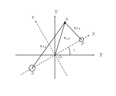
Figure 1: The inertial ($\overline{X}\overline{Y}$) and rotating ($XY$) coordinate frames are shown for the three-body problem. The center of mass of the two bodies labelled as $S$ and $P$ is the origin of both the coordinate frames and is denoted by $O$.

The units of various quantities are chosen such that the properties of the system depend only on a single parameter. Let the total mass (${\mathscr{M}}$) of the primaries ($S$ and $P$) be the unit of mass; the distance between them (${\cal D}$) be the unit of distance; and the unit of time be chosen in such a way that the angular speed of the primaries, denoted by $\Omega$, be unity. It is known that the two bodies circling around each other satisfy the following relation:

$$\Omega^{2}\;=\;\frac{G\,{\mathscr{M}}}{{\cal D}^{3}}\;,$$ (1)

where $G$ is Newton’s gravitational constant. We find it useful to express Eq. (1) in the following form:

$$\left(\frac{{\mathscr{T}}}{1\,{\rm Day}}\right)^{2}=1.33376\times 10^{5}\,\left(\frac{{\rm M}_{\odot}}{\mathscr{M}}\right)\left(\frac{{\cal D}}{1\,{\rm AU}}\right)^{3}$$ (2)

where ${\mathscr{T}}=2\pi/\Omega$ is the time-period of the binary and ${\rm M}_{\odot}$ represents the solar mass.

Figure 2: Relation between the total mass (${\mathscr{M}}$) and the time-period (${\mathscr{T}}$) of the binary. Different lines in this log-log plot correspond to different values of the binary separation (${\cal D}$).

In dimensionless units, equation (1) implies $G=1$ due to the choices made above for the units of mass, length and time; also, the mean anomaly equals time ($\tau=\overline{\tau}$ is the time as seen in both the reference frames). Figure 1 shows the binary system at an arbitrary time $\tau$ as seen in both the coordinate systems, in which $A$ is an arbitrary point, and $\mbox{\boldmath${\rm r}$}_{SA}$, $\mbox{\boldmath${\rm r}$}_{PA}$ and $\mbox{\boldmath${\rm r}$}_{OA}$ are the radius vectors of point $A$ with respect to $S$, $P$ and $O$ respectively (the axis $Z=\overline{Z}$ is not shown explicitly). Let $\xi$ be the mass of $P$, thus mass of $S$ is $(1-\xi)$. In the rotating reference frame, with positive $X$ in the direction of the body $P$, the coordinates of $P$ and $S$ will be $(1-\xi,0)$ and $(-\xi,0)$ respectively. Let $(X,Y,0)$ be the coordinate of the arbitrary point $A$, assumed to lie in the plane of the binary. Thus magnitudes of vectors $\mbox{\boldmath${\rm r}$}_{SA}$ and $\mbox{\boldmath${\rm r}$}_{PA}$ are given as:

$${\rm r}_{SA}=\lvert\mbox{\boldmath${\rm r}$}_{SA}\rvert=\sqrt{(X+\xi)^{2}+Y^{2}}$$

$${\rm r}_{PA}=\lvert\mbox{\boldmath${\rm r}$}_{PA}\rvert=\sqrt{(X-(1-\xi))^{2}+Y^{2}}$$ (3)

The gravitational potential in the comoving frame at the point $A$ may be written as,

$$\Phi\;=\;-\frac{(1-\xi)}{{\rm r}_{SA}}-\frac{\xi}{{\rm r}_{PA}}$$ (4)

2.1 Bernoulli’s principle in the rotating coordinate system

If $\mbox{\boldmath$v$}(\mbox{\boldmath$X$},\tau)$ be the fluid velocity of the wind in the rotating frame then we may write the Euler equations in rotating frame for steady flow, with $p$ and $\rho$ as the fluid pressure and density, respectively, as,

$$\left(\mbox{\boldmath$v$}\mbox{\boldmath$\cdot$}\mbox{\boldmath$\nabla$}\right)\mbox{\boldmath$v$}\,=\,-\frac{\mbox{\boldmath$\nabla$}p}{\rho}-\mbox{\boldmath$\nabla$}\Phi-\hat{\mbox{\boldmath$\Omega$}}\times\left(\hat{\mbox{\boldmath$\Omega$}}\times\mbox{\boldmath$X$}\right)-2\hat{\mbox{\boldmath$\Omega$}}\times\mbox{\boldmath$v$}$$ (5)

where $(\mbox{\boldmath$X$},\tau)\equiv(X,Y,Z,\tau)$ and $\hat{\mbox{\boldmath$\Omega$}}$ ($=\mbox{{\boldmath$\hat{e}$}}_{Z}$, which is the unit vector along $Z\equiv\overline{Z}$) is the angular velocity of the comoving frame relative to the inertial frame. Note that the equation (5) is written in dimensionless form. Using vector identities, we can write equation (5) in the following form:

$$\mbox{\boldmath$\nabla$}{\cal B}+(\mbox{\boldmath$\omega$}+2\hat{\mbox{\boldmath$\Omega$}})\times\mbox{\boldmath$v$}\;=\;{\bf 0}$$ (6)

where,

$${\cal B}\;=\;\left(\frac{1}{2}v^{2}+\int\frac{dp}{\rho}+\Phi_{\rm eff}\right)\;;\qquad\mbox{\boldmath$\omega$}\;=\;\mbox{\boldmath$\nabla$}\times\mbox{\boldmath$v$}$$ (7)

The effective potential ($\Phi_{\rm eff}$) in equation (7) is written as,

$$\Phi_{\rm eff}\;=\;\Phi-\frac{1}{2}\lvert\hat{\mbox{\boldmath$\Omega$}}\times\mbox{\boldmath$X$}\rvert^{2}\;=\;-\frac{(1-\xi)}{{\rm r}_{SA}}-\frac{\xi}{{\rm r}_{PA}}-\frac{1}{2}\lvert\hat{\mbox{\boldmath$\Omega$}}\times\mbox{\boldmath$X$}\rvert^{2}$$ (8)

On taking the dot product of equation (6) with $v$, we obtain

$$(\mbox{\boldmath$v$}\mbox{\boldmath$\cdot$}\mbox{\boldmath$\nabla$})\,{\cal B}\;=\;0$$ (9)

Therefore the quantity, ${\cal B}$, is a constant along a particular streamline for steady flows, although it could be a different constant for different streamlines. Noting the fact that the particle paths and streamlines are the same for steady flows, we can see that ${\cal B}$ remains the same for a particular fluid element as it moves along a particular streamline.

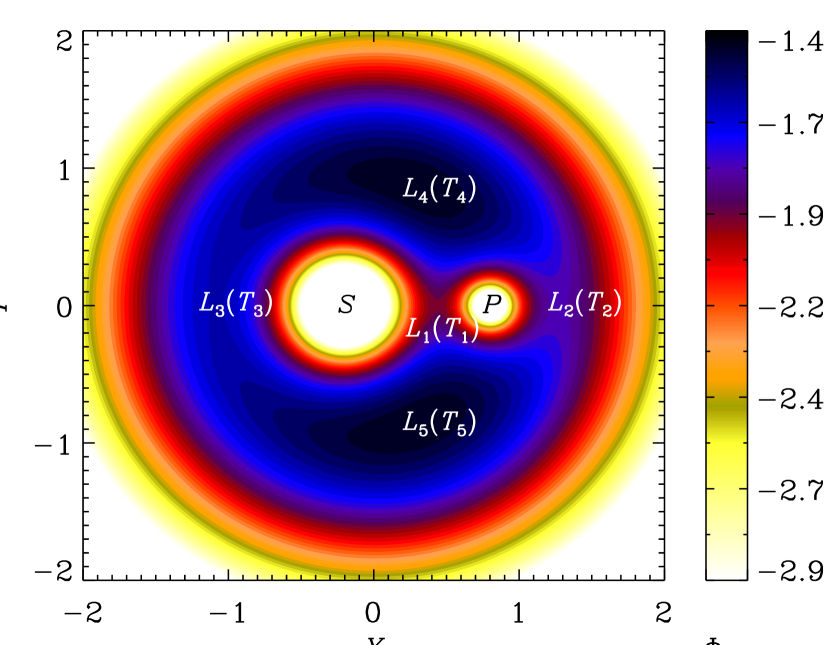
Figure 3: Isocontours of the effective potential $\Phi_{\rm eff}$ given by Eq (8), for $\xi=0.2$. Locations of Lagrangian and the temperature points are shown by $L_{1}-L_{5}$ and $T_{1}-T_{5}$, respectively.

2.2 Nature of the flow

The Lagrangian time derivative is the rate at which some quantity of interest changes as we follow any particular fluid element, which is denoted as,

$$\frac{d}{d\tau}\;=\;\frac{\partial}{\partial\tau}+(\mbox{\boldmath$v$}\mbox{\boldmath$\cdot$}\mbox{\boldmath$\nabla$})$$ (10)

As the first term on the right hand side of equation (10) (which is the Eulerian time derivative) does not contribute for steady flows, we can write from equations (9) and (10),

$$\frac{d{\cal B}}{d\tau}\;=\;(\mbox{\boldmath$v$}\mbox{\boldmath$\cdot$}\mbox{\boldmath$\nabla$})\,{\cal B}\;=\;0$$ (11)

Equation (11) implies that, for any streamline, which is same as the trajectory of a particular fluid element, we may write

$${\cal B}=\frac{1}{2}v^{2}+\left(\frac{\gamma}{\gamma-1}\right)R\,T+\Phi_{\rm eff}=\textrm{constant}=C$$ (12)

where we have used adiabatic equation of state and note that the term $\int dp/\rho$ appearing in equation (7) may be replaced by specific enthalpy ($w$) for isentropic evolution of fluid element. We know,

$$w\;=\;\left(\frac{\gamma}{\gamma-1}\right)R\,T$$ (13)

where $\gamma$ is ratio of specific heats at constant pressure and constant volume, $R$ is the gas constant and $T$ is the temperature. As the terms $v^{2}/2$ and $\{\gamma/(\gamma-1)\}\,RT$ in equation (12) cannot be negative, we infer from equation (12) that the motion of a fluid element, and hence the corresponding streamline, is restricted to the region where

$$\Phi_{\rm eff}<C$$ (14)

2.3 Isocontours of effective potential and temperature: zero velocity curves

It is known that the isocontours of the effective potential exhibit five Lagrangian points, at which the test-body may remain at rest in the comoving frame. These points are extrema or saddle points of $\Phi_{\rm eff}$. It is remarkable to note that the shape of the isocontours of the temperature distribution for binary system under consideration is identical to the isocontours of the effective potential, as may be seen from the following discussion.

Let us focus on the zero-velocity-curves, the topology of which depends on the energy of a particular fluid element. Let $\Phi_{\rm eff}=C_{1}$, where $C_{1}$ is constant. Then, we can see from equation (12) for zero-velocity-curves, that

$$\left(\frac{\gamma}{\gamma-1}\right)R\,T\, = \,C-\Phi_{\rm eff}\,=\,C-C_{1}\,=\,\textrm{constant}$$

$$\Rightarrow\quad\quad T\, = \,\textrm{constant, where,}\,\,\Phi_{\rm eff}=C_{1}\,,$$ (15)

as $\{\gamma/(\gamma-1)\}\,R$ is a constant for a particular value of $\gamma$. Thus we conclude that the shapes of the isocontours of the effective potential and the temperature are same, whereas the values might be different. Hence we will have five special temperature points, $T_{1}-T_{5}$, at the same locations where we have five special Lagrangian points, $L_{1}-L_{5}$. We may refer to these five temperature points as Lagrangian-equivalent-temperature points.

3 Direct numerical simulations

So far, we have studied the behavior of few scalar variables along streamlines. We now wish to know the trajectories of fluid elements, i.e., we would like to study how the spherically symmetric wind from the body $S$ flows in the presence of another gravitating body $P$ in a binary system. For such investigations, we use PLUTO code , which is a Godunov-type modular code intended primarily for computational astrophysics and high mach number flows in multiple spatial dimensions. The code allows us to study two-dimensional problems in a frame rotating with constant angular velocity pointing along $Z$-direction, by suitably adding noninertial (the coriolis and the centrifugal) forces in the momentum equation. The details of the code may be found in Mignone et al. (2007) (and references therein). Our strategy to study the dynamics of the wind in a binary system using PLUTO code may be expressed as follows:

1. We adapt the code in the comoving frame of the binary in which the two bodies, $S$ and $P$, appear to be at rest, by adding the necessary body-forces, namely, coriolis and centrifugal, to the equation of motion.

2. We use the hydrodynamic module of the code and solve the equations in two-dimensional $r$-$\phi$ plane, where $X=r\cos{\phi}$ and $Y=r\sin{\phi}$, and the angular velocity points in the $Z$-direction. Linearized Roe Riemann solver has been used for flux computation and we used outflow boundary conditions at the outer edge of the domain.

3. As we wish to study how the wind from one of the bodies ($S$) in binary system flows due to purely gravitational effects, we do not consider the effect of forces that might accelerate the wind radially outwards from $S$ when it leaves the surface of the body $S$ (e. g. radiation pressure on the wind due to $S$ may lead to radially outward acceleration of the wind). One may wish to imagine a radially-outward-acceleration-zone around body $S$, beyond which, the dynamics of the wind is solely governed by the gravitational effects due to binary system and the pressure gradients. The radius of such acceleration zone was chosen to be equal to $20\,\%$ of the binary separation.

4. Thus we consider the spherically symmetric wind from $S$ and study its dynamics in the plane of the binary. Equation of motion for the fluid particles is given by:

   $$\frac{\partial\mbox{\boldmath$v$}}{\partial\tau}\,+\,\left(\mbox{\boldmath$v$}\mbox{\boldmath$\cdot$}\mbox{\boldmath$\nabla$}\right)\mbox{\boldmath$v$}\,=\,-\frac{\mbox{\boldmath$\nabla$}p}{\rho}-\mbox{\boldmath$\nabla$}\Phi_{\rm eff}-2\hat{\mbox{\boldmath$\Omega$}}\times\mbox{\boldmath$v$}$$ (16)

   where symbols have ususal meanings described earlier. As our aim is to illustrate the physical mechanism, we are not much interested in absolute values of various physical quantities, but their relative changes as one moves about in space at any given time, would indeed be useful for our further modelling.

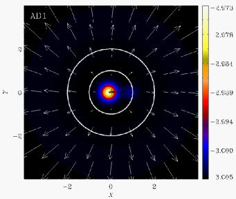
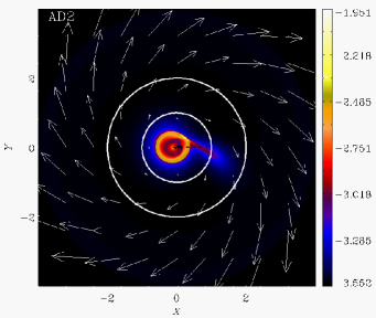
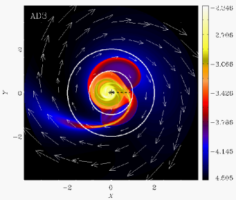
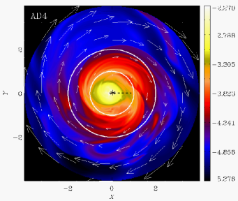
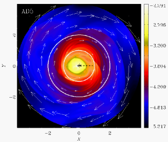
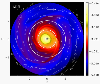
Figure 4: ($\xi=0.1$) Snap-shots of logarithmic density maps, as seen from the corotating frame; colours indicate $\log_{10}\rho$. Time increases from upper-left to lower-right panel. Two concentric circles are centered about the common center of mass of the binary, denoted by the asterisk (‘$\ast$’). The dashed line joins the centers of the two components of the binary, where the star, $S$ (with the wind), lies at the left end, whereas the other body, $P$, lies at the right end. Arrows indicate the velocity vector field.

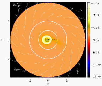
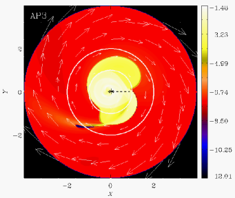
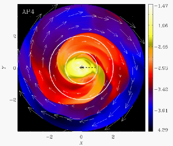
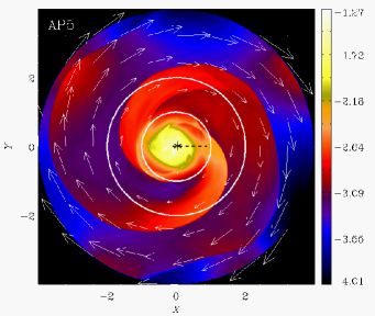
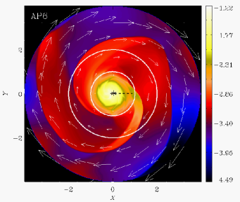
Figure 5: Similar to Fig. (4) but shows the snap shots of the pressure maps on logarithmic scale ($\log_{10}P$).

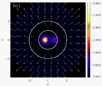
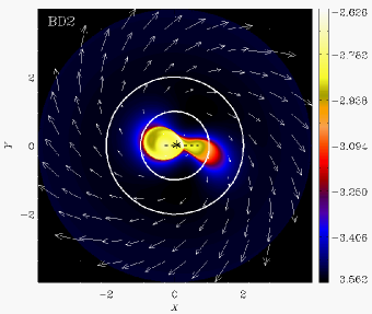
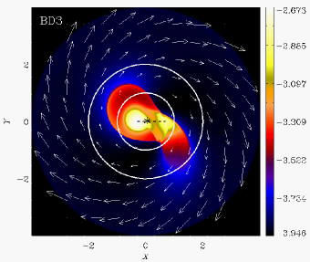
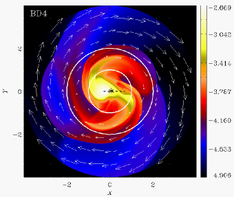
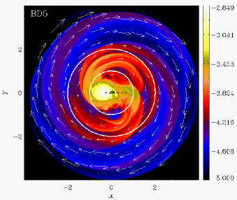
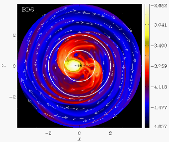
Figure 6: Same as Fig. (4) but for $\xi=0.3$.

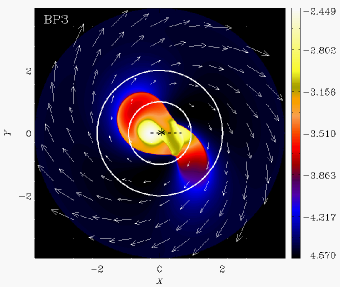
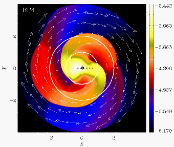
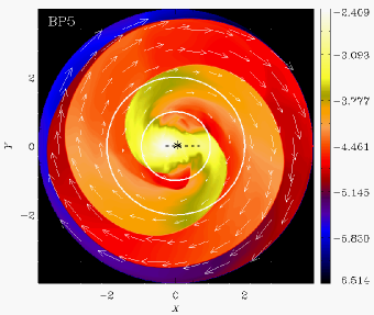
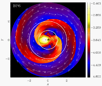
Figure 7: Same as Fig. (5) but for $\xi=0.3$.

3.1 Spiral nature of outflowing gas

We present results from two different simulations with $\xi=0.1$ (model A) and $0.3$ (model B), and show the evolution of density/pressure maps with time as seen in the corotating frame, which is the rest frame of the binary system. The domain in $r$- and $\phi$- extends from $0$ to $4$ and $0$ to $2\pi$, respectively, with ${\cal D}$ being the distance unit. The grid resolutions were chosen to be $300\times 300$ for model A and $400\times 400$ for model B, in $r\times\phi$ domain. We reduced the total mass (${\mathscr{M}}$) of the binary by factor $4$ in simulation with $\xi=0.3$ as compared to the one with $\xi=0.1$. As noted before, ${\mathscr{M}}$ is the unit of mass in this work.

In Figs (4) and (5) we show, respectively, the snapshots of the density and pressure, both in logarithmic units ($\log_{10}\rho$ and $\log_{10}P$), for the model with $\xi=0.1$. Time increases from panel AD1 (AP1) to AD6 (AP6) and we see the development of the spiral pattern of the outflowing material. The evolution reaches a steady state in later stages and thus we find that the structure of the velocity field stops to evolve considerably. We note that the symmetry axis of the spiral pattern is shifted from the rotation axis (which passes through the center of mass of the binary) by distance $\xi$. The whole pattern of density/pressure as shown in Fig (4)/(5) rotates with binary period for an inertial observer, and thus we find periodic variation in the mass density along a given sightline. To illustrate this, we have drawn two concentric circles, centered around the common center of mass of the binary, showing the density/pressure variations as one goes around the circles. The period of such density modulations will be of the order of binary period.

Similarly we show snapshots of density and pressure for the model with $\xi=0.3$ in Figs (6) and (7), respectively. As before we find that the stellar wind spirals outward and reaches a steady state. The structure of the velocity field stays nearly the same in late stages, which would be crucial to explain the observational fact that the maser spot does not move in the sky. Although our aim is to propose a physical model which can explain some key qualitative features seen in the observations related to maser intensity variations, we find that a closer look of Figs (4)–(7) reveals that the density at some spatial location along a particular sightline might vary easily by a factor of about $10$ between its maximum and minimum values.

To make contact with physical units, we refer the reader to Fig. (2) where we show the relation between the total mass (${\mathscr{M}}$) and the time-period (${\mathscr{T}}$) of the binary, corresponding to different values of the binary separation (${\cal D}$); see also Eq. (2). The mass, period and distance are expressed in terms of solar mass, day and astronomical unit (AU), respectively. If we let the distance unit in our simulations to be equal to $1\,{\rm AU}$, the periods corresponding to total masses equal to $1\,{\rm M}_{\odot}$ and $50\,{\rm M}_{\odot}$ will be about $1\,{\rm year}$ and $50\,{\rm days}$, respectively.

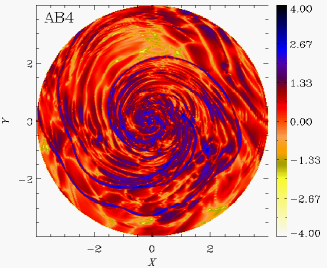
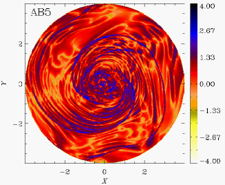
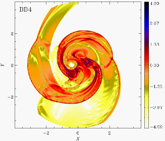
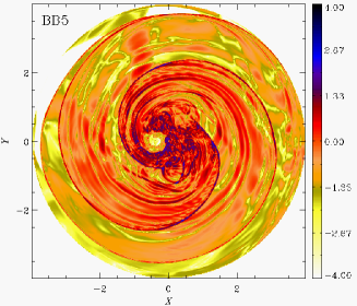
Figure 8: Snapshots of the quantity, $\log_{10}|\mbox{\boldmath$\beta$}|$ (shown by colours; $|\mbox{\boldmath$\beta$}|\equiv|\beta_{Z}|$ in this setup), for models A (top panels; $\xi=0.1$) and B (bottom panels; $\xi=0.3$). Left and right panels correspond to panels $4$ and $5$ of Figs. (4)-(7).

3.2 Baroclinicity

We now turn to a completely different phenomena which will have implications for the generation of the vorticity, given by $\mbox{\boldmath$\omega$}=\mbox{\boldmath$\nabla$}\mbox{\boldmath$\times$}\mbox{\boldmath$v$}$. Given that the flow around binaries in star-forming regions are expected to be highly ionized, this is usually studied under standard magnetohydrodynamics (MHD). Although the study of magnetic fields and the plasmas is beyond the scope of the present paper, we, however, wish to remark that the magnetic field, $B$, could also evolve due to the presence of baroclinicity, in the same model setup. The mathematical form of the evolution equations of the vorticity and the magnetic field are same; these may be expressed as,

$$\frac{\partial\mbox{\boldmath$B$}}{\partial t} = \mbox{\boldmath$\nabla$}\mbox{\boldmath$\times$}(\mbox{\boldmath$v$}\mbox{\boldmath$\times$}\mbox{\boldmath$B$})+\frac{\mbox{\boldmath$\nabla$}P\mbox{\boldmath$\times$}\mbox{\boldmath$\nabla$}\rho_{p}}{\rho_{p}^{2}}+\eta\nabla^{2}\mbox{\boldmath$B$}$$ (17)

$$\frac{\partial\mbox{\boldmath$\omega$}}{\partial t} = \mbox{\boldmath$\nabla$}\mbox{\boldmath$\times$}(\mbox{\boldmath$v$}\mbox{\boldmath$\times$}\mbox{\boldmath$\omega$})-\frac{\mbox{\boldmath$\nabla$}P\mbox{\boldmath$\times$}\mbox{\boldmath$\nabla$}\rho}{\rho^{2}}+\nu\nabla^{2}\mbox{\boldmath$\omega$}$$ (18)

where $\eta$, $\nu$ and $\rho_{p}$ are the magnetic diffusivity, the kinematic viscosity and the plasma density, respectively. The second term on the right hand side of Eq (17) (or 18) is known as the baroclinic term, which can lead to the generation of $B$ (or $\omega$) even if the magnetic field (or vorticity) was strictly zero to begin with. The baroclinicity characterizing the misalignment between the isocontours of the pressure and the density may be expressed as,

$$\mbox{\boldmath$\beta$}\,=\,\frac{\mbox{\boldmath$\nabla$}P\mbox{\boldmath$\times$}\mbox{\boldmath$\nabla$}\rho}{\rho^{2}}$$ (19)

In the same model being discussed here, the baroclinic vector field $\beta$ is zero everywhere initially. It is instructive to see if such a field could be generated at later stages of evolving stellar wind in the Roche potential. To study this we considered both the models A and B, discussed above, for which we have two dimensional data (in the plane of the binary) of the density and the pressure fields at different instances of times; few snapshots of density and pressure are shown in Figs (4)–(7). From this data, we compute $\beta$ using Eq (19) which points along $\pm\mbox{{\boldmath$\hat{e}$}}_{Z}$ by definition, as both the vector fields, $\mbox{\boldmath$\nabla$}P$ and $\mbox{\boldmath$\nabla$}\rho$, lie in the plane of the binary in our 2D setup. We find that $\beta$ changes sign in the binary plane, but its magnitude is quite large, especially along the spirals. In Fig. (8) we show the snapshots of the quantity $\log_{10}|\mbox{\boldmath$\beta$}|$ for models A (top panels) and B (bottom panels), in the late stages of the simulations.

Thus in the same setup, we show that the baroclinicity develops significantly, which can source the vorticity field and also the magnetic field if the fluid is electrically conducting, according to Eqs. (17) and (18). Similar conditions are expected to exist in many parts of a galaxy, and therefore this provides yet another possibility by which the seed magnetic fields could arise within the galaxy. The spatial scales of variations of $\beta$ are smaller compared to the binary orbit and therefore this could source the seed magnetic (or vorticity) fields at small scales. Detailed investigations focussing on the magnetic fields, giving quantitative estimates, are needed, and will be studied in a future work.

4 Maser variability (light-curve)

Now we focus on the possible distribution of maser sources in the medium around the binary system, as seen by the observer in the defined geometry. The apparent (line-of-sight) velocity structure and the column density of the molecular matter (for relevant species) are amongst the key ingredients governing the formation of astronomical masers. Hydrodynamic simulations presented in § 3 reveal the flow structure and distribution of column density in our model setup. We make use of these essential informations and perform further numerical simulations to study the masing action in such environment. For simplicity, we have used a single-arm spiral pattern in these simulations, instead of a two-arm spiral structure as suggested from PLUTO simulations presented in the previous section. We note that the patterns of field variables (mass density, pressure and baroclinicity), shown in Figs (4)–(8), rotate with the angular speed ($\Omega$) of the binary, for an observer in a fixed inertial frame. In this section we present our results as would be seen by an inertial observer.

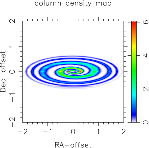
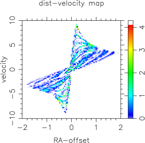
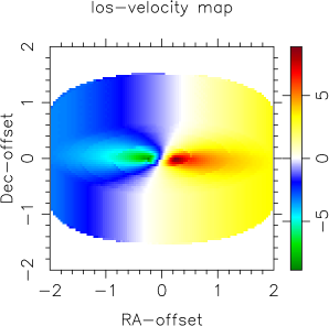
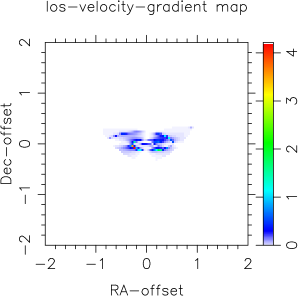
Figure 9: Maps of (i) column density (top left); (ii) distance-velocity (top right; colours: maser intensity); (iii) component of velocity along the line of sight (bottom left); and (iv) the gradient of velocity along sightline (bottom right), in a fixed inertial frame, shown for a binary system with angle of inclination $i_{\rm A}=60^{\circ}$. Colors indicate the corresponding quantities on arbitrary scale.

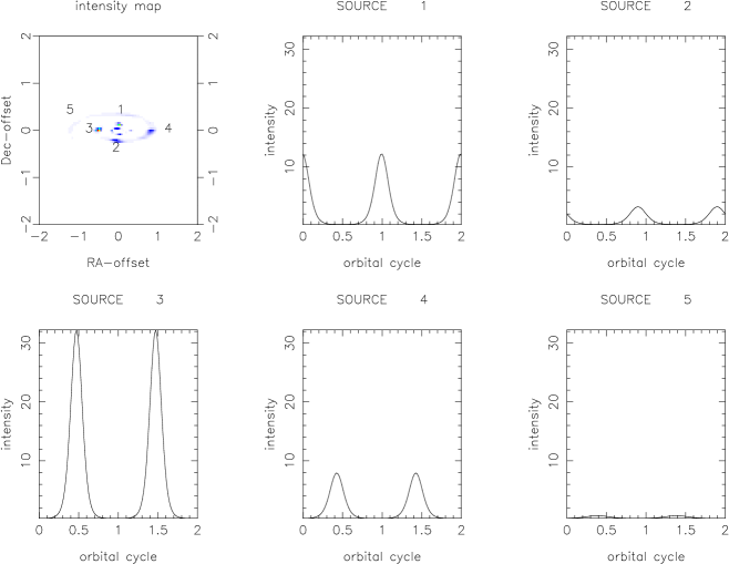
Figure 10: Maser intensity map around a binary system with an inclination angle $i_{\rm A}=60^{\circ}$ shown in top left panel, where locations of five masing spots are marked; seen from a fixed inertial frame. Lightcurves of all these five sources are shown in the rest of the panels.

Physical mechanisms governing the laws of maser formation in cosmic settings are complex and have been studied extensively (see e.g. Goldreich & Keeley (1972); Strel’nitskiĭ (1974); Elitzur (1992)). A widely accepted model for class II methanol masers is by Sobolev & Deguchi (1994). Here our focus is on the conditions which can potentially cause periodic variations in maser intensities, while also being able to address the observational fact that the sky locations of the maser spots stay fixed with time. We do not intend to study the formation mechanisms of maser and refer the reader to earlier works, some of them quoted above, for further related studies. For our purposes, it is sufficient to note that the intensity of maser, ${\cal I}\propto\exp{(-\tau)}$, where $\tau$ is optical depth (negative for amplification), which varies along a particular sightline, and can be expressed in an average sense as,

$$\tau\,\propto\,\frac{\Sigma}{\Delta v_{\parallel}}\,,$$ (20)

where $\Sigma$ is the mass column density of the medium and $\Delta v_{\parallel}$ is the velocity spread along the chosen line of sight. Thus the sightlines with vanishing velocity gradients are ideal for masing action. If the structure of the velocity field in the sky does not change, then the masing spot is expected to stay at the same sky location.

Let ${\cal R}$ denote the location of the masing spot in the sky, seen from the fixed coordinate frame $\overline{X}\,\overline{Y}\,\overline{Z}$. If the density of the medium at ${\cal R}$ varies sinusoidally in time as, $\rho(\mbox{\boldmath${\cal R}$},t)\sim\rho_{0}\sin{(\omega t+\varphi)}+\rho_{\rm f}$, then, to lowest order in $\tau$, the maser intensity will also show sinusoidal temporal modulation with the same period ($=2\pi/\omega$), as may be seen from Eq (20). Thus any temporal modulation in the column density will result in maser intensity variation. The quantities $\rho_{0}$, $\omega$, $\varphi$ and $\rho_{\rm f}$ denote, respectively, the amplitude, angular frequency of modulation, the phase and the floor density. Given that the density maps shown in § 3 rotate with angular speed ($\Omega$) of the binary, for an inertial observer along a chosen line of sight, the observed density at ${\cal R}$ will show modulations with the angular frequency ($\omega$) which is comparable to $\Omega$, i.e., $\omega\sim{\cal O}(\Omega)$. As we have modelled a single-arm spiral structure, for simplicity, in this section (instead of two-arm spiral structure suggested from PLUTO simulations), we note that the orbital periods will be overestimated by factor two. We emphasize again that our aim here is to explore possible physical conditions that can lead to observed periodic modulations in maser intensities. One of the conclusions from our study may be stated as: the binary period determines the period of maser intensity variations.

Binary orbits might be inclined at arbitrary angles with respect to sightlines. The inclination angle ($i_{\rm A}$) may be defined as the angle between normal to the binary plane and outwardly pointed line of sight. We wish to illustrate the emission patterns when the binary lies somewhere between the edge-on ($i_{\rm A}=90^{\circ}$) and the face-on ($i_{\rm A}=0^{\circ}$) configurations. Here we consider a binary with $i_{\rm A}=60^{\circ}$. We identify maser emitting regions in our simulations and study the temporal evolutions of the maser intensities from many different sources.

Figure (9) shows maps of various physical quantities of interest at some time and we briefly discuss these below:

1. The column density shows single-arm spiral structure where the density decreases as we move away from the central regions; top left panel.

2. Remarkably, the distance-velocity diagram in top right panel shows clearly the bipolar structure, as has been widely observed. This is a natural outcome of our studies which suggests that the observed bipolar nature of molecular outflows could also arise due to presence of binary systems.

3. Bottom left panel shows the map of the component of velocity along the line of sight. It is useful to note that the structure of the velocity field remains the same with time in this setup and therefore the potential maser spots do not move in the sky, thus explaining this observational fact.

4. The map of velocity gradient along the line of sight is shown in bottom right panel. Low gradients in velocity determine the potential sites where the masing action can take place, as may be seen from Eq (20).

This leads us to construct and monitor maser intensity maps as functions of time. In Fig. (10) we show a typical map of maser intensity at some time (top left panel), where we mark the locations of five different sources (masing spots). We intend to show the variations of maser intensities as functions of time, or equivalently, as functions of orbital cycle of the binary. Such plots of intensity variation, commonly called light-curves, corresponding to all five sources are shown in other panels of Fig. (10). Some noteworthy properties are as follows:

1. We first notice that the maser intensities show periodic temporal modulations. These modulations are caused by the periodic variation of column density, as discussed above, and the period is determined by the binary period.

2. Multiple masing spots could form around a single binary system, and all these sources have same periods of modulation, as they arise due to density variations, the period of which, in turn, is determined by the binary system. However, the amplitudes of intensity variations are different for different sources.

3. Thus we argue that the observed periods of such intensity variations trace the characteristics of the binary, i.e., the binary period. This, together with some other independent estimates of either the mass or separation of the binary, could be very useful in determining the nature of binary systems, embedded in molecular clouds.

4. Both, the arc-like and somewhat symmetric spots, are possible; compare, e.g., spots ‘2’ and ‘3’ in Fig. (10). This might depend on the local physical conditions and the distances of the spots from central regions. Linear structures could indeed be reminiscent of Keplerian-like velocity gradient, as has been conjectured by Norris et al. (1998).

5 Conclusions

With an aim to provide physical mechanisms that could potentially cause observed periodic variations in the maser intensities, we studied the dynamics of stellar wind from one of the bodies in the binary system. We find that the intensity variations are due to the periodic variations in the local material density, where the period is on the order of the binary period. The underlying velocity structure is Keplerian-like and it remains frozen-in-time in the later stages. We note that this non-evolving velocity structure is important for the masing spots to stay at the same sky location, as has been revealed by the observations, and it is the maser intensity which varies periodically. The wind appears to spiral outwards before settling into the faraway Keplerian orbits, and naturally appears bipolar in the standard position-velocity diagram.

The spherical symmetry of the stellar wind is broken due to the influence of the other gravitating body. This symmetry breaking very near to the star in the binary system holds the key to establishing density inhomogenieties also far away from the binary location where the conditions for masing action are favourable. We first studied this probelm in the rotating frame in which the binary components are at rest. To an inertial observer, such density inhomogeneities in the rotating frame lead to a periodic density variations along a chosen line of sight. Sightlines with nearly vanishing velocity gradients along those directions being ideal for observing masers show sinusoidal modulation in the material density, thus causing the maser intensity also to show sinusoidal variation. The structure of the velocity field being nearly frozen, which is close to Keplerian, explains why these periodically varying maser spots do not move. This mechanism also naturally gives a bipolar appearance in the standard position-velocity diagram. We note that the bipolar outflows are ubiquitously observed in nature and are presumably thought to be associated with star forming regions in molecular clouds. A binary origin may be responsible for some of these bipolar outflows.

In the same setup, we also find that the baroclinicity develops and it is mostly concentrated in the spiral form; see Fig. (8). This offers yet another scenario, which can lead to the generation of seed vorticity and magnetic fields within the galaxies, and might further affect the evolution of these fields. More detailed investigations focussing primarily on the magnetic fields will be presented in a future work.

References

- Araya et al. (2010) Araya, E. D., Hofner, P., Goss, W. M., Kurtz, S., Richards, A. M. S., Linz, H., Olmi, L. & Sewilo, M., 2010, ApJL, 717, L133
- Bachiller et al. (1996) Bachiller, R., 1996, ARA&A, 34, 115
- Brandenburg & Subramanian (2005) Brandenburg, A. & Subramanian, K., 2005, Physics Reports, 417, 1-209
- Canto et al. (1981) Canto, J., Rodriguez, L. F., Barral, J. F. & Carral, P., 1981, ApJ, 244, 102
- Díaz-Jiménez & French (1988) Díaz-Jiménez, A. & French, A. P., 1988, Am. J. Phys., 56, 85
- Ellingsen (2006) Ellingsen, S. P., 2006, ApJ, 638, 241
- Elitzur (1992) Elitzur, M., Astronomical Masers, Springer-Science (1992)
- Goedhart, Gaylard & van der Walt (2004) Goedhart, S., Gaylard, M. J. & van der Walt, D. J., 2004, MNRAS, 355, 553
- Goedhart et al. (2005) Goedhart, S., Minier, V., Gaylard, M. J. & van der Walt, D. J., 2005, MNRAS, 356, 839
- Goedhart et al. (2009) Goedhart, S., Langa, M. C., Gaylard, M. J. & van der Walt, D. J., 2009, MNRAS, 398, 995
- Goldreich & Keeley (1972) Goldreich, P. & Keeley, D. A., 1972, ApJ, 174, 517
- Harmon, Leidel & Lindner (2003) Harmon, N. J., Leidel, C. & Lindner, J. F., 2003, Am. J. Phys., 71, 871
- Hendel (1983) Hendel, A. Z., 1983, Am. J. Phys., 53, 746
- Hendel & Longo (1988) Hendel, A. Z. & Longo, M. J., 1988, Am. J. Phys., 56, 82
- Heyer et al. (1986) Heyer, M. H. et al, 1986, ApJ, 308, 134
- Königl (1982) Königl, A., 1982, ApJ, 261, 115
- Lada (1985) Lada, C. J., 1985, ARA&A, 23, 267
- Menon & Agrawal (1986) Menon, V. J. & Agrawal, D. C., 1986, Am. J. Phys., 54, 752
- Mignone et al. (2007) Mignone, A., Bodo, G., Massaglia, S., Matsakos, T., Tesileanu, O., Zanni, C., & Ferrari, A., 2007, ApJS, 170, 228
- Minier, Booth & Conway (2002) Minier, V., Booth, R. S. & Conway, J. E., 2002, A&A, 383, 614
- Modestov et al. (2014) Modestov, M., Bychkov, V., Brodin, G., Marklund, M. & Brandenburg, A., 2014, eprint arXiv:1402.2761
- Morin (2008) Morin, D., Introduction to classical mechanics, Cambridge University Press, Cambridge (2008)
- Norris et al. (1998) Norris, R. P. et al., 1998, ApJ, 508, 275
- Poincaré (1890) Poincaré, H., 1890, Acta Math., 13, 1-270
- Shu et al. (1987) Shu, F. H., Adams, F. C. & Lizano, S., 1987, ARA&A, 25, 23
- Shu et al. (1991) Shu, F. H., Ruden, S. P., Lada, C. J. & Lizano, S., 1991, ApJ, 370, L31
- Snell (1983) Snell, R. L., 1983, RMAA, 7, 79
- Snell et al. (1980) Snell, R. L., Loren, R. B. & Plambeck, R. L., 1980, ApJ, 239, L17
- Sobolev & Deguchi (1994) Sobolev, A. M. & Deguchi, S., 1994, A&A, 291, 569
- Strel’nitskiĭ (1974) Strel’nitskiĭ, V. S., 1974, Usp. Fiz. Nauk, 113, 463
- Subramanian (2008) Subramanian, K., 2008, arXiv:0802.2804
- Szymczak et al. (2011) Szymczak, M., Wolak, P., Bartkiewicz, A. & van Langevelde, H. J., 2011, A&A, 531, L3
- Torrelles et al. (1983) Torrelles, J. M. et al, 1983, ApJ, 274, 214
- Valtonen & Karttunen (2005) Valtonen, M. & Karttunen, H., The three-body problem, Cambridge University Press, Cambridge (2005)
- van der Walt, Goedhart & Gaylard (2009) van der Walt, D. J., Goedhart, S. & Gaylard, M. J., 2009, MNRAS, 398, 961
- Walsh et al. (1998) Walsh, A. J., Burton, M. G., Hyland, A. R. & Robinson, G., 1998, MNRAS, 301, 640
- Welch et al. (1985) Welch, W. J., Vogel, S. N., Plambeck, R. L., Wright, M. C. H. & Bieging, J. H., 1985, Science, 228, 1329