FUV variability of HD 189733. Is the star accreting material from its hot Jupiter?

Abstract

Hot Jupiters are subject to strong irradiation from the host stars and, as a consequence, they do evaporate. They can also interact with the parent stars by means of tides and magnetic fields. Both phenomena have strong implications for the evolution of these systems. Here we present time resolved spectroscopy of HD 189733 observed with the Cosmic Origin Spectrograph (COS) on board to HST. The star has been observed during five consecutive HST orbits, starting at a secondary transit of the planet ($\phi\sim 0.50-0.63$). Two main episodes of variability of ion lines of Si, C, N and O are detected, with an increase of line fluxes. Si IV lines show the highest degree of variability. The FUV variability is a signature of enhanced activity in phase with the planet motion, occurring after the planet egress, as already observed three times in X-rays. With the support of MHD simulations, we propose the following interpretation: a stream of gas evaporating from the planet is actively and almost steadily accreting onto the stellar surface, impacting at $70-90\deg$ ahead of the sub-planetary point.

1 Introduction

The significant fraction ($\sim 10\%$) of known exoplanets with masses of the order of the Jupiter mass and orbiting within few stellar radii (hot Jupiters) raised the question of their origin and evolution. Because of their proximity to the parent star, these planets are strongly irradiated, their upper atmospheres are bloated and do evaporate (Vidal-Madjar et al., 2003; Lecavelier des Etangs et al., 2004; Lecavelier Des Etangs et al., 2010; Linsky et al., 2010; Ben-Jaffel & Ballester, 2013). It is plausible that the evaporating material forms a cometary tail and some sort of bow shock in front of the planet due to the interaction with the stellar wind (Cohen et al., 2011; Ben-Jaffel & Ballester, 2013; Llama et al., 2013).

Furthermore, interactions of tidal and magnetic nature are likely to occur in systems with hot Jupiters (Cuntz et al., 2000; Saar et al., 2004; Lanza, 2009; Lanza et al., 2010, 2011; Cohen et al., 2009, 2010, 2011). Stars can receive angular momentum from their hot Jupiters during the migration and circularization of the planet’s orbit. The external input of angular momentum to the star reduces its decline with age during the main sequence due to wind losses. Because of the connection between stellar activity, age and rotation, the stellar activity of the stars can be effectively boosted in presence of hot Jupiters, mimicking a younger age as demonstrated for the systems of HD 189733 and Corot-2A (Pillitteri et al., 2010, 2011; Schröter et al., 2011; Pillitteri et al., 2014a; Poppenhaeger & Wolk, 2014). Tides can be produced on the stellar surface, with height proportional to $d^{-3}$ so the closer is the planet the stronger is the effect, that occurs twice per orbital period. However, in extreme cases, e.g. WASP-18 (Pillitteri et al., 2014b), the influence of the tidal perturbation could destroy the magnetic dynamo of stars with shallow convective zones. It is also suggested that the strong tidal stresses in WASP-18 reduce significantly the mixing inside the convective zone, as evidenced by a high Li abundance. This is at odds with the finding that planet host stars have depleted more Li than single stars (Delgado Mena et al., 2014; Bouvier, 2008; Gonzalez, 2008; Israelian et al., 2004).

Magnetospheric interactions between planetary and stellar magnetic fields can be the source of additional reconnection events, and perturbations of the magnetic field topology. As a result, more flares could manifest in systems with hot Jupiters than in single stars of the same age. Furthermore, the planetary magnetic field can efficiently trap the stellar wind and its angular momentum, modifying the losses of rotation and keeping the star rotating faster than expected for its age (Cohen et al., 2011).

Shkolnik et al. (2003, 2005, 2008); Walker et al. (2008) reported evidences of chromospheric activity phased with the planetary orbital motion in the systems of $\mu$ And, HD 179949 and HD 189733, probed by Ca H&K lines. Interestingly, all cases exhibit a phase shift: the site of enhanced activity on the stellar surface is $70-80\deg$ in the case of HD 179949 and $169\deg$ for $\mu$ And leading the sub-planetary point.

In X-rays, we observed enhanced flare variability in HD 189733 after the eclipse of the planet ($\phi=0.5$) in a restricted range of phases $\phi=0.52-0.65$ (Pillitteri et al., 2010, 2011, 2014a). The rate of such flare activity in HD 189733 is higher than in stars a few Gyr old, and similar to that of pre-Main Sequence stars or stars more active than the Sun. Furthermore, this type of variability has not been observed at the planetary transits, rising the question whether HD 189733 has a prevalent X-ray activity at some orbital phases of its hot Jupiter (Pillitteri et al., 2011, 2014a). An active spot on the stellar surface, at $\sim 70-90\deg$ ahead of the sub-planetary point, magnetically connected with the planet, and co-moving with the planet had been hypothesized (Pillitteri et al., 2014a). Such spot would emerge at the edge of the stellar disk when the planet is in a range of phases of $\phi=0.52-0.65$, originating thus a phased variability.

Lanza et al. (2010) explains this phenomenon with an analytical model of the stellar field. The main hypothesis is that a magnetic link between the star and the planet exists if the planet is sufficiently close to the star as in case of hot Jupiters. The lines of the magnetic field of the star could connect with the dipolar field of the planet via a bent path and generate thus the phase lag. The relative motion of the planet with respect to the star plays a key ingredient for generating such configuration. In Lanza (2012) this model is further refined, with the planet motion inducing reconnection events near the surface of the star.

Cohen et al. (2011) modeled the magnetic SPI in HD 189733 including a more realistic stellar magnetic field. Their magneto-hydrodynamic (MHD) simulations show that at certain phases the planet can induce reconnection events and flares if the planet encounter locally enhanced stellar magnetic field. The same model predicts the rate of exoplanet atmosphere loss, and the cometary tail that the planet motion is winding around its orbit. Preusse et al. (2006) and Kopp et al. (2011) modeled the interaction between planet and star by means of alfvènic waves hitting the surface of the star, generated by the planet acting as a conductor moving within the stellar magnetic field and the stellar wind. This model can reproduce well the observed phase lag of chromospheric activity which arises from the relative motion of the planet and the star.

Among the systems with hot Jupiters, HD 189733 is a privileged target where to study SPI effects, planet evaporation and the dynamics of the planetary gas around the host star. It is composed of a K1.5V type star as primary component ($P_{\rm rot}=11.9$ d, $d=19.3$ pc from the Sun), and an M4 companion, HD 189733 B, at 3200 AU from the primary. HD 189733 A hosts a hot Jupiter class planet (HD 189733b) at a distance of only 0.031 AU (about 8.5 stellar radii) with an orbital period of $\sim 2.22$d (Bouchy et al., 2005).

In this paper we present observations of HD 189733 obtained with the Cosmic Origin Spectrograph (COS) on board HST. The aim of our observations is to obtain time resolved spectroscopy of HD 189733 at the post planetary eclipse phases, as observed with XMM-Newton, in order to find signatures of SPI in FUV and to better recognize and understand any phased activity in HD 189733. Previous observations in FUV of HD 189733 with HST COS and STIS have focused at the planetary transits. These observation revealed the evaporation of the planetary atmosphere and an estimate of the mass loss (Lecavelier Des Etangs et al., 2010), and asymmetry of ingress and egress implying a bow shock in front of the planet due to the interaction between the stellar wind and the planetary escaping atmosphere (Lecavelier des Etangs et al., 2012; Bourrier et al., 2013; Ben-Jaffel & Ballester, 2013; Llama et al., 2013). Motivated by our findings in X-rays, we argue that observing HD 189733 at the planetary eclipse in FUV can offer new insights on the dynamics of the gas evaporating from the planet and of the structure of the chromosphere and transition region of the star. The paper is structured as follows: in Sect. 2 we describe the observations and the data analysis; Sect. 3 details the results, in Sect. 4 we discuss the results, and in Sect. 5 we present our conclusions.

2 Observations and data analysis

We observed HD 189733 with HST and COS spectrograph on September 12 2013. The observations were carried along five consecutive HST orbits, spanning the planetary orbital phases of 0.4996 through 0.6258 (see Table 1 and Fig. 1, left panel). We used the grating G130M with central wavelength of 1300Å that encompasses the range 1150Å to 1450Å and has a gap between the two detector segments in the range $\sim 1294-1309$ Å. The effective area of COS paired with grating G130M is above 1500 cm² with a peak of 2500 cm² around 1220Å. For the transit and period, we used the ephemeris from Triaud et al. (2009), which are based on the analysis of optical spectra obtained with the HARPS spectrograph at the ESO 3.6 m telescope in La Silla (Chile). When using the ephemeris from Agol et al. (2010), based on Spitzer observations, this would result in a systematic shift of $\sim-249.1$ s with respect to the optical ephemeris of Triaud et al. (2009).

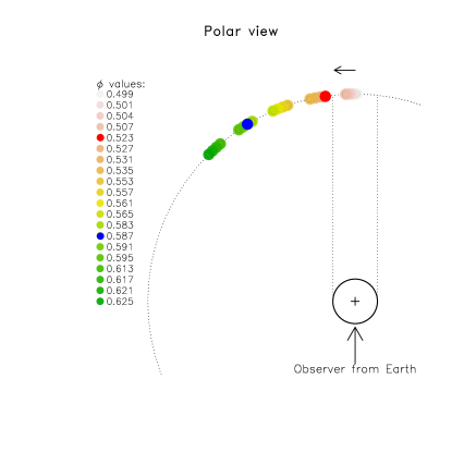
Figure 1: Left panel: schematic of the planetary phases during the COS exposures. Right panel: average spectrum obtained from the five HST orbits and the sum of the COS exposures. We marked the main ion lines in the two wavelength ranges. A detailed plot of the spectrum is available at www.astropa.inaf.it/~pilli/hd189733_hst_cos.pdf.

The average spectrum from the five orbits is shown in Fig. 1, right panel. The total exposure is about 12.1 ks. The main lines in this range are HI Ly$\alpha$, Si II, Si III, and Si IV lines, C II and C III lines, and N V lines. A list of these lines, with the peak of formation temperature, line intensity, and spectroscopic terms is given in Table 2. These data are taken from Chianti database (Dere et al., 1997; Landi et al., 2013). However, other small lines are visible in our spectra and missing from Chianti. For identifying these lines we used NIST database (Kramida et al., 2014). To help the identification of the lines, we produced an atlas of the spectrum, plotted in pieces of 10Å. In each panel lines from Chianti are labelled, tickmarks at the NIST wavelengths of line of different elements (only those with relative accuracy $\leq 50\%$) are indicated with different colors. Most of these lines are from Fe ions, Al, Si, and S. Also, airglow lines are marked with light blue bands across the spectrum. Fig. 2 shows a close up plot of selected line profiles for three spectra: average spectrum of first orbit, and exposures nr. 5 and nr. 14, that show two episodes of flux increases in several lines.

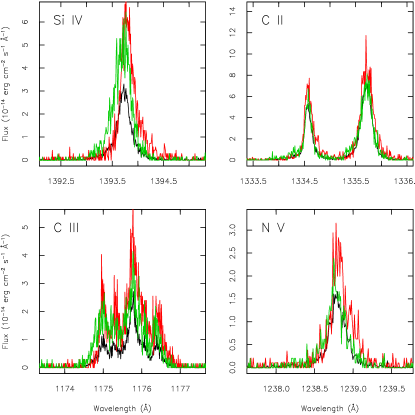
Figure 2: Examples of line profiles in three spectra: average of first orbit (black), exposure nr. 5 (red), and exposure nr. 14 (green). The names of the ions are indicated in the panels. The lines show an increase of flux and centroid shifts at these two exposures.

Table 1: Log of the HST observations.

Orbit	Nr.	Exposure id.	Date	JD (days)	Planetary phase∗	Exposure (s)
I	1	lc0u01qjq	2013:09:12T10:14:21	2456547.92663194	0.4996	431.0
	2	lc0u01qlq	2013:09:12T10:23:27	2456547.93295139	0.5025	440.0
	3	lc0u01qnq	2013:09:12T10:32:42	2456547.93937500	0.5054	440.0
	4	lc0u01qpq	2013:09:12T10:41:57	2456547.94579861	0.5083	440.0
II	5	lc0u01qrq	2013:09:12T11:31:45	2456547.98038194	0.5239	640.2
	6	lc0u01qtq	2013:09:12T11:44:20	2456547.98912037	0.5278	652.2
	7	lc0u01qvq	2013:09:12T11:57:16	2456547.99810185	0.5318	654.2
	8	lc0u01qxq	2013:09:12T12:10:14	2456548.00710648	0.5359	649.2
III	9	lc0u01qzq	2013:09:12T13:07:25	2456548.04681713	0.5538	648.2
	10	lc0u01r1q	2013:09:12T13:20:17	2456548.05575231	0.5578	646.2
	11	lc0u01r3q	2013:09:12T13:33:70	2456548.06466435	0.5618	646.2
	12	lc0u01r5q	2013:09:12T13:45:57	2456548.07357639	0.5659	646.2
IV	13	lc0u01r7q	2013:09:12T14:43:70	2456548.11327546	0.5838	648.2
	14	lc0u01r9q	2013:09:12T14:55:59	2456548.12221065	0.5878	646.2
	15	lc0u01rbq	2013:09:12T15:08:49	2456548.13112269	0.5918	646.2
	16	lc0u01rdq	2013:09:12T15:21:39	2456548.14003472	0.5958	646.2
V	17	lc0u01rfq	2013:09:12T16:18:50	2456548.17974537	0.6137	648.2
	18	lc0u01rhq	2013:09:12T16:31:42	2456548.18868056	0.6177	646.2
	19	lc0u01rjq	2013:09:12T16:44:32	2456548.19759259	0.6218	646.2
	20	lc0u01rlq	2013:09:12T16:57:22	2456548.20650463	0.6258	646.2

Note: orbits are labelled with I, II, III, IV and V roman numbers. Four dithered exposures are obtained for each orbit, thus a total of 20 exposures are obtained. Exposure times are of $\sim 640-650$ s during all orbits but I, where exposures were $430-440$ s. Ephemeris for calculating planetary phases are from Triaud et al. (2009).

We label the orbits with I, II, III, IV and V roman numbers. For each orbit we have available four dithered exposures as part of the ordinary strategy of data acquisition. The dithering along the dispersion axis reduces the effects of inhomogeneous sensitivity pixel by pixel. The typical exposure of the single exposures are about 640$-$650 s. Only during the first orbit the exposures were shorter, of the order of $430-440$ s, because of the initial target acquisition overhead.

With IRAF and CALCOS package we have transformed the calibrated tables and spectra in a suitable format to be read from other software (e.g., Python and R). Our analysis is aimed at a fine time resolved spectroscopy, by exploiting the capability of COS to acquire single photons with their arrival time. This feature allows us to further slice the exposures obtained during the five orbits of our observation. In particular, two of the 20 exposures, corresponding to the 5th and 14th ones, were further splitted into three time intervals of $\sim 200$ s each in order to follow in greater details the change of line profiles and fluxes as described in the results session. To this purpose we used the tasks splittag and calcos to split the time tagged tables of selected photons and accumulate the calibrated spectra relative to each interval.

For the most prominent lines in each spectrum, we have measured fluxes, line FWHMs and centroid with respect to the rest wavelength of the lines with an R script. The script calculates the flux as the integral of the line counts in a range of $\pm 1$Å  around the rest wavelength of the line. For C II lines at $1334-1335$Å we used 0.5 Å window to avoid cross contamination from the nearby line. Given the spectral type of the star, the background is consistent with zero for all the lines. The centroid is calculated as the intensity weighted mean over the range of wavelength. The Full Widths at Half Maximum (FWHMs) are calculated as the wavelength intervals where the flux is higher than half of the peak of the line.

Table 2: List of prominent lines in the spectral range 1150Å-1450Å used in our COS observations. Lines falling in the gap 1294-1309Å are not listed.

Ion	Wavelength	$\log(\mathrm{T})$	Transition
	Å	K
C III	1174.93	4.80	$2s2p^{3}P_{1}-2p^{2}\ {}^{3}P_{2}$
C III	1175.26	4.80	$2s2p^{3}P_{0}-2p^{2}\ {}^{3}P_{1}$
C III	1175.59	4.80	$2s2p^{3}P_{1}-2p^{2}\ 3^{P}_{1}$
C III	1175.71	4.80	$2s2p^{3}P_{2}-2p^{2}\ 3^{P}_{2}$
C III	1175.99	4.80	$2s2p^{3}P_{1}-2p^{2}\ 3^{P}_{0}$
C III	1176.37	4.80	$2s2p^{3}P_{2}-2p^{2}\ 3^{P}_{1}$
S III	1200.96	4.70	$3s^{2}3p^{2}\ 3^{P}_{2}-3s3p^{3}\ 3^{D}_{3}$
Si III	1206.50	4.70	$3s^{2}1^{S}_{0}-3s3p^{1}P_{1}$
Si III	1206.56	4.80	$3s3p^{1}P_{1}-3s3d^{1}D_{2}$
HI	1215.67	4.50	$1s^{2}S_{1/2}-2p^{2}P_{3/2}$
HI	1215.68	4.50	$1s^{2}S_{1/2}-2p^{2}P_{1/2}$
OV	1218.34	5.30	$2s^{2}\ {}^{1}S_{0}-2s^{2}p^{3}P_{1}$
NV	1238.82	5.20	$1s^{2}\ {}^{2}s_{2}S_{1/2}-1s^{2}2p^{2}P{3/2}$
NV	1242.81	5.20	$1s^{2}2s^{2}S_{1/2}-1s^{2}2p^{2}P_{1/2}$
Si II	1264.74	4.50	$3s^{2}3p^{2}P_{3/2}-3s^{2}3d^{2}D_{5/2}$
C II	1334.54	4.50	$2s^{2}2p^{2}P_{1/2}-2s2p^{2}\ {}^{2}D_{3/2}$
C II	1335.66	4.50	$2s^{2}2p^{2}P_{3/2}-2s2p^{2}\ {}^{2}D_{3/2}$
C II	1335.71	4.50	$2s^{2}2p^{2}P_{3/2}-2s2p^{2}\ {}^{2}D_{5/2}$
Si IV	1393.76	4.90	$3s^{2}S_{1/2}-3p^{2}P_{3/2}$
O IV	1401.16	5.10	$2s^{2}2p^{2}P_{3/2}-2s2p^{2}\ {}^{4}P_{3/2}$
Si IV	1402.77	4.90	$3s^{2}S_{1/2}-3p^{2}P_{1/2}$

3 Results

The average spectrum of the five HST orbits is presented in Fig. 1, right panel. We can distinguish several lines of Si, C, N, and O ions, other than the H I Ly$\alpha$ line, which is the main feature. Also the individual spectra of the 20 dithered exposures are of excellent quality and allow firm measurements of line fluxes and centroids. Plots of the line doublets of Si IV, N V, C II, and the multiplet of C III at 1175Å at the different orbits are shown in Fig. 2. Most of the results are based on the analysis of Si IV doublet at 1393.7/1402.5 Å, N V doublet at 1238.8/1242.8 Å, Si II line at 1264.7, Si III blend at 1206.5. Tables 3, 4 and 5 lists the fluxes, the centroids and FWHMs of the lines measured in each of the twenty exposures acquired in the five orbits. Figs. 3, 4 and 5 show the fluxes, the line centroids, and FWHMs as a function of the planetary orbital phases. The fluxes of the lines shows two main increases or brightenings during exposures nr. 5 and 14, seen in Si and C ion lines, as well as in N V. During the rest of the observations small variability is detected at level of $1-2\sigma$, similarly to what is observed at the planetary transit phase using archival observations (cf. Fig. 4). We discuss the quiescent spectrum and the two brightenings in the following sections.

3.1 Quiescent spectrum

Data from the first HST orbit were taken during planetary eclipse, and should be devoid of any direct planetary contribution. The line fluxes from the first orbit can be assumed as the basal fluxes from the star alone, given that the planet is obscured by its star. During orbits III and V the line fluxes are similar to the basal flux, suggesting that any component of planetary origin is negligible at these epochs. We have used archival data of HD 189733, obtained at the planetary transit, with COS and the same grating (4 HST orbits, exposures of $900$s each), to check the extent of line variability at those epochs. Variability of line fluxes of Si and C is recognized in the archival spectra at 2-3 $\sigma$ level (see Fig. 4). Overall, during HST orbits I, III and V, the line fluxes are consistent to within 1$\sigma$, analogously to the transit observations. Moreover, during a planetary transit, the lines of C II doublet and Si III exhibited a rapid increase and decay at level of $2\sigma$, markedly visible in the C II line blend at 1335.7 Å. A slow trend superimposed to the rapid increase is also evident in the same C II lines.

The ratio of line intensities gives a diagnostic of plasma temperature, determining the basic thermal structure of the emitting plasma and inferring its time evolution. We plot in Fig. 6 (top row) the ratios of fluxes as a function of the planetary phase for three Si lines: Si IV 1402.77Å, Si III 1206.50 Å, and Si II 1264.74. We have assumed as basal flux the average of values obtained in orbit I, in exposures $1-4$, when the planet is hidden behind the star. For most of the observations (namely, during orbits I, III and V, and part of orbits II and IV), the fluxes and the line ratios show a small scatter within $1-2\sigma$, similarly to what observed at the planetary transit phase. The three ratios Si III / Si IV, Si II / Si IV and Si II/ Si III probe three different temperature regimes. The evolution of the temperature derived from the ratios of Si lines is plotted in Fig. 6 (bottom panels). The quiescent plasma has three components roughly at 80,000 K, 50,000 K, and 25,000 K.

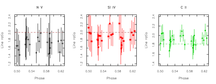
Figure 7: Ratio of lines of doublets of N V, Si IV and C II. The horizontal lines mark the expected values in optically thin plasma. Opacity effects are not detected.

The ratio of lines in doublets of Si IV, N V and C II are sensitive to opacity effects (Mathioudakis et al., 1999; Bloomfield et al., 2002). In optically thin plasma, the ratio of the pairs of lines is around 2 for the Si IV and N V, and $\sim 1.8$ for C II. Any departure from these values is suggesting that dense plasma is present. We have obtained the ratios for Si IV, N V and C II doublets for each exposure, and compared these with Chianti predictions (Fig. 7). We do not observe strong departures from the expected values (the scatter is within $1\sigma$ for most of the exposures). On average, N V ratios show systematic lower values and C II ratios show an excess with respect to the theoretical value, while Si IV ratios are in better agreement with the expected value of 2. No clear departure is found at the two brightenings. Overall, we conclude that the conditions for optically thin plasma are met during exposures, and the small systematic difference in N V and Si IV could be due to uncertainties in the atomic database.

3.2 Line variability

Two main episodes of flux variability are observed at phases $\phi\sim 0.525$ and $\phi\sim 0.59$, during exposures 5 and 14. We followed the evolution of the spectrum of HD 189733 during theses two exposures in more detail, accumulating three spectra from the photons recorded in three shorter time intervals of length $\sim 200$s, as described in Sect. 2. In Tables 3–5 we report the measurements obtained in these six time sub intervals of $\sim 200$s each (labelled with 5a, 5b, 5c, and 14a, 14b, 14c, respectively).

The line variability is significant at a level of $8-10\sigma$. The difference of variability at planetary transits and post eclipse phases is reminiscent of the different X-ray variability observed at transit and post eclipse phases Pillitteri et al. (2014a, 2011). This suggests the remarkable behavior of the transition region and the corona of HD 189733 after the planetary eclipse, and point to a major role of its hot Jupiter.

We discuss in more details each episode of variability in the next two sub-sections.

Figure 3: Fluxes of lines as a function of the planetary phases from spectra obtained during our program. The names and the wavelengths of the lines are indicated in each panel. The horizontal line represents the average stellar flux obtained from the first four spectra, i.e., when the planet is completely obscured by the star. Two main episodes of variability are observed at phases 0.525 and 0.588 with duration $t\leq 400$ s, for which we obtained sub-interval spectra (cross symbols).

Figure 4: As in Fig. 3, fluxes of lines as a function of the planetary phases from archival spectra obtained at the planetary transit. The names of lines are indicated on the top axis. The horizontal line represents the average stellar flux. Variability is observed at $\leq 3\sigma$ level only.

3.3 First flux increase

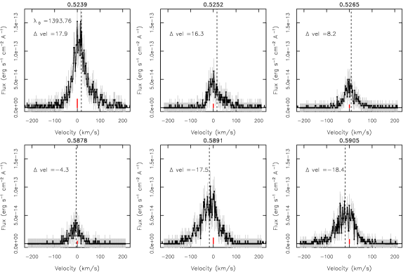
Figure 13: Line profiles of Si IV at 1393.7Å. We show here the spectra from the three sub-exposures of $\sim 200$ s 5a, 5b, 5c, 14a, 14b, 14c. The values of the planetary phases are indicated on the top axis of each panel. The vertical line marks the centroid of the line, the red segment is the rest line wavelength (value shown in the top left panel). The differences between centroid and rest wavelength in velocity space (km/s) are indicated in each panel (corrected for stellar radial velocity, RV = 2.6 km/s).

The line profiles of Si and C ions during time intervals 5a, 5b, 5c (top row), and 14a, 14b, 14c (bottom row) are plotted in Appendix (Figs. 13 through 19). We marked the centroid and the nominal positions of the lines. The figures shows in details the changes of flux, centroid and widths of these lines on a time scale of $\sim 200$ s.

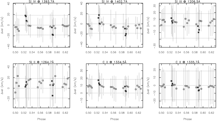
Figure 5: Centroids and FWHMs (vertical segments) of lines as a function of the planetary phases. The horizontal lines mark the values of $\pm 18.3$ km/s, i.e., the velocity of the sub-planetary point at the stellar surface co-moving with the planet. For Si ions the centroid shifts at phases 0.525 and 0.59 are quite close to these values. Filled symbols are the points from sub-interval spectra.

At the beginning of the exposure 5 (second orbit), the line fluxes are already elevated. The interval 5a is the first temporal segment in which we observed HD 189733 when the planet is appearing on view after its eclipse (see the schematic on Fig. 1, left panel, phase range = $0.523-0.527$). We were unable to observe the phases between 3rd and 4th contact, when the planet emerged after the eclipse, so the increase of the line fluxes could have started while the planet was emerging. The line fluxes decrease on a time scale of 400 s restoring to the basal level for the rest of the HST orbit and the subsequent one, until the second flux increase at phase $\sim 0.59$. Small variability is seen during the third HST orbit (Fig. 3), at a level of 2$\sigma$ variations, and of the same level of variability observed at the planetary transits.

Fig. 5 shows the line centroid shifts with respect to the line wavelength at rest (in km/s) and the FWHMs, as a function of the planetary phases. The uncertainties of centroids are estimated to be $\sim 4-5$ km/s. In the same plots, the horizontal lines correspond to the velocity of a point on the stellar surface co-moving with the planet orbital period. We also recall that the stellar period is comprised between 11.9d and 16d (Fares et al., 2010), corresponding to the velocities $2.5-3.4$ km/s and thus smaller than the speed of the point co-moving with the planet (18.3 km/s).

During the first increase of flux, the centroids of all ions but Si II at the peak of the brightening are shifted red-ward. For Si IV the pattern is the clearest, with velocity shifts consistent with the co-moving planetary speed. For C II line at 1334.5 Å the centroid of the line is systematically shifted toward $\sim+9$ km/s, and on top of this bias we observe the same pattern of shifts as in the case of Si IV lines. This systematic redshift is also seen in the archival spectra taken at the planetary transit. A more accurate de-blending analysis with IRAF shows that the lines of C II can be fitted with two Vogt profiles, one consistent with the RV shifted stellar wavelength, and the other profile red-shifted by $\sim 20-23$ km/s which is still consistent with the planetary co-moving speed (18.3 km/s), given the uncertainties of centroid estimates.

Similar results are obtained when using a cross-correlation technique with fxcor task in IRAF. First, we subtracted spectra of exposures 5a, 5b, 5c, and 14a, 14b, 14c from the average spectrum of the orbit I (after rebinning them a factor 4x of the original resolution). For each residual spectrum, a spectral portion around the C II and Si IV doublets was cross-correlated with the average spectrum of orbit I. We find that in exposures 5a, 5b, 5c the residual spectrum is red-shifted by up to $20\pm 5$ km/s, while in exposures 14a, 14b, 14c the residual spectra are blue-shifted of $-20\pm 5$ km/s with respect to the average, basal spectrum of orbit I.

3.4 Second flux increase

The second event of variability started at phase $\sim 0.588$ and lasted for about 400 s. It is weaker than the first event. Remarkably, this event along with the X-ray flares observed in 2009, 2011 and 2012 (Pillitteri et al., 2010, 2011, 2014a) occurred in a very restricted range of phases ($\phi\sim 0.52-0.6$). Fig. 5 shows that the lines and in particular Si IV and Si III during this brightening exhibit a remarkable blue-shift, with Si IV values similar to the planetary co-moving speed ($\sim-18$ km/s). The interpretation of this blue-shift is that hot material on the surface of the star, perhaps a hot spot at temperatures of $\sim 10^{5}K$, is co-moving with the planetary motion and emerging at the stellar limb.

In Fig. 8 we plot the empirical cumulative distribution functions (ECDFs) of the time-tagged events that compose three lines of different temperatures of formation, namely C II at 1334.5Å, Si IV at 1393.7Å, and N V at 1238.8Å. Fully exploiting the time tagging feature of COS, these curves allow us to evidence the timing of the line increases. The two sets of distributions are created for events accumulated within 0.5Å from the nominal line center, during exposures 5 and 14 (HST orbits II and IV) that host the two brightenings. During orbit II, the spectral lines start to brighten simultaneously, as demonstrated by the deviation from the purely constant rate (the linear ramp in dotted line). However, Si IV increases its flux faster than N V and C II lines during the first brightening. The second brightening shows different ECDF shapes: there is a delay between the onset of brightening in N V, Si IV and C II, with a peak of N V growth is at phase 0.588. N V line brightening starts earlier and at a faster rate than Si IV line. Here C II line starts last and it is the slowest, nearly exactly the opposite behavior than in the first brightening.

The nature of the two brightenings appears different: the first is a gradual event, almost simultaneous in the three lines, and less impulsive than the second one. The bulk of plasma temperature in this event is near the peak temperature of Si IV line, while relatively less plasma is present in the temperature range of the other two lines. The second event is an impulse, with hotter plasma appearing first (T$\geq$100,000 K), then in a sequence intermediate temperature plasma appears (60,000 K) and, eventually, plasma as cool as 30,000 K. The nature of this second event is plausible with a flaring episode due to an accreting event with a subsequent cooling of the plasma to return to the pre-flare thermal conditions. The analysis of the differential emission measure in the next sub-section helps to better understand the thermal structure of the plasma during quiescence and the two brightenings.

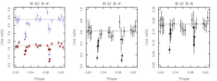
Figure 6: Top row: ratio of Si lines as a function of the planetary orbital phase. Filled symbols are the points from sub-interval spectra. Left panel: Si III / Si IV 1402.5Å(blue symbols), Si III / Si IV 1393.7Å(red symbols). Central panel: Si II / Si IV 1402.5Å. Right panel: Si II / Si III. Bottom row: temperature vs. planetary phase derived from line ratios. The comparison of the two peaks shows that the second brightening has been hotter in temperature than the first one.

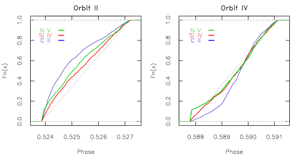
Figure 8: Empirical cumulative distribution functions of events of lines of C II 1334.5 Å (blue), Si IV 1393.7Å (red), and N V 1238.7Å (green). The curves refer to the orbits II (left panel) and IV (right panel) during the two line brightenings. A different rise of the lines is observed during the two brightenings, slowly rising the first one, hotter rapid and impulsive the second one.

3.5 Differential emission measure

The ion lines in the range of COS spectra have the peaks of formation temperatures typical of the transition region, in the range $T=10^{4}-8\times 10^{5}\mathrm{K}$ (Fig. 9). The emissivities are calculated by means of the CHIANTI database and a suite of Python routines ChiantiPy 0.5.2 (Dere et al., 1997; Landi et al., 2013). We investigated the thermal structure of the emitting plasma of HD 189733 by means of the differential emission measure (DEMs). DEMs give a measure of the volume and density of plasma emitting at a certain temperature, and they are calculated by estimating the lower envelope of the contribution of each line (dotted curves in Fig. 10). From the emissivity curves and line fluxes we obtained the DEMs for the quiescent part and the two impulsive events (solid thick lines in Fig. 10). The comparison of the values of the quiescent DEM and of the DEMs of the two brightenings, and the two slopes around the minimum (occurring at $\sim 8\times 10^{4}$ K) shows that during both events more plasma is contributing to the emitted spectrum in all the range of temperature. For the first event, the emitting plasma is denser and/or fills a bigger volume than in quiescent phase. During the second event the slope of the cool side of the DEM is flatter and steeper than in the quiescent DEM and the DEM of event 1. This means that relatively hotter plasma is present during event 2, and less hot plasma is visible during event 1, remarking again the different nature of the two brightenings as pointed out before by means of ECDFs. The slope of DEMs at high temperatures is poorly constrained, being only due to the contribution of N V doublet, and thus it is identical in all the three DEMs.

Figure 9: Emissivity of lines. in the spectral range $1150\AA-1450\AA$. Left: C II doublet. Center: Si II (dashed line), Si III (dot-dashed line) and Si IV doublet (solid line). Right: N V doublet. The curves are derived from CHIANTI database and ChiantiPy routines. The lines are formed in the range $2-50\times 10^{4}K$ and thus probe the temperatures typical of the transition region.

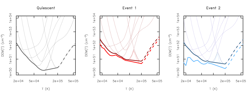
Figure 10: Differential emission measure (DEMs) of quiescent spectrum (left panel), first (central panel) and second brightening (right panel). The dotted curves are the contributions from each line. DEMs relative to event 1 and 2 are shown as total DEM (dark colored curve), and after subtraction of the quiescent DEM (light colored curve). For doublets of Si IV, N V and C II we used the sum of the line fluxes and emissivities. Above 2$\times 10^{5}$ K the curves are constrained only by N V.

3.6 Ly$\alpha$ and other lines

The main feature in the COS spectra is the H I Ly$\alpha$ line.  A detailed analysis of Ly$\alpha$ in spectra of solar type stars has been performed by Wood et al. (2005) and, for HD 189733, by Bourrier et al. (2013). Here we attempt to a qualitative description of the Ly$\alpha$ as observed with COS; however, a detailed quantitative analysis is beyond the scope of the paper.

The intrinsic Ly$\alpha$ emission of a star of spectral type of HD 189733 is difficult to assess because of the core absorption due to interstellar gas. Without the narrow geocoronal emission and the strong interstellar medium (ISM) absorption, the line would appear as a double peaked profile. The ISM absorption almost fully depletes the central part of the profile, and, in addition, deuterium absorption is present at -80 km/s. The contamination from geocoronal emission has a wavelength width comparable with the COS slit aperture and it is difficult to subtract (Linsky et al., 2010). Furthermore, the line shows a periodic change in intensity and profile shape as a function of the satellite orbital phase.

We subtracted the airglow emission from Ly$\alpha$ by using a spectrum obtained during program # 11999, which has been performed with the same COS setup used in our program. The airglow spectrum of Ly$\alpha$ has been smoothed with a spline function, corrected for the reflex satellite movement, and resampled on a grid of 0.04Å centered on the nominal line central wavelength (1215.67Å) in a range of $\pm 1.6\AA$ (394.5709 km/s). The profiles of our spectra were smoothed and resampled in the same way, the airglow spectrum was scaled to the median of the five bins around the central wavelength and subtracted to our spectra. The results offer a way to qualitative discuss the “decontaminated” Ly$\alpha$ of HD 189733 and compare the profile at the planetary transit and planetary eclipse.

We plot in Fig. 11 the profiles of Ly$\alpha$ of HD 189733 corrected for airglow emission, at three epochs, taken after a planetary eclipse and before a transit. We chose these phases as representative of the behavior of the line as a function of the airglow contamination. When the airglow emission is at its maximum (left panels in top and bottom rows), the correction suffers more of uncertainties, likely due to the saturation of the line peak in the detector. In the other cases, the correction seems more effective and the double peaked profile is recovered.  In almost all cases, the red peak is higher than the blue peak, as observed sometimes in other stars (see Fig. 6 of Wood et al., 2005) the reason is likely due to the shape of the interstellar absorption being more effective in the blue wing of the line while the extra deuterium absorption has a narrow effect in the blue portion at around -80 km/s (Bourrier et al., 2013; Lecavelier Des Etangs et al., 2010).

The average COS spectrum of HD 189733 (with an exposure of 12.106 ks) shows other small lines beside the Si, C, and N ion lines we have analyzed in details. Lines of Fe XII (1241.8Å and 1349.4Å) and Fe XIX (1328.8Å) are visible in the spectrum of the total exposure. These lines are from hot material composing the corona of HD 189733. A few very faint unidentified lines are present at 1274.95Å, 1289.9Å, 1359.2Å, and 1360.2Å.

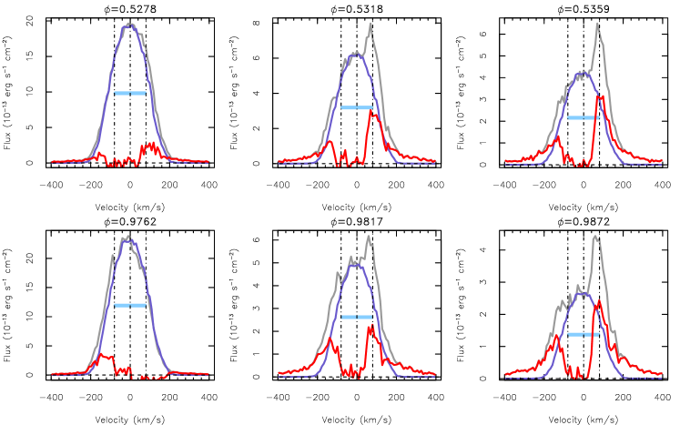
Figure 11: Examples of Ly$\alpha$ profiles corrected for the airglow emission in doppler shift velocities space. Orbital planetary phase is indicated on the top of each panel. Gray line is the raw profile, blue is the airglow contamination, red line is the corrected profile. Vertical lines mark the rest position, and $\pm 80$ km/s. The expected width of the uncontaminate and unabsorbed Ly$\alpha$ (150 km/s) is shown with  the light blue horizontal bar.

4 Discussion

We have observed HD 189733 for five consecutive orbits of HST during which the planet orbited through the phases $\phi\sim 0.5-0.63$. We obtained time resolved spectroscopy with COS around Ly$\alpha$ and we observed two intense line brightenings. A similar strong variability has been observed previously in the same phase range in X-rays (Pillitteri et al., 2010, 2011, 2014a). At these planetary phases the star systematically manifests an extraordinary rapid variability in the form of FUV brightenings and X-ray flares. While these events seem typical for an active star, the restricted phase range in which they manifest is anomalous and strongly points to an activity phased with the motion of the hot Jupiter around its host star. HD 189733 behaves markedly active when the planet is emerging from its eclipse. Of support to this phenomenon is the fact that multiple observations of HD 189733 obtained at the planetary transits both in FUV and X-rays (Poppenhaeger et al., 2013; Lecavelier Des Etangs et al., 2010) did not show similar levels of variability (being this of order of $\sim 2-3$ sigma level), and raising the question of why the star is more active when the planet is emerging from its eclipse.

In the following, we propose a scenario where the planet is inducing a relatively compact hot spot on the stellar surface, which benefits from limb brightening at specific post-eclipse phases. In particular,  we argue that such phased FUV brightenings and X-ray flares  could be likely the signature of star-planet interaction in the form of material evaporating from the planet, and accreting onto the star,  as suggested by recent 3D magneto-hydrodynamic (MHD) simulations by Matsakos et al. (2015), ( see also Cohen et al., 2011).  The numerical model is setup in PLUTO (Mignone et al., 2007, 2012), and includes a magnetized stellar wind, as well as a planetary outflow, with the stellar and planetary magnetic fields assumed to be $\sim$$2$ G and $\sim$$0.1$ G, respectively. The left panel of Fig. 12 shows a snapshot of such a simulation (polar view) in order to highlight the flow structure. In  this class of systems (Matsakos et al., 2015), submitted, for a classification of star–planet interactions), photo-evaporation drives a strong outflow from the surface of the Hot Jupiter, which becomes supersonic and collides with the stellar wind. The shocked material is slowed down by the surrounding stellar plasma, and is dragged inwards by gravity forming a spiral-shaped trajectory. As a result, the accreting flow impacts onto the stellar surface at a location that precedes the sub-planetary point.

The right panel of Fig. 12 shows a close-up of the accretion region. The effects of the stellar wind and gravity funnel the ionized stream through an almost radial trajectory towards the star (point A, right panel of Fig. 12). The motion of the infalling material is obstructed by the pressure (thermal plus magnetic) of the stellar corona at a finite height above the stellar surface (point B).  At that location, the flow forms a hot and dense structure (the “knee”), with number densities up to $10^{8}\,$cm^-3.  Recent planetary outflow models from Koskinen et al. (2013) suggest $6-10$ times higher mass loss rates than Murray-Clay et al. (2009), which would increase the knee density value found in our simulation. In addition, cooling mechanisms could also contribute to condense the gas. Note that the whole spiral-shaped stream corotates with the hot Jupiter, and hence, both points A and B rotate around the star with an angular velocity similar to that of the planetary orbit ($P_{\rm pl}\sim 2.2\,{\rm d}$). However, the material that accumulates in point B experiences the drag of the slower rotating star ($P_{*}=11.9\,{\rm d}$), and as a result, it loses its angular momentum and lags behind. In addition, the local pressure distribution pushes the gas to the right, leading to the formation of the “knee” structure highlighted in the right panel of Fig. 12. The material then accretes onto the star, impacting the chromosphere at point C.  A visual inspection suggests that point C precedes the location of the planet by about $70-90\deg$. As the planet orbits around the star, point C is continuously relocated, effectively corotating with the planet (but the accreted material should acquire the rotation of the star after the impact on the surface). Due to the weaker magnetic fields of Main Sequence stars, the accreting plasma is not expected to impact at high latitudes as in protostars.

For the discussion that follows, consider the observer (Earth) to be on the left side of Fig. 12 (the line of sight is depicted with an arrow in the left panel), thus observing the planet after its eclipse. At phase $\sim 0.52$, the elongated structure of hot material in point B is approximately aligned with the line of sight. Since the plasma motion is receding with respect to the observer with a velocity of $10$–$50\,\rm{km\,s}^{-1}$, its emission will appear redshifted. Shortly after, the impact region (point C) appears at the stellar limb along the line of sight. The hot spot moves towards the observer with the angular velocity of the planet, corresponding to a local speed of $15$–$20\,\rm{km\,s}^{-1}$ that will blueshift the emitted radiation.

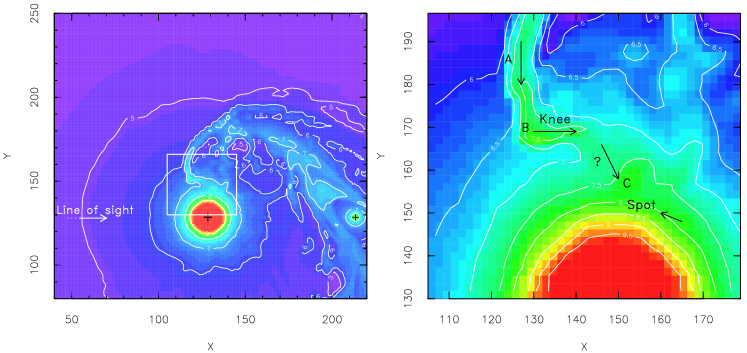
Figure 12: Particle density contours  (units cm^-3) of an MHD simulation that models star–planet interactions between a hot Jupiter and its host (polar view). The flow morphology provides a strong candidate scenario to address the FUV line variability of HD 189733 (the observer is viewing the system from the left side).  The star rotates counterclockwise, and the planet orbits the star along the same direction. The two “+” symbols shown on the left panel indicate the location of the star (red disk) and the planet (gr een disk). A close up of the impact region is depicted in the right panel, where the motion of the accreting plasma is marked with arrows. Specifically, the shocked plasma is funnelled by the magnetized stellar wind in an almost radial trajectory close to the star (A), it forms a “knee” structure that consists of hot and dense plasma (B), and then accretes in a spot ahead of the orbital phase (C). The precise details of accretion are not investigated by the simulation (zone marked with ?). The knee (B) of the stream and the active spot upon impact on the surface (C) are the main sites of production of the enhanced flux observed in FUV and X-rays that is phased with the orbital motion.

In this context, we find a plausible match between the accretion features in the MHD simulations and the FUV observations. The first brightening can be attributed to the knee coming into view approximately when the planet is emerging from the eclipse (point B). The observed redshift is in agreement with the simulation where the flow is receding along the line of sight. Because of the shock which is likely to form there, the gas in the knee is expected hotter than the average temperature of the transition region, but still cooler than the gas impacting on the surface of the star.

The second brightening can be attributed to the spot emerging later at the limb, which is due to the impact of the accreting gas onto the chromosphere. It is plausible to imagine that the accreting spot is forced to move with the co-moving speed of the planet at the stellar surface ($\sim 18.3$ km/s), since the stream inherits the angular speed of the orbit. As a result, a blueshift of the lines is observed because the spot is moving toward the observer, and at a rate that is faster than the rotational velocity of the stellar surface (3.4 km/s).

Note that secondary flows may detach from the main body of the stream and fall onto the surface with minor impacts. Nevertheless, the spot of the bulk accretion remains confined in a restricted range of planetary orbital phases, and remains within the range of phases in which we observed variability in XMM-Newton and in the present HST observations.

The accreting stream is moving in an elongated magnetized region (marked by points A and B of Fig. 12) that can host magnetic reconnection (and thus flaring activity). The relevant size is markedly different from the typical sizes of coronal loops of Main Sequence stars like the Sun. An estimate of the size of such long structures has been inferred from the analysis of the decay light curve of a flare observed in X-rays (Pillitteri et al., 2014a), and it is of a few stellar radii. From the simulations, we estimate that the stream forms an arc before the knee of the size of the $1.5-2$ stellar radii, and the knee is about $1.5$ stellar radii above the stellar surface. The mass flux through the knee is estimated of order of a few units of  $10^{-8}$ gr s^-1 cm^-2. From this mass flux, assuming an accreting tube with section of $0.1\times R_{*}$, we estimate a mass accretion from the planet of  $\sim 5\times 10^{18}$ gr yr^-1, or up to about  1% of a Jupiter mass in $\sim 4$ Gyr, if the accretion were steady during this period of time.

We warn that the numerical model does not have adequate resolution to model in detail the path of the plasma flowing from point B to C (limited by the demanding nature of 3D MHD simulations). The precise location of the spot (point C) may vary slightly due to the time-dependence of the plasma dynamics. It is plausible that the accretion is not happening in form of a continuous flow, but instead, the plasma accumulates until the density of the gas excedes the confining pressure of the magnetic field, and mimicks the fall of dense fragments observed just after the solar eruption of June 7 2011 (Reale et al., 2013, 2014). The limitations of the numerical simulation prevented us also from following in detail the impact onto the stellar surface. The surface is treated as a boundary which does not physically describe the chromosphere, but rather the base of the stellar wind.

Such MHD simulations of systems harboring hot Jupiters differ from previous simulations (e.g., Cohen et al., 2011) in the treatment of the stellar and planetary winds. They also differ from analytical models of purely magnetic star-planet interaction (Lanza, 2009; Lanza et al., 2010, 2011). However, all these modeling attempts concur to qualitatively describe a preferred planetary phase range in which stellar activity is enhanced by magnetic reconnection, or, by accreting material, as in the model presented above from Matsakos et al. (2015).

Stars accrete material from their circumstellar disks during the pre- Main Sequence phase, and, depending on the rate of accretion, they are identified as Classical T-Tauri ( CTTSs, strong accretors) and Weak-line T-Tauri (WTTSs, weak accretors). Given that we make the hypothesis that HD 189733 is accreting material from its hot Jupiter, a comparison between the spectrum of HD 189733 and CTTSs/WTTSs stars is in order. Ardila et al. (2013) present an extended and thorough analysis of FUV spectra of a sample of CTTSs and WTTSs. They recognize a broad and a narrow components in the C IV, Si IV and N V lines, with the relative weight of the narrow to broad component varying between 20% and 80% as a function of the accretion rate. The lines of WTTSs are shaped mainly by a low redshifted, narrow component. C IV lines are redshifted in both CTTSs and WTTSs, with the redshift being of order of 10 km/s in WTTSs. FUV lines of HD 189733 differ from those of CTTSs and WTTSs. In HD 189733 we observe narrow lines like in WTTSs and a systematic redshift of C II lines that is usually associated with emission from the gas flowing down in the coronal loops.

We find similarities between the spectral features of HD 189733 and the FUV spectrum of the solar eruption of June 7 2011. The solar event has been analyzed in detail by Reale et al. (2014). This unusual eruption showed the break of a dense filament that ejected dense fragments eventually falling down on the solar surface. The dynamics of this eruption is the best template for accreting events in pre Main Sequence stars (Reale et al., 2013) and, in our case, for HD 189733. The brightenings of C IV doublet at 1550Å were modeled by (Reale et al., 2014) by means of a cloud of fragments hitting the top of the chromosphere. Among the results, Reale et al. (2014) explain the broad component of FUV lines in accreting stars as due to the accretion taking place simultaneously at different locations on the stellar surface. They also do not find a continuum increase in the reconstructed spectra of the impacting fragments. In solar flares due to magnetic reconnection, a rise of the continuum flux is observed as due to the heating process and the rise of the free-bound and free-free contributions (Brekke et al., 1996).  The lack of continuum flux increase in the brightenings we observed in HD 189733 is analog to the solar behavior during the impacts of the dense fragments after their eruption. By means of ECDFs we have established in Sect. 3.4 that the second event has an impulsive nature. The lack of continuum increase during this brightening is analog to the lack of continuum increase in the solar event described above. This allows us to consider the second brightening in HD 189733 as an accretion event of planetary material similar to the solar event rather than a flare due to magnetic interaction and/or reconnection. On the other hand, the first event is rather due to the emergence of a hotter, elongated region (knee) briefly seen through a favorable line of sight.

On the wider context of systems with hot Jupiters, the conditions for establishing a steady accreting stream strongly depend on  the stellar wind, the intensity  and geometry of the stellar magnetic field, the stellar activity (related to the magnetic activity), and the separation of star and planet (which controls also the rate of evaporation of the planetary atmosphere). In this respect, HD 189733 demonstrates to be one of the most favorable systems where this phenomenon can be detected. The presence of a multi-year activity cycle  (see, e.g., Fares et al., 2013), associated with a variability of reconnection events (e.g. Llama et al., 2013), implies alternating periods of active accretion and periods of weak or absent accretion. As a consequence, an activity cycle would explain lack of systematic phased variability when observing stars after a few years, and the on/off behavior observed in the case of HD 179949 (Shkolnik et al., 2008).

We find unlikely that the two events are related to hot material emitting close to the planet. Such material should be ejected from the planet and inherit a velocity of at least 150 km/s which is the orbital velocity of the planet. Similar velocity should be involved in magnetic reconnection events close to the planet. At phases 0.52 and 0.59 the components of such velocity along the line of sight are $\geq-18$ km/s and $\geq-80$ km/s, respectively. In both cases we should see a blue shift when observing after the planetary eclipse. At phase 0.52 we observe a redshift of about +20 km/s, thus a difference of $\geq 40$ km/s with respect to the expected Doppler shift of emission from gas close to the planet. For the second event at phase 0.59, the expected blue shift of -80 km/s from material close to the planet. Such blue shift is not detected in any of the lines.

SPI events should be synced with the synodic period of the star+planet system which is about 2.7 days. This value is quite close to the orbital period of the planet, thus disentangling this effect from other effects purely related to the planetary motion is difficult. In addition it would require a continuous monitoring of the star for at least 3 synodic periods, which is a demanding observational effort not realized to date.

5 Conclusions

In this paper we have presented a time resolved spectroscopic analysis of the FUV spectrum of HD 189733 acquired with COS on board HST, around the Ly$\alpha$ line in the range 1150-1450Å. We have observed the phases after the planetary eclipse, for a duration of five HST orbits. The spectral range comprises several lines of ionized Si, C, N and O, which form in the range of temperature of $20,000-200,000$ K, typical of the transition region.

Two rapid line flux brightenings have been observed in Si, C, and N lines with a duration of $200-400$ s. No similar brightenings have been observed in archival observations of HD 189733 taken with the same instrument at a planetary transit. The first event happens when the planet is emerging after the eclipse (phase $\sim 0.52$), the second event later at phase $\sim 0.59$. From the line ratios of Si ions, and with a reconstruction of the differential emission measure, we followed the evolution of the plasma temperature and the rise of temperature during both events. The time evolution of the line fluxes is different and hint to a different nature of the two events: the evolution of the first event has been gradual within 400 s. The second event has been a rapid impulse observed first in the hot lines of N V, and then in the cooler lines of Si IV and C II. The second event has been also hotter than the first one. For the second event, we find a strong similarity with the impacts of dense fragments during the solar eruption of June 7 2011. In particular, both events are impulsive and lack of continuum increase, at odds with solar and stellar flares due to magnetic reconnection.

With the help of MHD simulations,  we argue that the spectroscopic sequence is the signature of gas that evaporates from the planet and accretes onto the star. In particular, the MHD simulations show that material  can effectively escape the planetary surface, becomes supersonic, and collides with the stellar wind. The interaction leads to the formation of an elongated spiral-shaped stream that precedes the planetary motion, and a cometary-type tail that trails the orbit. Near the star, the stream is funneled by the surrounding magnetized plasma, and infalls almost radially. The flow is then obstructed by the coronal pressure at a finite height above the stellar surface, possibly forming a shock. The dynamical evolution then leads to the formation of a “knee” structure of dense and hot plasma, that is subsequently channeled inwards and impacts onto the stellar surface. As a consequence, the knee region and the surface accretion spot are hotter and denser than the average transition region of the star. Since the entire accreting stream is co-rotating with the planet, the phased variability occurs when – under favorable alignment with the line of sight – the knee and the accretion spot emerge at the stellar limb. The phase angle between the accretion spot and the sub-planetary point matches quite well the observed phase lag in X-ray and FUV activity.

This scenario is appealing because it can explain both X-ray and FUV observation after the planetary eclipse. These observations provide the spectroscopic signatures of the accreting planetary gas. However, further monitoring at the post planetary eclipse phases  and on longer time baseline are needed to confirm the systematic occurrence of such spectroscopic signatures and the enhanced activity of HD 189733 at these particular phases.

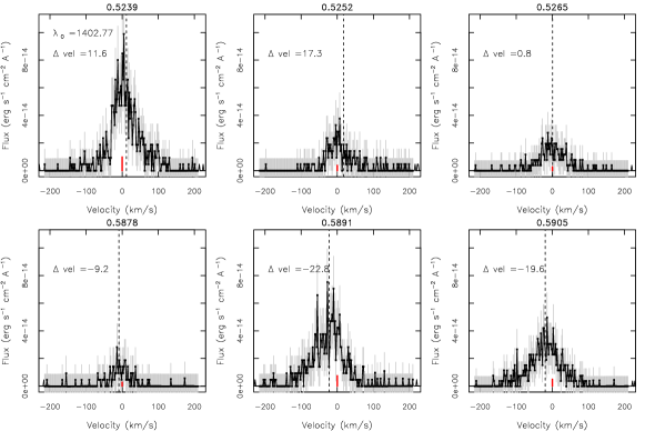
Figure 14: Same as in Fig. 13 for the Si IV line at 1402.8 Å.

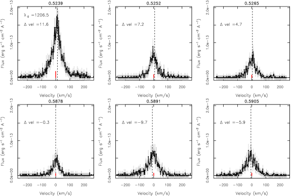
Figure 15: Same as in Fig. 13 for the Si III line at 1206.5Å.

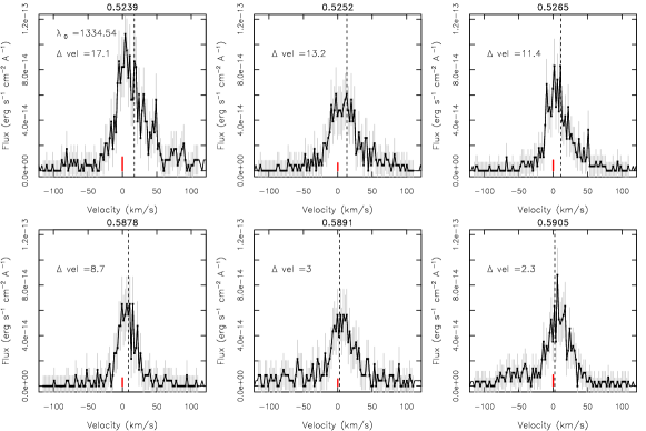
Figure 16: Same as in Fig. 13 for the C II line at 1334.5Å.

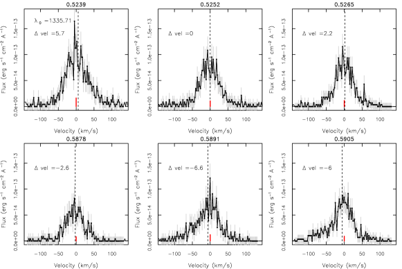
Figure 17: Same as in Fig. 13 for the C II line at 1335.7Å.

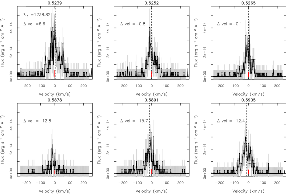
Figure 18: Same as in Fig. 13 for the N V line at 1238.8Å.

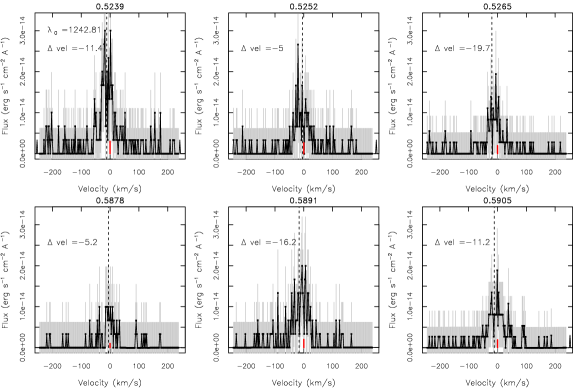
Figure 19: Same as in Fig. 13 for the N V line at 1242.8Å.

Table 3: Centroids, FWHMs and fluxes of Si IV and N V lines for each exposure.

Exposure	Wavelength	FWHM	Flux	Error	Wavelength	FWHM	Flux	Error	Wavelength	FWHM	Flux	Error
	Å	Å	$10^{-15}$ erg cm-2 s-1		Å	Å	$10^{-15}$ erg cm-2 s-1		Å	Å	$10^{-15}$ erg cm-2 s-1
	Si IV 1393.7 Å				Si IV 1402.7 Å				Si II 1264.7 Å
1	1393.74	0.10	7.13	0.76	1402.77	0.19	3.36	0.68	1264.70	0.18	2.10	0.46
2	1393.74	0.25	6.78	0.74	1402.75	0.19	3.41	0.67	1264.78	0.25	2.33	0.46
3	1393.72	0.19	6.42	0.73	1402.73	0.18	3.26	0.66	1264.84	0.40	1.89	0.44
4	1393.71	0.21	6.43	0.73	1402.72	0.13	3.63	0.67	1264.76	0.35	2.18	0.45
5	1393.83	0.23	23.16	0.78	1402.82	0.29	13.05	0.66	1264.77	0.33	3.01	0.35
5a	1393.84	0.26	45.62	2.14	1402.83	0.25	25.11	1.84	1264.75	0.17	3.69	0.97
5b	1393.83	0.17	14.62	1.61	1402.85	0.19	8.10	1.48	1264.76	0.44	2.84	0.94
5c	1393.80	0.21	11.56	1.33	1402.78	0.32	7.13	1.25	1264.79	0.52	2.59	0.79
6	1393.79	0.17	9.16	0.58	1402.77	0.29	4.79	0.51	1264.77	0.42	2.14	0.32
7	1393.75	0.16	7.21	0.55	1402.78	0.08	3.78	0.48	1264.80	0.32	2.10	0.32
8	1393.75	0.20	6.85	0.54	1402.77	0.14	3.83	0.49	1264.81	0.42	2.20	0.32
9	1393.73	0.17	6.40	0.54	1402.76	0.28	3.37	0.48	1264.75	0.39	2.02	0.32
10	1393.73	0.16	6.82	0.54	1402.74	0.06	3.07	0.48	1264.79	0.39	1.84	0.32
11	1393.73	0.16	7.86	0.56	1402.75	0.15	4.06	0.50	1264.78	0.10	2.10	0.32
12	1393.72	0.23	7.10	0.55	1402.74	0.30	3.63	0.49	1264.80	0.20	1.93	0.32
13	1393.74	0.22	6.36	0.53	1402.74	0.24	2.86	0.47	1264.76	0.37	2.23	0.33
14	1393.68	0.31	22.26	0.77	1402.68	0.30	13.45	0.66	1264.75	0.29	2.37	0.33
14a	1393.74	0.26	8.16	1.46	1402.73	0.11	4.36	1.39	1264.79	0.30	2.06	0.91
14b	1393.68	0.26	33.02	1.95	1402.67	0.29	20.76	1.76	1264.68	0.50	2.17	0.92
14c	1393.67	0.43	24.96	1.55	1402.68	0.59	14.91	1.40	1264.76	0.13	2.78	0.78
15	1393.75	0.14	8.13	0.57	1402.73	0.18	4.39	0.50	1264.77	0.35	2.04	0.32
16	1393.73	0.17	6.63	0.54	1402.75	0.16	3.73	0.49	1264.83	0.43	2.26	0.33
17	1393.76	0.12	6.58	0.54	1402.76	0.16	3.63	0.49	1264.75	0.45	2.33	0.33
18	1393.75	0.20	7.43	0.56	1402.73	0.20	3.73	0.49	1264.77	0.12	2.25	0.33
19	1393.75	0.15	6.18	0.53	1402.76	0.05	3.21	0.48	1264.77	0.09	2.00	0.32
20	1393.75	0.19	6.53	0.54	1402.73	0.25	3.21	0.48	1264.81	0.11	2.25	0.33

Table 4: Line measurements as in Table 3 for lines of Si III and C II doublet.

Exposure	Wavelength	FWHM	Flux	Error	Wavelength	FWHM	Flux	Error	Wavelength	FWHM	Flux	Error
	Å	Å	$10^{-15}$ erg cm-2 s-1		Å	Å	$10^{-15}$ erg cm-2 s-1		Å	Å	$10^{-15}$ erg cm-2 s-1
	Si III 1206.5 Å				C II 1334.6 Å				C II 1335.7 Å
1	1206.51	0.18	11.76	0.73	1334.57	0.10	9.45	0.65	1335.70	0.17	17.30	0.81
2	1206.54	0.13	11.31	0.71	1334.58	0.13	8.83	0.63	1335.71	0.21	18.00	0.81
3	1206.54	0.14	10.63	0.70	1334.57	0.09	8.59	0.64	1335.72	0.17	17.64	0.80
4	1206.53	0.19	12.35	0.73	1334.57	0.14	9.17	0.63	1335.70	0.17	17.52	0.80
5	1206.54	0.24	29.16	0.76	1334.60	0.15	15.87	0.60	1335.72	0.21	28.72	0.77
5a	1206.55	0.19	53.50	1.99	1334.61	0.25	21.74	1.44	1335.74	0.18	36.47	1.75
5b	1206.53	0.18	20.12	1.49	1334.59	0.16	13.61	1.26	1335.71	0.25	25.86	1.56
5c	1206.52	0.17	16.43	1.23	1334.59	0.14	12.86	1.08	1335.72	0.20	24.66	1.35
6	1206.54	0.25	14.97	0.59	1334.58	0.11	11.77	0.53	1335.71	0.19	21.99	0.68
7	1206.53	0.13	11.75	0.54	1334.58	0.15	10.39	0.52	1335.71	0.19	20.72	0.66
8	1206.52	0.25	11.74	0.55	1334.57	0.10	10.72	0.51	1335.69	0.20	20.50	0.66
9	1206.50	0.15	11.45	0.54	1334.57	0.10	8.98	0.48	1335.69	0.24	17.90	0.63
10	1206.54	0.14	11.14	0.54	1334.57	0.13	8.81	0.48	1335.71	0.23	18.42	0.64
11	1206.52	0.15	13.55	0.57	1334.56	0.15	9.81	0.52	1335.71	0.18	19.63	0.66
12	1206.54	0.16	12.31	0.55	1334.56	0.15	10.26	0.51	1335.70	0.20	18.54	0.64
13	1206.51	0.20	10.98	0.53	1334.56	0.09	9.19	0.49	1335.70	0.22	17.30	0.62
14	1206.48	0.25	19.60	0.65	1334.55	0.12	12.50	0.55	1335.69	0.22	22.31	0.69
14a	1206.50	0.17	12.22	1.34	1334.57	0.12	10.20	1.16	1335.70	0.23	17.75	1.40
14b	1206.46	0.34	24.29	1.57	1334.55	0.18	13.70	1.27	1335.68	0.13	24.51	1.54
14c	1206.48	0.33	21.79	1.31	1334.55	0.12	13.39	1.08	1335.68	0.21	24.22	1.33
15	1206.53	0.13	12.01	0.55	1334.58	0.11	9.29	0.51	1335.71	0.16	18.59	0.64
16	1206.53	0.12	12.22	0.55	1334.57	0.13	9.89	0.50	1335.69	0.21	17.83	0.63
17	1206.50	0.18	12.49	0.56	1334.56	0.12	9.37	0.49	1335.70	0.24	18.21	0.63
18	1206.52	0.16	12.47	0.56	1334.58	0.12	9.70	0.50	1335.71	0.21	18.44	0.64
19	1206.53	0.18	11.47	0.54	1334.57	0.17	8.83	0.50	1335.71	0.20	18.60	0.64
20	1206.54	0.17	10.56	0.53	1334.56	0.12	9.07	0.49	1335.70	0.22	17.65	0.63

Table 5: Line measurements as in Table 3 for lines of C III multiplet and N V doublet.

Exposure	Wavelength	FWHM	Flux	Error	Wavelength	FWHM	Flux	Error	Wavelength	FWHM	Flux	Error
	Å	Å	$10^{-15}$ erg cm-2 s-1		Å	Å	$10^{-15}$ erg cm-2 s-1		Å	Å	$10^{-15}$ erg cm-2 s-1
	C III 1175 Å				N V 1238.8 Å				N V 1242.7 Å
1	1175.71	0.85	10.21	0.96	1238.81	0.19	3.40	0.51	1242.73	0.32	2.05	0.47
2	1175.72	0.74	9.67	0.94	1238.81	0.12	3.54	0.50	1242.75	0.08	2.14	0.46
3	1175.71	0.96	9.17	0.93	1238.81	0.14	3.53	0.50	1242.71	0.16	2.27	0.47
4	1175.72	0.21	10.95	0.96	1238.84	0.18	3.19	0.50	1242.72	0.11	2.24	0.47
5	1175.73	0.96	36.63	1.02	1238.83	0.16	8.03	0.45	1242.76	0.15	4.54	0.39
5a	1175.73	1.56	64.92	2.71	1238.85	0.36	11.20	1.18	1242.76	0.16	6.63	1.07
5b	1175.70	0.22	25.84	2.14	1238.82	0.09	7.21	1.09	1242.79	0.09	3.96	1.00
5c	1175.75	1.03	22.07	1.79	1238.82	0.12	6.06	0.91	1242.72	0.16	3.28	0.83
6	1175.73	0.46	14.92	0.76	1238.80	0.25	4.95	0.39	1242.78	0.18	2.63	0.34
7	1175.73	0.82	12.43	0.73	1238.80	0.24	4.10	0.37	1242.76	0.21	2.26	0.34
8	1175.73	0.18	10.86	0.71	1238.83	0.15	3.99	0.38	1242.73	0.22	2.35	0.34
9	1175.67	0.20	9.39	0.69	1238.82	0.22	3.44	0.36	1242.67	0.19	2.32	0.34
10	1175.74	1.41	10.54	0.71	1238.81	0.23	3.75	0.37	1242.72	0.13	2.00	0.33
11	1175.67	0.33	12.84	0.74	1238.78	0.24	4.27	0.38	1242.80	0.09	2.41	0.34
12	1175.70	1.48	10.33	0.70	1238.82	0.22	3.75	0.38	1242.69	0.98	1.90	0.33
13	1175.68	1.11	9.70	0.69	1238.81	0.19	3.16	0.36	1242.71	0.18	1.81	0.33
14	1175.60	1.39	29.34	0.95	1238.77	0.21	5.70	0.41	1242.76	0.20	3.42	0.36
14a	1175.68	1.45	11.74	1.89	1238.77	0.09	3.09	0.98	1242.78	0.67	2.13	0.95
14b	1175.59	1.27	43.86	2.45	1238.76	0.17	6.59	1.08	1242.74	0.44	4.50	1.01
14c	1175.58	0.27	31.85	1.92	1238.77	0.33	7.09	0.91	1242.76	0.25	3.60	0.82
15	1175.72	0.08	13.33	0.75	1238.80	0.21	3.99	0.38	1242.75	0.28	2.49	0.34
16	1175.69	0.22	10.81	0.71	1238.83	0.14	3.91	0.38	1242.75	0.23	2.25	0.34
17	1175.70	0.12	10.90	0.71	1238.79	0.15	3.99	0.37	1242.76	0.16	2.24	0.34
18	1175.73	0.13	11.03	0.72	1238.80	0.08	3.85	0.37	1242.74	0.12	2.57	0.34
19	1175.70	1.37	10.05	0.70	1238.80	0.19	3.74	0.37	1242.75	0.18	2.09	0.33
20	1175.69	0.11	9.53	0.69	1238.81	0.16	3.48	0.37	1242.75	0.14	2.02	0.33

Facilities: HST (COS).

References

- Agol et al. (2010) Agol, E., Cowan, N. B., Knutson, H. A., et al. 2010, ApJ, 721, 1861
- Ardila et al. (2013) Ardila, D. R., Herczeg, G. J., Gregory, S. G., et al. 2013, ApJS, 207, 1
- Ben-Jaffel & Ballester (2013) Ben-Jaffel, L., & Ballester, G. E. 2013, A&A, 553, A52
- Bloomfield et al. (2002) Bloomfield, D. S., Mathioudakis, M., Christian, D. J., Keenan, F. P., & Linsky, J. L. 2002, A&A, 390, 219
- Bouchy et al. (2005) Bouchy, F., Udry, S., Mayor, M., et al. 2005, A&A, 444, L15
- Bourrier et al. (2013) Bourrier, V., Lecavelier des Etangs, A., Dupuy, H., et al. 2013, A&A, 551, A63
- Bouvier (2008) Bouvier, J. 2008, A&A, 489, L53
- Brekke et al. (1996) Brekke, P., Rottman, G. J., Fontenla, J., & Judge, P. G. 1996, ApJ, 468, 418
- Cohen et al. (2009) Cohen, O., Drake, J. J., Kashyap, V. L., et al. 2009, ApJ, 704, L85
- Cohen et al. (2010) Cohen, O., Drake, J. J., Kashyap, V. L., Sokolov, I. V., & Gombosi, T. I. 2010, ApJ, 723, L64
- Cohen et al. (2011) Cohen, O., Kashyap, V. L., Drake, J. J., et al. 2011, ApJ, 733, 67
- Cuntz et al. (2000) Cuntz, M., Saar, S. H., & Musielak, Z. E. 2000, ApJ, 533, L151
- Delgado Mena et al. (2014) Delgado Mena, E., Israelian, G., González Hernández, J. I., et al. 2014, A&A, 562, A92
- Dere et al. (1997) Dere, K. P., Landi, E., Mason, H. E., Monsignori Fossi, B. C., & Young, P. R. 1997, A&AS, 125, 149
- Fares et al. (2013) Fares, R., Moutou, C., Donati, J.-F., et al. 2013, MNRAS, 435, 1451
- Fares et al. (2010) Fares, R., Donati, J.-F., Moutou, C., et al. 2010, MNRAS, 406, 409
- Gonzalez (2008) Gonzalez, G. 2008, MNRAS, 386, 928
- Israelian et al. (2004) Israelian, G., Santos, N. C., Mayor, M., & Rebolo, R. 2004, A&A, 414, 601
- Kopp et al. (2011) Kopp, A., Schilp, S., & Preusse, S. 2011, ApJ, 729, 116
- Koskinen et al. (2013) Koskinen, T. T., Harris, M. J., Yelle, R. V., & Lavvas, P. 2013, Icarus, 226, 1678
- Kramida et al. (2014) Kramida, A., Yu. Ralchenko, Reader, J., & and NIST ASD Team. 2014, NIST Atomic Spectra Database (ver. 5.2), [Online]. Available: http://physics.nist.gov/asd [2014, November 13]. National Institute of Standards and Technology, Gaithersburg, MD.
- Landi et al. (2013) Landi, E., Young, P. R., Dere, K. P., Del Zanna, G., & Mason, H. E. 2013, ApJ, 763, 86
- Lanza (2009) Lanza, A. F. 2009, A&A, 505, 339
- Lanza (2012) —. 2012, A&A, 544, A23
- Lanza et al. (2010) Lanza, A. F., Bonomo, A. S., Moutou, C., et al. 2010, A&A, 520, A53
- Lanza et al. (2011) Lanza, A. F., Bonomo, A. S., Pagano, I., et al. 2011, A&A, 525, A14
- Lecavelier des Etangs et al. (2004) Lecavelier des Etangs, A., Vidal-Madjar, A., McConnell, J. C., & Hébrard, G. 2004, A&A, 418, L1
- Lecavelier Des Etangs et al. (2010) Lecavelier Des Etangs, A., Ehrenreich, D., Vidal-Madjar, A., et al. 2010, A&A, 514, A72
- Lecavelier des Etangs et al. (2012) Lecavelier des Etangs, A., Bourrier, V., Wheatley, P. J., et al. 2012, A&A, 543, L4
- Linsky et al. (2010) Linsky, J. L., Yang, H., France, K., et al. 2010, ApJ, 717, 1291
- Llama et al. (2013) Llama, J., Vidotto, A. A., Jardine, M., et al. 2013, MNRAS, 436, 2179
- Mathioudakis et al. (1999) Mathioudakis, M., McKenny, J., Keenan, F. P., Williams, D. R., & Phillips, K. J. H. 1999, A&A, 351, L23
- Matsakos et al. (2015) Matsakos, T., Uribe, A., & Königl, A. 2015, ArXiv e-prints, arXiv:1503.03551
- Mignone et al. (2007) Mignone, A., Bodo, G., Massaglia, S., et al. 2007, ApJS, 170, 228
- Mignone et al. (2012) Mignone, A., Zanni, C., Tzeferacos, P., et al. 2012, ApJS, 198, 7
- Murray-Clay et al. (2009) Murray-Clay, R. A., Chiang, E. I., & Murray, N. 2009, ApJ, 693, 23
- Pillitteri et al. (2011) Pillitteri, I., Günther, H. M., Wolk, S. J., Kashyap, V. L., & Cohen, O. 2011, ApJ, 741, L18
- Pillitteri et al. (2010) Pillitteri, I., Wolk, S. J., Cohen, O., et al. 2010, ApJ, 722, 1216
- Pillitteri et al. (2014a) Pillitteri, I., Wolk, S. J., Lopez-Santiago, J., et al. 2014a, ApJ, 785, 145
- Pillitteri et al. (2014b) Pillitteri, I., Wolk, S. J., Sciortino, S., & Antoci, V. 2014b, A&A, 567, A128
- Poppenhaeger et al. (2013) Poppenhaeger, K., Schmitt, J. H. M. M., & Wolk, S. J. 2013, ArXiv e-prints, arXiv:1306.2311
- Poppenhaeger & Wolk (2014) Poppenhaeger, K., & Wolk, S. J. 2014, A&A, 565, L1
- Preusse et al. (2006) Preusse, S., Kopp, A., Büchner, J., & Motschmann, U. 2006, A&A, 460, 317
- Reale et al. (2014) Reale, F., Orlando, S., Testa, P., Landi, E., & Schrijver, C. J. 2014, ApJ, 797, L5
- Reale et al. (2013) Reale, F., Orlando, S., Testa, P., et al. 2013, Science, 341, 251
- Saar et al. (2004) Saar, S. H., Cuntz, M., & Shkolnik, E. 2004, in IAU Symposium, Vol. 219, Stars as Suns : Activity, Evolution and Planets, ed. A. K. Dupree & A. O. Benz, 355–+
- Schröter et al. (2011) Schröter, S., Czesla, S., Wolter, U., et al. 2011, A&A, 532, A3+
- Shkolnik et al. (2008) Shkolnik, E., Bohlender, D. A., Walker, G. A. H., & Collier Cameron, A. 2008, ApJ, 676, 628
- Shkolnik et al. (2003) Shkolnik, E., Walker, G. A. H., & Bohlender, D. A. 2003, ApJ, 597, 1092
- Shkolnik et al. (2005) Shkolnik, E., Walker, G. A. H., Bohlender, D. A., Gu, P., & Kürster, M. 2005, ApJ, 622, 1075
- Triaud et al. (2009) Triaud, A. H. M. J., Queloz, D., Bouchy, F., et al. 2009, A&A, 506, 377
- Vidal-Madjar et al. (2003) Vidal-Madjar, A., Lecavelier des Etangs, A., Désert, J.-M., et al. 2003, Nature, 422, 143
- Walker et al. (2008) Walker, G. A. H., Croll, B., Matthews, J. M., et al. 2008, A&A, 482, 691
- Wood et al. (2005) Wood, B. E., Redfield, S., Linsky, J. L., Müller, H.-R., & Zank, G. P. 2005, ApJS, 159, 118