Immiscibile two-component Bose Einstein condensates beyond mean-field approximation: phase transitions and rotational response

Abstract

We consider a two-component immiscible Bose-Einstein condensate with dominating intra-species repulsive density-density interactions. In the ground-state phase of such a system only one condensates is present. This can be viewed as a spontaneous breakdown of $\mathbb{Z}_{2}$ symmetry. We study the phase diagram of the system at finite temperature beyond mean-field approximation. In the absence of rotation, we show that the system undergoes a first order phase transition from this ground state to a miscible two-component normal fluid as temperature is increased. In the presence of rotation, the system features a competition between vortex-vortex interaction and short range density-density interactions. This leads to a rotation-driven “mixing” phase transition in a spatially inhomogeneous state with additional broken $\mathrm{U}(1)$ symmetry. Thermal fluctuations in this state lead to nematic two-component sheets of vortex liquids. At sufficiently strong inter-component interaction, we find that the superfluid and $\mathbb{Z}_{2}$ phase transitions split. This results in the formation of an intermediate state which breaks only $\mathbb{Z}_{2}$ symmetry. It represents two phase separated normal fluids with density imbalance.

I Introduction

Bose Einstein condensates (BECs) serve as highly useful synthetic model systems for a wide variety of real condensed matter systems, due to their tunable interactions using magnetic and optical Feshbach-resonances. By creating mixtures of the same boson in different hyperfine states, one effectively creates multicomponent condensates Myatt et al. (1997); Modugno et al. (2002); Thalhammer et al. (2008); McCarron et al. (2011). Furthermore, by using crossed lasers, one may set up lattice model systems with a vast combinations of intersite hopping matrix elements, as well as intrasite interactions, both intra- and interspeciesRaithel et al. (1997); Müller-Seydlitz et al. (1997); Hamann et al. (1998); Friebel et al. (1998); Guidoni and Verkerk (1998); Catani et al. (2008). This means that these model systems, apart from being interesting in their own right, emulate various aspects of a plethora of condensed matter systems of great current interest, such as multicomponent superconductors, Mott-insulators, and even topologically nontrivial band insulators. The latter follows from the recent realization of synthetic spin-orbit couplings in such condensates Lin et al. (2009a, b); Galitski and Spielman (2013). Of particular interest is the physics of these systems in the strong coupling regime.

Spinor condensates with two components of the order parameter represent a first step away from ordinary single-component condensates. This extension opens up a whole vista of physics which has no counterpart compared to single-component condensates, due to the wide variety of interspecies couplings that may be generated. Thus, these synthetic systems display physics which is beyond what is ordinarily seen in condensed matter systems.

The parameter range where inter-component density-density interactions exceed intra-component density-density interactions signals the onset of immiscibility, or phase separation, of the two components. Numerical works solving the Gross-Pitaevskii ground-state equations have also found interesting vortex lattices in this regime Kasamatsu et al. (2003, 2013); Tojo et al. (2010); Cipriani and Nitta (2013); Catelani and Yuzbashyan (2010); Mueller and Ho (2002); Filatrella et al. (2014); Kuopanportti et al. (2012); Battye et al. (2002). The effect of the repulsive inter-component interactions overpowering the intra-component interactions causes the condensate to form intertwined sheets of vorticesKasamatsu and Tsubota (2009). The condition for immiscibility is readily realized experimentally, using magnetic and optical Feschbach resonancesPapp et al. (2008); Tojo et al. (2010).

In this paper, we present results of large-scale Monte-Carlo simulations of a two-component Bose Einstein condensate at finite temperature. In a previous work, we have considered in detail the effect of thermal fluctuations for the case where the inter-component density-density interaction is less than or equal to the intra-component interaction Galteland et al. (2015). In the present paper, we focus on the regime of density-density interactions where the inter-component interactions is larger than the intra-component interactions. This regime is qualitatively different from the case in which the intra-component interactions dominate.

Previous works have studied the effect of an inter-component density-density interaction on the rotation-induced non-homogeneous ground states. These works were mostly limited to two spatial dimensions solving the Gross-Pitaevskii ground-state equations Kasamatsu et al. (2003, 2013); Tojo et al. (2010); Cipriani and Nitta (2013); Catelani and Yuzbashyan (2010); Mueller and Ho (2002); Filatrella et al. (2014); Kuopanportti et al. (2012); Battye et al. (2002); Kasamatsu and Tsubota (2009). although certain aspects of the three-dimensional case were also studied at mean-field level Kasamatsu et al. (2013); Battye et al. (2002). Here, we extend previous works in the immiscible regime to the case of finite temperatures and higher dimensions, including the full spectrum of density and phase-fluctuation of the condensate ordering fields.

II Definitions

II.1 Model

We consider a general Ginzburg-Landau(GL) model of an $N$-component Bose-Einstein condensate, which in the thermodynamic limit is defined as

$$\mathcal{Z}=\int\prod_{i}^{N}\mathcal{D}\psi_{i}\text{e}^{-\beta H},$$ (1)

where

$$H=\int d^{3}r\Bigg{[} \sum_{i=1}^{N}\sum_{\mu=1}^{3}\frac{\hbar^{2}}{2m_{i}}\left|(\partial_{\mu}-\mathrm{i}\frac{2\pi}{\Phi_{0}}A_{\mu})\psi_{i}\right|^{2}$$

$$+\sum_{i}^{N}\alpha_{i}\left|\psi_{i}\right|^{2}+\sum_{i,j=1}^{N}g_{ij}\left|\psi_{i}\right|^{2}\left|\psi_{j}\right|^{2}\Bigg{]}$$ (2)

is the Hamiltonian. Here, the field $A_{\mu}$ formally appears as a non-fluctuating gauge-field and parametrizes the angular velocity of the system. The fields $\psi_{i}$ are dimensionfull complex fields, $i$ and $j$ are indices running from $1$ to $N$ denoting the component of the order parameter (a “color” index), $\alpha_{i}$ and $g_{ij}$ are Ginzburg-Landau parameters, $\Phi_{0}$ is the coupling constant to the rotation-induced vector potential, and $m_{i}$ is the particle mass of species $i$. For mixtures consisting of different atoms or different isotopes of one atom, the masses will depend on the index $i$, while for mixtures consisting of same atoms in different hyperfine states, the masses are equal among the components $i$. The inter- and intra-component coupling parameters $g_{ij}$ are related to real inter- and intra-component scattering lengths, $a_{ij}$, in the following way

$$g_{ii} =\frac{4\pi\hbar^{2}a_{ii}}{m_{i}},$$ (3)

$$g_{ij} =\frac{2\pi\hbar^{2}a_{ij}}{m_{ij}};(i\neq j).$$ (4)

Here, $m_{ij}=m_{i}~{}m_{j}/(m_{i}+m_{j})$ is the reduced mass. In this work, we focus on using BECs of homonuclear gases with several components in different hyperfine states, i.e. $m_{i}=m\,\forall\,i$. The system we primarily have in mind is a mixture of Rb⁸⁷ atoms in two different hyperfine states $F=0$ and $F=1$, such that $N=2$. Note that when $g_{12}=g_{21}\equiv\lambda g>g_{11}=g_{22}\equiv g$, i.e. $\lambda>1$, there is a strong tendency in the system to phase separate, leading to two immiscible quantum fluids. For a homonuclear binary mixture, such as the mixture of Rb⁸⁷ atoms mentioned above, we have $m_{ij}=m_{i}/2$. Then, it suffices that $a_{ij}>a_{ii}$ for the inter-component density-density interactions to dominate the intra-component density-density interactions.

In the following, we have introduced dimensionless coupling parameters and fields, following Appendix A of Ref. Galteland et al., 2015. It is convenient to rewrite the potential (repeated indices are summed over)

$$V\equiv\alpha_{i}~{}|\psi_{i}|^{2}+g_{ij}\left|\psi_{i}\right|^{2}\left|\psi_{j}\right|^{2},$$ (5)

by introducing interaction parameters $\eta,\omega$, such that $g=\eta+\omega$, and $\lambda g=\eta-\omega$, i.e. $\eta=g(1+\lambda)/2$, $\omega=g(1-\lambda)/2$. Here, $\lambda$ denotes the ratio between the inter- and intra-component interactions. Then, Eq. 5 takes the form (up to an additive constant)

$$V = (\alpha_{1}+2\eta)|\psi_{1}|^{2}+(\alpha_{2}+2\eta)|\psi_{2}|^{2}$$ (6)

$$+ \eta(|\psi_{1}|^{2}+|\psi_{2}|^{2}-1)^{2}+\omega(|\psi_{1}|^{2}-|\psi_{2}|^{2})^{2}.$$

For $\lambda>1$, $\omega<0$, with the proviso that $\eta+\omega=\eta-|\omega|>0$ for stability. Furthermore, we will assume that $\alpha_{1}=\alpha_{2}$, such that $\langle|\psi_{1}|^{2}\rangle=\langle|\psi_{2}|^{2}\rangle$ when $\omega\geq 0$. ($\alpha_{1}\neq\alpha_{2}$ would act as an external field conjugate to the pseudo-magnetization of the system, and would destroy the Ising-like phase transition we report on below).

Conversely, for a binary mixture of homonuclear cold atoms, one may express the ratios of intra- to inter-component scattering lengths in terms of $\omega$ and $\eta$, as follows

$$\frac{a_{12}}{a_{11}}=\frac{1-{\omega}/{\eta}}{1+{\omega}/{\eta}}.$$ (7)

Note that the ratio of the scattering lengths only depend on the ratio $\omega/\eta$.

We discretize the model on a cubic lattice with sides $L$ by defining the order parameter field on a discrete set of coordinates $\psi_{i}(\mathbf{r})\rightarrow\psi_{\mathbf{r},i}$, $\mathbf{r}\in(i\hat{\mathbf{x}}+j\hat{\mathbf{y}}+k\hat{\mathbf{z}}|\,i,j,k=1,\ldots,L)$. The covariant derivative is replaced by a forward difference,

$$D_{\mu}\psi_{i}(\mathbf{r})\rightarrow\frac{1}{a}\bigg{(}\psi_{\mathbf{r}+a\hat{\bm{\mu}},i}\text{e}^{-\mathrm{i}aA_{\mu,\mathbf{r}}}-\psi_{\mathbf{r},i}\bigg{)}.$$ (8)

Here, the lattice version of the non-fluctuating gauge field is parametrized in Landau gauge, $A_{\mu,\mathbf{r}}=(0,2\pi fx,0)$, where $f$ is the number of vortices per plaquette, or filling fraction. The lattice spacing, $a$, is fixed to be smaller than the characteristic length scale of the variations of the order parameter, and $\hat{\bm{\mu}}\in(\hat{\mathbf{x}},\hat{\mathbf{y}},\hat{\mathbf{z}})$ is a unit vector.

Thus, the lattice version of the Hamiltonian we consider is given by

$$H=- \sum_{\begin{subarray}{c}\mathbf{r},\hat{\bm{\mu}}\\ i\end{subarray}}\big{|}\psi_{\mathbf{r}+\hat{\bm{\mu}},i}\big{|}\big{|}\psi_{\mathbf{r},i}\big{|}\cos(\theta_{\mathbf{r}+\hat{\bm{\mu}},i}-\theta_{\mathbf{r},i}-A_{\mu,\mathbf{r}})$$

$$+ \sum_{\begin{subarray}{c}\mathbf{r},i\end{subarray}}(\alpha_{i}+2\eta)~{}\big{|}\psi_{\mathbf{r},i}\big{|}^{2}$$

$$+ \sum_{\mathbf{r}}\eta{(\left|\psi_{\mathbf{r},1}\right|^{2}+\left|\psi_{\mathbf{r},2}\right|^{2}-1)}^{2}$$

$$+ \sum_{\mathbf{r}}\omega{(\left|\psi_{\mathbf{r},1}\right|^{2}-\left|\psi_{\mathbf{r},2}\right|^{2})}^{2}.$$ (9)

Here, we have written the order parameter fields as real amplitudes and phases, $\psi_{\mathbf{r},i}=\left|\psi_{\mathbf{r},i}\right|\text{e}^{i\theta_{\mathbf{r},i}}$. In addition, we have defined an energy scale, $J_{0}=\alpha_{0}^{2}a^{3}/g_{0}^{3}$, where $\alpha_{0}$ and $g_{0}$ are the parameters of the Ginzburg-Landau theory at $T=0$. Throughout, we fix $\eta=5.0$ and $\alpha_{1}+2\eta=\alpha_{2}+2\eta=0$. This guarantees a non-zero ground state condensate density for all values of $\eta$.

II.2 Ground state symmetry

Eq. 9 defines two superfluids coupled by density-density interactions. When there is no phase separation, we have a $\mathrm{U}(1)\times\mathrm{U}(1)$ symmetry broken in the ground state. When the inter-component interaction is equal to the intra-component interaction the system breaks $SU(2)$ symmetry. Here, we are interested in the phase separated case. In this case, the system breaks an additional $\mathbb{Z}_{2}$ symmetry, corresponding to interchanging $\psi_{1}\leftrightarrow\psi_{2}$. That is, when $\omega>0$, $|\psi_{1}|^{2}=|\psi_{2}|^{2}$ is favored. This represents a $\mathbb{Z}_{2}$ -symmetric state. On the other hand, when $\omega<0$, $|\psi_{1}|^{2}\neq|\psi_{2}|^{2}$ is favored, such that $|\psi_{1}|^{2}-|\psi_{2}|^{2}$ may acquire a nonzero expectation value, with equal probabilities that the expectation value is either positive or negative. This corresponds to breaking an Ising-like $\mathbb{Z}_{2}$ symmetry. Thus, the ground state breaks a composite $U(1)\times Z_{2}$ symmetry.

II.3 Observables

The equilibrium phases the model are characterized by several order parameters. To identify the Ising-like, phase separated order of the system we define

$$\Delta=\left|\langle\left|\psi_{1}\right|^{2}\rangle-\langle\left|\psi_{2}\right|^{2}\rangle\right|,$$ (10)

where $\langle\left|\psi_{i}\right|^{2}\rangle$ is the thermal and spatial average of $\left|\psi_{i}(\mathbf{r})\right|^{2}$

$$\langle\left|\psi_{i}\right|^{2}\rangle=\langle\frac{1}{L^{3}}\sum_{\mathbf{r}}\left|\psi_{i,\mathbf{r}}\right|^{2}\rangle.$$ (11)

A finite value of $\Delta$ signals relative density depletion in either of the condensates. In addition to $\mathbb{Z}_{2}$ order, it is important to monitor the $\mathrm{U}(1)$ ordering of the system. The helicity modulus measures phase coherence along a given direction of the system. It is defined as

$$\Upsilon_{\mu,i}=\frac{1}{L^{3}}\frac{\partial^{2}F[\theta^{\prime}]}{\partial\delta^{2}_{\mu}}\Bigg{|}_{\delta_{\mu}=0}.$$ (12)

Here, $F[\theta^{\prime}]$ is the free energy with an infinitesimal phase twist, $\delta_{\mu}$, applied along the $\mu$-direction, i.e., we make the replacement

$$\theta_{\mathbf{r},i}\rightarrow\theta_{\mathbf{r},i}^{\prime}=\theta_{\mathbf{r},i}-\bm{\delta}\cdot{\bf r}$$ (13)

in $F$.

We also identify the nature of the phases by computing thermal averages of real-space configurations of densities $\langle\left|\psi_{i}(\mathbf{r}_{\perp})\right|^{2}\rangle$ and vortices $\langle\left|n_{i}(\mathbf{r}_{\perp})\right|^{2}\rangle$ in the system. These are computed by averaging the quantity along the $z$-direction of the system, with subsequent thermal averaging. That is,

$$\langle n_{i}(\mathbf{r}_{\perp})\rangle=\langle\frac{1}{L_{z}}\sum_{z}n_{i,\mathbf{r}}\rangle.$$ (14)

and

$$\langle\left|\psi_{i}(\mathbf{r}_{\perp})\right|^{2}\rangle=\langle\frac{1}{L_{z}}\sum_{z}\left|\psi_{i,\mathbf{r}}\right|^{2}\rangle.$$ (15)

The vorticity, $n_{i,\mathbf{r}}$ is calculated by traversing a plaquette with surface normal in the $z$-direction, adding the phase difference $\theta_{\mathbf{r}+\hat{\bm{\mu}},i}-\theta_{\mathbf{r},i}-A_{\mu,\mathbf{r}}$ on each link. If this plaquette sum turns out to have a value outside the primary interval, $(-\pi,\pi]$, $2n\pi(-2n\pi)$ is added to the sum, which inserts a vortex of charge $+n(-n)$ on the plaquette.

To further characterize vortex structures, we examine the structure factor of the vortices, defined as

$$S_{i}({\bf q}_{\perp})=\Bigg{\langle}\left|\frac{1}{L^{3}f}\sum_{\mathbf{r}_{\perp},z}n_{i,\mathbf{r}}e^{i{\bf q}_{\perp}\cdot\mathbf{r}_{\perp}}\right|^{2}\Bigg{\rangle}.$$ (16)

This is simply the Fourier-transform of the $z$-averaged vorticity. To improve the resolution of the interesting $q$-vectors, we remove the $\bf{q}_{\perp}=0$ point from the figures. We also compute the specific heat capacity

$$\frac{C_{V}L^{3}}{\beta^{2}}=\langle{(H-\langle H\rangle)}^{2}\rangle.$$ (17)

as a means of precisely locating the various transition points.

II.4 Details of the Monte-Carlo simulations

We consider the model on a lattice of size $L_{x}\times L_{y}\times L_{z}$, using the Monte-Carlo algorithm, with a simple restricted update scheme of each physical variable, and Metropolis-Hastings Metropolis et al. (1953); Hastings (1970) tests for acceptance. Here, $L_{i}$ is the linear extent of the system in the Cartesian direction $i\in(x,y,z)$. In all our simulation, we have used cubic systems $L_{x}=L_{y}=L_{z}=L$, with $L\in\{24,32,40,48,56,64,96,128\}$. At each inverse temperature, $10^{6}$ Monte-Carlo steps are typically used, while $10^{5}$ additional sweeps are used for equilibration. Each Monte-Carlo step consists of an attempt to update each amplitude and phase separately in succession, at each lattice site. To improve acceptance rates, we only allow each update to change a variable within a limited interval around the previous value, the size of which is chosen by approximately maximizing acceptance rates and minimizing autocorrelations. The Mersenne-Twister algorithm is used to generate the pseudo-random numbers neededMatsumoto and Nishimura (1998). To ensure that the state is properly equilibrated, time series of the internal energy measured during equilibration are examined for convergence. To avoid metastable states, we make sure that several simulations with identical parameters and different initial seeds of the random number generator anneals to the same state. Measurements are post-processed with multiple histogram reweightingFerrenberg and Swendsen (1989). Error estimates are determined by the jackknife methodBerg (1992).

III Phase diagram in the absence of rotation

The model has a $\mathrm{U}(1)\times\mathrm{U}(1)\times\mathbb{Z}_{2}$ symmetry and hence the possibility for several phase transitions. However, for the parameter set which was simulated a single first-order phase transition is found, as we illustrate below for $\omega=-2$. For $f=0$, we have considered $L\in\{24,32,40,48,56,64\}$, and we present the results for $L=64$.

Fig. 1 shows the specific heat, Ising order parameter $\Delta$, and helicity moduli (phase-stiffness or equivalently superfluid density) of both components for $L=64$ and $\omega=-2$. The onset of the Ising-like order parameter $\Delta$ is located at the same temperature as the $\delta$-function anomaly of the specific heat. Note that $\Delta$ vanishes discontinuously as $\beta$ approaches the transition point from above. Fig. 1 also shows the helicity moduli of both components above and below the Ising transition. In the high-temperature $\mathbb{Z}_{2}$ -symmetric phase, where both components have equal densities $\langle\left|\psi_{i,\mathbf{r}}\right|^{2}\rangle$, $\Upsilon_{\mu,i}=0$. The onset of $\Upsilon_{\mu,i}$ signals a broken $\mathrm{U}(1)$ symmetry. Systems simultaneously breaking $U(1)$ and $\mathbb{Z}_{2}$ symmetries, can have two independent phase transitions. These are driven by proliferation of vortex loops for the $\mathrm{U}(1)$ transition and proliferation of domain walls for the $\mathbb{Z}_{2}$ transitions. For the system in question, these transitions are not independent. Domain wall excitations interact with vortices, and therefore proliferation of these topological defects are not independent processes. In our system the non-trivial interplay between the $\mathrm{U}(1)$ - and $\mathbb{Z}_{2}$ - sectors leads to a single phase-transition. A different example of system where interacting $\mathbb{Z}_{2}$ and $\mathrm{U}(1)$ sectors lead to a nontrivial phase diagram, is the case of phase-frustrated multiband superconductors Bojesen et al. (2014, 2013).

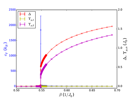
Figure 1: The specific heat, $\Delta$, and helicity moduli $\Upsilon_{\mu,i}$ for $L=64$ for $\omega=-2$. The specific heat features a $\delta$-function anomaly, characteristic of a first-order phase transition. $\Delta$ has an onset at the same value that the specific heat anomaly is found. The helicity modulus of the condensate with the smallest density is zero for all values of $\beta$. Note also the discontinuities in the $\mathbb{Z}_{2}$ -order parameter $\Delta$, and the $\mathrm{U}(1)$ -order parameters $\Upsilon_{\mu,i}$. The origin of the first-order character of the composite $\mathbb{Z}_{2}$ $\times$ $\mathrm{U}(1)$ phase-transition is due to interaction between domain walls and vortices. Details are explained in the text.

Consider lowering the temperature from the fully symmetric phase where $\Delta=\Upsilon_{\mu,i}=0$. The $\mathbb{Z}_{2}$ -symmetry is broken at a certain temperature such that $\Delta\neq 0$, i.e. $\langle\left|\psi_{1}\right|^{2}\rangle\neq\langle\left|\psi_{2}\right|^{2}\rangle$. Thus, one component gets a reduced average density and one gets an enhanced average density. These densities determine the bare phase-stiffnesses in the problem. Thus, the component with the largest density effectively has less phase fluctuations than the other one. Furthermore, due to suppression of one of the components, the helicity modulus belonging to the dominant component becomes non-zero, while the helicity modulus belonging to the minor component can remain zero. This effect is enhanced as temperature is lowered, since $\Delta$ increases monotonically with $\beta$, thus decreasing bare phase stiffness of the minor component as $\beta$ is increased. The low-temperature phase is therefore a two-component Bose fluid where one component is in a $\mathrm{U}(1)$ -ordered phase-coherent state and the other is in a $\mathrm{U}(1)$ -disordered phase-incoherent state. The spontaneous appearance of a disparity in densities reflects a broken $\mathbb{Z}_{2}$ symmetry.

Breaking a $\mathbb{Z}_{2}$ - or $\mathrm{U}(1)$ -symmetry is usually associated with a second order phase transition, i.e. a critical point. We next discuss how the above situation instead leads to a first-order phase transition. Consider heating up the system from deep within the low-temperature phase, described in the previous paragraph, until the system approaches the vicinity of the transition to the fully symmetric phase. Formation of domain walls implies regions of suppressed density as well as imposes cutoffs to vorticity, thus enhancing phase fluctuations. On the other hand, thermally-induced vortices can decrease domain-wall tension. Thus, both the $\mathbb{Z}_{2}$ -transition and $\mathrm{U}(1)$ transitions can take place preemptively, compared to single-component models. Under such circumstances two phase transitions can merge into a single first order phase transition.

A similar mechanism for producing a single first-order phase transition by merging second-order phase transitions, has previously been discussed in different systems with competing topological excitations, such as the so-called $s+is$ superconducting states Bojesen et al. (2014), in $U(1)\times U(1)$ systems with electromagnetic and drag couplingsDahl et al. (2008); Herland et al. (2010), and as an interpretation of observed first order phase transitions in multicomponent gauge theories Kuklov et al. (2006); Kragset et al. (2006); Kuklov et al. (2005, 2004). The phenomenon therefore appears quite generic in the physics of multi-component condensates.

To corroborate the above discussion, we have performed finite size scaling of the specific heat peak height for system sizes $L\in\{24,32,40,48,56,64\}$. The scaling is shown in Fig. 2 on a logarithmic scale, and the exponent obtained is $\alpha/\nu=3.38(8)$. This is consistent with a first order transition, where the exponent would be $3$.

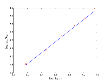
Figure 2: Log-Log plot of the finite size scaling of the height of the specific heat curves at $L\in\{24,32,48,56,64\}$. The parameters are $\omega=-2.0$, $f=0$, and $\eta=5.0$. The exponent obtained is $\alpha/\nu=3.38(8)$.

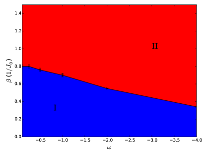
Figure 3: The phase diagram of the two-component Bose Einstein condensate at zero rotation, $f=0$, $\eta=5$, and $\omega<0$. The high-temperature phase, region I, is a two-component miscible normal fluid. The low-temperature phase, region II, is an immiscible (phase-separated) superfluid. The solid line separating these two phases is a first-order phase transition where a composite $\mathrm{U}(1)$ $\times$ $\mathbb{Z}_{2}$ -symmetry is broken.

For $L=64$, we have performed similar computations for $w=\{-0.1,-0.25,-0.5,-1,-2\}$. The results for $f=0$ are summarized in Fig. 3. The low-temperature phase is a two-component immiscible (phase-separated) superfluid with spontaneously broken $\mathbb{Z}_{2}$ -symmetry, while the high-temperature phase is a two-component miscible normal fluid. The solid line separating these two phases is a first-order phase transition where a $\mathrm{U}(1)$ - and a $\mathbb{Z}_{2}$ -symmetry are broken simultaneously. The endpoint of the phase-transition line at $\omega=0$ is a point where the system acquires an $SU(2)$-symmetry (see e.g.Galteland et al. (2015)).

IV Mixing and superfluid phase transitions in the presence of rotation

We next consider the effect of imposing a finite rotation on the condensate. Our main results are presented for a system size of $L=64$ and $f=1/32$, but we have considered system sized $L\in\{32,64,96,128\}$.

Introducing a finite amount of (rotation-induced) vortices in the ground state significantly alters the simple phase diagram presented in Fig. 3. The first effect is to suppress the parameter regime where a broken $\mathbb{Z}_{2}$ -symmetry is found, $\Delta\neq 0$. Recall that for $f=0$, any $\omega<0$ sufficed to bring about $\Delta\neq 0$ at sufficiently low $\beta$, as seen in Fig. 3. A finite amount of vortices alters this. Vortices interact via long range current-current interactions. It is energetically favorable to maximize the distance between vortices, subject to the constraint that a specific number of them has to be contained within a given area perpendicular to the direction of rotation. This effect leads to a uniform distribution of minima (equivalently maxima) in the condensate densities. On the other hand, density suppression by vortices in one component in general allows the second to nucleate. The short-range repulsive inter-component density-density interaction $(\eta-\omega)(|\psi_{1}|^{2}|\psi_{2}|^{2}+|\psi_{2}|^{2}|\psi_{1}|^{2})$ (which exceeds the intra-component density-density interaction $(\eta+\omega)(|\psi_{1}|^{2}|\psi_{1}|^{2}+|\psi_{2}|^{2}|\psi_{2}|^{2})$ for $\omega<0$), tends to produce regions where densities one component is large while the other is small, and vice versa. Below a critical value of $-\omega=-\omega_{c}\approx+0.6$, we do not see any onset of $\Delta\neq 0$ at any value of $\beta$ as the system is cooled from a uniform state. That is, the interface tension between the phases is sufficiently low and the overall free energy, which includes long range inter vortex interaction is minimized by the state with $\Delta=0$.

For the subsequent discussion, it helps to consider a schematic phase diagram of the system with $f\neq 0$, which we have obtained through large-scale Monte-Carlo simulations. The phase diagram is shown in Fig. 4. Region I denotes the simple translationally invariant high-temperature $\mathbb{Z}_{2}$ - and $\mathrm{U}(1)$ $\times$ $\mathrm{U}(1)$ -symmetric two-component phase with equal densities of both condensate components. Region II shows the $\mathbb{Z}_{2}$ -symmetric striped phase. Region III is a region with broken $\mathbb{Z}_{2}$ -symmetry, with one stiff condensate component in a uniform hexagonal vortex lattice phase, and one component in a uniform vortex liquid phase. Region IV is a region with broken $\mathbb{Z}_{2}$ -symmetry, but with the two condensates both in a vortex-liquid phase. Thus, the phase transition separating region I from region II is a phase-transition line separating a two-component isotropic vortex liquid from a two-component striped (nematic) vortex liquid. The line separating region I from Region IV is one where a $\mathbb{Z}_{2}$ -symmetry is broken, and the line separating region II from region IV is one where a translational symmetry is broken and the system acquires non-zero helicity modulus

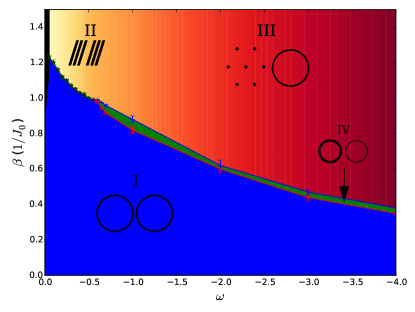
Figure 4: The phase diagram of the two-component Bose Einstein condensate at finite rotation, $f\neq 0$, $\eta=5$, and $\omega<0$. Negative $\omega$ may lead to the breaking of the $\mathbb{Z}_{2}$ -symmetry in the problem, in addition to the usual breaking of the obvious $\mathrm{U}(1)$ $\times$ $\mathrm{U}(1)$ - symmetry. Region I is a $\mathbb{Z}_{2}$ - as well as $\mathrm{U}(1)$ $\times$ $\mathrm{U}(1)$ -symmetric two-component vortex-liquid phase. Region II is a $\mathbb{Z}_{2}$ -symmetric striped (nematic) phase consisting of a two-component vortex liquid with broken translational symmetry in a direction perpendicular to the stripes, but not in the direction parallel to the stripes. Region III is a phase with broken $\mathbb{Z}_{2}$ -symmetry, and with broken translational symmetry in one condensate component, but not the other. Region IV is similar to Region III, except that no translational symmetry is broken in either condensate component. Details are explained in the main body of the paper.

IV.1 Transition from region I to region II

We first consider the thermally driven transition from the high-temperature symmetric two-component vortex liquid phase, region I, to the low-temperature two-component striped (nematic) phase, region II, for fixed negative $\omega$, but where $|\omega|<|\omega_{c}|$, i.e. to the left of the splitting point where Region IV opens up.

In Fig. 5 we show the specific heat $c_{V}$, helicity moduli in the $z$-direction $\Upsilon_{z,i}$ as the inverse temperature $\beta$ is varied, for $f=1/32$ and $\omega=-0.50$. This corresponds to a value of $-\omega$ to the left of the splitting point where Region IV opens up (see Fig. 4). The longitudinal helicity moduli $\Upsilon_{z,i}$ of both components develop a finite expectation value. The onset of this finite value is accompanied by an anomaly in the specific heat.

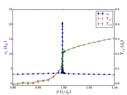
Figure 5: Specific heat, $c_{V}$, and helicity moduli along the $z$-axis ,$\Upsilon_{z,i}$, with $f=1/32$ and $\omega=-0.50$, i.e as the system transitions from Region I to Region II in Fig. 4.

We note the sharp, $\delta$-function anomaly in the specific heat and the discontinuous behavior of the helicity moduli in both components. These features are all straightforwardly interpreted as signals of a first-order phase transition. This is furthermore borne out by performing a computation of the histogram of the free energy versus internal energy of the system at precisely at the transition, see Fig. 6. This shows a double-dip structure with a peak in between, the standard hallmark of two degenerate coexisting states separated by a surface whose energy is given by the height of the peak between the minima. This surface energy clearly scales up with system size (more precisely it scales with the cross-sectional area of the system), while the difference between the energies separating the two degenerate states approaches as finite value as system size increases. The histograms develop into two separate $\delta$-function peaks as the system size increases, while the difference in the internal energy between the two degenerate states of equal probability (equivalently of equal free energy) is the latent heat of the system. The latter clearly approaches a finite value per degree of freedom as the system size increases, demonstrating the first-order character of the transition.

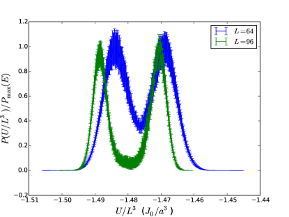
Figure 6: Histograms of the probability distribution of the internal energy per site, $U/L^{3}$, at the transition point $\omega=-0.5,\beta\approx 0.9995$, separating Region I from Region II in Fig. 4, for $L=\{64,96\}$. multi-histogram reweighting was used to obtain histograms with approximately equal peak heights.

To further characterize the transition I $\rightarrow$ II, Fig. 7, shows the $\mathbb{Z}_{2}$ order parameter $\Delta$ and the structure functions $S_{i}({\bf q}_{\perp}),i\in(1,2)$ in a narrow range around the transition point. From the top panel, it is seen that $\Delta=0$ for all $\beta$ considered. Moreover, we see that as $\beta$ is increased, the structure function evaluated at a ${\bf q}$-vectors, ${\bf G}_{c}\equiv(\pm\pi/32,\pm\pi/32)$ on the Bragg-circle of the vortex-liquids are reduced, while the structure function evaluated at Bragg peaks, ${\bf G}_{s}\equiv(\pm\pi/32,\mp\pi/32)$, corresponding to a uniform striped phase of $f=1/32$ increases. The onset of the latter marks the transition from a uniform two-component vortex liquid to a two-component nematic vortex liquid, a striped phase. The mechanism for producing the striped phase is described above. Note that in the thermodynamic limit, isolated vortex sheets can be expected to be in the state of one dimensional liquid at any finite temperature in analogy with the absence of crystalline order in one dimensional systems.

We thus conclude that the transition from Region I to region II is a first order phase-transition involving the breaking of a composite $\mathrm{U}(1)$ $\times$ $\mathrm{U}(1)$ symmetry, from an isotropic two-component vortex liquid in Region I to a two-component nematic phase of intercalated lattices of stripes of one-dimensional vortex liquids in Region II. We next go on to consider in some more detail the structure functions, primarily to gain more insight into the character of the striped phase of Region II.

The four bottom panels of Fig. 7 show the structure functions $S_{i}({\bf q}_{\perp}),i\in(1,2)$ at two values of $\beta$, $\beta=0.990$ and $\beta=1.010$. At $\beta=0.990$, both structure functions show ring-like structures characteristic of an isotropic liquid. Notice also that the intensity of the rings are equal, which is a consequence of the fact that $\Delta=0$. At $\beta=1.010$, both structure functions have developed Bragg peaks in one direction bot no Bragg peaks in the corresponding perpendicular direction. This is indicative of a striped phase.

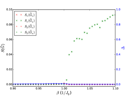
(a)

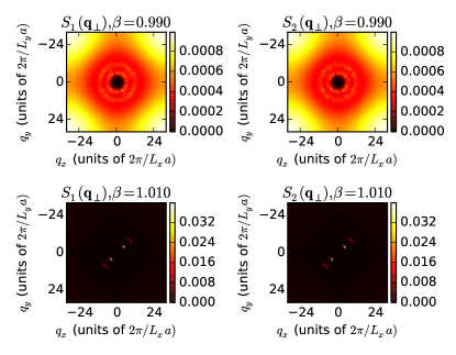
(b)

Figure 7: $\mathbb{Z}_{2}$ order parameter $\Delta$ and vortex structure functions $S_{i}({\bf q}_{\perp}),i\in(1,2)$ in the vicinity of the transition from Region I to Region II, Fig. 4, with $f=1/32,\omega=-0.50$. Panel (a) shows $\Delta$ as a function of $\beta$, as well as structure functions at specific points in reciprocal space, $S_{i}({\bf G}_{s})$ and $S_{i}({\bf G}_{c})$. The four bottom panels show the structure functions $S_{1}({\bf q}_{\perp})$ and $S_{2}({\bf q}_{\perp})$ for the two values $\beta=0.990$ and $\beta=1.010$.

This may be further corroborated by correlating the structure functions with real-space vortex structures for various values of $\beta$. This is shown in Fig. 8

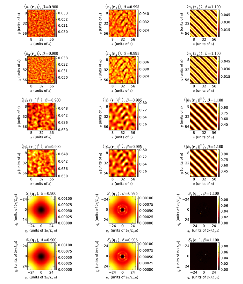
Figure 8: Tableaux showing detailed real space and reciprocal space pictures of the transition from region I to region II. The inverse temperature is varied between each column, $\beta\in\{0.900,0.995,1.100\}$. Each row show, in order, averaged vortex densities of each component, $\langle n_{i}(\mathbf{r}_{\perp})\rangle$, averaged amplitude densities of each component, $\langle\left|\psi_{i}(\mathbf{r}_{\perp})\right|\rangle$, and vortex structure functions of each component, $S_{i}({\bf q}_{\perp})$. The first column corresponds to an inverse temperature well within region I, the second column is at an inverse temperature just below where the transition into region II occurs, while the last column is well within region II.

One aspect of the structure functions shown in the two bottom rows of Fig. 8, is particularly important. Consider first the case $\beta=0.900$, well within region $1$ for $\omega<\omega_{c}$. This is shown in the first column of Fig. 8. The real-space vortex configurations in both components are disordered. Moreover, $S_{i}({\bf q}_{\perp}),i\in(1,2)$ both feature ring-structures characteristic of an isotropic liquid phase. The value of $|{\bf q}|$ at which the rings appear is a measure of the average inverse separation between the vortices in the isotropic liquids. The intensities of both structure functions is the same. Consider next the case $\beta=0.995$, shown in the second column of Fig. 8. From the real-space pictures, one discerns a tendency towards stripe-formation. This is reflected in $S_{i}({\bf q}_{\perp}),i\in(1,2)$, where the ring-like structures now instead are anisotropic, developing peaks in the direction perpendicular to the direction of the incipient stripes. At even lower temperatures $\beta=1.100$, well within region II where stripes are fully developed, the tendency towards anisotropies in $S_{i}({\bf q}_{\perp}),i\in(1,2)$ is even more obvious. This is shown in the last column of Fig. 8. In this case, Bragg-peaks have fully developed in the directions perpendicular to the stripes. There are, however, no Bragg peaks in the direction parallel to the stripes. If the stripes were perfectly straight, there would be two weak Bragg peaks in these directions. This would be the one-dimensional analog of the ring-like liquid structures of the isotropic liquid. The value of $|{\bf q}|$ at which this single weak peak occurs corresponds to the inverse average separation between vortices within the stripes. The reason they are not observed in our calculations, is due to the slight fluctuations in the shape of the stripes, which wash the Bragg peaks out.

We thus conclude that region II is a striped phase where the stripes form one-dimensional (1D) vortex liquids. Vortices in quasi-1D systems have finite energy and cannot form a 1D solid at any finite temperature. This is consistent with the structure factor we observe. On the other hand, the interaction between stripes may not be negligible, so the details of the phase diagram in Region II warrant further investigation. A notable feature of this state is the finite helicity moduli in $z$-direction, even if the structure factors show absence of vortex ordering within stripes. This highly unusual situation originates with the positive interface energy between the two condensates. That is, consider a stripe-liquid in $x$-direction. A vortex line in the $z$-direction is free to execute transverse meanderings in the $x$-direction. A superflow in the $z$-direction would produce a $y$-component of the Magnus-force on the $x$-components of the fluctuating vortex lines. However, vortex segments are restrained from moving in $y$-direction due to the stripe interface tension. This results in the observed finite helicity modulus in z-direction. Similar results are found for a number of other $\omega$-values we have considered, for $-\omega<0.6$.

IV.2 Transition from region I to region III, via region IV

Increasing $-\omega$ further, such that the inter-species density-density interaction increases, eventually favors a different pattern of phase-separation of the two components, despite the uniforming effect of long-range current-current interactions between rotation-induced vortices. This leads to a broken $\mathbb{Z}_{2}$ -symmetry. The condensate component with a globally suppressed density will therefore be in a vortex-liquid phase while the condensate component with globally enhanced density will be in a vortex lattice phase. The combined preemptive $\mathrm{U}(1)$ $\times$ $\mathbb{Z}_{2}$ phase transition found for $f=0$, now splits into two separate phase transitions. The splitting occurs because the $\mathrm{U}(1)$ -sector directly couples to the rotation, while the $\mathbb{Z}_{2}$ -sector does not. The phase-transition in the stiff $\mathrm{U}(1)$ -sector, which is a vortex-lattice melting, is therefore separated from the $\mathbb{Z}_{2}$ -transition by an amount which depends on $f$.

Since $\Delta$ increases with $-\omega$ beyond $-\omega_{c}$, the transition temperature for the $\mathbb{Z}_{2}$ -transition increases. This effectively makes the dominant component stiffer as $-\omega$ increases. Thus, the temperature for melting the vortex lattice in the dominant $\mathrm{U}(1)$ -sector also increases with increasing $-\omega$. The splitting between the $\mathrm{U}(1)$ - and the $\mathbb{Z}_{2}$ -sectors also increases as $-\omega$ increases.

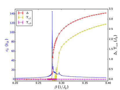
Figure 9: The phase transitions between Region I and Region IV, and between Region IV and Region III, for $f=1/32,\omega=-4.0$, and $L=128$. Note the separation between the onset of $\Delta$ and $\Upsilon_{z,i}$. The onset of $\Delta$ signals the breaking of a $\mathbb{Z}_{2}$ -symmetry, along with the associated anomaly in specific heat $C_{V}$. This marks the transition from Region I to Region IV in Fig. 4. In Region IV, we have $\Delta\neq 0$, while both components remain in isotropic vortex liquid states. In passing from Region IV to Region III in Fig. 4, the onset of one of the helicity moduli, $\Upsilon_{z,1}$ say, signals the freezing of the vortex liquid in the corresponding component, while the absence of an onset of the helicity modulus, $\Upsilon_{z,2}$ say, in the other component shows that this component remains in a vortex liquid phase. The onset of $\Upsilon_{z,1}$ signals the breaking of a $\mathrm{U}(1)$ -symmetry associated with vortex-liquid freezing.

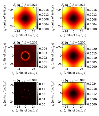
Figure 10: The phase transitions of the system for $f=1/32,\omega=-4.0$. Structure functions $S_{1}({\bf q}_{\perp})$ and $S_{2}({\bf q}_{\perp})$ at three different values of $\beta$, namely $\beta=(0.275,0.290,0.310)$, corresponding to Regions I, IV, and III in Fig. 4, respectively.

This is illustrated in Fig. 9, showing $\Delta$, specific heat $C_{V}$, and $\Upsilon_{z,1},\Upsilon_{z,2}$ as functions of $\beta$. The $\mathbb{Z}_{2}$ order parameter $\Delta$ has an onset at $\beta_{\mathbb{Z}_{2}}$, at which the specific heat has an anomaly. There is no onset of $\Upsilon_{z,1}$, showing that component $1$ remains in a vortex liquid phase. Component $2$ forms a vortex solid at lower temperature, as evidenced by the onset of $\Upsilon_{z,2}$. This happens at a $\beta_{\mathrm{U}(1)}$ which is separated from $\beta_{\mathbb{Z}_{2}}$, as explained above.

Fig. 10 shows the structure functions $S_{1}({\bf q}_{\perp})$ and $S_{2}({\bf q}_{\perp})$ at $\omega=-4.0$ at three different values of $\beta$, namely $\beta=(0.275,0.290,0.310)$. These values correspond to Regions I, IV, and III in Fig. 4, respectively. Here again, we see the freezing of one component across the transition, while the other component remains in the liquid phase. The additional information we get out of these panels is that one component remains an isotropic vortex liquid, while the other component freezes into a hexagonal vortex liquid. This sets the low-temperature Region III (see Fig. 4) at $\omega=-4.0$ drastically apart from the low-temperature Region II (see Fig. 4) at $\omega=-0.50$. The latter features a low-temperature two-component nematic vortex liquid phase with broken rotational invariance, the former case features a low-temperature mixed isotropic vortex liquid/hexagonal vortex lattice phase.

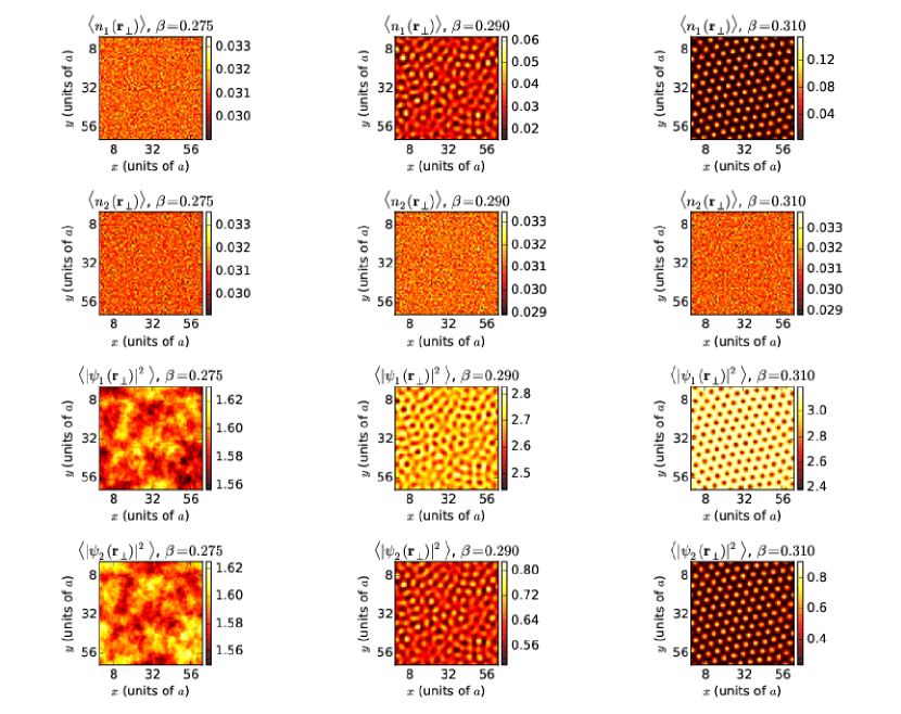
Figure 11: Tableaux showing detailed real space pictures of the transition from region I to region III, via Region IV. The inverse temperature is varied between each column, $\beta\in\{0.275,0.290,0.310\}$, and $\omega=-4$. Each row shows, from top to bottom, averaged vortex densities of each component, $\langle n_{i}(\mathbf{r}_{\perp})\rangle$, and averaged amplitude densities of each component, $\langle\left|\psi_{i}(\mathbf{r}_{\perp})\right|\rangle$. Note the vortex-ordering in one of the components, and the lack of vortex-ordering in the other component, as the system transitions from the symmetric phase region I ($\beta=0.275$) to the low-temperature phase region III ($\beta=0.310$). Note also the disparity in density-amplitudes in the two components in the intermediate regime region IV ($\beta=0.290$), due to the $\mathbb{Z}_{2}$ -symmetry breaking.

For a more detailed overview of the transition, Fig. 11 show the evolution of $\langle n_{i}(\mathbf{r}_{\perp})\rangle$, $\langle\left|\psi_{i}(\mathbf{r}_{\perp})\right|\rangle$, and $S_{i}({\bf q}_{\perp})$ across the three regions, I, IV, and III. If one follows the evolution of the vortex densities in each component, it is seen that the component which acquires a low stiffness in region IV and III is virtually unchanged, i.e. it remains in a completely uniform state. The other component, on the other hand, evolves from a uniform state in region I, through being close to freezing into a hexagonal lattice in region IV, and finally into a hexagonal structure in region III. The amplitude densities corroborate this picture. In region I they are on average equal and uniform, while in region IV the difference in stiffness is clearly seen. Here some inhomogeneities arise in the stiff component as the vortices are close to entering a hexagonal phase, which is also reflected in the soft component simply because of the local intercomponent repulsion. In region III, the amplitude density of the stiff component is high and uniform with small dips corresponding to each vortex. The soft component is low and uniform with small peaks, again due to intercomponent interactions.

IV.3 Transition from region II to region III

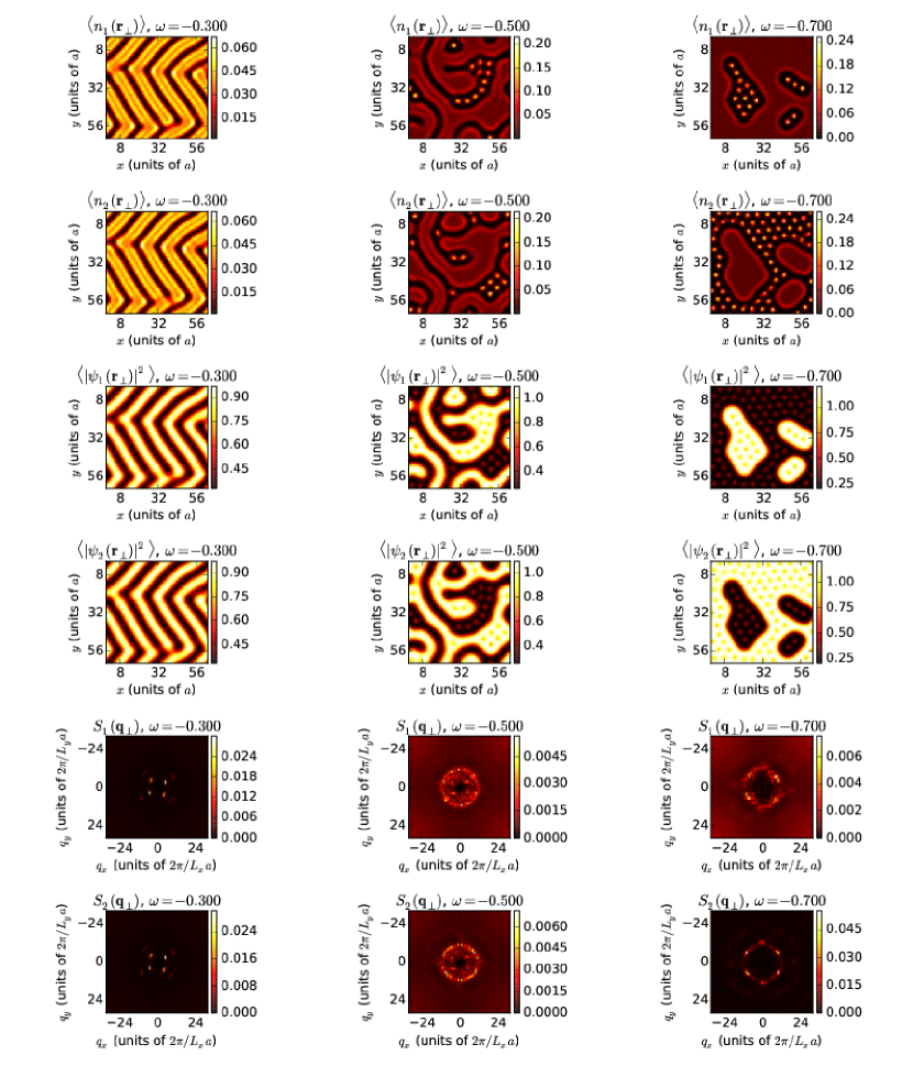
Figure 12: Tableaux showing detailed real space and reciprocal space pictures of the transition from region II to region III. The parameter $\omega$ is varied between each column, $\omega\in\{-0.300,-0.500,-0.700\}$. Each row shows, from top to bottom, averaged vortex densities of each component, $\langle n_{i}(\mathbf{r}_{\perp})\rangle$, averaged amplitude densities of each component, $\langle\left|\psi_{i}(\mathbf{r}_{\perp})\right|\rangle$, and vortex structure functions of each component, $S_{i}({\bf q}_{\perp})$. The first column shows a configuration close to region II, the second column is a configuration from the highly metastable crossover region, while the last column shows a configuration close to region III.

Finally, we consider the transition from Region II to Region III. In Region II, we have $\Delta=0$, while in Region III, $\Delta\neq 0$. Therefore the Regions II and III are separated by a $\mathbb{Z}_{2}$ -symmetry breaking. Stripe-forming systems in general have complicated structural transitions. We find an intermediate regime where the lattice of stripes has disordered, but where the hexagonal lattice/isotropic liquid-mixture has not yet fully developed. This results in multiple metastable, but robust coexisting phases of vortices in components 1 and 2 residing in different parts of the condensate. These two coexisting phases are separated by a surface of positive surface energy. This surface constrains the motion of vortex systems. As a result, in the finite systems which we simulate, the helicity moduli $\Upsilon_{z,i}$ acquire nonzero values in both components in this intermediate regime.

As $-\omega$ is increased further, such that one component becomes dominant and the other is suppressed, the minor component becomes normal. Note that when the inclusions of the normal component become isolated, they represent quasi-1D subsystems. Quasi-1D systems are superfluid only at zero temperature. However, simulations on finite systems may still display finite helicity modulus. As the density of the component increases, the corresponding intra-component current-current interaction between the rotation-induced vortices in this component increases. Hence, the intra-component long-range interaction for this component dominates, and a hexagonal vortex-lattice results. Consequently, the helicity-moduli in the two components have quite different behavior as $-\omega$ increases. In the component that eventually takes up a vortex lattice state, it increases monotonically with $-\omega$. In the other component, it is non-monotonic as a function of $\omega$, eventually approaching $0$ deep into Region III.

Typical examples of the vortex structures that appear between Region II and Region III in Fig. 4 are shown in Fig. 12. These are all metastable, long-lived states which prevent equilibration of the system. We have been unable to locate the sharp separatrix between these two regions, and whether there are other stable intermediate phases due to the lack of equilibration. Note that this problem is known in other stripe-forming systems where phases are separated by metastable and glassy states Sellin and Babaev (2013); Garaud and Babaev (2015).

V Conclusions

In this paper, we have considered the states of a two-component Bose Einstein condensate in the situation where inter-component density-density interactions dominate over the intra-component density-density interactions. The two components of the condensate are assumed to be comprised of homonuclear atoms in two different hyperfine states. The problem features an Ising-like symmetry. This Ising (or $\mathbb{Z}_{2}$ ) symmetry emerges from the dominance of the inter-component interactions over the intra-component ones. The spontaneous breaking of this Ising-symmetry corresponds to a spontaneously generated, interaction-driven, imbalance between condensates in different hyperfine states.

At finite rotation, we find four regions, denoted Regions I, II, III, and IV, of thermodynamically stable states, see Fig. 4. Region I is a high-temperature regime where the system remains in a two-component isotropic vortex liquid phase with equal densities of both components, i.e. no imbalance between condensate components in different hyperfine states. Region II is a nematic phase (broken rotational symmetry) with ordered stripes of one-dimensional vortex liquids, and with no imbalance between components of different hyperfine states. This state features a spontaneously broken composite $\mathrm{U}(1)$ $\times$ $\mathrm{U}(1)$ -symmetry, but is $\mathbb{Z}_{2}$ -symmetric. In addition it spontaneously breaks translation symmetry in one direction due to formation of periodic modulation of condensates. Region III is a mixed state with one component in a $\mathrm{U}(1)$ -symmetric isotropic vortex liquid phase while the other component resides in a hexagonal vortex lattice phase with broken $\mathrm{U}(1)$ -symmetry. The origin of the different behaviors of the two components is that Region III also features a spontaneously broken $\mathbb{Z}_{2}$ -symmetry, i.e. an imbalance between the density of one hyperfine state and the other. The component with a large density has higher phase stiffness than the component with the lower density, hence the discrepancy in their vortex states. Finally, Region IV is a region intermediate between Region I and Region III, in which $\mathrm{U}(1)$ -symmetry is not broken in either of the components, but where a spontaneously generated imbalance between densities of hyperfine states exists. Both components are in an isotropic and disordered vortex state.

The phase transition from Region I to Region II in Fig. 4 is a first-order composite $\mathrm{U}(1)$ $\times$ $\mathrm{U}(1)$ transition. The phase transition between Region I and Region IV is associated with a spontaneous $\mathbb{Z}_{2}$ symmetry breaking where a density-imbalance between condensates of different hyperfine states sets in. The phase-transition between Region IV and Region III is a first order $\mathrm{U}(1)$ transition associated with the freezing of an isotropic vortex liquid in one component into a hexagonal vortex lattice in the same component, while the other component (the one with depleted density due to the $\mathbb{Z}_{2}$ -symmetry breaking) remains in the isotropic vortex liquid phase. The phase transition from Region II to Region III, driven by increasing the dominance of inter-component density-density interactions over intra-component density-density interactions, involves at the very least a spontaneous breaking of a $\mathbb{Z}_{2}$ -symmetry as the two condensate components pass from a nematic state of intercalated lattices of one dimensional vortex liquids into a mixed state of an isotropic vortex liquid in one component and a hexagonal vortex lattice in the other component. Other than that, this transition is characterized by a broad regime of metastable states with inhomogeneous phase separation.

Fig. 11 suggests that the rotation frequency is much smaller than the second critical frequency $\Omega_{c2}$. A very rough esitimate, based on core size, gives $\Omega\propto 0.1\Omega_{c2}$. This puts the system well outside the regime of lowest-Landau level physics. The system is therefore indeed in a regime where it makes sense to talk about vortex-degrees of freedom rather than zeroes of the order parameter as the relevant degrees of freedom. For this rotation frequency, we have found the critical value of $\omega$ (one of our interaction parameters) to observe phase IV to be $\omega_{c}\approx-0.6$. From this, we find from Eq. 7 that this requires scattering lengths $a_{12}/a_{11}>1.3$. Since these scattering lengths a priori are very similar, and can be manipulated with Feshbach resonances, it seems feasible to be able to observe phase IV. In order to see the striped ground states phase II, the requirement is only that $a_{12}/a_{11}>1$, which certainly seems to be within the realms of possibility.