Interpretable Aircraft Engine Diagnostic via Expert Indicator Aggregation

Abstract

Detecting early signs of failures (anomalies) in complex systems is one of the main goal of preventive maintenance. It allows in particular to avoid actual failures by (re)scheduling maintenance operations in a way that optimizes maintenance costs. Aircraft engine health monitoring is one representative example of a field in which anomaly detection is crucial. Manufacturers collect large amount of engine related data during flights which are used, among other applications, to detect anomalies. This article introduces and studies a generic methodology that allows one to build automatic early signs of anomaly detection in a way that builds upon human expertise and that remains understandable by human operators who make the final maintenance decision. The main idea of the method is to generate a very large number of binary indicators based on parametric anomaly scores designed by experts, complemented by simple aggregations of those scores. A feature selection method is used to keep only the most discriminant indicators which are used as inputs of a Naive Bayes classifier. This give an interpretable classifier based on interpretable anomaly detectors whose parameters have been optimized indirectly by the selection process. The proposed methodology is evaluated on simulated data designed to reproduce some of the anomaly types observed in real world engines.

Keywords:

Engine Health Monitoring; Turbofan; Fusion; Anomaly Detection.

1 Introduction

Automatic anomaly detection is a major issue in numerous areas and has generated a vast scientific literature [5]. We focus in this paper on a very important application case, aircraft engine health monitoring which aims at detecting early signs of failures, among other applications [1, 18]. Aircraft engines are generally made extremely reliable by their conception process and thus have low rate of operational events. For example, in 2013, the CFM56-7B engine, produced jointly by Snecma and GE aviation, has a rate of in flight shut down (IFSD) of $0.002$ (per 1000 Engine Flight Hour) and a rate of aborted take-off (ATO) of $0.005$ (per 1000 departures). This dispatch availability of nearly 100 % (99.962 % in 2013) is obtained via regular maintenance operations but also via engine health monitoring (see also e.g. [19] for an external evaluation).

This monitoring is based, among other sources, on data transmitted by satellites between aircraft and ground stations. Typical transmitted messages include engine status overview as well as useful measurements collected as specific instants (e.g., during engine start). Flight after flight, measurements sent are analyzed in order to detect anomalies that are early signs of degradation. Potential anomalies can be automatically detected by algorithms designed by experts. If an anomaly is confirmed by a human operator, a maintenance recommendation is sent to the company operating the engine.

As a consequence, unscheduled inspections of the engine are sometimes required. These inspections are due to the abnormal measurements. Missing a detection of early signs of degradation can result in an IFSD, an ATO or a delay and cancellation (D&C). Despite the rarity of such events, companies need to avoid them to minimize unexpected expenses and customers’ disturbance. Even in cases where an unscheduled inspection does not prevent the availability of the aircraft, it has an attached cost: it is therefore important to avoid as much as possible useless inspections.

We describe in this paper a general methodology to built complex automated decision support algorithms in a way that is comprehensible by human operators who take final decisions. The main idea of our approach is to leverage expert knowledge in order to build hundreds of simple binary indicators that are all signs of the possible existence of an early sign of anomaly in engine health monitoring data. The most discriminative indicators are selected by a standard forward feature selection algorithm. Then an automatic classifier is built on those features. While the classifier decision is taken using a complex decision rule, the interpretability of the features, their expert based nature and their limited number allows the human operator to at least partially understand how the decision is made. It is a requirement to have a trustworthy decision for the operator. It should be noted that while this paper focuses on aircraft engines, the methodology can be applied to various other contexts. For instance a related but simpler methodology was proposed in [10] in the context of malware detection.

The rest of the paper is organized as follows. Section 2 describes the engine health monitoring context. The methodology is presented in details in Section 3. Section 4 is dedicated to a simulation study that validates the proposed approach.

2 Application context

2.1 Flight data

Engine health monitoring is based in part on flight data acquisition. Engines are equipped with multiple sensors which measure different physical quantities such as the high pressure core speed (N2), the Fuel Metering Valve (FMV), the Exhausted Gas Temperature (EGT), etc. (See Figure 1.) Those measures are monitored in real time during the flight. For instance the quantities mentioned before (N2, FMV, etc.) are analyzed, among others, during the engine starting sequence. This allows one to check the good health of the engine. If a potential anomaly is detected, a diagnostic is sent to an operator of the owner of the engine. The airline may then have to postpone the flight or cancel it, depending on the criticality of the fault and the estimated repair time.

Figure 1: Localization of some followed parameters on the Engine

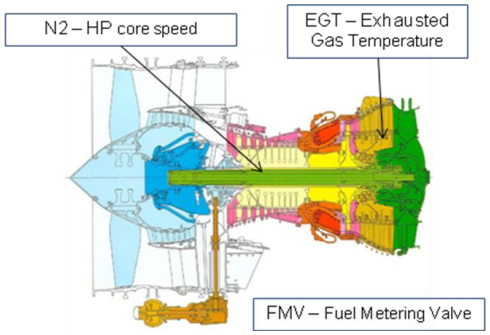
The monitoring can also be done flight after flight to detect any change that can be flagged as early signs of degraded behavior. This is done by compressing the in flight measurements into engine status overviews. The methodology introduced in this article is mostly designed for this latter kind of monitoring.

2.2 Detecting faults and abnormal behaviors

Traditional engine health monitoring is strongly based on expert knowledge and field experience (see e.g. [1, 18] for surveys and [7] for a concrete example). Faults and early signs of faults are identified from suitable measurements associated to adapted computational transformation of the data. For instance, the different measurements (temperatures, vibration, etc.) are influenced by the flight parameters (e.g. throttle position) and conditions (outside temperature, etc.). Variations in the measured values can therefore result from variations in the parameters and conditions rather than being due to abnormal behavior. Thus a typical computational transformation consists in preprocessing the measurements in order to remove dependency to the flight context [15].

In practice, the choice of measurements and computational transformations is generally done based on expert knowledge. For instance in [17], a software is designed to record expert decision about a time interval on which to monitor the evolution of such a measurement (or a time instant when such a measurement should be recorded). Based on the recorded examples, the software calibrates a pattern recognition model that can automatically reproduce the time segmentation done by the expert. Once the indicators have been computed, the normal behavior of the indicators can be learned. The residuals between predictions and actual indicators can be statistically modeled as a Gaussian vector, for instance. A score measurement is obtained from the likelihood of this distribution. The normalized vector is a failure score signature that may be described easily by experts to identify the fault origin, in particular because the original indicators have some meaning for them. See [6], [7] and [14] for other examples.

However experts are generally specialized on particular subsystems, thus each algorithm focuses mainly on a specific subsystem despite the need of a diagnostic of the whole system.

2.3 Data and detection fusion

The global diagnostic is currently done by the operator who collects all available results of diagnostic applications. The task of taking a decision based on all incoming information originating from different subsystems is difficult. A first difficulty comes from dependencies between subsystems which means that for instance in some situations, a global early sign of failure could be detected by discovering discrepancies between seemingly perfectly normal subsystems. In addition, subsystem algorithms can provide conflicting results or decisions with very low confidence levels. Furthermore, the extreme reliabilities of engines lead to an exacerbated trade off between false alarm levels and detection levels, leading in general to a rather high level of false alarms, at least at the operator level. Finally, the role of the operator is not only to identify a possible early sign of failure, but also to issue recommendations on the type of preventive maintenance needed. In other words, the operator needs to identify the possible cause of the potential failure.

2.4 Objectives

The long term goal of engine health monitoring is to reach automated accurate, trustworthy and precise maintenance decisions during optimally scheduled shop visits, but also to drastically reduce operational events such as IFSD and ATO. However, partly because of the current industrial standard, pure black box modeling is unacceptable. Indeed, operators are currently trained to understand expertly designed indicators and to take complex integrated decisions on their own. In order for a new methodology to be accepted by operators, it has at least to be of a gray box nature, that is to be (partially) explainable via logical and/or probabilistic reasoning. Then, our objective is to design a monitoring methodology that helps the human operator by proposing integrated decisions based on expertly designed indicators with a “proof of decision”.

3 Architecture of the Decision Process

3.1 Engine health monitoring data

In order to present the proposed methodology, we first describe the data obtained via engine health monitoring and the associated decision problem.

We focus here on ground based long term engine health monitoring. Each flight produces dozens of timestamped flight events and data. Concatenating those data produces a multivariate temporal description of an engine whose dimensions are heterogeneous. In addition, sampling rates of individual dimensions might be different, depending on the sensors, the number of critical time points recorded in a flight for said sensor, etc.

Based on expert knowledge, this complex set of time series is turned into a very high dimensional indicator vector. The main idea, outlined in the previous section, is that experts generally know what is the expected behavior of a subsystem of the engine during each phase of the flight. Then the dissimilarity between the expected behavior and the observed one can be quantified leading to one (or several) anomaly scores. Such scores are in turn transformed into binary indicators where $1$ means an anomaly is detected and $0$ means no anomaly detected. This is somewhat related to the way malware are characterized in [10], but with a more direct interpretation of each binary feature.

This transformation has two major advantages: it homogenizes the data and it introduces simple but informative features (each indicator is associated to a precise interpretation related to expert knowledge). It leads also to a loss of information as the raw data are in general not recoverable from the indicators. This is considered here a minor inconvenience as long as the indicators capture all possible failure modes. This will be partially guaranteed by including numerous variants of each indicator (as explained below). On a longer term, our approach has to be coupled with field experience feedback and expert validation of its coverage.

After the expert guided transformation, the monitoring problem becomes a rather standard classification problem: based on the binary indicators, the decision algorithm has to decide whether there is an anomaly in the engine and if, this is the case, to identify the type of the anomaly (for instance by identifying the subsystem responsible for the potential problem).

We describe now in more details the construction of the binary indicators.

3.2 Some types of anomalies

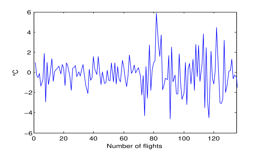
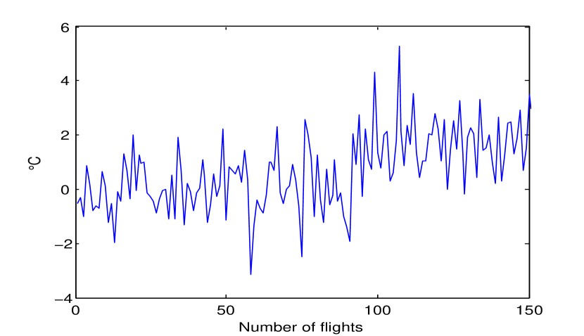
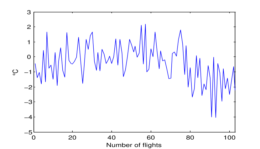
Some typical univariate early signs of anomalies are shown on Figures 4, 4 and 4 which display the evolution through time of a numerical value extracted from real world data. One can identify, with some practice, a variance shift on Figure 4, a mean shift on Figure 4 and a trend modification (change of slope) on Figure 4. In the three cases, the change instant is roughly at the center of the time window.

Figure 2: Variance shift

Figure 3: Mean shift

Figure 4: Trend modification

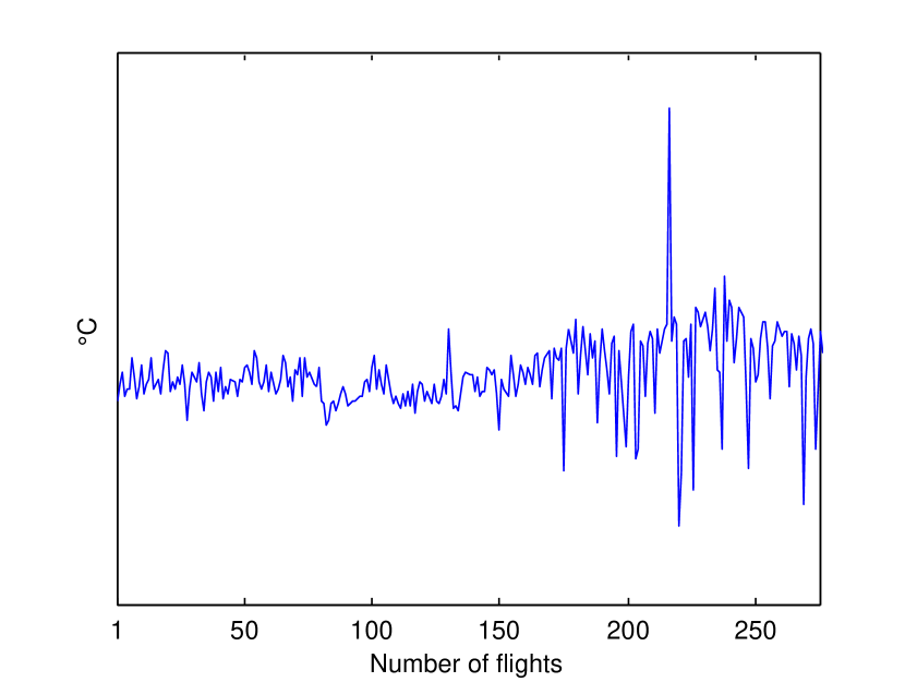
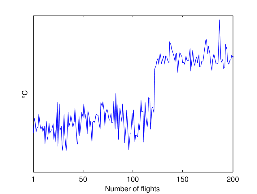
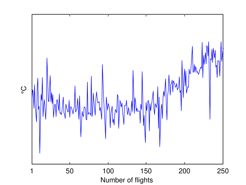
The main assumption used by experts in typical situations is that, when external sources of change have been accounted for, the residual signal should be stationary in a statistical sense. Assuming that a signal of length $m$

$$X_{i}=(X_{i1}(\theta_{1}),...,X_{im}(\theta_{m})),$$

is made of $m$ values generated independently from a fixed parametric probability model with a parameter $\theta$. In this framework, the signal is stationary if the parameters are fixed, that is, if all the $\theta_{j}$ are identical. Then, detecting an anomaly amounts to detecting a change in the time series (as illustrated by the three Figures above). This can be done via numerous techniques [5] in particular with well known statistical tests [2]. In the multivariate cases, similar shifts in the signal can be associated to anomalies. More complex scenarios, involving for instance time delays, can also be designed by experts.

3.3 Exploring the parameter space

While experts can generally describe explicitly what type of change they are expecting for some specific early signs of anomaly, they can seldom provide detailed parameter settings for statistical tests (or even for the aggregation technique that could lead to a statistical test after complex calculations). To maximize coverage it seems natural to include numerous indicators based on variations of the anomaly detectors compatible with expert knowledge.

Let us consider for illustration purpose that the expert recommends to look for shifts in mean of a certain quantity as early signs of a specific anomaly. If the expert believes the quantity to be normally distributed with a fixed variance, then a natural test would be Student’s t-test. If the expert has no strong priors on the distribution, a natural test would be the Mann–Whitney U test. Both can be included to maximize coverage.

Then, in both cases, one has to assess the time scale of the shift. Indeed those tests work by comparing summary statistics of two populations, before and after a possible change point. To define the populations, the expert has to specify the length of the time windows to consider before and after the possible change point: this is the expected time scale at which the shift will appear. In most cases, the experts can only give a rough idea of the scale. Again, maximizing the coverage leads to the inclusion of several scales compatible with the experts’ recommendations.

Given the choice of the test, of its scale and of a change point, one can construct a statistic. A possible choice for the indicator could be the value of the statistic or the associated $p$-value. However, we choose to use simpler indicators to ease their interpretation. Indeed, the raw value of a statistic is generally difficult to interpret. A $p$-value is easier to understand because of the uniform scale, but can still lead to misinterpretation by operators with insufficient statistical training. We therefore choose to use binary indicators for which the value 1 corresponds to a rejection of the null hypothesis of the underlying test to a given level (the null hypothesis is here the case with no mean shift).

3.4 Confirmatory indicators

Finally, as pointed out before, aircraft engines are extremely reliable, a fact that increases the difficulty in balancing sensibility and specificity of anomaly detectors. In order to alleviate this difficulty, we build high level indicators from low level tests. For instance, if we monitor the evolution of a quantity on a long period compared to the expected time scale of anomalies, we can compare the number of times the null hypothesis of a test has been rejected on the long period with the number of times it was not rejected, and turn this into a binary indicator with a majority rule.

3.5 Decision

To summarize, we construct parametric anomaly scores from expert knowledge, together with acceptable parameter ranges. By exploring those ranges, we generate numerous (possible hundreds of) binary indicators. Each indicator can be linked to an expertly designed score with a specific set of parameters and thus is supposedly easy to interpret by operators. Notice that while we are focused in this presentation on temporal data, this framework can be applied to any data source.

The final decision step consists in classifying these high dimensional binary vectors into at least two classes, i.e., the presence or absence of an anomaly. A classification into more classes is highly desirable if possible, for instance to further discriminate between seriousness of anomalies and/or sources (in terms of subsystems of the engine).

As explained before, we aim in the long term at gray box modeling, so while numerous classification algorithms are available see e.g. [13], we shall focus on interpretable ones. In this paper, we choose to use Random Forests [3] as they are very adapted to binary indicators and to high dimensional data. They are also known to be robust and to provide state-of-the-art classification performances at a very small computational cost. While they are not as interpretable as their ancestors CART [4], they provide at least variable importance measures that can be used to identify the most important indicators.

Another classification algorithms used in this paper is naive Bayes classifier [12] which is also appropriate for high dimensional data. They are known to provide good results despite the strong assumption of the independence of features given the class. In addition, decisions taken by a naive Bayes classifier are very easy to understand thanks to the estimation of the conditional probabilities of the feature in each class. Those quantities can be shown to the human operator as references.

Finally, while including hundreds of indicators is important to give a broad coverage of the parameter spaces of the expert scores and thus to maximize the probability of detecting anomalies, it seems obvious that some redundancy will appear. Unlike [10] who choose features by random projection, the proposed methodology favors interpretable solutions, even at the expense of the classification accuracy: the goal is to help the human operator, not to replace her/him. Therefore, we have chosen to apply a feature selection technique [9] to this problem. The reduction of number of features will ease the interpretation by limiting the quantity of information transmitted to the operators in case of a detection by the classifier. Among the possible solutions, we choose to use the Mutual information based technique Minimum Redundancy Maximum Relevance (mRMR, [16]) which was reported to give excellent results on high dimensional data (see also [8] for another possible choice).

4 A simulation study

4.1 Introduction

It is difficult to find real data with early signs of degradations, because their are scarce and moreover the scheduled maintenance operations tend to remove these early signs. Experts could study in detail recorded data to find early signs of anomalies whose origins were fixed during maintenance but it is close to looking for a needle in a haystack, especially considering the huge amount of data to analyze. We will therefore rely in this paper on simulated data. Our goal is to validate the interest of the proposed methodology in order to justify investing in the production of carefully labelled real world data.

In this section we begin by the description of the simulated data used for the evaluation of the methodology, and then we will present the performance obtained on this data.

4.2 Simulated data

The simulated data are generated according to the univariate shift models described in Section 3.2: each observation $X_{i}$ is a short time series which is recorded as at specific time points, e.g., $X_{i}=(X_{i}(t_{ij}))_{1\leq j\leq m_{i}}$. As pointed out in Section 3.1, signals can have different time resolutions. This difficulty is integrated in the simulated data by using different lengths/dimensions for each observation (hence the $m_{i}$ numbers of time points). Notice that the time points $(t_{ij})_{1\leq j\leq m_{i}}$ are introduced here only for generative purposes and are not used in the actual decision process. For multivariate data sets, they could become useful (e.g. to correlate potential shift detection), but this is out of the scope of the present paper.

In the rest of the paper, the notation $Z\sim\mathcal{N}(\mu,\sigma^{2})$ says that the random variable $Z$ follows a Gaussian distribution with mean $\mu$ and variance $\sigma^{2}$ and the notation $W\sim\mathcal{U}(S)$ says that the random variable $W$ follows the uniform distribution on the set $S$ (which can be finite such as $\{1,2,3\}$ or infinite such as $[0,1]$).

We generate two data sets: a simple one $A$ and a slightly more complex one $B$. In both cases, it is assumed that expert based normalisation has been performed. Therefore when no shift in the data distribution occurs, we observe a stationary random noise modeled by the standard Gaussian distribution. This assumption made about the noise may seem very strong but the actual goal of this paper is to evaluate the methodology and we choose to use simple distribution and simple statistical tests. In the future, we plan to use more realistic noise associated with more complex tests. An observation $X_{i}$ with no shift is then generated as follows:

1. $m_{i}$, the length of the signal, is chosen as $m_{i}\sim\mathcal{U}(\{100,101,\ldots,200\})$ ;

2. the $m_{i}$ values $(X_{i}(t_{ij}))_{1\leq j\leq m_{i}}$ are sampled independently from the standard Gaussian distribution, that is $X_{i}(t_{ij})\sim\mathcal{N}(\mu=0,\sigma^{2}=1)$.

Anomalous signals use the same distribution of the signal length as normal signals. More precisely, an anomalous observation $X_{i}$ is generated as follows:

1. $m_{i}$, the length of the signal, is chosen as $m_{i}\sim\mathcal{U}(\{100,101,\ldots,200\})$ ;

2. the change point $t^{s}_{i}$ is chosen as

   $$t_{i}^{s}\sim\mathcal{U}\left(\left\{\left\lfloor\frac{2m_{i}}{10}\right\rfloor,\left\lfloor\frac{2m_{i}}{10}\right\rfloor+1,\ldots,\left\lfloor\frac{8m_{i}}{10}\right\rfloor\right\}\right),$$

   where $\lfloor x\rfloor$ is the integer part of $x$. For instance, if $m_{i}=100$, then the change point is chosen among the time points $t_{20}$ to $t_{80}$ ;

3. the $m_{i}$ values $(X_{i}(t_{ij}))_{1\leq j\leq m_{i}}$ are generated according to one anomaly model.

Anomalies are in turn modelled after the three examples given in Figures 4, 4 and 4. The three types of shift are:

1. a variance shift: in this case, the parameter of the shift is the variance after the change point, $\sigma^{2}_{i}$, with $\sigma_{i}\sim\mathcal{U}([1.01,5])$. Given $\sigma_{i}$, the $(X_{i}(t_{ij}))_{1\leq j\leq m_{i}}$ are sampled independently as $X_{i}(t_{ij})\sim\mathcal{N}(\mu=0,\sigma^{2}=1)$ when $t_{ij}<t^{s}_{i}$ (before the change point) and $X_{i}(t_{ij})\sim\mathcal{N}(\mu=0,\sigma^{2}=\sigma_{i}^{2})$ when $t_{ij}\geq t^{s}_{i}$ (after the change point). See Figure 7 for an example;

2. a mean shift: in this case, the parameter of the shift is the mean after the change point, $\mu_{i}$. In set $A$, $\mu_{i}\sim\mathcal{U}([1.01,5])$ while in set $B$, $\mu_{i}\sim\mathcal{U}([0.505,2.5])$. Given $\mu_{i}$, the $(X_{i}(t_{ij}))_{1\leq j\leq m_{i}}$ are sampled independently as $X_{i}(t_{ij})\sim\mathcal{N}(\mu=0,\sigma^{2}=1)$ when $t_{ij}<t^{s}_{i}$ (before the change point) and $X_{i}(t_{ij})\sim\mathcal{N}(\mu=\mu_{i},\sigma^{2}=1)$ when $t_{ij}\geq t^{s}_{i}$ (after the change point). See Figure 7 for an example;

3. a slope shift: in this final case, the parameter of the shift is a slope $\lambda_{i}$ with $\lambda_{i}\sim\mathcal{U}([0.02,3])$. Given $\lambda_{i}$, the $(X_{i}(t_{ij}))_{1\leq j\leq m_{i}}$ are sampled independently as $X_{i}(t_{ij})\sim\mathcal{N}(\mu=0,\sigma^{2}=1)$ when $t_{ij}<t^{s}_{i}$ (before the change point) and $X_{i}(t_{ij})\sim\mathcal{N}(\mu=\lambda_{i}(t_{ij}-t^{s}_{i}),\sigma^{2}=1)$ when $t_{ij}\geq t^{s}_{i}$ (after the change point). See Figure 7 for an example.

We generate according to this procedure two data sets with 6000 observations corresponding to 3000 observations with no anomaly, and 1000 observations for each of the three types of anomalies. The only difference between data set $A$ and data set $B$ is the amplitude of the mean shift which is smaller in $B$, making the classification harder.

Figure 5: variance shift

Figure 6: mean shift

Figure 7: trend modification

4.3 Indicators

As explained in Section 3.3, binary indicators are constructed from expert knowledge by varying parameters, including scale and position parameters. In the present context, we use sliding and jumping windows: for each possible position of the window, a classical statistical test is conducted to decide whether a shift in the signal occurs at the center of the window (see Figure 8). Individual tests obtained from different positions are combined to create binary indicators.

Figure 8: Illustration of the sliding and jumping windows. $\tau$ is the length of the window. $\delta$ is the jump parameter. $t_{i}^{s}$ is the change point.

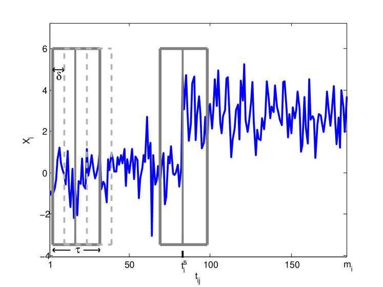
More precisely, a window of length $\tau$ is a series of $\tau$ consecutive time points in a signal $(X_{i}(t_{ij}))_{1\leq j\leq m_{i}}$ (in other words, this is a sub-signal). For a fixed $\tau\leq m_{i}$, there are $m_{i}-\tau+1$ windows in $X_{i}$, from $(X_{i}(t_{ij}))_{1\leq j\leq\tau}$ to $(X_{i}(t_{ij}))_{m_{i}-\tau+1\leq j\leq m_{i}}$ (when sorted in order of their first time points).

Given a window of length $\tau$ (assumed even) starting at position $k$, a two sample test is conducted on the two subsets of values corresponding to the first half of the window and to the second half. More precisely, we extract from the series of values $(X_{i}(t_{ij}))_{k\leq j\leq k+\tau-1}$ a first sample $S^{1}=(X_{i}(t_{ij}))_{k\leq j\leq k+\tau/2-1}$ and a second sample $S^{2}=(X_{i}(t_{ij}))_{k+\tau/2\leq j\leq k+\tau-1}$. Then a test of inequality between $S^{1}$ and $S^{2}$ is conducted (inequality is defined with respect to some statistical aspect). The “expert” designed tests are here (notice that those tests do not include a slope shift test):

1. the Mann-Whitney-Wilcoxon U test (non parametric test for shift in mean);

2. the two sample Kolmogorov-Smirnov test (non parametric test for differences in distributions);

3. the F-test for equality of variance (parametric test based on a Gaussian hypothesis).

From this general principle, we derive a large set of indicators by varying the length of the window, the level of significance of the test and the way to combine results from all the windows that can be extracted from a signal.

In practice, for an observation $(X_{i}(t_{ij}))_{1\leq j\leq m_{i}}$, we use three different window lengths, $\tau=30$, $\tau=50$ and $\tau=100$. We use also three different levels for the tests, namely 0.005, 0.1 and 0.5. For a fixed window length $\tau$ and a fixed test, an observation $(X_{i}(t_{ij}))_{1\leq j\leq m_{i}}$ is transformed into $m_{i}-\tau+1$ $p$-values produced by applying the test to the $m_{i}-\tau+1$ windows extracted from the observation. For each significance level, the $p$-values are binarized giving 1 or 0 whether the null hypothesis of identical distribution between $S^{1}$ and $S^{2}$ is rejected or not, leading to $m_{i}-\tau+1$ binary values.

The next step consists in turning the raw binary values into a set of indicators producing the same number of indicators for all observations. The simplest binary indicator equals to 1 if and only if at least one binary value among the $m_{i}-\tau+1$ is equal to 1 (that is if at least one window defines two sub-samples that differ according to the chosen test). Notice that as we use 3 window lengths, 3 tests, and 3 levels, we obtained this way 27 simple binary indicators.

Then, more complex binary indicators are generated, as explained in Section 3.4. In a way, this corresponds to build very simple binary classifiers on the binary values obtained from the tests. All those indicators are based on the notion of consecutive windows. In order to vary the time resolution of this process, we first introduce a jump parameter $\delta$. Two windows are consecutive according to $\delta$ if the first time point of the second window is the $(\delta+1)$-th time point of the first window. For instance, if $\delta=5$, $(X_{i}(t_{ij}))_{1\leq j\leq\tau}$ and $(X_{i}(t_{ij}))_{6\leq j\leq\tau+5}$ are consecutive windows. In practice, we use three values for $\delta$, namely 1, 5 and 10.

For each value of $\delta$ and for each series of $m_{i}-\tau+1$ binary values, we compute the following derived indicator:

1. the global ratio indicator is equal to 1 if and only if on a fraction of at least $\beta$ of all possible windows, the test detects a change. This indicator does not use the fact that windows are consecutive, but it is nevertheless affected by $\delta$. Indeed, values strictly larger than 1 for $\delta$ reduce the total number of windows under consideration;

2. the consecutive ratio indicator is equal to 1 if and only if there is a series of $\beta(m_{i}-\tau+1)$ consecutive windows on which the test detects a change ;

3. the local ratio indicators is equal to 1 if and only if there is a series of $l$ consecutive windows among which the tests detects at least $k$ times a change.

Those derived indicators are parametric. In the present experiments, we use three different values for $\beta$ (used by the first two derived indicators), namely 0.1, 0.3 and 0.5. For the pair $(l,k)$ used by the last derived indicator, we used three different pairs $(3,2)$, $(5,3)$ and $(5,4)$.

A simple series of $m_{i}-\tau+1$ binary values allows us to construct 27 derived indicators (3 values for $\delta$ times $3$ values for the parameters of each of the 3 types of derived indicators). As we have 27 of such series (because of the 3 window lengths, 3 tests and 3 levels), we end up with 729 additional indicators for a total of 756 binary indicators.

In addition, based on expert recommendation, we apply the entire processing both to the original signal and to a smoothed signal (using a simple moving average over 5 measurements). The total number of indicators is therefore 1512. However many of them are identical over the 6000 observations and the final number of distinct binary indicators is 810. The redundancy is explained by several aspects. For instance, while the smoothing changes the signal, it has a limited effect on the test results. Also, when the level of the test is high, the base binary values tend to be all equal to one. When the ratio $\beta$ is low, there are not many differences between the derived indicators with respect to $\delta$, etc.

It should be noted that the parameters used both for the simulated data and the indicators have been chosen so as to illustrate the possibilities of the proposed architecture of the decision process. The values have been considered reasonable (see Table 1 for a summary of these values) and representative of what would be useful in practice by experts of our application domain. It is however expected than more statistical tests and more indicators should be considered in practice to cover the range of the possible anomalies.

Parameters	Values
statistical test	Mann-Whitney-Wilcoxon U test
	Two sample Kolmogorov-Smirnov test
	F-test
length of window ($\tau$)	30
	50
	100
levels	0.005
	0.1
	0.5
jump ($\delta$)	1
	5
	10
fraction for global ratio indicator and consecutive ratio indicator ($\beta$)	0.1
	0.3
	0.5
k among l for local ratio indicators ($l,k$)	(3,2)
	(5,3)
	(5,4)
moving average	1
	5

Table 1: Listing of the values used for the parameters of the indicators.

4.4 Performance analysis

Each data set is split in a balanced way into a learning set with 1000 signals and a test set with 5000 signals (the class proportions from the full data set are kept in the subsets). We report the global classification accuracy (the classification accuracy is the percentage of correct predictions, regardless of the class) on the learning set to monitor possible over fitting. The performances of the methodology are evaluated on 10 balanced subsets of size 500 from the 5000 signals’ test set. This allows to evaluate both the average performances and their variability. For the Random Forest, we also report the out-of-bag (oob) estimate of the classification accuracy: this quantity is obtained during the bootstrap procedure used to construct the forest. Indeed each observation appears as a training observation in only roughly two third of the trees that constitute the forest. Then the prediction of the remaining trees for this observation can be aggregated to give a decision. Comparing this decision to the true value gives the out-of-bag estimate of the classification error for this observation (see [3] for details). Finally, for the Naive Bayes classifier, we use confusion matrices and class specific accuracies to gain more insights on the results when needed.

4.5 Performances with all indicators

As indicators are expertly designed and should cover the useful parameter range of the tests, it is assumed that the best classification performances should be obtained when using all of them, up to the effects of the curse of dimensionality.

Data set	Training set acc.	OOB acc.	Test set average acc.
$A$	0.9770	0.9228	0.9352 (0.0100)
$B$	0.9709	0.9118	0.9226 (0.0108)

Table 2: Classification accuracy of the Random Forest using the 810 binary indicators. For the test set, we report the average classification accuracy and its standard deviation between parenthesis.

Table 2 reports the global classification accuracy of the Random Forest, using all the indicators. As expected, Random Forests suffer neither from the curse of dimensionality nor from strong over fitting (the test set performances are close to the learning set ones). Table 3 reports the same performance indicator for the Naive Bayes classifier. Those performances are significantly lower than the one obtained by the Random Forest. As shown by the confusion matrix on Table 4, the classification errors are not concentrated on one class (even if the errors are not perfectly balanced). This tends to confirm that the indicators are adequate to the task (this was already obvious from the Random Forest).

Data set	Training set accuracy	Test set average accuracy
$A$	0.7856	0.7718 (0.0173)
$B$	0.7545	0.7381 (0.0178)

Table 3: Classification accuracy of the Naive Bayes classifier using the 810 binary indicators. For the test set, we report the average classification accuracy and its standard deviation between parenthesis.

		Predicted class
		No anomaly	Variance	Mean	Slope	total
True class	No anomaly	1759	667	45	29	2500
	Variance	64	712	50	3	829
	Mean	7	2	783	37	829
	Slope	32	7	195	595	829

Table 4: Data set $A$: confusion matrix with all indicators for Naive Bayes classifier on the full test set.

4.6 Feature selection

While the Random Forest gives very satisfactory results, it would be unacceptable for human operators as it operates in a black box way. While the indicators have simple interpretation, it would be unrealistic to ask to an operator to review 810 binary values to understand why the classifier favors one class over the others. In addition, the performances of the Naive Bayes classifier are significantly lower than those of the Random Forest one. Both drawbacks favor the use of a feature selection procedure.

As explained in Section 3.5, the feature selection relies on the mRMR ranking procedure. A forward approach is used to evaluate how many indicators are needed to achieve acceptable predictive performances. Notice that in the forward approach, indicators are added in the order given by mRMR and then never removed. As mRMR takes into account redundancy between the indicators, this should not be a major issue. Then for each number of indicators, a Random Forest and a Naive Bayes classifier are constructed and evaluated.

Figure 9: Data set $A$ Random Forest: classification accuracy on learning set (circle) as a function of the number of indicators. A boxplot gives the classification accuracies on the test subsets, summarized by its median (black dot inside a white circle). The estimation of those accuracies by the out-of-bag (oob) bootstrap estimate is shown by the crosses.

Figure 10: Data set $B$ Random Forest, see Figure 9 for details.

Figure 11: Data set $A$ Naive Bayes classifier: classification accuracy on learning set (circle) as a function of the number of indicators. A boxplot gives the classification accuracies on the test subsets, summarized by its median (black dot inside a white circle).

Figure 12: Data set $B$ Naive Bayes classifier, see Figure 11 for details.

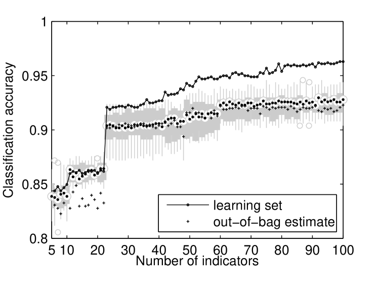
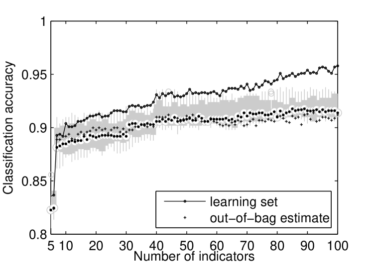
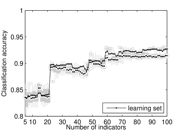
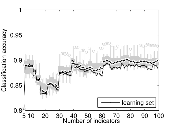
Figures 9, 10, 11 and 12 summarize the results for the 100 first indicators. The classification accuracy of the Random Forest increases almost monotonously with the number of indicators, but after roughly 25 to 30 indicators (depending on the data set), performances on the test set tend to stagnate (this is also the case of the out-of-bag estimate of the performances, which shows, as expected, that the number of indicators could be selected using this measure). In practice, this means that the proposed procedure can be used to select the relevant indicators implementing this way an automatic tuning procedure for the parameters of the expertly designed scores.

Results for the Naive Bayes classifier are slightly more complex in the case of the second data set, but they confirm that indicator selection is possible. Moreover, reducing the number of indicators has here a very positive effect on the classification accuracy of the Naive Bayes classifier which reaches almost as good performances as the Random Forest. Notice that the learning set performances of the Naive Bayes classifier are almost identical to its test set performances (which exhibit almost no variability over the slices of the full test set). This is natural because the classifier is based on the estimation of the probability of observing a 1 value independently for each indicator, conditionally on the class. The learning set contains at least 250 observations for each class, leading to a very accurate estimation of those probabilities and thus to very stable decisions. In practice one can therefore select the optimal number of indicators using the learning set performances, without the need of a cross-validation procedure (optimality is with respect to the classification accuracy).

Figure 13: Data set $A$ Naive Bayes classifier: classification error for each class on the training set (solid lines) and on the test set (dotted lines, average accuracies only).

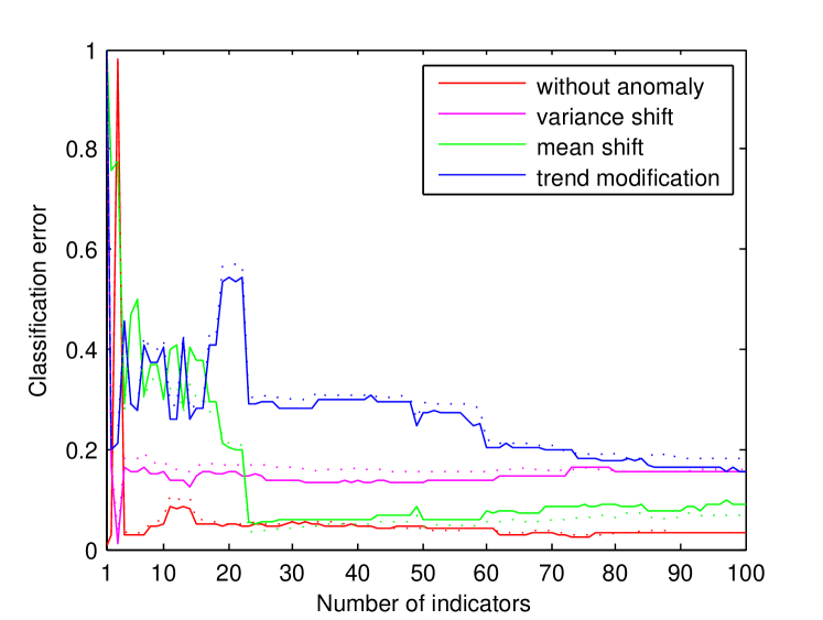
It should be noted that significant jumps in performances can be observed in all cases. This might be an indication that the ordering provided by the mRMR procedure is not optimal. A possible solution to reach better indicator subsets would be to use a wrapper approach, leveraging the computational efficiency of both Random Forest and Naive Bayes construction. Meanwhile Figure 13 shows in more detail this phenomenon by displaying the classification error class by class, as a function of the number of indicators, in the case of data set $A$. The figure shows the difficulty of discerning between mean shift and trend shift (for the latter, no specific test have been included, on purpose). But as the strong decrease in classification error when the 23-th indicator is added concerns both classes (mean shift and trend shift), the ordering provided by mRMR could be questioned.

4.7 Indicator selection

Based on results shown on Figures 11 and 12, one can select an optimal number of binary indicators, that is the number of indicators that maximizes the classification accuracy on the learning set. However, this leads in general to a too large number of indicators. Thus we restrict the search below a maximal number of indicators in order to avoid flooding the human operator with to many results.

For instance Table 5 gives the classification accuracy of the Naive Bayes classifier using the optimal number of binary indicators between 1 and 30.

Data set	Training set acc.	Test set average acc.	# of indicators
$A$	0.8958	0.8911 (0.0125)	23
$B$	0.8828	0.8809 (0.0130)	11

Table 5: Classification accuracy of the Naive Bayesian network using the optimal number binary indicators between 1 and 30. For the test set, we report the average classification accuracy and its standard deviation between parenthesis.

While the performances are not as good as the ones of the Random Forest, they are much improved compared to the ones reported in Table 3. In addition, the selected indicators can be shown to the human operator together with the estimated probabilities of getting a positive result from each indicator, conditionally on each class, shown on Table 6. For instance here the first selected indicator, $confu(2,3)$, is a confirmation indicator for the U test. It is positive when there are 2 windows out of 3 consecutive ones on which a U test was positive. The Naive Bayes classifier uses the estimated probabilities to reach a decision: here the indicator is very unlikely to be positive if there is no change or if the change is a variance shift. On the contrary, it is very likely to be positive when there is a mean or a trend shift. While the table does not “explain” the decisions made by the Naive Bayes classifier, it gives easily interpretable hints to the human operator.

type of indicator	no change	variance	mean	trend
confu(2,3)	0.010333	0.011	0.971	0.939
F test	0.020667	0.83	0.742	0.779
U test	0.027333	0.03	0.977	0.952
ratef(0.1)	0.0016667	0.69	0.518	0.221
confu(4,5)	0.034333	0.03	0.986	0.959
confu(3,5)	0.0013333	0.001	0.923	0.899
U test	0.02	0.022	0.968	0.941
F test	0.042	0.853	0.793	0.813
rateu(0.1)	0.00033333	0.001	0.906	0.896
confu(4,5)	0.019	0.02	0.946	0.927
conff(3,5)	0.052333	0.721	0.54	0.121
U test	0.037667	0.038	0.983	0.951
KS test	0.016	0.294	0.972	0.936
confu(3,5)	0.049	0.043	0.988	0.963
F test	0.030667	0.841	0.77	0.801
U test	0.043	0.043	0.981	0.963
lseqf(0.3)	0.0093333	0.749	0.59	0.36
rateu(0.1)	0.001	0.002	0.896	0.895
lsequ(0.1)	0.062667	0.06	0.992	0.949
confu(3,5)	0.025667	0.021	0.963	0.936
lseqf(0.3)	0.008	0.732	0.656	0.695
KS test	0.016333	0.088	0.955	0.93
confu(3,5)	0	0	0.003	0.673

Table 6: Probability of observing 1 conditionally the class, for each of the 23 best indicators according to mRMR for data set $A$. Confu(k,n) corresponds to a positive Mann–Whitney–Wilcoxon U test on k windows out of n consecutive ones. Conff(k,n) is the same thing for the F-test. Ratef($\beta$) corresponds to a positive F-test on $\beta\times m$ windows out of $m$. Lseqf($\beta$) corresponds to a positive F-test on $\beta\times m$ consecutive windows out of $m$. Lsequ($\beta$) is the same for a U test. Detailed parameters of the indicators have been omitted for brevity.

5 Conclusion and perspectives

In this paper, we have introduced a diagnostic methodology for engine health monitoring that leverages expert knowledge and automatic classification. The main idea is to build from expert knowledge parametric anomaly scores associated to range of plausible parameters. From those scores, hundreds of binary indicators are generated in a way that covers the parameter space as well as introduces simple aggregation based classifiers. This turns the diagnostic problem into a classification problem with a very high number of binary features. Using a feature selection technique, one can reduce the number of useful indicators to a humanly manageable number. This allows a human operator to understand at least partially how a decision is reached by an automatic classifier. This is favored by the choice of the indicators which are based on expert knowledge and on very simple decision rules. A very interesting byproduct of the methodology is that it can work on very different original data as long as expert decision can be modelled by a set of parametric anomaly scores. This was illustrated by working on signals of different lengths.

The methodology has been shown sound using simulated data. Using a reference high performance classifier, Random Forests, the indicator generation technique covers sufficiently the parameter space to obtain a high classification rate. Then, the feature selection mechanism (here a simple forward technique based on mRMR) leads to a reduced number of indicators (23 for one of the data set) with good predictive performances when paired with a simpler classifier, the Naive Bayes classifier. As shown in the experiments, the class conditional probabilities of obtaining a positive value for those indicators provide interesting insights on the way the Naive Bayes classifier takes a decision.

In order to justify the costs of collecting a sufficiently large real world labelled data set in our context (engine health monitoring), additional experiments are needed. In particular, multivariate data must be studied in order to simulate the case of a complex system made of numerous sub-systems. This will naturally lead to more complex anomaly models. We also observed possible limitations of the feature selection strategy used here as the performances displayed abrupt changes during the forward procedure. More computationally demanding solutions, namely wrapper ones, will be studied to confirm this point.

It is also important to notice that the classification accuracy is not the best way of evaluating the performances of a classifier in the engine health monitoring context. Firstly, engine health monitoring involves intrinsically a strong class imbalance [11]. Secondly, engine health monitoring is a cost sensitive area because of the strong impact on airline profit of an unscheduled maintenance. It is therefore important to take into account specific asymmetric misclassification cost to get a proper performance evaluation.

The Gaussian assumption made on the noise of the simulated data is a strong one. In our future work, we plan to use more realistic noise and to test the robustness of the methodology. We will evaluate if we can compensate this new complexity with the use of more complex indicators.

References

- [1] Jason Asher and Surya Aryan. A survey of health and usage monitoring system in contemporary aircraft. International Journal of Engineering and Technical Research, 1(9):34–41, 2013. ISSN: 2321-0869.
- [2] Michèle Basseville and Igor V. Nikiforov. Detection of abrupt changes: theory and application. Prentice-Hall, Inc., Englewood Cliffs, N.J., USA, 1993. ISBN: 0-13-126780-9.
- [3] Leo Breiman. Random forests. Machine Learning, 45(1):5–32, October 2001.
- [4] Leo Breiman, Jerome H Friedman, Richard A Olshen, and Charles J Stone. Classification and regression trees. Wadsworth Statistics/Probability. Chapman and Hall/CRC, 1984. ISBN: 978-0-412-04841-8.
- [5] Varun Chandola, Arindam Banerjee, and Vipin Kumar. Anomaly detection: A survey. ACM Computing Surveys, 41(3):1–58, July 2009.
- [6] Etienne Côme, Marie Cottrell, Michel Verleysen, and Jérôme Lacaille. Aircraft engine health monitoring using self-organizing maps. In Petra Perner, editor, Advances in Data Mining. Applications and Theoretical Aspects, volume 6171 of Lecture Notes in Computer Science, pages 405–417. Springer Berlin Heidelberg, 2010. ISBN: 978-3-642-14399-1.
- [7] Xavier Flandrois, Jérome Lacaille, Jean-Rémi Masse, and Alexandre Ausloos. Expertise transfer and automatic failure classification for the engine start capability system. In Proceedings of the 2009 AIAA Infotech@Aerospace (I@A) Conference, Seattle, WA, April 2009. AIAA (American Institute of Aeronautics and Astronautics).
- [8] F. Fleuret. Fast binary feature selection with conditional mutual information. Journal of Machine Learning Research, 5:1531–1555, November 2004.
- [9] Isabelle Guyon and André Elisseeff. An introduction to variable and feature selection. Journal of Machine Learning Research, 3:1157–1182, March 2003.
- [10] Jozsef Hegedus, Yoan Miche, Alexander Ilin, and Amaury Lendasse. Methodology for behavioral-based malware analysis and detection using random projections and k-nearest neighbors classifiers. In Proceedings of the Seventh International Conference on Computational Intelligence and Security (CIS 2011), pages 1016–1023, Hainan, China, December 2011. IEEE Computer Society. ISBN: 978-1-4577-2008-6.
- [11] Nathalie Japkowicz and Shaju Stephen. The class imbalance problem: A systematic study. Intelligent data analysis, 6(5):429–449, October 2002.
- [12] Daphne Koller and Nir Friedman. Probabilistic graphical models: principles and techniques. The MIT Press, July 2009. ISBN: 978-0-262-01319-2.
- [13] Sotiris B. Kotsiantis. Supervised machine learning: A review of classification techniques. Informatica, 31(3), 2007.
- [14] Jérôme Lacaille. A maturation environment to develop and manage health monitoring algorithms. In Proceedinds of the Annual Conference of the Prognostics and Health Management Society, San Diego, CA, September 2009. phmsociety.
- [15] Jérôme Lacaille. Standardized failure signature for a turbofan engine. In Proceedings of IEEE Aerospace conference, Big Sky, MT, Mars 2009. IEEE.
- [16] Hanchuan Peng, Fuhui Long, and Chris Ding. Feature selection based on mutual information criteria of max-dependency, max-relevance, and min-redundancy. IEEE Transactions on Pattern Analysis and Machine Intelligence, 27(8):1226–1238, August 2005.
- [17] Tsirizo Rabenoro and Jérome Lacaille. Instants extraction for aircraft engine monitoring. In Proceedings of the AIAA Infotech@Aerospace (I@A) Conference, Boston, MA, August 2013. AIAA (American Institute of Aeronautics and Astronautics).
- [18] Irem Y. Tumer and Anupa Bajwa. A survey of aircraft engine health monitoring systems. In Proceedings of 35th AIAA/ASME/SAE/ASEE Joint Propulsion Conference and Exhibit, Los Angeles, California, USA, June 1999.
- [19] Ljubiša Vasov and Branimir Stojiljković. Reliability levels estimation of JT8D-9 and CFM56-3 turbojet engines. FME Transactions, 35(1):41–45, 2007.