Non-holonomic constraints and their impact on discretizations of Klein-Gordon lattice dynamical models

Abstract.

We explore a new type of discretizations of lattice dynamical models of the Klein-Gordon type relevant to the existence and long-term mobility of nonlinear waves. The discretization is based on non-holonomic constraints and is shown to retrieve the “proper” continuum limit of the model. Such discretizations are useful in exactly preserving a discrete analogue of the momentum. It is also shown that for generic initial data, the momentum and energy conservation laws cannot be achieved concurrently. Finally, direct numerical simulations illustrate that our models yield considerably higher mobility of strongly nonlinear solutions than the well-known “standard” discretizations, even in the case of highly discrete systems when the coupling between the adjacent nodes is weak. Thus, our approach is better suited for cases where an accurate description of mobility for nonlinear traveling waves is important.

Panayotis G. Kevrekidis

Department of Mathematics and Statistics

University of Massachusetts

Amherst, MA 01003-4515, USA

Vakhtang Putkaradze

Department of Mathematics and Statistics, University of Alberta

Edmonton, Alberta, CA

Zoi Rapti

Department of Mathematics, University of Illinois at Urbana-Champaign

Urbana, Illinois 61801-2975, USA

1. Introduction

Discrete solitons such as kinks and breathers exist in many physical systems, including Josephson juctions, electrical circuits, and granular crystals [1, 2, 3]. In the models that describe these systems, the mobility of soliton solutions, and specifically kinks – which will be the focus of the present work–, is an important and well-studied property [4, 5]. For instance, kinks in extemely discrete systems need to overcome the celebrated Peierls-Nabarro barrier, while they undergo energy radiation which leads to their trapping in the lattice [9]. More recent work revealed the existence of kinks that do not experience the action of the Peierls-Nabarro potential [10].

For a class of Klein-Gordon discretizations [5] it has been shown that energy and linear momentum cannot be both conserved. This is problematic in cases when the objective is the discretization of the continuum version of equation, which conserves both momentum and energy. Going beyond the properties of isolated kinks, the above result has consequences for the studies of soliton collisions in Klein-Gordon lattices. In general, the mobility of kinks in discrete manifestations of the Klein-Gordon equation may vary from that in the continuous version as well as among different discretizations.

In this work, we present a class of discretizations based on a non-holonomic constraint that preserve the momentum and alleviate the problem of decreased mobility in kink solutions. Specifically, as we enforce the conservation of momentum it in turn implies an affine constraint in kink velocities, which is of the non-holonomic type. The extra term added in the discretization due to the non-holonomic constraint, vanishes in the continuum limit, hence demonstrating that the discretized version of the equation converges to its continuous counterpart. Our numerical results validate our theoretical considerations and we present multiple instances where the additional constraint that we impose increases the mobility of the kinks.

We shall note that for generalized non-holonomic constraints that are not linear in velocities, one has to be careful in applying the variational principle. This was demonstrated in, for example, [6, 7] for the case of stabilizing servomechanisms, where an alternative formulation through Poisson structures has been derived. The discrete equivalent of a conservation law for continuous system (1) below, enforced by the constraint, cannot be readily interpreted as a consequence of a continuous symmetry through a Noether theorem. Thus, applications of alternative methods of non-holonomic mechanics [8], in addition to the Lagrange-d’Alembert’s principle developed here, are of particular interest and will be considered in future work.

This article is structured as follows. In section 2 we describe the Klein-Gordon model that will be studied and present the theoretical framework of our method. In section 3 we present numerical results that corroborate our theoretical predictions. Finally, in section 4 we discuss our findings and offer insight for future directions.

2. Model Theoretical Setup and Proposed Discretizations

The models that we will consider herein will involve discretizations of continuum partial differential equations of the nonlinear wave type:

$$u_{tt}=u_{xx}-V^{\prime}(u).$$ (1)

There are numerous key model examples of this class of equations, such as the sine-Gordon [1] or the $\phi^{4}$ model arising from classical field theory and high-energy physics [2], as well as variants thereof.

The corresponding discrete models are of considerable interest in their own right as models of coupled torsion pendula, dislocation dynamics, Josephson junctions, electrical circuits, among numerous other settings [1, 2, 11, 12]. The generic discrete analogue of these models is derived by using a standard lattice discetization of the second space derivative as follows:

$$\ddot{u}_{n}=\epsilon(u_{n+1}+u_{n-1}-2u_{n})-V^{\prime}(u_{n})$$ (2)

The field is defined at the integer nodes $n$ and $\epsilon$ denotes the coupling constant between adjacent sites, which could be interpreted as $\epsilon=1/dx^{2}$, with $dx$ being the spacing between the adjacent sites (see below).

Note that lattice model (2) is Hamiltonian with

$$H=\sum_{n}{\frac{1}{2}\dot{u}_{n}^{2}+}\frac{{\epsilon}}{2}\left(u_{n+1}-u_{n}\right)^{2}+V(u_{n})\equiv\sum_{n}{\mathcal{H}}_{n},$$ (3)

where ${\mathcal{H}}_{n}$ is the energy density.

In that context, an alternative limit, namely $\epsilon=0$, the so-called anti-continuum limit becomes particularly important and provides a valuable tool for assessing the potential stationary or time-periodic states of the model and their respective spectral stability properties [13, 14, 15].

One of the “pathologies” of such discrete models is that as the coupling parameter $\epsilon$ decreases, the mobility of the nonlinear waves accordingly weakens [4]. The decreased mobility stems, to a considerable degree, from the fact that the momentum $P=\int u_{t}u_{x}dx$ is no longer a conservation law in the discrete case of Eq. (2), even though it is in the corresponding continuum limit of $\epsilon\rightarrow\infty$. This curious fact has spurred a considerable volume of recent work (for a partial summary, see [16]) focused on providing alternative discretizations that would enable higher mobility of the waves, even at small $\epsilon$. Our aim in the present work is to propose a novel class of such discretizations, based upon the imposition of a non-holonomic constraint providing an exact conservation of the discrete momentum.

Indeed, the continuum equation (1) provides a conservation of the momentum quantity $P_{c}=\int u_{t}u_{x}\mbox{d}x$. On the other hand, after defining the analogue of discrete momentum for (2) as

$$P=\sum\dot{u}_{n}(u_{n+1}-u_{n-1})$$ (4)

a quick check shows that such discrete momentum is not conserved [17]. The goal of this paper is to enforce the conservation of (4) using the methods of non-holonomic mechanics. The equation (2) can be obtained as the Euler-Lagrange equation with the Lagrangian

$$L=\sum\frac{1}{2}\dot{u}_{n}^{2}-\left(\frac{\epsilon}{2}(u_{n+1}-u_{n})^{2}+V(u_{n})\right)\,.$$ (5)

through the critical action principle $\delta\int L\mbox{d}t=0$ on arbitrary variations $\delta u_{n}(t)$ with appropriately vanishing boundary conditions at the end time points. Next, enforcing the conservation law (4) leads to an affine constraint in velocities of the type

$$\sum_{n}a_{n}(\mathbf{u})\dot{u}_{n}=b(\mathbf{u})\qquad{\rm with}\qquad a_{n}(\mathbf{u})=u_{n+1}-u_{n-1}\,,\,\quad b(\mathbf{u})=P$$ (6)

using the notation $\mathbf{u}=(u_{1},u_{2},\ldots,u_{n})$. Since this constraint involves velocities in a non-trivial way, i.e., that constraint cannot be integrated to contain coordinates only, the constraint is non-holonomic, and linear in velocities. The usual way of dealing with this type of constraints is through the Lagrange-d’Alembert’s principle [18]. For the constraints of the type (6), the variations $\delta u_{n}$ are no longer arbitrary, but must satisfy the linear relations

$$\sum_{n}a_{n}(\mathbf{u})\delta u_{n}=\sum_{n}\left(u_{n+1}-u_{n-1}\right)\delta u_{n}=0\,.$$ (7)

Notice that we do not enforce (6) directly, as this would correspond to the so-called vakonomic approach, relevant for e.g. the control theory but normally not leading to correct expressions for mechanical systems, as described in [19]. On the contrary, Lagrange-d’Alembert’s approach (7) was consistently shown to be physically appropriate. For more in-depth discussion of various approaches to non-holonomic systems, we refer the reader to [18, 19].

If $r$ is the Largange multiplier enforcing the constraint (7), the critical action principle coupled with the constraint gives

$$\int_{t_{0}}^{t_{1}}\left[\frac{d}{dt}\frac{\partial L}{\partial\dot{u}_{n}}-\epsilon\left(u_{n+1}+u_{n-1}-2u_{n}\right)+V^{\prime}(u_{n})-r\left(u_{n+1}-u_{n-1}\right)\right]\delta u_{n}=0\,,$$

provided $\delta u_{n}$ vanish at $t=t_{0,1}$ so no boundary integration terms appear in the equations. Since $\delta u_{n}$ is arbitrary, the equations of motion conserving momentum are

$$\ddot{u}_{n}=\epsilon\left(u_{n+1}+u_{n-1}-2u_{n}\right)-V^{\prime}(u_{n})+r(u_{n+1}-u_{n-1})\,.$$ (8)

Note the new term proportional to $r$ and enforcing the constraint on the right hand side of (8), as compared to (2). The physical meaning of $r$ is the (generalized) constraint force. In order to find $r$, we compute the derivative $dP/dt=0$ and set it equal to zero. We find that while the terms associated with $\epsilon$ vanish telescopically [17], the nonlinear term does not. This leads to the explicit condition for $r$ as

$$r=\frac{\sum_{n}V^{\prime}(u_{n})\left(u_{n+1}-u_{n-1}\right)}{\sum_{n}\left(u_{n+1}-u_{n-1}\right)^{2}}$$ (9)

Making this selection for $r$, multiplying both sides of Eq. (8) by $\dot{u}_{n}$, and summing, we observe that the derivative of the (former) Hamiltonian of Eq. (3) is not zero anymore, but is given by the following condition:

$$\frac{dH}{dt}=rP.$$ (10)

Importantly, this identity suggests that for generic initial data, such that $P\neq 0$, the Hamiltonian will not be conserved. This is due to the constraint (6) being non-homogeneous in velocities for $P\neq 0$. It is relevant to point out that such an “incompatibility” of the momentum and energy conservation laws for other broad classes of discretizations of the Klein-Gordon dynamical lattices have also been reported previously [5].

An additional comment about this non-holonomic discretization is that the extra term introduced by the non-holonomic constraint vanishes at the continuum limit $\epsilon\rightarrow\infty$, ensuring that Eq. (8) converges to the proper continuum limit of Eq. (1). To see this, we consider the continuum analogue of the new $r(u_{n+1}-u_{n-1})$ term, which is $u_{x}(\int V^{\prime}(u)u_{x}dx/\int u_{x}^{2}dx$). The numerator of the term in the parenthesis can be integrated to yield $V(u_{2})-V(u_{1})$ where $u_{2}$ and $u_{1}$ are, respectively the asymptotic values of the field at $\pm\infty$. Assuming that we examine the dynamics of homoclinic orbit or of a heteroclinic orbit in a symmetric double well (as is typically the case in the examples of interest mentioned above), this quantity vanishes identically and the discretization reverts to its proper continuum limit. We will return to this point and corroborate it through our numerical computations below. A final remark about the nature of our discretization procedure, different from all other schemes that we are aware of, is that our method is inherently nonlocal since the computation of $r$ in (9) entails a summation over the entire lattice.

3. Numerical Computations

To provide a comparison between the properties of the different discretizations, we examine the dynamics of Eq. (2) vs. that of Eq. (8). We use an initial condition in the form of a prototypical nonlinear excitation such as the kink. In the continuum limit, the latter stationary solution (which can be boosted to any sub-luminal speed via Lorentz transformation) is of the form $u(x)=\tanh(x)$. This is the case for the $\phi^{4}$ model with a potential $V(u)=(1/2)(u^{2}-1)^{2}$. For the discrete system, we have used the initial condition $u_{n}(0)=\tanh(x)=\tanh(n\times dx)$, where $dx$ is used to signal the spatial discretization step (see also below), approximating the continuous solution on a discrete set of points. Furthermore, Eqs . (2) and (8) are integrated using a fourth-order Runge-Kutta scheme with a temporal discretization step of the typical size $dt=0.00025$.

In addition, we enforce an initial momentum of $P_{fix}=0.5$ via the definition of Eq. (4). The simplest way that we envisioned for achieving this was to assume all sites as having vanishing velocity except for the central one of the chain, say $n_{0}$, and then using $\dot{u}_{n_{0}}=P_{fix}/(u_{n_{0}+1}-u_{n_{0}-1})$. This prescription provides the given amount of momentum to the central portion of the kink and we expect that it should set the kink in motion.

This is exactly what we observe in Fig. 1, which is close to the continuum limit of $\epsilon=1/dx^{2}\rightarrow\infty$. Here, as usual $dx$ is effectively the corresponding spacing between the lattice sites, leading as a finite-difference three-point approximation to the second derivative. In particular, in this figure $dx=1/4$ or $\epsilon=16$ is used. The top left panel illustrates the traveling kink of the standard discretization of Eq. (2). The proximity of the model to its continuum analogue coupled with the imparting of momentum via the initial condition leads the kink to travel through the chain with an apparently constant speed (evident in the constant slope of the two contour plots of the top panel, the left one illustrating the energy density of Eq. (3) and the right one the actual field $u_{n}(t)$). Given that the model of Eq. (2) is Hamiltonian, our explicit fourth-order time integration (Runge-Kutta) scheme conserves the initial energy (of O$(1)$) up to a few parts in $10^{-14}$ verifying its conservation for all practical purposes. On the other hand, the momentum fluctuates in the third decimal digit indicating its non-preservation by the scheme; instead, it is only approximately conserved because of the proximity to the continuum limit where the continuum analogue of Eq. (4) can be shown to be preserved by Eq. (1).

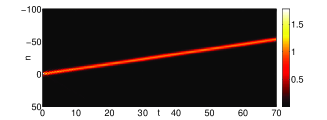
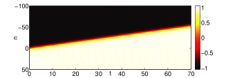
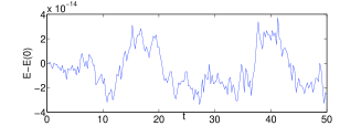
Figure 1. Evolutionary dynamics of the “standard” discrete model of Eq. (2) with $dx=1/4$, hence $\epsilon=1/dx^{2}=16$ for $V(u)=\frac{1}{2}(u^{2}-1)^{2}$ i.e., the $\phi^{4}$ model. The top left panel represents the space-time ($n-t$) contour plot of the energy density (see Eq. (3)), while the top right represents the corresponding contour of the field $u_{n}(t)$. The bottom left illustrates the “near-conservation” for this (approaching the continuum) case for the linear momentum of Eq. (4), while the bottom right illustrates that the model is energy preserving up to fluctuations of size of $10^{-14}$ due to numerical roundoff errors.

On the other hand, we can see that the fluctuations in this quantity ($P$) are far more dramatic in the considerably more discrete case $\epsilon=1$, corresponding to $dx=1$, shown on Fig. 2. There, the fluctuations in $P$ are of O$(1)$ while the energy is still conserved with the same precision as before. In addition, the motion of the kink is fundamentally different, featuring a jerky back and forth trajectory between a few sites around the origin. Thus, in this case, the kink appears trapped due to the weak inter-site coupling which does not allow the momentum to translate itself into mobility as it would in the corresponding continuum limit.

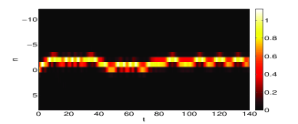
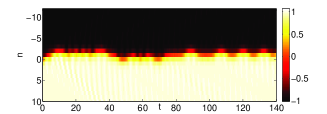
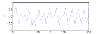
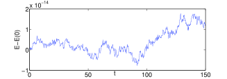
Figure 2. Same as the previous plot, only now we consider a highly discrete case $dx=\epsilon=1$. Here, we observe the detrimental effect of the energy-conserving discretization with regards to the mobility of the kink initial condition. The strong discreteness/weak coupling precludes the kink from moving through the lattice and the initial momentum (which as can be seen is far from being conserved now) is expended in a jerky motion with a range of a few discrete sites (trapping of the kink).

We now turn to the corresponding dynamics of the newly proposed model of the form of Eq. (8). The case of $dx=1/4$ is again shown in Fig. 3. The fundamental difference in this case is that the momentum $P$ of Eq. (4) in the bottom left panel is conserved to a similar accuracy as the energy in the previous model, as expected by our construction. On the contrary, the energy of the bottom right panel varies at the third significant digit remaining roughly constant solely due to the proximity to the continuum limit, where the analogue of Eq. (3) is conserved for Eq. (1).

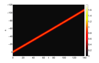
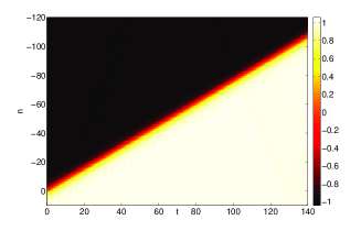
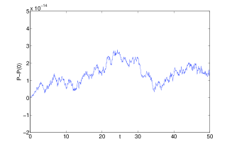
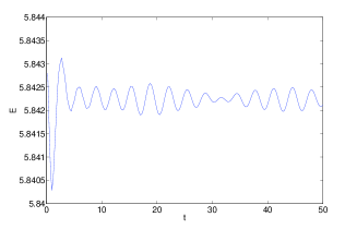
Figure 3. Same as Fig. 1 but now for the momentum conserving discretization of Eq. (8). This is the near continuum case of $dx=0.25$ which sustains motion of the kink with constant speed. The momentum of the bottom left is conserved up to numerical accuracy, while the energy of Eq. (3) in the bottom right is only approximately conserved, due to the proximity to the energy conserving continuum limit.

The main advantage of our discretization method is evident in Fig. 4. More specifically, as the example of $dx=\epsilon=1$ shown in Fig. 3 illustrates, the discretization of Eq. (8) presented here can accurately describe traveling waves in the case of strong coupling. Fig. 3 shows that the momentum preserved up to numerical accuracy, as expected, while the energy fluctuations become more significant, revealing the absence of energy conservation already in the second significant digit. It should also be mentioned that we have also separately verified Eq. (10) numerically, although we do not present it here. Hence, our principal numerical conclusion is that the models of Eq. (8) ensure a higher mobility of their corresponding coherent structures compared with the standard discretization of Eq. (2). This comes at the price of the incorporation of the nonlocal effect through the summation that ensures the conservation of the linear momentum.

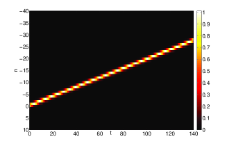
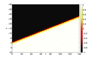
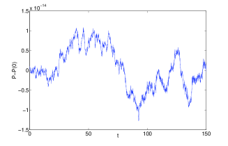
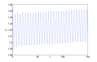
Figure 4. Same as Fig. 4 but now for $\epsilon=1$ (corresponding to $dx=1$). Notice that despite the high discreteness of the model and the weakness of the coupling, the mobility of the state is well preserved.

Lastly, we have confirmed that the relevant discretizations are indeed properly converging to the continuum limit as $dx\rightarrow 0$. A typical example of this approach is shown in Fig. 5. In particular, the figure showcases the evolution of the quantity $r(t)$, which constitutes the prefactor of the newly proposed nonlocal term arising through the non-holonomic constraint. It can be seen that as we go from the weakly-coupled strongly discrete case of the left panel (for $dx=1$) to the right panel, closer to continuum case of $dx=0.25$, the value of $r(t)$ decreases by more than an order of magnitude

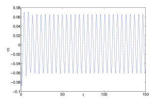
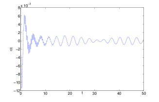
Figure 5. Corroboration of the convergence of the discrete model of Eq. (8) to the continuum limit of Eq. (1). The time evolution of the quantity $r(t)$ is shown, in the left panel for $dx=1$ and in the right for $dx=0.25$. It can be seen that the quantity assumes significantly smaller values in the latter case in comparison to the former, and indeed this trend continues for decreasing values of $dx$, with $r\rightarrow 0$, as $dx\rightarrow 0$.

4. Conclusions and Future Challenges

In the present work, we have revisited the theme of discretizations of continuum nonlinear partial differential equations of the wave type. We have focused on the example of Klein-Gordon equations and offered a novel class of schemes which can be summarized as follows: (a) they can be straightforwardly designed to conserve linear momentum; (b) when they do so, they do not in general conserve the energy, (c) they revert to the continuum PDE in the appropriate limit of the lattice spacing tending to zero; and (d) they are based on the imposition of a non-holonomic constraint and thus are fundamentally different than previously proposed schemes due to their nonlocal nature. We have argued that these models have intriguing characteristics, such as the ability to impart high mobility to localized coherent states, a feature corroborated via numerical computations in the case of kinks of the $\phi^{4}$ model. This feature is preserved even in the regime of high discreteness/weak coupling where the standard discretizations under the same initial data produce kinks that are trapped within the Peierls-Nabarro energy barrier and cannot move through the chain.

This study opens an interesting new direction for the investigation of the relevance of such schemes from a numerical perspective and also for a more detailed understanding of their properties. While in the present initial communication we have focused on the dynamics of kinks, it would be relevant to explore corresponding structural features for discrete breather type solutions [20]. Furthermore, while in the present work we have focused on the one-dimensional domains only, it would be particularly interesting to consider generalizing such models in higher dimensions. The latter have progressively become a theme of considerable attention over the past few years [21, 22] and hence it would again be particularly relevant to compare the standard higher dimensional discretizations, with the ones produced by the multi-dimensional generalization of the non-holonomic constraint concepts presented herein. Such studies are presently in progress and will be reported in future publications.

References

- [1] J. Cuevas-Maraver, P.G. Kevrekidis and F. Williams (Eds.), The sine-Gordon model and its applications: From pendula and Josephson Junctions to Gravity and High-Energy Physics, Springer-Verlag, Heidelberg, 2014.
- [2] R.K. Dodd, J.C. Eilbeck, J.D. Gibbon, and H.C. Morris, Solitons and Nonlinear Wave Equations, Academic, New York, 1983.
- [3] N. Boechler, G. Theocharis, S. Job, P. G. Kevrekidis, M. A. Porter, and C. Daraio, Discrete Breathers in One-Dimensional Diatomic Granular Crystals Phys. Rev. Lett., 104 (2010), 244302.
- [4] M. Peyrard and M.D. Kruskal, Kink dynamics in the highly discrete sine-Gordon system, Physica D, 14 (1984) 88-102.
- [5] S.V. Dmitriev, P.G. Kevrekidis, N. Yoshikawa, Standard nearest-neighbour discretizations of Klein Gordon models cannot preserve both energy and linear momentum, J. Phys. A, 39 (2006), 7217-7226.
- [6] C.-M. Marle, Rep. Math. Phys. Various approaches to conservative and nonconservative nonholonomic systems, 42 (1998) , 211-229.
- [7] H. Cendra and S. Grillo, Lagrangian systems with higher order constraints, J. Math. Phys. 47 (2006), 022902.
- [8] V. I. Arnold, V. V. Kozlov and A. I. Neistadt, Mathematical Methods of Classical and Celestial Mechanics, 3rd Ed, Springer (2006).
- [9] Y. S. Kivshar and D. K. Campbell, Peierls-Nabarro potential for highly localized nonlinear modes Phys. Rev. E , 48 (1993), 3077-3081.
- [10] S.V. Dmitriev, P.G. Kevrekidis, N. Yoshikawa, Discrete Klein Gordon models with static kinks free of the Peierls Nabarro potential, J. Phys. A, 38 (2005), 7617-7627.
- [11] M. Remoissenet, Waves called solitons, Springer-Verlag, Berlin, 1999.
- [12] T. Dauxois and M. Peyrard, Physics of Solitons, Cambridge University Press, Cambridge, 2006.
- [13] R.S. MacKay and S. Aubry, Proof of existence of breathers for time-reversible or Hamiltonian networks of weakly coupled oscillators, Nonlinearity, 7 (1994), 1623-1643.
- [14] S. Aubry, Breathers in nonlinear lattices: existence, linear stability and quantization Physica D 103 (1997), 201-250.
- [15] P.G. Kevrekidis, Non-linear waves in lattices: past, present, future, IMA J. Appl. Math., 76 (2011), 389-423.
- [16] D.E. Pelinovsky, Translationally invariant nonlinear Schr dinger lattices Nonlinearity, 19 (2006), 2695-2715.
- [17] P.G. Kevrekidis, On a class of discretizations of Hamiltonian nonlinear partial differential equations, Physica D, 183 (2003), 68-86.
- [18] A. A. Bloch, Nonholonomic Mechanics and Control, Interdisciplinary Applied Mathematics, Springer, 2009.
- [19] V. I. Arnold, V. V. Kozlov and A. I. Neishtadt, Mathematical aspects of classical and celestial mechanics, Encyclopedia of Mathematical Sciences, Springer, 2007.
- [20] S. Flach and A.V. Gorbach, Discrete breathers advances in theory and applications Phys. Rep. 467 (2008), 1-116.
- [21] L.A. Cisneros, J. Ize and A.A. Minzoni, Modulational and numerical solutions for the steady discrete Sine Gordon equation in two space dimensions, Physica D 238 (2009), 1229-1240.
- [22] J.G. Caputo and M.P. Soerensen, Radial sine-Gordon kinks as sources of fast breathers Phys. Rev. E 88 (2013), 022915.