Convergence of Structured Quadratic Forms With Application to Theoretical Performances of Adaptive Filters in Low Rank Gaussian Context

Abstract

This paper addresses the problem of deriving the asymptotic performance of adaptive Low Rank (LR) filters used in target detection embedded in a disturbance composed of a LR Gaussian noise plus a white Gaussian noise. In this context, we use the Signal to Interference to Noise Ratio (SINR) loss as performance measure which is a function of the estimated projector onto the LR noise subspace. However, although the SINR loss can be determined through Monte-Carlo simulations or real data, this process remains quite time consuming. Thus, this paper proposes to predict the SINR loss behavior in order to not depend on the data anymore and be quicker. To derive this theoretical result, previous works used a restrictive hypothesis assuming that the target is orthogonal to the LR noise. In this paper, we propose to derive this theoretical performance by relaxing this hypothesis and using Random Matrix Theory (RMT) tools. These tools will be used to present the convergences of simple quadratic forms and perform new RMT convergences of structured quadratic forms and SINR loss in the large dimensional regime, i.e. the size and the number of the data tend to infinity at the same rate. We show through simulations the interest of our approach compared to the previous works when the restrictive hypothesis is no longer verified.

I Introduction

In array processing, the covariance matrix $\mathbf{R}$ of the data is widely involved for main applications as filtering [1, 2], radar/sonar detection [3] or localization [4, 5]. However, when the disturbance in the data is composed of the sum of a Low Rank (LR) correlated noise and a White Gaussian Noise (WGN), the covariance matrix is often replaced by the projector onto the LR noise subspace $\mathbf{\Pi}_{\mathrm{c}}$ [6, 7, 8, 9]. In practice, the projector onto the LR noise subspace (and the covariance matrix) is generally unknown and an estimate is consequently required to perform the different processing. This estimation procedure is based on the so-called secondary data assumed to be independent and to share the same distribution. Then, the true projector is replaced by the estimated one in order to obtain an adaptive processing. An important issue is then to derive the theoretical performances of the adaptive processing as a function of the number of secondary data $K$. The processing based on the covariance matrix has been widely studied and led to many theoretical results in filtering [1] and detection [10, 11, 12, 13]. For example, for classical adaptive processing, $K=2m$ secondary data (where $m$ is the data size) are required to ensure good performance of the adaptive filtering, i.e. a 3dB loss of the output Signal to Interference plus Noise Ratio (SINR) compared to optimal filtering [1]. For LR processing, some results has been obtained especially in filtering [6, 14, 15, 16] and localization [17]. Similarly, in LR filtering, the number $K$ of secondary data required to ensure good performance of the adaptive filtering is equal to $2r$ (where $r$ is the rank of the LR noise subspace) [6, 14].

These last results are obtained from the theoretical study of the Signal to SINR loss. More precisely, in [14, 16], the derivation of the theoretical results is based on the hypothesis that the steering vector is orthogonal to the LR noise subspace. Nevertheless, even if the result seems to be close to the simulated one when the hypothesis is no longer valid anymore [18], it is impossible with traditional techniques of [14, 16] to obtain a theoretical performance as a function of the distance between the steering vector and the LR noise subspace. Since, in practice, this dependence is essential to predict the performance of the adaptive filtering, we propose in this paper to derive the theoretical SINR loss, for a disturbance composed of a LR noise and a WGN, as a function of $K$ and the distance between the steering vector and the LR noise subspace. The proposed approach is based on the study of the SINR loss structure.

The SINR loss (resp. LR SINR loss) is composed of a simple Quadratic Form (QF) in the numerator, $\bm{s}_{1}^{H}\hat{\mathbf{R}}^{-1}\bm{s}_{2}$ (resp. $\bm{s}_{1}^{H}\hat{\mathbf{\Pi}}^{\bot}_{\mathrm{c}}\bm{s}_{2}$) and a structured QF in the denominator $\bm{s}_{1}^{H}\hat{\mathbf{R}}^{-1}\mathbf{R}\hat{\mathbf{R}}^{-1}\bm{s}_{2}$ (resp. $\bm{s}_{1}^{H}\hat{\mathbf{\Pi}}^{\bot}_{\mathrm{c}}\mathbf{R}\hat{\mathbf{\Pi}}^{\bot}_{\mathrm{c}}\bm{s}_{2}$). These recent years, the simple QFs (numerator) have been broadly studied [19, 20, 21, 22] using Random Matrix Theory (RMT) tools contrary to structured QFs (denominator). RMT tools have also been used in array processing to improve the MUSIC algorithm [23, 24] and in matched subspace detection [25, 26] where the rank $r$ is unknown. The principle is to examine the spectral behavior of $\mathbf{\hat{R}}$ by RMT to obtain their convergences, performances and asymptotic distribution when $K$ tends to infinity and when both the data size $m$ and $K$ tend to infinity at the same ratio, i.e. $m/K\rightarrow c\in]0,+\infty)$, for different models of $\mathbf{\hat{R}}$ of the observed data as in [19, 20, 23], [22] and [21]. Therefore, inspired by these works, we propose in this paper to study the convergences of the structured QFs $\bm{s}_{1}^{H}\hat{\mathbf{R}}^{-1}\mathbf{R}\hat{\mathbf{R}}^{-1}\bm{s}_{2}$ (resp. $\bm{s}_{1}^{H}\hat{\mathbf{\Pi}}^{\bot}_{\mathrm{c}}\mathbf{R}\hat{\mathbf{\Pi}}^{\bot}_{\mathrm{c}}\bm{s}_{2}$): when 1) $K\rightarrow\infty$ with a fixed $m$ and when 2) $m,K\rightarrow\infty$ at the same ratio under the most appropriated model for our data and with the rank assumed to be known. From [27, 28], the spiked model has proved to be the more appropriated one to our knowledge. This model, introduced by [29] (also studied in [30, 31] from an eigenvector point of view) considers that the multiplicity of the eigenvalues corresponding to the signal (the LR noise for us) is fixed for all $m$ and leads to the SPIKE-MUSIC estimator [32] of $\bm{s}_{1}^{H}\bm{\hat{\Pi}}\bm{s}_{2}$. Then, the new results are validated through numerical simulations. From these new theoretical convergences, the paper derives the convergence of the SINR loss for both adaptive filters (the classical and the LR one). The new theoretical SINR losses depend on the number of secondary data $K$ but also on the distance between the steering vector and the LR noise subspace. This work is partially related to those of [33, 34] and [35] which uses the RMT tools to derive the theoretical SINR loss in a full rank context (previously defined as classical).

Finally, these theoretical SINR losses are validated in a jamming application context where the purpose is to detect a target thanks to a Uniform Linear Antenna (ULA) composed of $m$ sensors despite the presence of jamming. The response of the jamming is composed of signals similar to the target response. This problem is very similar to the well-known Space Time Adaptive Processing (STAP) introduced in [2]. Results show the interest of our approach with respect to other theoretical results [6, 14, 15, 16] in particular when the target is close to the jammer.

The paper is organized as follows. Section II presents the received data model, the adaptive filters and the corresponding SINR losses. Section III summarizes the existing studies on the simple QFs $\bm{s}_{1}^{H}\mathbf{\hat{R}}\bm{s}_{2}$ and $\bm{s}_{1}^{H}\mathbf{\hat{\Pi}}\bm{s}_{2}$, and exposes the covariance matrix model, the spiked model. Section IV gives the theoretical contribution the paper with the convergences of the structured QFs $\bm{s}_{1}^{H}\mathbf{\hat{\Pi}}_{\mathrm{c}}^{\bot}\mathbf{B}\mathbf{\hat{\Pi}}_{\mathrm{c}}^{\bot}\bm{s}_{2}$ and $\bm{s}_{1}^{H}\mathbf{\hat{\Pi}}_{\mathrm{c}}^{\bot}\mathbf{R}\mathbf{\hat{\Pi}}_{\mathrm{c}}^{\bot}\bm{s}_{2}$ and the convergences of the SINR losses. The results are finally applied on a jamming application in Section V.
Notations: The following conventions are adopted. An italic letter stands for a scalar quantity, boldface lowercase (uppercase) characters stand for vectors (matrices) and $(.)^{H}$ stands for the conjugate transpose. $\mathbf{I}_{N}$ is the $N\times N$ identity matrix, $\mathrm{tr}(.)$ denotes the trace operator and $\mathrm{diag}(.)$ denotes the diagonalization operator such as $(\mathbf{A})_{i,i}=(\mathrm{diag}(\mathbf{a}))_{i,i}=(\mathbf{a})_{i}$ and $(\mathbf{A})_{i,j}=0$ if $i\neq j$. $\#\left\{\mathcal{A}\right\}$ denotes the cardinality of the set $\mathcal{A}$. $[\![a,b]\!]$ is the set defined by $\left\{x\in\mathbb{Z}:a\leqslant x\leqslant b,\forall(a,b)\in\mathbb{Z}^{2}\right\}$. $\bm{\mathbbm{O}}_{n\times N}$ is a $n\times N$ matrix full of 0. The abbreviations iid and a.s. stem for independent and identically distributed and almost surely respectively.

II Problem statement

The aim of the problem is to filter the received observation vector $\bm{x}\in\mathbb{C}^{m\times 1}$ in order to whiten the noise without mitigating an eventual complex signal of interest $\bm{d}$ (typically a target in radar processing). In this paper, $\bm{d}$ will be a target response and is equal to $\alpha\bm{a}(\bm{\Theta})$ where $\alpha$ is an unknown complex deterministic parameter (generally corresponding to the target amplitude), $\bm{a}(\bm{\Theta})$ is the steering vector and $\bm{\Theta}$ is an unknown deterministic vector containing the different parameters of the target (e.g. the localization, the velocity, the Angle of Arrival (AoA), etc.). In the remainder of the article, in order to simplify the notations, $\bm{\Theta}$ will be omitted of the steering vector which will simply be denoted as $\bm{a}$. If necessary, the original notation will be taken.
This section will first introduces the data model. Then, the filters, adaptive filters and the corresponding SINR loss, the quantity characterizing their performances, will be defined.

II-A Data model

The observation vector can be written as:

$$\bm{x}=\bm{d}+\bm{c}+\bm{b}$$ (1)

where $\bm{c}+\bm{b}$ is the noise that has to be whitened. $\bm{b}\in\mathbb{C}^{m\times 1}\sim\mathcal{CN}(\mathbf{0},\sigma^{2}\mathbf{I}_{m})$ is an Additive WGN (AWGN) and $\bm{c}$ is a LR Gaussian noise $\bm{c}\in\mathbb{C}^{m\times 1}$ modeled by a zero-mean complex Gaussian vector with a normalized covariance matrix $\mathbf{C}$ ($\mathrm{tr}(\mathbf{C})=m$), i.e. $\bm{c}\sim\mathcal{CN}(\mathbf{0},\mathbf{C})$. Consequently, the covariance matrix of the noise $\bm{c}+\bm{b}$ can be written as $\mathbf{R}=\mathbf{C}+\sigma^{2}\mathbf{I}_{m}\in\mathbb{C}^{m\times m}$. Moreover, considering a LR Gaussian noise, one has $\mathrm{rank}\left(\mathbf{C}\right)=r\ll m$ and hence, the eigendecomposition of $\mathbf{C}$ is:

$$\mathbf{C}=\sum_{i=1}^{r}\gamma_{i}\bm{u}_{i}\bm{u}_{i}^{H}$$ (2)

where $\gamma_{i}$ and $\bm{u}_{i}$, $i\in[\![1;r]\!]$ are respectively the non-zero eigenvalues and the associated eigenvectors of $\mathbf{C}$, unknown in practice. This leads to:

$$\mathbf{R}=\sum_{i=1}^{m}\lambda_{i}\bm{u}_{i}\bm{u}_{i}^{H}$$ (3)

where $\lambda_{i}$ and $\bm{u}_{i}$, $i\in[\![1,m]\!]$ are respectively the eigenvalues and the associated eigenvectors of $\mathbf{R}$ with $\lambda_{1}=\gamma_{1}+\sigma^{2}>\cdots>\lambda_{r}=\gamma_{r}+\sigma^{2}>\lambda_{r+1}=\cdots=\lambda_{m}=\sigma^{2}$. Then, the projector onto the LR Gaussian noise subspace $\bm{\Pi}_{\mathrm{c}}$ and the projector onto the orthogonal subspace to the LR Gaussian noise subspace $\bm{\Pi}_{\mathrm{c}}^{\bot}$ are defined as follows:

$$\begin{cases}\bm{\Pi}_{\mathrm{c}}=\sum_{i=1}^{r}\bm{u}_{i}\bm{u}_{i}^{H}\\ \bm{\Pi}_{\mathrm{c}}^{\bot}=\mathbf{I}_{m}-\bm{\Pi}_{\mathrm{c}}=\sum_{i=r+1}^{m}{\bm{u}_{i}\bm{u}_{i}^{H}}\end{cases}$$ (4)

However, in practice, the covariance matrix $\mathbf{R}$ of the noise is unknown. Consequently, it is traditionally estimated with the Sample Covariance Matrix (SCM) which is computed from $K$ iid secondary data $\bm{x}_{k}=\bm{c}_{k}+\bm{b}_{k}$, $k\in[\![1,K]\!]$, and can be written as:

$$\hat{\mathbf{R}}=\frac{1}{K}\sum_{k=1}^{K}\bm{x}_{k}\bm{x}_{k}^{H}=\sum_{i=1}^{m}\hat{\lambda}_{i}\hat{\bm{u}}_{i}\hat{\bm{u}}_{i}^{H}$$ (5)

where $\hat{\lambda}_{i}$ and $\hat{\bm{u}}_{i}$, $i\in[\![1,m]\!]$ are respectively the eigenvalues and the eigenvectors of $\hat{\mathbf{R}}$ with $\hat{\lambda}_{1}\geqslant\hat{\lambda}_{2}\geqslant\cdots\geqslant\hat{\lambda}_{m}$, $\bm{c}_{k}\sim\mathcal{CN}(\mathbf{0},\mathbf{C})$ and $\bm{b}_{k}\sim\mathcal{CN}(\mathbf{0},\sigma^{2}\mathbf{I}_{m})$. Finally, the traditional estimated projectors estimated from the SCM are:

$$\begin{cases}\hat{\bm{\Pi}}_{\mathrm{c}}=\sum_{i=1}^{r}{\hat{\bm{u}}_{i}\hat{\bm{u}}_{i}^{H}}\\ \hat{\bm{\Pi}}_{\mathrm{c}}^{\bot}=\mathrm{\textbf{I}}_{m}-\hat{\bm{\Pi}}_{\mathrm{c}}=\sum_{i=r+1}^{m}{\hat{\bm{u}}_{i}\hat{\bm{u}}_{i}^{H}},\end{cases}$$ (6)

II-B Adaptive filters

A filtering preprocessing on the observation vector $\bm{x}$ (Eq.(1)) is first done with the filter $\bm{w}$ in order to whiten the received signal $p=\bm{w}^{H}\bm{x}$. The filter maximizing the SINR is given by:

$$\bm{w}_{\mathrm{opt}}=\mathbf{R}^{-1}\bm{a}$$ (7)

Since, in practice, the covariance matrix $\mathbf{R}$ of the noise is unknown, the estimated optimal filter or adaptive filter (sub-optimal) is:

$$\bm{\hat{w}}=\mathbf{\hat{R}}^{-1}\bm{a}$$ (8)

In the case where one would benefit of the LR structure of the noise, one should use the optimal LR filter, based on the fact that $\bm{\Pi}_{\mathrm{c}}^{\bot}$ is the best rank $r$ approximation of $\mathbf{R}^{-1}$, which is defined by [6]:

$$\bm{w}_{\mathrm{LR}}=\bm{\Pi}_{\mathrm{c}}^{\bot}\bm{a}$$ (9)

As, in practice, the projector is not known and is estimated from the SCM, the estimated optimal filter or adaptive filter (sub-optimal) is:

$$\bm{\hat{w}}_{\mathrm{LR}}=\hat{\bm{\Pi}}_{\mathrm{c}}^{\bot}\bm{a}$$ (10)

II-C SINR Loss

Then, we define the SINR Loss. In order to characterize the performance of the estimated filters, the SINR loss compares the SINR at the output of the filter to the maximum SINR:

$$\hat{\rho} = \frac{SINR_{out}}{SINR_{max}}=\frac{|\bm{\hat{w}}^{H}\bm{d}|^{2}}{(\bm{\hat{w}}^{H}\mathbf{R}\bm{\hat{w}})(\bm{d}^{H}\mathbf{R}^{-1}\bm{d})}$$ (11)

$$= \frac{|\bm{a}^{H}\mathbf{\hat{R}}^{-1}\bm{a}|^{2}}{(\bm{a}^{H}\mathbf{\hat{R}}^{-1}\mathbf{R}\mathbf{\hat{R}}^{-1}\bm{a})(\bm{a}^{H}\mathbf{R}^{-1}\bm{a})}$$ (12)

If $\bm{\hat{w}}=\bm{w}_{\mathrm{opt}}$, the SINR loss is maximum and is equal to 1. When we consider the LR structure of the noise, the theoretical SINR loss can be written as:

$$\rho_{\mathrm{LR}} = \frac{|\bm{w}_{\mathrm{LR}}^{H}\bm{d}|^{2}}{(\bm{w}_{\mathrm{LR}}^{H}\mathbf{R}\bm{w}_{\mathrm{LR}})(\bm{d}^{H}\mathbf{R}^{-1}\bm{d})}$$ (13)

$$= \frac{|\bm{a}^{H}\bm{\Pi}_{\mathrm{c}}^{\bot}\bm{a}|^{2}}{(\bm{a}^{H}\bm{\Pi}_{\mathrm{c}}^{\bot}\mathbf{R}\bm{\Pi}_{\mathrm{c}}^{\bot}\bm{a})(\bm{a}^{H}\mathbf{R}^{-1}\bm{a})}$$ (14)

Finally, the SINR loss corresponding to the adaptive filter in Eq.(10) is defined from Eq.(14) as:

$$\hat{\rho}_{\mathrm{LR}}=\rho_{\mathrm{LR}}|_{\bm{\Pi}_{\mathrm{c}}^{\bot}=\hat{\bm{\Pi}}_{\mathrm{c}}^{\bot}}$$ (15)

Since we are interested in the performance of the filters, we would like to obtain the theoretical behavior of the SINR losses. Some asymptotic studies on the SINR loss in LR Gaussian context have already been done [14, 16]. In [14, 16], the theoretical result is derived by using the assumption that the LR noise is orthogonal to the steering vector and, in this case, [16] obtained an approximation of the expectation of the SINR loss $\hat{\rho}_{\mathrm{LR}}$. However, this assumption is not always verified, not very relevant and is a restrictive hypothesis in real cases. We consequently propose to relax it and study the convergence of the SINR loss using RMT tools through the study of the nominators and denominators. Indeed, one can already note that the numerators are simple QFs whose convergences were widely considered in RMT. However, the denominators contain more elaborated QFs which were not tackled in RMT yet and will be the object of Sec.IV.

III Random matrix theory tools

This section is dedicated to the introduction of classical results from the RMT for the study of the convergence of QFs. This theory and the convergences are based on the behavior of the eigenvalues of the SCM when $m,K\rightarrow\infty$ at the same rate, i.e. $m/K\rightarrow c\in\left]0,+\infty\right)$. In order to simplify the notations, we will abusively note $c=m/K$.
The useful tools for the study of the eigenvalues behavior and the assumptions to the different convergences will be first presented. Secondly, the section will expose the data model, the spiked model [22]. Finally, the useful convergences of simple QFs ($\bm{s}_{1}^{H}\mathbf{\hat{R}}^{-1}\bm{s}_{2}$, $\bm{s}_{1}^{H}\bm{\hat{\Pi}}\bm{s}_{2}$) will be introduced.

III-A Preliminaries

The asymptotic behavior of the eigenvalues when $m,K\rightarrow\infty$ at the same rate is described through the convergence of their associated empirical Cumulative Distribution Function (CDF) $\hat{F}_{m}(x)$ or their empirical Probability Density Function (PDF) $\hat{f}_{m}(x)$. The asymptotic PDF $f_{m}(x)$ will allow us to characterize the studied data model. The empirical CDF of the sample eigenvalues of $\mathbf{\hat{R}}$ can be defined as:

$$\hat{F}_{m}(x)=\frac{1}{m}\#\left\{k:\hat{\lambda}_{k}\leqslant x\right\}$$ (16)

However, in practice, the asymptotic characterization of $\hat{F}_{m}(x)$ is too hard. Consequently, one prefers to study the convergence of the Stieltjes transform ($\mathcal{ST}\left[\cdot\right]$) of $\hat{F}_{m}(x)$:

$$\hat{b}_{m}(z) = \mathcal{ST}\left[\hat{F}_{m}(x)\right]=\int_{\mathbb{R}}\dfrac{1}{x-z}d\hat{F}_{m}(x)$$ (17)

$$= \dfrac{1}{m}\sum_{i=1}^{m}\dfrac{1}{\hat{\lambda}_{i}-z}=\dfrac{1}{m}\mathrm{tr}\left[(\mathbf{\hat{R}}-z\mathbf{I}_{m})^{-1}\right]$$ (18)

with $z\in\mathbb{C}^{+}\equiv\{z\in\mathbb{C}:\Im[z]>0\}$ and which almost surely converges to $\bar{b}_{m}(z)$. It is interesting to note that the PDF can thus be retrieve from the Stieltjes transform of its CDF:

$$\hat{f}_{m}(x)=\underset{\Im\left[z\right]\rightarrow 0}{\mathrm{lim}}\frac{1}{\pi}\Im\left[\hat{b}_{m}(z)\right]$$ (19)

with $x\in\mathbb{R}$. In an other manner, the characterization of $\hat{f}_{m}(x)$ (resp. $f_{m}(x)$) can be obtained from $\hat{b}_{m}(z)$ (resp. $\bar{b}_{m}(z)$). Then, to prove the convergences, we assume the following standard hypotheses.

• $\mathbf{R}$ has uniformly bounded spectral norm $\forall m\in\mathbb{N}^{*}$, i.e. $\forall i\in[\![1,m]\!]$, $\lambda_{i}<\infty$.

• The vectors $\bm{s}_{1}$, $\bm{s}_{2}\in\mathbb{C}^{m\times 1}$ used in the QFs (here $\bm{a}(\bm{\Theta})$ and $\bm{x}$) have uniformly bounded Euclidean norm $\forall m\in\mathbb{N}^{*}$.

• Let $\mathbf{Y}\in\mathbb{C}^{m\times K}$ having iid entries $y_{ij}$ with zero mean and unit variance, absolutely continuous and with $\mathbb{E}[|y_{ij}|^{8}]<\infty$.

• Let $\mathbf{Y}\in\mathbb{C}^{m\times K}$ defined as in (As3), then its distribution is invariant by left multiplication by a deterministic unitary matrix. Moreover, the eigenvalues empirical PDF of $\frac{1}{K}\mathbf{Y}\mathbf{Y}^{H}$ a.s. converges to the Marc̆enko-Pastur distribution [36] with support $[(1-\sqrt{c})^{2},(1+\sqrt{c})^{2}]$.

• The maximum (resp. minimum) eigenvalue of $\frac{1}{K}\mathbf{Y}\mathbf{Y}^{H}$ a.s. tends to $(1+\sqrt{c})^{2}$ (resp. to $(1-\sqrt{c})^{2}$).

III-B Covariance matrix models and convergence of eigenvalues

We first expose the considered data model and, then, the eigenvalues behavior of the SCM. The SCM can be written as $\mathbf{\hat{R}}=\frac{1}{K}\mathbf{X}\mathbf{X}^{H}$ with:

$$\mathbf{X}=\mathbf{R}^{1/2}\mathbf{Y}=(\mathbf{I}_{m}+\mathbf{P})^{1/2}\mathbf{Y}$$ (20)

with $\mathbf{X}=[\bm{x}_{1},\cdots,\bm{x}_{K}]$. The iid entries of $\mathbf{Y}$ follow the $\mathcal{CN}(0,1)$ distribution according to our data model in Sec.II. The complex normal distribution being a particular case of such distributions defined in (As3), the $\mathbf{Y}$ entries consequently verify it. Thus, the forthcoming convergences hold in the more general case defined by (As3). $\mathbf{R}^{1/2}$ is the $m\times m$ Hermitian positive definite square root of the true covariance matrix. The matrix $\mathbf{P}$ is the rank $r$ perturbation matrix and can be eigendecomposed as $\mathbf{P}=\mathbf{U}\bm{\Omega}\mathbf{U}^{H}=\sum_{i=1}^{\bar{M}}\omega_{i}\mathbf{U}_{i}\mathbf{U}_{i}^{H}$ with:

$$\bm{\Omega}=\begin{bmatrix}\omega_{1}\mathbf{I}_{\mathcal{K}_{1}}&&\\ &\ddots&\\ &&\omega_{\bar{M}}\mathbf{I}_{\mathcal{K}_{\bar{M}}}\end{bmatrix}$$ (21)

with $\mathbf{U}=[\mathbf{U}_{1}\cdots\mathbf{U}_{\bar{M}}]$ and $\bar{M}$ the number of distinct eigenvalues of $\mathbf{R}$. Moreover, $\mathbf{U}_{i}\in\mathbb{C}^{m\times\mathcal{K}_{i}}$ where $\mathcal{K}_{i}$ is the multiplicity of $\omega_{i}$. Hence, the covariance matrix (3) can be rewritten as:

$$\mathbf{R}=\sum_{i=1}^{\bar{M}}\lambda_{i}\mathbf{U}_{i}\mathbf{U}_{i}^{H}$$ (22)

where $\lambda_{i}$, of multiplicity $\mathcal{K}_{i}$, and $\mathbf{U}_{i}$ are the eigenvalues and the associated subspaces (concatenation of the $\mathcal{K}_{i}$ eigenvectors associated to $\lambda_{i}$) of $\mathbf{R}$ respectively, with $\lambda_{1}=1+\omega_{1}>\cdots>\lambda_{\bar{M}}=1+\omega_{\bar{M}}>0$ and $\sum_{i=1}^{\bar{M}}\mathcal{K}_{i}=m$. The properties of the spiked model are the following:

• $\exists n\in[\![1,\bar{M}]\!]$ such that $\omega_{n}=0$.

• The multiplicity $\mathcal{K}_{i}$ is fixed $\forall i\in[\![1,\bar{M}]\!]\backslash n$ and does not increase with $m$, i.e. $\mathcal{K}_{i}/m\!\!\!\!\underset{m,K\rightarrow\infty}{\longrightarrow}\!\!\!\!0^{+}$, $\forall i\!\in\![\![1,\bar{M}]\!]\backslash n$.

Consequently, we have $\mathrm{rank}(\mathbf{\Omega})=\sum_{i\in[\![1,\bar{M}]\!]\backslash n}\mathcal{K}_{i}=r$ and $\mathcal{K}_{n}=m-r$. In other words, the model specifies that only a few eigenvalues are non-unit (and do not contribute to the noise unit-eigenvalues) and fixed. Consequently, $\lambda_{n}=1$ is the eigenvalue of $\mathbf{R}$ corresponding to the white noise and the others correspond to the rank $r$ perturbation.
In our case (see Sec.II), we recall that the covariance matrix $\mathbf{R}$ can be written as in Eq.(3) and Eq.(22). More specifically, the noise component $\bm{b}$ corresponds to the white noise and its eigenvalue is $\lambda_{\bar{M}}=1$ as, for simplicity purposes, we set $\sigma^{2}=1$. The $r$ eigenvalues of the LR noise component $\bm{c}$ are strictly higher than 1. Thus, $\bar{M}=r+1$, $\lambda_{1}=1+\omega_{1}>\cdots>\lambda_{\bar{M}-1}=1+\omega_{\bar{M}-1}>\lambda_{\bar{M}}=1$, $\mathcal{K}_{i}=1$ is the multiplicity of $\lambda_{i}$, $\forall i\in[\![1,r]\!]$, and $\mathcal{K}_{\bar{M}}=m-r$ is the multiplicity of $\lambda_{\bar{M}}$.

$$\mathbf{R}\!=\!\lambda_{\bar{M}}\mathbf{U}_{\bar{M}}\mathbf{U}_{\bar{M}}^{H}\!+\!\!\sum_{i=1}^{\bar{M}-1}\lambda_{i}\mathbf{U}_{i}\mathbf{U}_{i}^{H}\!\!=\!\mathbf{U}_{r+1}\mathbf{U}_{r+1}^{H}\!+\!\!\sum_{i=1}^{r}\lambda_{i}\bm{u}_{i}\bm{u}_{i}^{H}$$ (23)

This model leads to a specific asymptotic eigenvalues PDF of $\mathbf{R}$ as detailed hereafter. The convergence of the eigenvalues is addressed through the convergence of the Stieltjes transform of the eigenvalues CDF. The asymptotic eigenvalue behavior of $\hat{\mathbf{R}}$ for the spiked model was introduced by Johnstone [29] and its eigenvalue behavior was studied in [37]. In order to derive it, [37] exploited the specific expression given in Eq.(20). Then, [22] introduced the final assumption (separation condition) under which the following convergences are given.

• The eigenvalues of $\mathbf{P}$ satisfy the separation condition, i.e. $|\omega_{i}|>\sqrt{c}$ for all $i\in[\![1,\bar{M}]\!]\backslash n$ ($i\in[\![1,r]\!]$ in our case).

Thus, under (As1-As5, As6.S), we have:

$$\hat{f}_{m}(x)\longrightarrow f(x)$$ (24)

where $f(x)$ is the Marc̆enko-Pastur law:

$$f(x)=\begin{cases}\left(1-\frac{1}{c}\right),\qquad\qquad\text{ if }x=0\text{ and }c>1\\ \dfrac{1}{2\pi cx}\sqrt{(\lambda_{-}-x)(x-\lambda_{+})},\\ \qquad\qquad\qquad\qquad\>\>\!\text{if }x\in]\lambda_{-},\lambda_{+}[\\ 0,\qquad\qquad\qquad\quad\>\>\text{otherwise}\end{cases}$$ (25)

with $\lambda_{-}=(1-\sqrt{c})^{2}$ and $\lambda_{+}=(1+\sqrt{c})^{2}$. However, it is essential to note that, for all $i\in[\![1,\bar{M}]\!]\backslash n$:

$$\hat{\lambda}_{j\in\mathcal{M}_{i}}\overset{\mathrm{a.s.}}{\underset{m,K\rightarrow\infty}{\longrightarrow}}\tau_{i}=1+\omega_{i}+c\frac{1+\omega_{i}}{\omega_{i}}$$ (26)

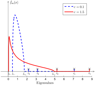
where $\mathcal{M}_{i}$ is the set indexes corresponding to the $j$-th eigenvalue of $\mathbf{R}$ (for example $\mathcal{M}_{r+1}=\left\{r+1,\cdots,m\right\}$ for $\lambda_{r+1}$). Two representations of $\hat{f}_{m}(x)$ for two different $c$ and a sufficient large $m$ are shown on Fig. 1 when the eigenvalues of $\mathbf{R}$ are 1, 2, 3, and 7 with the same multiplicity, where the eigenvalue 1 is the noise eigenvalue. One can observe that say (As6.S) is verified is equivalent to say that $\tau_{n-1}>\lambda_{+}$ and $\tau_{n+1}<\lambda_{-}$. In other words, all the sample eigenvalues corresponding to the non-unit eigenvalues of $\mathbf{R}$, converge to a value $\tau_{i}$ which is outside the support of the Marc̆enko-Pastur law (“asymptotic” PDF of the “unit” sample eigenvalues). As an illustration, one can notice that, in Fig. 1, for $\hat{f}_{m}(x)$ plotted for $c=0.1$, the separation condition is verified ($\omega_{1}=6$, $\omega_{2}=2$ and $\omega_{3}=1$ are greater that $\sqrt{c}=0.316$) and the three non-unit eigenvalues are represented on the PDF and outside the support of the Marc̆enko-Pastur law by their respective limits $\tau_{1}=7.116$, $\tau_{2}=3.15$ and $\tau_{3}=2.2$. On the contrary, for $\hat{f}_{m}(x)$ plotted for $c=1.5$, only the two greatest eigenvalues are represented on the PDF by their respective limits $\tau_{1}=8.75$ and $\tau_{2}=5.25$ while the separation condition is not verified for the eigenvalue $\lambda_{3}=2$ ($\omega_{3}=1<\sqrt{c}=1.223$). In this case, the sample eigenvalues corresponding to the eigenvalue $\lambda_{3}=2$ belongs to the Marc̆enko-Pastur law.

Figure 1: PDF of the eigenvalues of the SCM with the spiked model when the eigenvalues of $\mathbf{R}$ are 1, 2, 3, and 7 with the same multiplicity, where 1 is the noise eigenvalue.

III-C Convergence of simple quadratic forms

Here, we compare the convergence of two QFs in two convergence regimes: when $K\rightarrow\infty$ with a fixed $m$ and when $m,K\rightarrow\infty$ at the same rate.
We first present the useful convergences of simple QFs function of $\mathbf{\hat{R}}$. It is well known that, due to the strong law of large numbers, when $K\rightarrow\infty$ with a fixed $m$, $\mathbf{\hat{R}}\rightarrow\mathbf{R}$ a.s. [38]. Thus,

$$\bm{s}_{1}^{H}\mathbf{\hat{R}}^{-1}\bm{s}_{2}\underset{\underset{m<\infty}{\small{K\rightarrow\infty}}}{\overset{\text{a.s.}}{\longrightarrow}}\bm{s}_{1}^{H}\mathbf{R}^{-1}\bm{s}_{2}$$ (27)

Moreover, when $m,K\rightarrow\infty$ at the same rate [39, 19]:

$$\bm{s}_{1}^{H}\mathbf{\hat{R}}^{-1}\bm{s}_{2}\underset{\underset{m/K\to c<\infty}{\small{m,K\rightarrow\infty}}}{\overset{\text{a.s.}}{\longrightarrow}}\left(1-c\right)^{-1}\bm{s}_{1}^{H}\mathbf{R}^{-1}\bm{s}_{2}$$ (28)

The useful convergences of simple QFs function of $\hat{\bm{\Pi}}_{\mathrm{c}}^{\bot}$ are then presented. As $\mathbf{\hat{R}}\rightarrow\mathbf{R}$ a.s. when $K\rightarrow\infty$ with a fixed $m$, $\hat{\bm{\Pi}}_{\mathrm{c}}^{\bot}\rightarrow\bm{\Pi}_{\mathrm{c}}^{\bot}$ a.s. [19] in the same convergence regime. Thus:

$$\bm{s}_{1}^{H}\hat{\bm{\Pi}}_{\mathrm{c}}^{\bot}\bm{s}_{2}\>\underset{\underset{m<\infty}{\small{K\rightarrow\infty}}}{\overset{\text{a.s.}}{\longrightarrow}}\,\bm{s}_{1}^{H}\bm{\Pi}_{\mathrm{c}}^{\bot}\bm{s}_{2}$$ (29)

For the convergences in the large dimensional regime ($m,K\rightarrow\infty$ at the same rate), the convergences are presented under (As1-As5) and the separation condition As6.S. [22] showed that, $\forall i\in[\![1,\bar{M}-1]\!]$:

$$\bm{s}_{1}^{H}\mathbf{\hat{U}}_{i}\mathbf{\hat{U}}_{i}^{H}\bm{s}_{2}\underset{\underset{m/K\to c<\infty}{\small{m,K\rightarrow\infty}}}{\overset{\text{a.s.}}{\longrightarrow}}\dfrac{1-c\omega_{i}^{-2}}{1+c\omega_{i}^{-1}}\bm{s}_{1}^{H}\mathbf{U}_{i}\mathbf{U}_{i}^{H}\bm{s}_{2}$$ (30)

with $\omega_{i}=\lambda_{i}-1$. $\lambda_{i}$ is the $i$-th distinct eigenvalue of $\mathbf{R}$. Let $\chi_{i}=\dfrac{1-c\omega_{i}^{-2}}{1+c\omega_{i}^{-1}}$. Thus, using the following relationship,

$$\hat{\bm{\Pi}}_{\mathrm{c}}^{\bot}=\mathbf{I}_{m}-\sum_{i=1}^{\bar{M}-1}\mathbf{\hat{U}}_{i}\mathbf{\hat{U}}_{i}^{H}=\mathbf{I}_{m}-\sum_{i=1}^{r}\bm{\hat{u}}_{i}\bm{\hat{u}}_{i}^{H}$$ (31)

one can deduce that with the spiked model and in the large dimensional regime:

$$\bm{s}_{1}^{H}\hat{\bm{\Pi}}_{\mathrm{c}}^{\bot}\bm{s}_{2}\underset{\underset{m/K\to c<\infty}{\small{m,K\rightarrow\infty}}}{\overset{\text{a.s.}}{\longrightarrow}}\bm{s}_{1}^{H}\bar{\bm{\Pi}}_{\mathrm{c,S}}^{\bot}\bm{s}_{2}$$ (32)

with $\bar{\bm{\Pi}}_{\mathrm{c,S}}^{\bot}=\sum_{i=1}^{m}\psi_{i}\bm{u}_{i}\bm{u}_{i}^{H}$ and

$$\psi_{i}=\begin{cases}1,\;\,\qquad\quad\mathrm{if}\;i>r\\ 1-\chi_{i},\;\quad\mathrm{if}\;i\leqslant r\end{cases}$$ (33)

Consequently, $\bm{s}_{1}^{H}\hat{\mathbf{R}}^{-1}\bm{s}_{2}$ is consistent in the two convergence regimes and, although $\bm{s}_{1}^{H}\hat{\bm{\Pi}}_{\mathrm{c}}^{\bot}\bm{s}_{2}$ is consistent when $K\rightarrow\infty$ with a fixed $m$, it is no more consistent under the regime of interest i.e. when both $m,K\rightarrow\infty$ at the same rate.

IV New convergence results

IV-A Convergence of structured quadratic forms

In this section, the convergence of the structured QF function of $\hat{\bm{\Pi}}_{\mathrm{c}}^{\bot}$ is analyzed and results to Proposition 1.
Proposition 1: Let $\mathbf{B}$ be a $m\times m$ deterministic complex matrix with a uniformly bounded spectral norm for all $m$. Then, under (As1-As5, As6.S) and the spiked model,

$$\begin{array}[]{l}\bm{s}_{1}^{H}\hat{\bm{\Pi}}_{\mathrm{c}}^{\bot}\mathbf{B}\hat{\bm{\Pi}}_{\mathrm{c}}^{\bot}\bm{s}_{2}\underset{\underset{m/K\to c<\infty}{\small{m,K\rightarrow\infty}}}{\overset{\text{a.s.}}{\longrightarrow}}\bm{s}_{1}^{H}\bar{\bm{\Pi}}_{\mathrm{c,S}}^{\bot}\mathbf{B}\bar{\bm{\Pi}}_{\mathrm{c,S}}^{\bot}\bm{s}_{2}\end{array}$$ (35)

where $\bar{\bm{\Pi}}_{\mathrm{c,S}}^{\bot}=\sum_{i=1}^{m}\psi_{i}\bm{u}_{i}\bm{u}_{i}^{H}$ with $\psi_{i}$ defined by Eq.(33).

$\blacksquare$

Proof: See Appendix.

Moreover, one can remark that if $\mathbf{B}=\mathbf{R}$, where $\mathbf{R}$ is the covariance matrix as defined in Eq.(5), the following convergence holds:

$$\begin{array}[]{l}\bm{s}_{1}^{H}\hat{\bm{\Pi}}_{\mathrm{c}}^{\bot}\mathbf{R}\hat{\bm{\Pi}}_{\mathrm{c}}^{\bot}\bm{s}_{2}\underset{\underset{m/K\to c<\infty}{\small{m,K\rightarrow\infty}}}{\overset{\text{a.s.}}{\longrightarrow}}\bm{s}_{1}^{H}\bar{\bm{\Pi}}_{\mathrm{c,S}}^{\bot}\mathbf{R}\bar{\bm{\Pi}}_{\mathrm{c,S}}^{\bot}\bm{s}_{2}\end{array}$$ (37)

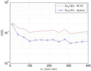
A visualization of the convergence of Eq.(35) in terms of Mean Squared Error (MSE) can be found in Fig. 2 when $m,K\rightarrow\infty$ at a fixed ratio. It is compared to the MSE corresponding to the following convergence when $K\rightarrow\infty$ with a fixed $m$:

$$\begin{array}[]{l}\bm{s}_{1}^{H}\hat{\bm{\Pi}}_{\mathrm{c}}^{\bot}\mathbf{B}\hat{\bm{\Pi}}_{\mathrm{c}}^{\bot}\bm{s}_{2}\underset{\underset{m<\infty}{\small{K\rightarrow\infty}}}{\overset{\text{a.s.}}{\longrightarrow}}\bm{s}_{1}^{H}\bm{\Pi}_{\mathrm{c}}^{\bot}\mathbf{B}\bm{\Pi}_{\mathrm{c}}^{\bot}\bm{s}_{2}\end{array}$$ (39)

Figure 2: MSE over $10^{3}$ iterations corresponding to Eq.(35) and Eq.(39) when the eigenvalues of $\mathbf{R}$ are 1, 21, 31, and 71 with the multiplicity $m-3$, 1, 1 and 1 respectively, $c=0.1$, $\bm{s}_{1}=\bm{s}_{2}$ are steering vectors of the LR noise component $\bm{c}$ and $\mathbf{B}=\mathbf{R}$.

IV-B Convergence of SINR losses

Now, we provide the convergences of the estimated SINR loss using the convergences previously presented and the following convergence. We recall that, as $\hat{\mathbf{R}}\rightarrow\mathbf{R}$ a.s. when $K\rightarrow\infty$ with a fixed $m$, one has:

$$\bm{s}_{1}^{H}\mathbf{\hat{R}}^{-1}\mathbf{R}\mathbf{\hat{R}}^{-1}\bm{s}_{2}\underset{\underset{m<\infty}{\small{K\rightarrow\infty}}}{\overset{\text{a.s.}}{\longrightarrow}}\bm{s}_{1}^{H}\mathbf{R}^{-1}\bm{s}_{2}$$ (40)

Hence, when $K\rightarrow\infty$ with a fixed $m$ and using Eq.(27), Eq.(40) and the continuous mapping theorem [38]:

$$\hat{\rho}\underset{\underset{m<\infty}{\small{K\rightarrow\infty}}}{\overset{\text{a.s.}}{\longrightarrow}}\frac{|\bm{a}^{H}\mathbf{R}^{-1}\bm{a}|^{2}}{(\bm{a}^{H}\mathbf{R}^{-1}\bm{a})(\bm{a}^{H}\mathbf{R}^{-1}\bm{a})}=1$$ (41)

And, under (As1-As5), when $m,K\rightarrow\infty$ at the same rate, from [33], we have:

$$\small\hat{\rho}\underset{\underset{m/K\to c<\infty}{\small{m,K\rightarrow\infty}}}{\overset{\text{a.s.}}{\longrightarrow}}\!\!\frac{(1-c)|\bm{a}^{H}\mathbf{R}^{-1}\bm{a}|^{2}}{(\bm{a}^{H}\mathbf{R}^{-1}\bm{a})(\bm{a}^{H}\mathbf{R}^{-1}\bm{a})}=1-c$$ (42)

Thus, the estimated SINR loss $\hat{\rho}$ is consistent when $K\rightarrow\infty$ with $m$ fixed and when $m,K\rightarrow\infty$ at the same rate, up to an additive constant $c$. Consequently, RMT cannot help us to improve the estimation of the theoretical SINR loss.
For the SINR loss corresponding to the adaptive LR filters, when $K\rightarrow\infty$ with a fixed $m$, using Eq.(29), Eq.(39) and the continuous mapping theorem theorem, we have:

$$\hat{\rho}_{\mathrm{LR}}\underset{\underset{m<\infty}{\small{K\rightarrow\infty}}}{\overset{\text{a.s.}}{\longrightarrow}}\rho_{\mathrm{LR}}$$ (43)

where $\rho_{\mathrm{LR}}$ is defined by Eq.(14). When $m,K\rightarrow\infty$ at the same rate, we obtain the following convergence:

$$\hat{\rho}_{\mathrm{LR}}\underset{\underset{m/K\to c<\infty}{\small{m,K\rightarrow\infty}}}{\overset{\text{a.s.}}{\longrightarrow}}\bar{\rho}_{\mathrm{LR}}^{(\mathrm{S})}=\rho_{\mathrm{LR}}|_{\bm{\Pi}_{\mathrm{c}}^{\bot}=\bm{\bar{\Pi}}_{\mathrm{c},\mathrm{S}}^{\bot}}\neq\rho_{\mathrm{LR}}$$ (44)

where Eq.(32), Proposition 1 and the continuous mapping theorem were used to prove Eq.(44). One can observe that, although the traditional estimator of $\rho_{\mathrm{LR}}$ is consistent when $K\rightarrow\infty$ with a fixed $m$, it is no more consistent when $m,K\rightarrow\infty$ at the same rate. It is also important to underline that the new convergence result leads to a more precise approximation of $\hat{\rho}_{\mathrm{LR}}$ than previous works [16]. Indeed, [16] proposes an approximation dependent on $K$ and the approximation proposed here depends on $K$ (and of course on $c$) as well as on the parameter $\bm{\Theta}$.

V Simulations

V-A Parameters

As an illustration of the interest of the application of RMT in filtering, the jamming application is chosen. The purpose of this application is to detect a target thanks to a ULA composed of $m$ sensors despite the presence of jamming. The response of the jamming, $\bm{c}$ is composed of signals similar to the target response. In this section, except for the convergences when $m,K\rightarrow\infty$ at the same rate $c$, we choose $m=100$ in order to have a large number for the data dimension. Even if, in some basic array processing applications, this number could seem significant, it actually became standard in many applications such as STAP [2], MIMO applications [40, 41], MIMO-STAP [40], etc. Here, $\bm{\Theta}=\theta$ where $\theta$ is the AoA. The jamming is composed of three synthetic targets with AoA $-20^{\circ}$, $0^{\circ}$ and $20^{\circ}$ and wavelength $l_{0}=0.667$m. Thus, the jamming (LR noise) has a rank $r=3$. Then, the AWGN $\bm{b}$ power is $\sigma^{2}=1$. Finally, the theoretical covariance matrix of the total noise can be written as $\mathbf{R}=\frac{JNR}{\mathrm{tr}(\bm{\Lambda})}\mathbf{U}\bm{\Lambda}\mathbf{U}^{H}+\sigma^{2}\mathbf{I}_{m}$ with $\bm{\Lambda}=\mathrm{diag([6,2,1])}$ and where $JNR$ is the jamming to noise ratio. $\frac{JNR}{\mathrm{tr}(\bm{\Lambda})}$ is fixed at $10$dB except for Fig. 4.
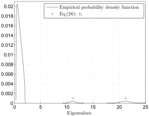
In order to validate the spiked model as covariance matrix model, we visualize a zoom of the experimental PDF of the eigenvalues of our data without target in Fig. 3 over $5\times 10^{4}$ Monte-Carlo iterations. We observe a Marc̆enko-Pastur law around 1 (eigenvalues of the white noise) and Gaussian distributions for the eigenvalues of the jamming, which is consistent to the CLT for the spiked model proved in [22]. The spiked model is consequently relevant for our data model.

Figure 3: Zoom of the experimental PDF of jamming plus noise data with $c=0.2$ and $\frac{JNR}{\mathrm{tr}(\bm{\Lambda})}=10$dB.

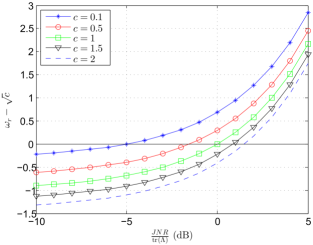
Moreover, in order to verified that the spiked model is realistic in terms of separation condition, Fig. 4 shows ($\omega_{r}-\sqrt{c}$) as a function of $\frac{JNR}{\mathrm{tr}(\bm{\Lambda})}$ in dB. This figure will be the same for all $m$ and $K$ at a fixed ratio. We recall that, in order to satisfy the separation condition, one should have $\omega_{r}-\sqrt{c}>0$. Consequently, we gladly observe that it is satisfied for $\frac{JNR}{\mathrm{tr}(\bm{\Lambda})}>4$dB for the majority of $c$ even $c>2$. Indeed, in practice, if the $\frac{JNR}{\mathrm{tr}(\bm{\Lambda})}$ is lower, the jamming will not have any effects on the performance.

Figure 4: Separation condition ($\omega_{r}-\sqrt{c}$) of the spiked model for the lowest non-unit eigenvalue as a function of the ratio $\frac{JNR}{\mathrm{tr}(\bm{\Lambda})}$ in dB.

V-B Performance of filters

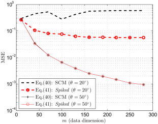
We now observe the performances of filters through the SINR loss. We are first interested in the validation of the convergence of $\hat{\rho}_{\mathrm{LR}}$ in Eq.(44) as $m,K\rightarrow\infty$ at the same rate. This convergence is validated and presented in Fig. 5 in terms of MSE over $10^{3}$ realizations with $c=3$ for an AoA of the target ($\theta=50^{\circ}$) and an AoA of the jamming ($\theta=20^{\circ}$).

Figure 5: MSE corresponding to Eq.(43) and Eq.(44) when $m,K\rightarrow\infty$ at a fixed ratio $c=3$ and $\frac{JNR}{\mathrm{tr}(\bm{\Lambda})}=10$dB.

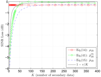
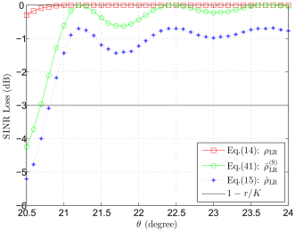
Fig. 6 shows the visualization of Eq.(14) (blue line with stars), Eq.(15) (blue dashed line), the right side of the convergence in Eq.(44) (green line with circles) and the approximation $\mathbb{E}[\hat{\rho}_{\mathrm{LR}}]\simeq 1-\frac{r}{K}$ introduced by [16] (black line) as a function of $K$ when the target is near from the jamming, i.e. $\theta=20.5^{\circ}$. We observe that the spiked model and the RMT helps us to obtain a better estimation of $\mathbb{E}[\hat{\rho}_{\mathrm{LR}}]$ than the estimation $\mathbb{E}[\hat{\rho}_{\mathrm{LR}}]\simeq 1-\frac{r}{K}$ as the curve of $\bar{\rho}_{\mathrm{LR}}^{(\mathrm{S})}$ has the same behavior as the curve of $\hat{\rho}_{\mathrm{LR}}$. Then, similarly, the same equations are visualized as a function of $\theta$ in Fig. 7 with $K=2r$. We observe that, unlike the estimation $1-r/K$, the RMT with the spiked model permits us to obtain a better estimation of $\mathbb{E}[\hat{\rho}_{\mathrm{LR}}]$ as a function of $\theta$ and consequently a better approximation of its behavior. Thus, it permits to predict the parameter $\theta$ value corresponding to the performance break (here around $21.1^{\circ}$).

Figure 6: Visualization of Eq.(14) (red line with squares), Eq.(15) (blue dashed line), the right side of the convergence in Eq.(44) (green line with circles) and the traditional estimation of $\mathbb{E}[\hat{\rho}_{\mathrm{LR}}]$ (black line) as a function of $K$ (over $10^{3}$ realizations) with $\frac{JNR}{\mathrm{tr}(\bm{\Lambda})}=10$dB, $m=100$ and $\theta=20.5^{\circ}$.

Figure 7: Visualization of Eq.(14) (red line with squares), Eq.(15) (blue dashed line), the right side of the convergence in Eq.(44) (green line with circles) and the traditional estimation of $\mathbb{E}[\hat{\rho}_{\mathrm{LR}}]$ (black line) as a function of $\theta$ (over $10^{3}$ realizations) with $\frac{JNR}{\mathrm{tr}(\bm{\Lambda})}=10$dB, $m=100$ and $K=2r$.

VI Conclusion

In this paper, we proposed new results in random matrix theory with a specific covariance matrix model fitted to our data model: the spiked model. Based on this, we studied the convergence of the traditional estimators of the SINR loss in their full rank and low rank version when the number of secondary data $K\rightarrow\infty$ with a fixed data dimension $m$ and when $m,K\rightarrow\infty$ at the same rate $c=m/K$. We observed that the full rank version is consistent in the two regimes. However, the low rank version is consistent when $K\rightarrow\infty$ with a fixed $m$ but is not consistent when $m,K\rightarrow\infty$ at the same rate $c$. Finally, we applied these results to a jamming application. We first observed that the experimental probability density function of the eigenvalue of the covariance matrix of jamming data is relevant with the probability density function of the spiked model. Then, we validated the convergence of the SINR loss in its low rank version and we observed that random matrix theory and more precisely the spiked model better evaluate the asymptotic performances of the low rank SINR loss corresponding to the adaptive LR filter, especially when the steering vector parameter is close to the jamming one and contrary to previous works. Moreover, it permits to predict the steering vector parameter value corresponding to the performance break.

VII Appendix

The proof is decomposed as follows. We first develop the structured QF as a sum of simple QFs and base structured QF (Subsec. VII-A). In a second time, we formulate the base structured QF as a complex integral (Subsec. VII-B) and split it into several integrals (Subsec. VII-C). Then, we determine the deterministic complex integral equivalent of the base structured QF (Subsec. VII-D) and its formal expression (Subsec. VII-E). Finally, we use this result to determine the convergence of the structured QF in the large dimensional regime (Subsec. VII-F). The regime of convergences in the Appendix, if not precised, is $m,K\rightarrow\infty$ at a fixed ratio $c$.

VII-A Development of the structured QF

Let $\bm{s}_{1}$ and $\bm{s}_{2}$ be two deterministic complex vectors and $\mathbf{B}$ be a $m\times m$ deterministic complex matrix with uniformly bounded spectral norm for all $m$. In order to obtain the convergence of the structured QF $\bm{s}_{1}^{H}\hat{\bm{\Pi}}_{\mathrm{c}}^{\bot}\mathbf{B}\hat{\bm{\Pi}}_{\mathrm{c}}^{\bot}\bm{s}_{2}$, one can rewrite, using the notations of Eq.(23) and the spiked model, $\hat{\bm{\Pi}}_{\mathrm{c}}^{\bot}=\hat{\bm{\Pi}}_{r+1}=\hat{\mathbf{U}}_{r+1}\hat{\mathbf{U}}_{r+1}^{H}=\mathbf{I}_{m}-\sum_{i=1}^{r}\hat{\bm{\Pi}}_{i}$ where $\hat{\mathbf{U}}_{r+1}=[\hat{\bm{u}}_{r+1},\cdots,\hat{\bm{u}}_{m}]$, $\hat{\bm{\Pi}}_{i}=\hat{\bm{u}}_{i}\hat{\bm{u}}_{i}^{H}$, $\forall i\in[\![1,r]\!]$ and $\hat{\bm{u}}_{i}$ are the eigenvectors of the SCM. We recall that $r$ is fixed for all $m$, i.e. $r/m\rightarrow 0^{+}$. Thus, one can develop the structured QF as :

$$\!\!\!\!\!\!\bm{s}_{1}^{H}\hat{\bm{\Pi}}_{\mathrm{c}}^{\bot}\mathbf{B}\hat{\bm{\Pi}}_{\mathrm{c}}^{\bot}\bm{s}_{2}\!\!\!\!\!\! = \!\!\!\!\!\!\bm{s}_{1}^{H}\left(\mathbf{I}_{m}-\sum_{i=1}^{r}\hat{\bm{\Pi}}_{i}\right)\mathbf{B}\left(\mathbf{I}_{m}-\sum_{i=1}^{r}\hat{\bm{\Pi}}_{i}\right)\bm{s}_{2}$$ (47)

$$= \!\!\!\!\!\!\bm{s}_{1}^{H}\mathbf{B}\bm{s}_{2}\!-\!\bm{s}_{1}^{H}\sum_{i=1}^{r}\hat{\bm{\Pi}}_{i}\mathbf{B}\bm{s}_{2}\!-\!\bm{s}_{1}^{H}\mathbf{B}\sum_{i=1}^{r}\hat{\bm{\Pi}}_{i}\bm{s}_{2}$$

$$+\bm{s}_{1}^{H}\sum_{i=1}^{r}\hat{\bm{\Pi}}_{i}\mathbf{B}\sum_{i=1}^{r}\hat{\bm{\Pi}}_{i}\bm{s}_{2}$$

$$= \!\!\!\!\!\!\bm{s}_{1}^{H}\mathbf{B}\bm{s}_{2}\!-\!\sum_{i=1}^{r}\left(\bm{s}_{1}^{H}\hat{\bm{\Pi}}_{i}\mathbf{B}\bm{s}_{2}+\bm{s}_{1}^{H}\mathbf{B}\hat{\bm{\Pi}}_{i}\bm{s}_{2}\right)$$

$$\!\!\!\!\!\!+\!\!\sum_{j_{1}=1}^{r}\!\bm{s}_{1}^{H}\hat{\bm{\Pi}}_{j_{1}}\mathbf{B}\hat{\bm{\Pi}}_{j_{1}}\bm{s}_{2}\!+\!\!\!\!\sum_{\underset{j_{1}\neq j_{2}}{j_{1},j_{2}=1}}^{r}\!\!\!\!\bm{s}_{1}^{H}\hat{\bm{\Pi}}_{j_{1}}\mathbf{B}\hat{\bm{\Pi}}_{j_{2}}\bm{s}_{2}$$

VII-B Formulation of the base structured QF as a complex integral

Remarking that Eq.(47) is a sum of simple QFs and base structured QFs, we first focus on the convergence of the base structured QF $\hat{\eta}(j_{1},j_{2})=\bm{s}_{1}^{H}\hat{\bm{\Pi}}_{j_{1}}\mathbf{B}\hat{\bm{\Pi}}_{j_{2}}\bm{s}_{2}$, $\left\{j_{1},j_{2}\right\}\in[\![1,r]\!]^{2}$. Let us now formulate the base structured QF as a complex integral.
Proposition 2: Let $\mathbf{B}$ be a $m\times m$ deterministic complex matrix with a uniformly bounded spectral norm for all $m$. Then, under (As1-As5, As6.S) and the spiked model, $\forall j_{1},j_{2}\in[\![1,r+1]\!]$, if $\hat{\eta}(j_{1},j_{2})=\bm{s}_{1}^{H}\hat{\bm{\Pi}}_{j_{1}}\mathbf{B}\hat{\bm{\Pi}}_{j_{2}}\bm{s}_{2}$:

$$\hat{\eta}(j_{1},j_{2}) = \dfrac{1}{(2i\pi)^{2}}\oint_{\mathcal{C}_{j_{1}}^{-}}\oint_{\mathcal{C}_{j_{2}}^{-}}\bm{s}_{1}^{H}\left(\hat{\mathbf{R}}-z_{1}\mathbf{I}_{m}\right)^{-1}$$ (48)

$$\times\mathbf{B}\left(\hat{\mathbf{R}}-z_{2}\mathbf{I}_{m}\right)^{-1}\bm{s}_{2}dz_{1}dz_{2}$$

$\blacksquare$

Proof: If $j_{1}\neq j_{2}$, it can be easily shown that $\hat{\eta}(j_{1},j_{2})$ can be expressed as the following Cauchy integral:

$$A\!=\!\frac{1}{(2i\pi)^{2}}\!\oint_{\mathcal{C}_{j_{1}}^{-}}\!\!\oint_{\mathcal{C}_{j_{2}}^{-}}\!\!\!\bm{s}_{1}^{H}\!(\hat{\mathbf{R}}-z_{1}\mathbf{I}_{m})^{-1}\mathbf{B}(\hat{\mathbf{R}}-z_{2}\mathbf{I}_{m})^{-1}\bm{s}_{2}dz_{1}dz_{2}$$ (49)

where $\mathcal{C}_{j}^{-}$ in a negatively oriented contour encompassing the eigenvalues of $\hat{\mathbf{R}}$ corresponding to the $j$-th eigenvalue of $\mathbf{R}$ and $z_{1}$ and $z_{2}$ are independent variables. Indeed, let $\mathbf{G}(z_{k})=(\hat{\mathbf{R}}-z_{k}\mathbf{I}_{m})^{-1}=(\frac{1}{K}\mathbf{X}\mathbf{X}^{H}-z_{k}\mathbf{I}_{m})^{-1}$ with $k\in\left\{1,2\right\}$. Thus:

$$\!\!\!\!\!\!A\!\!\!\!\! = \!\!\!\!\!\dfrac{1}{(2i\pi)^{2}}\!\oint_{\mathcal{C}_{j_{1}}^{-}}\!\!\oint_{\mathcal{C}_{j_{2}}^{-}}\!\!\!\bm{s}_{1}^{H}\mathbf{G}(z_{1})\mathbf{B}(\hat{\mathbf{R}}-z_{2}\mathbf{I}_{m})^{-1}\!\bm{s}_{2}dz_{1}dz_{2}$$ (51)

$$= \!\!\!\!\!\frac{1}{(2i\pi)^{2}}\!\oint_{\mathcal{C}_{j_{1}}^{-}}\!\!\!\oint_{\mathcal{C}_{j_{2}}^{-}}\!\!\!\!\bm{s}_{1}^{H}\mathbf{G}(z_{1})\mathbf{B}\!\left(\sum_{n=1}^{m}\!\hat{\lambda}_{n}\hat{\bm{u}}_{n}\hat{\bm{u}}_{n}^{H}\!-\!z_{2}\mathbf{I}_{m}\!\right)^{-1}$$

$$\qquad\qquad\qquad\qquad\qquad\qquad\qquad\qquad\times\bm{s}_{2}dz_{2}dz_{1}$$

$$= \!\!\!\!\!\frac{1}{(2i\pi)^{2}}\oint_{\mathcal{C}_{j_{1}}^{-}}\oint_{\mathcal{C}_{j_{2}}^{-}}\sum_{n=1}^{m}\frac{\bm{s}_{1}^{H}\mathbf{G}(z_{1})\mathbf{B}\hat{\bm{u}}_{n}\hat{\bm{u}}_{n}^{H}\bm{s}_{2}}{\hat{\lambda}_{n}-z_{2}}dz_{2}dz_{1}$$ (52)

$$= \!\!\!\!\!\frac{1}{2i\pi}\oint_{\mathcal{C}_{j_{1}}^{-}}\sum_{n=1}^{m}\frac{1}{2i\pi}\oint_{\mathcal{C}_{j_{2}}^{-}}f_{n}^{(2)}(z_{2})dz_{2}dz_{1}$$ (53)

where $f_{n}^{(2)}(z_{2})=\frac{\bm{s}_{1}^{H}\mathbf{G}(z_{1})\mathbf{B}\hat{\bm{u}}_{n}\hat{\bm{u}}_{n}^{H}\bm{s}_{2}}{\hat{\lambda}_{n}-z_{2}}$. From the expression $f_{n}^{(2)}(z_{2})$, one observe that $f_{n}^{(2)}(z_{2})$ has a single simple pole $\hat{\lambda}_{n}$ which is encompassed by $\mathcal{C}_{j_{2}}^{-}$ for the indexes $n\in\mathcal{M}_{j_{2}}$ where $\mathcal{M}_{j_{2}}$ is the set of indexes corresponding to the $j_{2}$-th eigenvalue of $\mathbf{R}$. Consequently, from complex analysis:

$$A = \frac{1}{2i\pi}\oint_{\mathcal{C}_{j_{1}}^{-}}\sum_{n\in\mathcal{M}_{j_{2}}}\frac{1}{2i\pi}\oint_{\mathcal{C}_{j_{2}}^{-}}\frac{\bm{s}_{1}^{H}\mathbf{G}(z_{1})\mathbf{B}\hat{\bm{u}}_{n}\hat{\bm{u}}_{n}^{H}\bm{s}_{2}}{\hat{\lambda}_{n}-z_{2}}dz_{2}dz_{1}$$ (55)

$$= \frac{1}{2i\pi}\oint_{\mathcal{C}_{j_{1}}^{-}}\sum_{n\in\mathcal{M}_{j_{2}}}\frac{1}{2i\pi}\oint_{\mathcal{C}_{j_{2}}^{-}}f^{(2)}_{n}(z_{2})dz_{2}dz_{1}$$

$$= \frac{1}{2i\pi}\oint_{\mathcal{C}_{j_{1}}^{-}}\sum_{n\in\mathcal{M}_{j_{2}}}\left[-\mathrm{Res}\left(f^{(2)}_{n}(z_{2}),\hat{\lambda}_{n}\right)\right]dz_{1}$$ (56)

where $\mathrm{Res}\left(f^{(2)}_{n}(z_{2}),\hat{\lambda}_{n}\right)$ is the residue of $f^{(2)}_{n}(z_{2})$ at $\hat{\lambda}_{n}$. Thus, using the residue theorem and residue calculus:

$$\!\!\!\!\!\!\!\!A\!\!\!\!\! = \!\!\!\!\!\frac{1}{2i\pi}\oint_{\mathcal{C}_{j_{1}}^{-}}\sum_{n\in\mathcal{M}_{j_{2}}}\left[-\underset{z_{2}\rightarrow\hat{\lambda}_{n}}{\mathrm{lim}}(z_{2}-\hat{\lambda}_{n})f^{(2)}_{n}(z_{2})\right]dz_{1}$$

$$= \!\!\!\!\!\frac{1}{2i\pi}\!\oint_{\mathcal{C}_{j_{1}}^{-}}\!\sum_{n\in\mathcal{M}_{j_{2}}}\!\!\!\underset{z_{2}\rightarrow\hat{\lambda}_{n}}{\mathrm{lim}}\!\!\!\left\{(\hat{\lambda}_{n}-z_{2})\frac{\bm{s}_{1}^{H}\mathbf{G}(z_{1})\mathbf{B}\hat{\bm{u}}_{n}\hat{\bm{u}}_{n}^{H}\bm{s}_{2}}{\hat{\lambda}_{n}-z_{2}}\right\}dz_{1}$$

$$= \!\!\!\!\!\frac{1}{2i\pi}\oint_{\mathcal{C}_{j_{1}}^{-}}\sum_{n\in\mathcal{M}_{j_{2}}}\underset{z_{2}\rightarrow\hat{\lambda}_{n}}{\mathrm{lim}}\left\{\bm{s}_{1}^{H}\mathbf{G}(z_{1})\mathbf{B}\hat{\bm{u}}_{n}\hat{\bm{u}}_{n}^{H}\bm{s}_{2}\right\}dz_{1}$$ (59)

$$\!\!\!\!\!\!\!\!A\!\!\!\!\! = \!\!\!\!\!\frac{1}{2i\pi}\oint_{\mathcal{C}_{j_{1}}^{-}}\bm{s}_{1}^{H}\mathbf{G}(z_{1})\mathbf{B}\sum_{n\in\mathcal{M}_{j_{2}}}\hat{\bm{u}}_{n}\hat{\bm{u}}_{n}^{H}\bm{s}_{2}dz_{1}$$ (60)

$$= \!\!\!\!\!\frac{1}{2i\pi}\oint_{\mathcal{C}_{j_{1}}^{-}}\bm{s}_{1}^{H}\left(\hat{\mathbf{R}}-z_{1}\mathbf{I}_{m}\right)^{-1}\mathbf{B}\hat{\bm{\Pi}}_{j_{2}}\bm{s}_{2}dz_{1}$$ (61)

$$= \!\!\!\!\!\frac{1}{2i\pi}\oint_{\mathcal{C}_{j_{1}}^{-}}\bm{s}_{1}^{H}\left(\sum_{n=1}^{m}\hat{\lambda}_{n}\hat{\bm{u}}_{n}\hat{\bm{u}}_{n}^{H}-z_{1}\mathbf{I}_{m}\right)^{-1}\mathbf{B}\hat{\bm{\Pi}}_{j_{2}}\bm{s}_{2}dz_{1}$$ (62)

$$= \!\!\!\!\!\frac{1}{2i\pi}\oint_{\mathcal{C}_{j_{1}}^{-}}\sum_{n=1}^{m}\frac{\bm{s}_{1}^{H}\hat{\bm{u}}_{n}\hat{\bm{u}}_{n}^{H}\mathbf{B}\hat{\bm{\Pi}}_{j_{2}}\bm{s}_{2}}{\hat{\lambda}_{n}-z_{1}}dz_{1}$$ (63)

$$= \!\!\!\!\!\sum_{n=1}^{m}\frac{1}{2i\pi}\oint_{\mathcal{C}_{j_{1}}^{-}}f^{(1)}_{n}(z_{1})dz_{1}$$ (64)

where $f_{n}^{(1)}(z_{1})=\frac{\bm{s}_{1}^{H}\hat{\bm{u}}_{n}\hat{\bm{u}}_{n}^{H}\mathbf{B}\hat{\bm{\Pi}}_{j_{2}}\bm{s}_{2}}{\hat{\lambda}_{n}-z_{1}}$. Similarly, $f_{n}^{(1)}(z_{1})$ has a single simple pole $\hat{\lambda}_{n}$ which is encompassed by $\mathcal{C}_{j_{1}}^{-}$ for the indexes $n\in\mathcal{M}_{j_{1}}$. Thus:

$$A = \sum_{n\in\mathcal{M}_{j_{1}}}\frac{1}{2i\pi}\oint_{\mathcal{C}_{j_{1}}^{-}}f^{(1)}_{n}(z_{1})dz_{1}$$ (65)

$$= -\sum_{n\in\mathcal{M}_{j_{1}}}\mathrm{Res}\left(f^{(1)}_{n}(z_{1}),\hat{\lambda}_{n}\right)$$ (66)

$$= -\sum_{n\in\mathcal{M}_{j_{1}}}\underset{z_{1}\rightarrow\hat{\lambda}_{n}}{\mathrm{lim}}(z_{1}-\hat{\lambda}_{n})f^{(1)}_{n}(z_{1})$$ (67)

$$= \sum_{n\in\mathcal{M}_{j_{1}}}\underset{z_{1}\rightarrow\hat{\lambda}_{n}}{\mathrm{lim}}\left\{(\hat{\lambda}_{n}-z_{1})\frac{\bm{s}_{1}^{H}\hat{\bm{u}}_{n}\hat{\bm{u}}_{n}^{H}\mathbf{B}\hat{\bm{\Pi}}_{j_{2}}\bm{s}_{2}}{\hat{\lambda}_{n}-z_{1}}\right\}$$ (68)

$$= \sum_{n\in\mathcal{M}_{j_{1}}}\underset{z_{1}\rightarrow\hat{\lambda}_{n}}{\mathrm{lim}}\left\{\bm{s}_{1}^{H}\hat{\bm{u}}_{n}\hat{\bm{u}}_{n}^{H}\mathbf{B}\hat{\bm{\Pi}}_{j_{2}}\bm{s}_{2}\right\}$$ (69)

$$= \bm{s}_{1}^{H}\sum_{n\in\mathcal{M}_{j_{1}}}\hat{\bm{u}}_{n}\hat{\bm{u}}_{n}^{H}\mathbf{B}\hat{\bm{\Pi}}_{j_{2}}\bm{s}_{2}=\bm{s}_{1}^{H}\hat{\bm{\Pi}}_{j_{1}}\mathbf{B}\hat{\bm{\Pi}}_{j_{2}}\bm{s}_{2}$$ (70)

Consequently, $\hat{\eta}(j_{1},j_{2})=A$ for $j_{1}\neq j_{2}$.
Then, if $j_{1}=j_{2}=j$ and using the same arguments as previously, one has:

$$\bm{s}_{1}^{H}\hat{\bm{\Pi}}_{j}\mathbf{B}\hat{\bm{\Pi}}_{j}\bm{s}_{2}=\dfrac{1}{2i\pi}\oint_{\mathcal{C}_{j}^{-}}\bm{s}_{1}^{H}\sum_{n=1}^{m}\dfrac{\hat{\bm{u}}_{n}\hat{\bm{u}}_{n}^{H}\mathbf{B}\hat{\bm{u}}_{n}\hat{\bm{u}}_{n}^{H}}{\hat{\lambda}_{n}-z}\bm{s}_{2}dz$$ (71)

However, the remaining of the proof is based on the fact that the resolvent $\mathbf{G}(z)$ of the SCM can be found in the complex integral, which is not the case in the previous equation. Consequently, noticing that:

$$g(\hat{\bm{\Pi}}_{j})=\dfrac{1}{2i\pi}\oint_{\mathcal{C}_{j}^{-}}\sum_{n=1}^{m}\dfrac{g(\hat{\bm{\Pi}}_{n})}{\hat{\lambda}_{n}-z}dz$$ (72)

where $g(.)$ is a functional, Eq.(71) is equivalent to Eq.(48). As a consequence, $\forall j_{1},j_{2}\in[\![1,r+1]\!]$:

$$\hat{\eta}(j_{1},j_{2}) = \dfrac{1}{(2i\pi)^{2}}\oint_{\mathcal{C}_{j_{1}}^{-}}\oint_{\mathcal{C}_{j_{2}}^{-}}\bm{s}_{1}^{H}\left(\hat{\mathbf{R}}-z_{1}\mathbf{I}_{m}\right)^{-1}$$ (73)

$$\times\mathbf{B}\left(\hat{\mathbf{R}}-z_{2}\mathbf{I}_{m}\right)^{-1}\bm{s}_{2}dz_{1}dz_{2}$$

VII-C Development of the complex integral

Next, one want to split the previous line integral into several line integrals where some of them will tend to 0. Thus, from [22], with $k\in\left\{1,2\right\}$, one can write:

$$(\hat{\mathbf{R}}-z_{k}\mathbf{I}_{m})^{-1}\!\!\!\! = \!\!\!\!(\mathbf{I}_{m}+\mathbf{P})^{-1/2}\left[\mathbf{Q}(z_{k})-z_{k}\mathbf{Q}(z_{k})\mathbf{U}\right.$$ (74)

$$\!\!\!\!\left.\times\mathbf{\hat{H}}(z_{k})^{-1}\bm{\Omega}(\mathbf{I}_{r}+\bm{\Omega})^{-1}\mathbf{U}^{H}\mathbf{Q}(z_{k})\right]$$

$$\!\!\!\!\times(\mathbf{I}_{m}+\mathbf{P})^{-1/2}$$

with

$$\mathbf{Q}(z_{k}) = (\tfrac{1}{K}\mathbf{Y}\mathbf{Y}^{H}-z_{k}\mathbf{I}_{m})^{-1}$$ (75)

$$\mathbf{\hat{H}}(z_{k}) = \mathbf{I}_{m}+z_{k}\bm{\Omega}(\mathbf{I}_{m}+\bm{\Omega})^{-1}\mathbf{U}^{H}\mathbf{Q}(z_{k})\mathbf{U}$$ (76)

Then, replacing $(\hat{\mathbf{R}}-z_{k}\mathbf{I}_{m})^{-1}$ by Eq.(74) in Eq.(48) and developing the obtained result, one obtains:

$$\hat{\eta}(j_{1},j_{2})\!\!\!\! = \dfrac{1}{(2i\pi)^{2}}\oint_{\mathcal{C}_{j_{1}}^{-}}\oint_{\mathcal{C}_{j_{2}}^{-}}\bm{s}_{1}^{H}\mathbf{E}(z_{1})\mathbf{B}\mathbf{E}(z_{2})\bm{s}_{2}dz_{1}dz_{2}$$ (77)

$$- \!\!\!\!\dfrac{1}{(2i\pi)^{2}}\oint_{\mathcal{C}_{j_{1}}^{-}}\oint_{\mathcal{C}_{j_{2}}^{-}}\left[\mathbf{\hat{e}}_{1}^{H}(z_{1})\mathbf{\hat{H}}(z_{1})^{-1}\mathbf{\hat{C}}_{2}(z_{1})\mathbf{B}\right]$$

$$\qquad\qquad\qquad\qquad\qquad\quad\times\mathbf{E}(z_{2})\bm{s}_{2}dz_{1}dz_{2}$$

$$- \!\!\!\!\dfrac{1}{(2i\pi)^{2}}\oint_{\mathcal{C}_{j_{1}}^{-}}\oint_{\mathcal{C}_{j_{2}}^{-}}\bm{s}_{1}^{H}\mathbf{E}(z_{1})\left[\mathbf{B}\mathbf{\hat{C}}_{1}^{H}(z_{2})\mathbf{\hat{H}}(z_{2})^{-1}\right.$$

$$\qquad\qquad\qquad\qquad\qquad\quad\times\left.\mathbf{\hat{e}}_{2}(z_{2})\right]dz_{1}dz_{2}$$

$$+ \!\!\!\!\dfrac{1}{(2i\pi)^{2}}\oint_{\mathcal{C}_{j_{1}}^{-}}\oint_{\mathcal{C}_{j_{2}}^{-}}\mathbf{\hat{e}}_{1}^{H}(z_{1})\mathbf{\hat{H}}(z_{1})^{-1}\mathbf{\hat{C}}_{2}(z_{1})\mathbf{B}$$

$$\qquad\quad\times\mathbf{\hat{C}}_{1}^{H}(z_{2})\mathbf{\hat{H}}(z_{2})^{-1}\mathbf{\hat{e}}_{2}(z_{2})dz_{1}dz_{2}$$

$$= D_{1}-D_{2}-D_{3}+D_{4}$$ (78)

with

$$\!\!\!\!\mathbf{E}(z)\!\!\!\! = \!\!\!\!(\mathbf{I}_{m}+\mathbf{P})^{-1/2}\mathbf{Q}(z)(\mathbf{I}_{m}+\mathbf{P})^{-1/2}$$ (79)

$$\!\!\!\!\mathbf{\hat{e}}_{1}^{H}(z)\!\!\!\! = \!\!\!\!\bm{s}_{1}^{H}(\mathbf{I}_{m}+\mathbf{P})^{-1/2}z\mathbf{Q}(z)\mathbf{U}$$ (80)

$$\!\!\!\!\mathbf{\hat{C}}_{2}(z)\!\!\!\! = \!\!\!\!\bm{\Omega}(\mathbf{I}_{m}+\bm{\Omega})^{-1}\mathbf{U}^{H}\mathbf{Q}(z)(\mathbf{I}_{m}+\mathbf{P})^{-1/2}$$ (81)

$$\!\!\!\!\mathbf{\hat{C}}_{1}^{H}(z)\!\!\!\! = \!\!\!\!(\mathbf{I}_{m}+\mathbf{P})^{-1/2}z\mathbf{Q}(z)\mathbf{U}$$ (82)

$$\!\!\!\!\mathbf{\hat{e}}_{2}(z)\!\!\!\! = \!\!\!\!\bm{\Omega}(\mathbf{I}_{m}+\bm{\Omega})^{-1}\mathbf{U}^{H}\mathbf{Q}(z)(\mathbf{I}_{m}+\mathbf{P})^{-1/2}\bm{s}_{2}$$ (83)

VII-D Determination of the deterministic complex integral equivalent

The convergence of the terms $D_{1}$ to $D_{4}$ has now to be studied. Some of them will tend to 0 and the remainder of the terms will tend to a deterministic integral equivalent.
Proposition 3: Let $\mathbf{B}$ be a $m\times m$ deterministic complex matrix with a uniformly bounded spectral norm for all $m$. Then, under (As1-As5, As6.S) and the spiked model, $\forall j_{1},j_{2}\in[\![1,r+1]\!]$, $\hat{\eta}(j_{1},j_{2})-\eta(j_{1},j_{2})\overset{\mathrm{a.s.}}{\longrightarrow}0$ with

$$\eta(j_{1},j_{2})\!\!\!\! = \!\!\!\!\dfrac{1}{(2i\pi)^{2}}\oint_{\gamma_{j_{1}}^{-}}\oint_{\gamma_{j_{2}}^{-}}\mathbf{e}_{1}^{H}(z_{1})\mathbf{H}(z_{1})^{-1}\mathbf{C}_{2}(z_{1})$$ (84)

$$\quad\times\mathbf{B}\mathbf{C}_{1}^{H}(z_{2})\mathbf{H}(z_{2})^{-1}\mathbf{e}_{2}(z_{2})dz_{1}dz_{2}$$

where $\gamma_{j}^{-}$ is a deterministic negatively oriented circle only enclosing $\tau_{j}$ (cf. Eq.(26)) and

$$\mathbf{H}(z) = \mathbf{I}_{m}+z\bar{b}_{m}(z)\bm{\Omega}(\mathbf{I}_{m}+\bm{\Omega})^{-1}$$ (85)

$$\mathbf{e}_{1}^{H}(z) = z\bar{b}_{m}(z)\bm{s}_{1}^{H}(\mathbf{I}_{m}+\mathbf{P})^{-1/2}\mathbf{U}$$ (86)

$$\mathbf{C}_{2}(z) = \bar{b}_{m}(z)\bm{\Omega}(\mathbf{I}_{m}+\bm{\Omega})^{-1}\mathbf{U}^{H}(\mathbf{I}_{m}+\mathbf{P})^{-1/2}$$ (87)

$$\mathbf{C}_{1}^{H}(z) = z\bar{b}_{m}(z)(\mathbf{I}_{m}+\mathbf{P})^{-1/2}\mathbf{U}$$ (88)

$$\mathbf{e}_{2}(z) = \bar{b}_{m}(z)\bm{\Omega}(\mathbf{I}_{m}+\bm{\Omega})^{-1}\mathbf{U}^{H}(\mathbf{I}_{m}+\mathbf{P})^{-1/2}\bm{s}_{2}$$ (89)

$\blacksquare$

Proof: We first recall that we are interested in the indexes $j_{1},j_{2}\in[\![1,r]\!]$. Then, the function $\mathbf{E}(z)$ in $D_{1}$, $D_{2}$ and $D_{3}$ can be rewritten as:

$$\mathbf{E}(z)=\left(\hat{\mathbf{R}}-z(\mathbf{I}_{m}+\mathbf{P})\right)^{-1}=\sum_{n=1}^{m}\dfrac{\hat{\bm{u}}_{n}\hat{\bm{u}}_{n}^{H}}{\hat{\lambda}_{n}-z(1+\omega_{n})}$$ (90)

Thus, $\mathbf{E}(z_{1})$ (resp. $\mathbf{E}(z_{2})$) has a single simple pole $\frac{\hat{\lambda}_{n}}{1+\omega_{n}}\neq\hat{\lambda}_{n}$ when $\omega_{n}\neq 0$, i.e. $n\in[\![1,r]\!]$ ((As5, As6.S) are verified and $\hat{f}(x)\rightarrow f(x)$, with probability one for all large $m,K$ at a fixed ratio $c$). As a consequence, $\forall j_{1},j_{2}\in[\![1,r]\!]$, $\mathcal{C}_{j_{1}}^{-}$ (resp. $\mathcal{C}_{j_{2}}^{-}$) does not encompass $\mathbf{E}(z_{1})$ (resp. $\mathbf{E}(z_{2})$). Thus, $D_{1}=D_{2}=D_{3}=0$ and:

$$\hat{\eta}(j_{1},j_{2})\!\!\!\! = \!\!\!\!\dfrac{1}{(2i\pi)^{2}}\oint_{\mathcal{C}_{j_{1}}^{-}}\oint_{\mathcal{C}_{j_{2}}^{-}}\mathbf{\hat{e}}_{1}^{H}(z_{1})\mathbf{\hat{H}}(z_{1})^{-1}\mathbf{\hat{C}}_{2}(z_{1})\mathbf{B}$$ (91)

$$\qquad\times\mathbf{\hat{C}}_{1}^{H}(z_{2})\mathbf{\hat{H}}(z_{2})^{-1}\mathbf{\hat{e}}_{2}(z_{2})dz_{1}dz_{2}$$

We will then determine a deterministic equivalent of Eq.(91), i.e. its convergence in the large dimensional regime from lemma 5 of [32]:

$$\underset{z\in\mathcal{C}}{\mathrm{sup}}\|\mathbf{U}^{H}(\mathbf{Q}(z)-\bar{b}_{m}(z)\mathbf{I}_{m})\mathbf{U}\|\underset{\underset{m/K\to c<\infty}{\small{m,K\rightarrow\infty}}}{\overset{\mathrm{a.s.}}{\longrightarrow}}0$$ (92)

with $\mathcal{C}$ a closed contour of $\mathbb{C}$. Indeed, one can notice that:

$$\!\!\!\!\mathbf{\hat{H}}(z)\!\!\!\! = \!\!\!\!\mathbf{I}_{m}+z\bm{\Omega}(\mathbf{I}_{m}+\bm{\Omega})^{-1}[\mathbf{U}^{H}\mathbf{Q}(z)\mathbf{U}]$$ (93)

$$\!\!\!\!\mathbf{\hat{e}}_{1}^{H}(z)\!\!\!\! = \!\!\!\!\bm{s}_{1}^{H}(\mathbf{I}_{m}+\mathbf{P})^{-1/2}z\mathbf{U}[\mathbf{U}^{H}\mathbf{Q}(z)\mathbf{U}]$$ (94)

$$\!\!\!\!\mathbf{\hat{C}}_{2}(z)\!\!\!\! = \!\!\!\!\bm{\Omega}(\mathbf{I}_{m}+\bm{\Omega})^{-1}[\mathbf{U}^{H}\mathbf{Q}(z)\mathbf{U}]\mathbf{U}^{H}(\mathbf{I}_{m}+\mathbf{P})^{-1/2}$$ (95)

$$\!\!\!\!\mathbf{\hat{C}}_{1}^{H}(z)\!\!\!\! = \!\!\!\!(\mathbf{I}_{m}+\mathbf{P})^{-1/2}z\mathbf{U}[\mathbf{U}^{H}\mathbf{Q}(z)\mathbf{U}]$$ (96)

$$\!\!\!\!\mathbf{\hat{e}}_{2}(z)\!\!\!\! = \!\!\!\!\bm{\Omega}(\mathbf{I}_{m}+\bm{\Omega})^{-1}[\mathbf{U}^{H}\mathbf{Q}(z)\mathbf{U}]\mathbf{U}^{H}(\mathbf{I}_{m}+\mathbf{P})^{-1/2}\bm{s}_{2}$$ (97)

Thus, from Eq.(92), one obtains:

$$\!\!\!\!\!\!\!\!\mathbf{\hat{H}}(z)\!\!\!\!\!\!\!\!\!\!\!\! \underset{\underset{m/K\to c<\infty}{\small{m,K\rightarrow\infty}}}{\overset{\mathrm{a.s.}}{\longrightarrow}} \!\!\!\!\!\!\!\!\!\!\!\!\mathbf{H}(z)=\mathbf{I}_{m}+z\bar{b}_{m}(z)\bm{\Omega}(\mathbf{I}_{m}+\bm{\Omega})^{-1}$$ (98)

$$\!\!\!\!\!\!\!\!\mathbf{\hat{e}}_{1}^{H}(z)\!\!\!\!\!\!\!\!\!\!\!\! \underset{\underset{m/K\to c<\infty}{\small{m,K\rightarrow\infty}}}{\overset{\mathrm{a.s.}}{\longrightarrow}} \!\!\!\!\!\!\!\!\!\!\!\!\mathbf{e}_{1}^{H}(z)=z\bar{b}_{m}(z)\bm{s}_{1}^{H}(\mathbf{I}_{m}+\mathbf{P})^{-1/2}\mathbf{U}$$ (99)

$$\!\!\!\!\!\!\!\!\mathbf{\hat{C}}_{2}(z)\!\!\!\!\!\!\!\!\!\!\!\! \underset{\underset{m/K\to c<\infty}{\small{m,K\rightarrow\infty}}}{\overset{\mathrm{a.s.}}{\longrightarrow}} \!\!\!\!\!\!\!\!\!\!\!\!\mathbf{C}_{2}(z)=\bar{b}_{m}(z)\bm{\Omega}(\mathbf{I}_{m}+\bm{\Omega})^{-1}\mathbf{U}^{H}(\mathbf{I}_{m}+\mathbf{P})^{-1/2}$$ (100)

$$\!\!\!\!\!\!\!\!\mathbf{\hat{C}}_{1}^{H}(z)\!\!\!\!\!\!\!\!\!\!\!\! \underset{\underset{m/K\to c<\infty}{\small{m,K\rightarrow\infty}}}{\overset{\mathrm{a.s.}}{\longrightarrow}} \!\!\!\!\!\!\!\!\!\!\!\!\mathbf{C}_{1}^{H}(z)=z\bar{b}_{m}(z)(\mathbf{I}_{m}+\mathbf{P})^{-1/2}\mathbf{U}$$ (101)

$$\!\!\!\!\!\!\!\!\mathbf{\hat{e}}_{2}(z)\!\!\!\!\!\!\!\!\!\!\!\! \underset{\underset{m/K\to c<\infty}{\small{m,K\rightarrow\infty}}}{\overset{\mathrm{a.s.}}{\longrightarrow}} \!\!\!\!\!\!\!\!\!\!\!\!\mathbf{e}_{2}(z)=\bar{b}_{m}(z)\bm{\Omega}(\mathbf{I}_{m}+\bm{\Omega})^{-1}\mathbf{U}^{H}(\mathbf{I}_{m}+\mathbf{P})^{-1/2}\bm{s}_{2}$$ (102)

As a result, $\hat{\eta}(j_{1},j_{2})-\eta(j_{1},j_{2})\overset{\mathrm{a.s.}}{\longrightarrow}0$ with

$$\eta(j_{1},j_{2})\!\!\!\! = \!\!\!\!\dfrac{1}{(2i\pi)^{2}}\oint_{\gamma_{j_{1}}^{-}}\oint_{\gamma_{j_{2}}^{-}}\mathbf{e}_{1}^{H}(z_{1})\mathbf{H}(z_{1})^{-1}\mathbf{C}_{2}(z_{1})$$ (103)

$$\quad\times\mathbf{B}\mathbf{C}_{1}^{H}(z_{2})\mathbf{H}(z_{2})^{-1}\mathbf{e}_{2}(z_{2})dz_{1}dz_{2}$$

where $\gamma_{j}^{-}$ is a deterministic negatively oriented circle only enclosing $\tau_{j}$ (cf. Eq.(26)).

VII-E Determination of the expression of the deterministic equivalent

Let us now find the expression of the deterministic equivalent $\eta(j_{1},j_{2})$ as a function of the eigenvalues and eigenvectors of the covariance matrix $\mathbf{R}$.
Proposition 4: Let $\mathbf{B}$ be a $m\times m$ deterministic complex matrix with a uniformly bounded spectral norm for all $m$. Then, under (As1-As5, As6.S) and the spiked model,

$$\eta(j_{1},j_{2})=\chi_{j_{1}}\chi_{j_{2}}\bm{s}_{1}^{H}\bm{\Pi}_{j_{1}}\mathbf{B}\bm{\Pi}_{j_{2}}\bm{s}_{2}$$ (104)

with $\chi_{j}=\frac{1-c\omega_{j}^{-2}}{1+c\omega_{j}^{-1}}$ and $\left\{j_{1},j_{2}\right\}\in[\![1,r]\!]^{2}$.

$\blacksquare$

Proof: We first rewrite Eq.(103) as:

$$\eta(j_{1},j_{2})=\dfrac{1}{2i\pi}\oint_{\gamma_{j_{2}}^{-}}\mathbf{g}\times\mathbf{B}\mathbf{C}_{1}^{H}(z_{2})\mathbf{H}(z_{2})^{-1}\mathbf{e}_{2}(z_{2})dz_{2}$$ (105)

with

$$\mathbf{g}=\dfrac{1}{2i\pi}\oint_{\gamma_{j_{1}}^{-}}\mathbf{e}_{1}^{H}(z_{1})\mathbf{H}(z_{1})^{-1}\mathbf{C}_{2}(z_{1})dz_{1}$$ (106)

in order to determine $\mathbf{g}$ in a first time.
We recall that, in our case, $\omega_{1}>\cdots>\omega_{r}>\omega_{r+1}=0$. After an eigendecomposition of $\mathbf{e}_{1}^{H}(z_{1})$ and $\mathbf{C}_{2}(z_{1})$ and, noticing from [22] that:

$$\!\!\mathbf{H}(z)^{-1}\!\!\!\!\!\! = \!\!\!\!\!\!\mathrm{diag}\left(\tfrac{1}{1+z\bar{b}_{m}(z)\frac{\omega_{1}}{1+\omega_{1}}},\cdots,\tfrac{1}{1+z\bar{b}_{m}(z)\frac{\omega_{r+1}}{1+\omega_{r+1}}}\right)$$ (107)

$$= \!\!\!\!\!\!\sum_{l=1}^{r+1}\dfrac{1}{1+z\bar{b}_{m}(z)\frac{\omega_{l}}{1+\omega_{l}}}\bm{\mathcal{I}}_{l}$$ (108)

with

$$\bm{\mathcal{I}}_{l}=\begin{bmatrix}\bm{\mathbbm{O}}_{\mathcal{K}_{1}+\ldots+\mathcal{K}_{l-1}}&&\\ &\mathbf{I}_{\mathcal{K}_{l}}&\\ &&\bm{\mathbbm{O}}_{\mathcal{K}_{l+1}+\ldots+\mathcal{K}_{r+1}}\end{bmatrix}\in\mathbb{C}^{m\times m}$$ (109)

one obtains:

$$\mathbf{e}_{1}^{H}(z_{1})\mathbf{H}(z_{1})^{-1}\mathbf{C}_{2}(z_{1})=\bm{s}_{1}^{H}\sum_{l=1}^{r+1}\tfrac{\omega_{l}\bm{\Pi}_{l}}{(1+\omega_{l})^{2}}\tfrac{z_{1}\bar{b}_{m}^{2}(z_{1})}{1+z_{1}\bar{b}_{m}(z_{1})\frac{\omega_{l}}{1+\omega_{l}}}$$ (110)

Thus,

$$\mathbf{g} = \dfrac{1}{2i\pi}\oint_{\gamma_{j_{1}}^{-}}\bm{s}_{1}^{H}\sum_{l=1}^{r+1}\tfrac{\omega_{l}\bm{\Pi}_{l}}{(1+\omega_{l})^{2}}\tfrac{z_{1}\bar{b}_{m}^{2}(z_{1})}{1+z_{1}\bar{b}_{m}(z_{1})\frac{\omega_{l}}{1+\omega_{l}}}dz_{1}$$ (111)

$$= \sum_{l=1}^{r+1}\tfrac{\omega_{l}}{(1+\omega_{l})^{2}}\bm{s}_{1}^{H}\bm{\Pi}_{l}\dfrac{1}{2i\pi}\oint_{\gamma_{j_{1}}^{-}}\tfrac{z_{1}\bar{b}_{m}^{2}(z_{1})}{1+z_{1}\bar{b}_{m}(z_{1})\frac{\omega_{l}}{1+\omega_{l}}}dz_{1}$$ (112)

$$= \sum_{l=1}^{r+1}\tfrac{1}{1+\omega_{l}}\bm{s}_{1}^{H}\bm{\Pi}_{l}\dfrac{1}{2i\pi}\oint_{\gamma_{j_{1}}^{-}}\tfrac{z_{1}\bar{b}_{m}^{2}(z_{1})}{\frac{1+\omega_{l}}{\omega_{l}}+z_{1}\bar{b}_{m}(z_{1})}dz_{1}$$ (113)

From [22], $\frac{1+\omega_{l}}{\omega_{l}}+z_{1}\bar{b}_{m}(z_{1})=0$ only for $z_{1}=\tau_{j_{1}}$ and $z_{1}\bar{b}_{m}^{2}(z_{1})|_{z_{1}=\tau_{j_{1}}}\neq 0$, $j_{1}\in[\![1,r]\!]$. Hence, $\tfrac{z_{1}\bar{b}_{m}^{2}(z_{1})}{\frac{1+\omega_{l}}{\omega_{l}}+z_{1}\bar{b}_{m}(z_{1})}$ has a single simple pole at $\tau_{j_{1}}$, $j_{1}\in[\![1,r]\!]$. As a consequence, with $h(z)=z\bar{b}_{m}(z)$

$$\mathbf{g} = \tfrac{1}{1+\omega_{j_{1}}}\bm{s}_{1}^{H}\bm{\Pi}_{j_{1}}\dfrac{1}{2i\pi}\oint_{\gamma_{j_{1}}^{-}}\tfrac{z_{1}\bar{b}_{m}^{2}(z_{1})}{\frac{1+\omega_{j_{1}}}{\omega_{j_{1}}}+z_{1}\bar{b}_{m}(z_{1})}dz_{1}$$ (114)

$$= \tfrac{1}{1+\omega_{j_{1}}}\bm{s}_{1}^{H}\bm{\Pi}_{j_{1}}\left[-\mathrm{Res}\left(\dfrac{h(z_{1})\bar{b}_{m}(z_{1})}{\frac{1+\omega_{j_{1}}}{\omega_{j_{1}}}+h(z_{1})},\tau_{j_{1}}\right)\right]$$ (115)

$$= \tfrac{1}{1+\omega_{j_{1}}}\bm{s}_{1}^{H}\bm{\Pi}_{j_{1}}\left[-\dfrac{h(\tau_{j_{1}})\bar{b}_{m}(\tau_{j_{1}})}{\left.\left(\frac{1+\omega_{j_{1}}}{\omega_{j_{1}}}+h(z_{1})\right)^{\prime}\right|_{z_{1}=\tau_{j_{1}}}}\right]$$ (116)

$$= \tfrac{1}{1+\omega_{j_{1}}}\bm{s}_{1}^{H}\bm{\Pi}_{j_{1}}\left[-\dfrac{h(\tau_{j_{1}})\bar{b}_{m}(\tau_{j_{1}})}{h^{\prime}(\tau_{j_{1}})}\right]$$ (117)

from residue calculus and where $(.)^{\prime}=\frac{d(.)}{dz}$. Then, observing that $\frac{1}{1+\omega_{j_{1}}}=\frac{1+h(\tau_{j_{1}})}{h(\tau_{j_{1}})}$ as $\frac{1+\omega_{j_{1}}}{\omega_{j_{1}}}+h(\tau_{j_{1}})=0$, one finally has

$$\mathbf{g} = -\bm{s}_{1}^{H}\bm{\Pi}_{j_{1}}\frac{1+h(\tau_{j_{1}})}{h(\tau_{j_{1}})}\dfrac{h(\tau_{j_{1}})\bar{b}_{m}(\tau_{j_{1}})}{h^{\prime}(\tau_{j_{1}})}$$ (118)

$$= -\bm{s}_{1}^{H}\bm{\Pi}_{j_{1}}\dfrac{(1+h(\tau_{j_{1}}))\bar{b}_{m}(\tau_{j_{1}})}{h^{\prime}(\tau_{j_{1}})}$$ (119)

Then, similarly, we write Eq.(105) as:

$$\eta(j_{1},j_{2})=\mathbf{g}\mathbf{B}\times\mathbf{\tilde{g}}$$ (120)

with

$$\mathbf{\tilde{g}}=\dfrac{1}{2i\pi}\oint_{\gamma_{j_{2}}^{-}}\mathbf{C}_{1}^{H}(z_{2})\mathbf{H}(z_{2})^{-1}\mathbf{e}_{2}(z_{2})dz_{2}$$ (121)

Thus, similarly as with $\mathbf{g}$, one deduces that:

$$\mathbf{\tilde{g}}=-\dfrac{(1+h(\tau_{j_{2}}))\bar{b}_{m}(\tau_{j_{2}})}{h^{\prime}(\tau_{j_{2}})}\bm{\Pi}_{j_{2}}\bm{s}_{2}$$ (122)

As a result:

$$\eta(j_{1},j_{2})=\xi(\tau_{j_{1}})\xi(\tau_{j_{2}})\bm{s}_{1}^{H}\bm{\Pi}_{j_{1}}\mathbf{B}\bm{\Pi}_{j_{2}}\bm{s}_{2}$$ (123)

with

$$\xi(\tau_{j})=\dfrac{(1+h(\tau_{j}))\bar{b}_{m}(\tau_{j})}{h^{\prime}(\tau_{j})}$$ (124)

Finally, the last step consists in expressing $\xi(\tau_{j})$ as a function of $\omega_{j}$. Using Corollary 2 from [22], one expresses $\xi(\tau_{j})$ as:

$$\xi(\tau_{j})=\chi_{j}=\frac{1-c\omega_{j}^{-2}}{1+c\omega_{j}^{-1}}$$ (125)

As a consequence,

$$\hat{\eta}(j_{1},j_{2})\underset{\underset{m/K\to c<\infty}{\small{m,K\rightarrow\infty}}}{\overset{\mathrm{a.s.}}{\longrightarrow}}\eta(j_{1},j_{2})=\chi_{j_{1}}\chi_{j_{2}}\bm{s}_{1}^{H}\bm{\Pi}_{j_{1}}\mathbf{B}\bm{\Pi}_{j_{2}}\bm{s}_{2}$$ (126)

with $\left\{j_{1},j_{2}\right\}\in[\![1,r]\!]^{2}$.

VII-F Convergence of the structured QF

From the development of the structured QF, we recall that the convergences of the simple QFs $\bm{s}_{1}^{H}\hat{\bm{\Pi}}_{i}\mathbf{B}\bm{s}_{2}$ and $\bm{s}_{1}^{H}\mathbf{B}\hat{\bm{\Pi}}_{i}\bm{s}_{2}$, $\forall i\in[\![1,r]\!]$ can be easily determined from [22]:

$$\bm{s}_{1}^{H}\hat{\bm{\Pi}}_{i}\mathbf{B}\bm{s}_{2}\underset{\underset{m/K\rightarrow c<\infty}{m,K\rightarrow\infty}}{\overset{\text{a.s}}{\longrightarrow}}\chi_{i}\bm{s}_{1}^{H}\bm{\Pi}_{i}\mathbf{B}\bm{s}_{2}$$ (127)

$$\bm{s}_{1}^{H}\mathbf{B}\hat{\bm{\Pi}}_{i}\bm{s}_{2}\underset{\underset{m/K\rightarrow c<\infty}{m,K\rightarrow\infty}}{\overset{\text{a.s}}{\longrightarrow}}\chi_{i}\bm{s}_{1}^{H}\mathbf{B}\bm{\Pi}_{i}\bm{s}_{2}$$ (128)

where $\chi_{i}$ is defined as in Section III.C.
Then, also using Eq.(126) in Eq.(47), one obtains:

$$\!\!\!\!\!\!\bm{s}_{1}^{H}\hat{\bm{\Pi}}_{\mathrm{c}}^{\bot}\mathbf{B}\hat{\bm{\Pi}}_{\mathrm{c}}^{\bot}\bm{s}_{2}\!\!\!\!\!\! \underset{\underset{m/K\to c<\infty}{\small{m,K\rightarrow\infty}}}{\overset{\mathrm{a.s.}}{\longrightarrow}} \!\!\!\!\!\!\bm{s}_{1}^{H}\mathbf{B}\bm{s}_{2}$$ (129)

$$\!\!\!\!\!\!\!\!\!\!\!\!\!\!\!\!\!\!-\!\sum_{i=1}^{r}\left(\bm{s}_{1}^{H}\chi_{i}\bm{\Pi}_{i}\mathbf{B}\bm{s}_{2}+\bm{s}_{1}^{H}\mathbf{B}\chi_{i}\bm{\Pi}_{i}\bm{s}_{2}\right)$$

$$\!\!\!\!\!\!\!\!\!\!\!\!\!\!\!\!\!\!+\!\!\sum_{j_{1}=1}^{r}\!\bm{s}_{1}^{H}\chi_{j_{1}}\bm{\Pi}_{j_{1}}\mathbf{B}\chi_{j_{1}}\bm{\Pi}_{j_{1}}\bm{s}_{2}$$

$$\!\!\!\!\!\!\!\!\!\!\!\!\!\!\!\!\!\!+\!\!\!\!\sum_{\underset{j_{1}\neq j_{2}}{j_{1},j_{2}=1}}^{r}\!\!\!\!\bm{s}_{1}^{H}\chi_{j_{1}}\bm{\Pi}_{j_{1}}\mathbf{B}\chi_{j_{2}}\bm{\Pi}_{j_{2}}\bm{s}_{2}$$

or equivalently

$$\!\!\!\!\!\!\!\!\!\!\!\!\!\!\!\!\!\!\!\!\bm{s}_{1}^{H}\hat{\bm{\Pi}}_{\mathrm{c}}^{\bot}\mathbf{B}\hat{\bm{\Pi}}_{\mathrm{c}}^{\bot}\bm{s}_{2}\underset{\underset{m/K\to c<\infty}{\small{m,K\rightarrow\infty}}}{\overset{\mathrm{a.s.}}{\longrightarrow}}$$

$$\qquad\bm{s}_{1}^{H}\left[\mathbf{I}_{m}-\sum_{i=1}^{r}\chi_{i}\bm{\Pi}_{i}\right]\mathbf{B}\left[\mathbf{I}_{m}-\sum_{i=1}^{r}\chi_{i}\bm{\Pi}_{i}\right]\bm{s}_{2}$$ (130)

$$\bm{s}_{1}^{H}\hat{\bm{\Pi}}_{\mathrm{c}}^{\bot}\mathbf{B}\hat{\bm{\Pi}}_{\mathrm{c}}^{\bot}\bm{s}_{2}\underset{\underset{m/K\to c<\infty}{\small{m,K\rightarrow\infty}}}{\overset{\mathrm{a.s.}}{\longrightarrow}}\bm{s}_{1}^{H}\bar{\bm{\Pi}}_{\mathrm{c,S}}^{\bot}\mathbf{B}\bar{\bm{\Pi}}_{\mathrm{c,S}}^{\bot}\bm{s}_{2}$$ (131)

with $\bar{\bm{\Pi}}_{\mathrm{c,S}}^{\bot}=\sum_{i=1}^{m}\psi_{i}\bm{u}_{i}\bm{u}_{i}^{H}$ and

$$\psi_{i}=\begin{cases}1,\;\,\qquad\quad\mathrm{if}\;i>r\\ 1-\chi_{i},\;\quad\mathrm{if}\;i\leqslant r\end{cases}$$ (132)

References

• [1] I. Reed, J. Mallett, and L. Brennan, “Rapid convergence rate in adaptive arrays,” IEEE Trans. on Aero. and Elec. Syst., vol. AES-10, no. 6, pp. 853 – 863, November 1974.
• [2] J. Ward, “Space-time adaptive processing for airborne radar,” Lincoln Lab., MIT, Lexington, Mass., USA, Tech. Rep., December 1994.
• [3] L. Scharf and B. Friedlander, “Matched subspace detectors,” IEEE Trans. on Sig. Proc., vol. 42, pp. 2146 – 2157, 1994.
• [4] R. Schmidt, “Multiple emitter location and signal parameter estimation,” IEEE Trans.-ASSP, vol. 34, no. 3, pp. 276 – 280, March 1986.
• [5] R. Roy and T. Kailath, “ESPRIT-estimation of signal parameters via rotational invariant techniques,” IEEE Trans.-ASSP, vol. 37, no. 7, pp. 984 – 995, July 1989.
• [6] I. Kirstein and D. Tufts, “Adaptive detection using a low rank approximation to a data matrix,” IEEE Trans. on Aero. and Elec. Syst., vol. 30, pp. 55 – 67, 1994.
• [7] A. Haimovich, “The eigencanceler: Adaptive radar by eigenanalysis methods,” IEEE Trans. on Aero. and Elec. Syst., vol. 32, no. 2, pp. 532 – 542, April 1996.
• [8] G. Ginolhac and G. Jourdain, “"principal component inverse" algorithm for detection in the presence of reverberation,” IEEE Journal of Oceanic Engineering, vol. 27, no. 2, pp. 310 – 321, April 2002.
• [9] M. Rangaswamy, F. Lin, and K. Gerlach, “Robust adaptive signal processing methods for heterogeneous radar clutter scenarios,” Signal Processing, vol. 84, pp. 1653 – 1665, 2004.
• [10] E. Kelly, “An adaptive detection algorithm,” IEEE Trans. on Aero. and Elec. Syst., vol. 22, no. 1, pp. 115–127, March 1986.
• [11] F. Robey, D. Fuhrmann, E. Kelly, and R. Nitzberg, “A CFAR adaptive matched filter detector,” IEEE Trans. on Aero. and Elec. Syst., vol. 28, no. 2, pp. 208 – 216, 1992.
• [12] S. Kraut, L. Scharf, and L. McWhorter, “Adaptive subspace detectors,” IEEE Trans. on Sig. Proc., vol. 49, no. 1, pp. 1–16, january 2001.
• [13] O. Besson and L. Scharf, “CFAR matched direction detector,” IEEE Trans. on Sig. Proc., vol. 54, no. 7, pp. 2840 – 2845, July 2006.
• [14] A. Haimovich, “Asymptotic distribution of the conditional signal-to-noise ratio in an eigenanalysis-based adaptive array,” IEEE Trans. on Aero. and Elec. Syst., vol. 33, pp. 988 – 997, 1997.
• [15] C. Peckham, A. Haimovich, T. Ayoub, J. Goldstein, and I. Reed, “Reduced-rank STAP performance analysis,” IEEE Trans. on Aero. and Elec. Syst., vol. 36, no. 2, pp. 664 – 676, April 2000.
• [16] G. Ginolhac, P. Forster, F. Pascal, and J.-P. Ovarlez, “Performance of two low-rank STAP filters in a heterogeneous noise,” IEEE Trans. on Signal Process., vol. 61, pp. 57 – 61, 2013.
• [17] H. Krim, P. Forster, and J. Proakis, “Operator approach to performance analysis of root-MUSIC and root-min-norm,” IEEE Trans. on Sig. Proc., vol. 40, no. 7, pp. 1687 – 1696, July 1992.
• [18] G. Ginolhac, P. Forster, F. Pascal, and J. Ovarlez, “Exploiting persymmetry for low-rank space time adaptive processing,” Signal Processing, vol. 97, no. 4, pp. 242 – 251, April 2014.
• [19] X. Mestre, “Improved estimation of eigenvalues and eigenvectors of covariance matrices using their sample estimates,” IEEE Transactions on Information Theory, vol. 54, no. 11, pp. 5113 – 5129, November 2008.
• [20] ——, “On the asymptotics behavior of the sample estimates of eigenvalues and eigenvectors of covariance matrices,” IEEE Transactions on Signal Processing, vol. 56, no. 11, pp. 5353 – 5368, November 2009.
• [21] P. Vallet, P. Loubaton, and X. Mestre, “Improved subspace estimation for multivariate observations of high dimension the deterministic signals case,” IEEE Trans. on Information Theory, vol. 58, no. 2, pp. 1043 – 1068, Feb. 2012.
• [22] R. Couillet and W. Hachem, “Fluctuations of spiked random matrix models and failure diagnosis in sensor networks,” IEEE Transactions on Information Theory, vol. 59, no. 1, pp. 509 – 525, 2013.
• [23] X. Mestre and M. Lagunas, “Modified subspace algorithms for doa estimation with large arrays,” IEEE Transactions on Information Theory, vol. 56, no. 2, pp. 598 – 614, February 2008.
• [24] R. Couillet, F. Pascal, and J. Silverstein, “Robust estimates of covariance matrices in the large dimensional regime,” IEEE Transactions on Information Theory, vol. 60, no. 11, pp. 7269 – 7278, 2014, http://arxiv.org/abs/1204.5320.
• [25] R. Nadakuditi and J. Silverstein, “Fundamental limit of sample generalized eigenvalue based detection of signals in noise using relatively few signal-bearing and noise-only samples,” IEEE Journal of Selected Topics in Signal Processing, vol. 4, no. 3, pp. 468 – 480, 2010.
• [26] N. Asendorf and R. Nadakuditi, “The performance of a matched subspace detector that uses subspaces estimated from finite, noisy, training data,” IEEE Trans. on Sig. Proc., vol. 61, no. 8, pp. 1972 – 1985, April 2013.
• [27] A. Combernoux, F. Pascal, G. Ginolhac, and M. Lesturgie, “Performances of low rank detectors based on random matrix theory with application to stap,” RADAR, Oct. 2014.
• [28] ——, “Asymptotic performance of the low rank adaptive normalized matched filter in a large dimensional regime,” ICASSP, Apr. 2015, accepted.
• [29] I. Johnstone, “On the distribution of the largest principal component,” The Annals of Statistics, vol. 29, no. 2, pp. 295 – 327, 2001.
• [30] F. Benaych-Georges and R. Nadakuditi, “The eigenvalues and eigenvectors of finite, low rank perturbations of large random matrices,” Adv. in Math., vol. 227, no. 1, pp. 494 – 521, 2011.
• [31] D. Paul, “Asymptotics of sample eigenstructure for a large dimensional spiked covariance model,” Statistica Sinica, vol. 17, no. 4, pp. 1617 – 1642, 2007.
• [32] W. Hachem, P. Loubaton, X. Mestre, J. Najim, and P. Vallet, “A subspace estimator of fixed rank perturbations of large random matrices,” Journal of Multivariate Analysis, vol. 114, 2013.
• [33] B. Tang, J. Tang, and Y. Peng, “Performance of knowledge aided space time adaptive processing,” IET Radar Sonar Navig., vol. 5, no. 3, pp. 331 – 340, 2010.
• [34] ——, “Clutter nulling performance of SMI in amplitude heterogeneous clutter environments,” IEEE Trans. on Aero. and Elec. Syst., vol. 49, no. 2, pp. 1366 – 1373, April 2013.
• [35] J. Yu, F. Rubio, and M. McKay, “Performance analysis of minimum variance asset allocation with high frequency data,” ICASSP, pp. 6496 – 6500, May 2013.
• [36] V. Marc̆enko and L. Pastur, “Distributions of eigenvalues for somme set of random matrices,” Math USSR-Sbornik, vol. 1, no. 4, pp. 457 – 483, April 1967.
• [37] J. Baik and J. W. Silverstein, “Eigenvalues of large sample covariance matrices of spiked population models,” Journal of Multivariate Analysis, vol. 97, pp. 1643 – 1697, 2006.
• [38] P. Billingsley, Probability and Measure, 3rd ed.   New York, NY: Wiley, 1995.
• [39] V. Girko, An Introduction to Statistical Analysis of Random Arrays.   VSP International Science Publishers, 1998, ch. 14 - Ten years of general statistical analysis, http://www.general-statistical-analysis.girko.freewebspace.com/chapter14.pdf.
• [40] J. Li and P. Stoica, MIMO Radar Signal Processing, 1st ed.   Wiley, 2009.
• [41] D. Tse and P. Viswanath, Fundamentals of Wireless Communication, 1st ed.   Cambridge University Press, 2005.