Transferable atomic multipole machine learning models for small organic molecules

Abstract

Accurate representation of the molecular electrostatic potential, which is often expanded in distributed multipole moments, is crucial for an efficient evaluation of intermolecular interactions. Here we introduce a machine learning model for multipole coefficients of atom types H, C, O, N, S, F, and Cl in any molecular conformation. The model is trained on quantum chemical results for atoms in varying chemical environments drawn from thousands of organic molecules. Multipoles in systems with neutral, cationic, and anionic molecular charge states are treated with individual models. The models’ predictive accuracy and applicability are illustrated by evaluating intermolecular interaction energies of nearly 1,000 dimers and the cohesive energy of the benzene crystal.

I Introduction

Efficient evaluation of intermolecular (also termed as van der Waals AtkinsPC ; IsraelachviliForces ; WedlerPC ) interactions is an essential part of all classical molecular dynamics simulations. Electrostatic, induction, dispersion, and exchange-repulsion are the most frequently encountered non-bonded contributions to the energy of interaction between molecules. In order to boost computational efficiency, these contributions are often projected on pairwise-additive functions, the sum of which then approximates the potential energy surface of a molecular assembly. Many-body effects (e.g., induction and dispersion) are accounted for effectively, by an appropriate parametrization of the potential energy surface. These parametrizatons are, by construction, state-point dependent and rely on either measured or first-principles evaluated thermodynamic properties of a molecular assembly at a certain state point. For example, partial charges and Lennard-Jones parameters are often adjusted to fit the density, heat of vaporization, and other thermodynamic properties jorgensen1996development .

Force field transferability and accuracy can of course be improved by retaining many-body contributions. The decisive advantage of this approach, which justifies extra computational effort, is that these terms can be evaluated perturbatively, i.e., by first calculating electronic properties of non-iteracting molecules using first-principles methods and then accounting for electrostatic (first order), induction (second order), and dispersion (higher orders) contributions in a perturbative way stone2013theory . Such parametrizations do not require experimental input, are state-point independent and, as such, can be used to pre-screen chemical compounds in silico.

In this approach, however, even the molecular electrostatic potential must be evaluated for every single molecular conformation, requiring electronic structure calculations at practically every molecular dynamics step. It has also been pointed out that the multipole-moment (MTP) description of the electrostatics must include not only atomic charges but also higher moments (e.g., dipoles and quadrupoles) kramer2014charge ; piquemal2007toward ; gresh2007anisotropic ; gordon2013accurate , improving free-energy calculations ponder2010current ; bereau2013leveraging , spectroscopic signatures lee20132d ; cazade2014computational , and dynamics jakobsen2015multipolar .

Avoiding the need for frequent quantum-chemical calculations has motivated the development of fast prediction methods, such as machine learning (ML) cortes1995support ; muller2001introduction ; scholkopf2002learning . With ML we refer to statistical algorithms that extract correlations by training on input/output data, and that improve in predictive power as more training data is added witten2005data . While ML models for the fitting of potential energies have been in use for decades SumpterNoidNeuralNetworks1992 , the possibility to infer point charges, MTPs and polarizabilities has been investigated only recently rai2013fast ; ivanov2015genetic ; handley2009optimal ; mills2012polarisable . These approaches interpolate between a large number of conformations to accurately describe the effects of changes in the geometry. The accuracy that is reached comes at a price: The specificity of the learning procedure limits its applicability to the given molecule of interest. Instead of training electrostatic models for every new molecule, here we construct a transferable MTP model which can be applied not only to different molecular conformers but also atom types.

The paper is organized as follows. We first describe how to build a machine learning MTP model that predicts static, atomic point charges, dipoles, and quadrupoles for H, C, O, N, S, F, and Cl atom types in specific chemical environments. Next, the resulting electrostatic interactions are combined with a classical many-body dispersion (MBD) bereau2014toward in order to validate the model by estimating intermolecular energies of nearly 1,000 molecular dimers as well as the cohesive binding energy of the benzene crystal. We find that the machine-learning model retains an accuracy similar to the same model parametrized from individual quantum-chemical calculations.

II Methods

The following describes the ML model, the baseline property used in the delta-learning procedure, the dataset, and the description of the reference MTPs.

II.1 Machine Learning model

We rely on supervised learning to construct a kernel-ridge regression which generalizes the linear ridge regression model (i.e., linear regression with regularizer $\lambda$) by mapping the input space $x$ into a higher-dimensional “feature space,” $\phi(x)$, thereby casting the problem in a linear way MueMikRaeTsuSch01 ; HasTibFri01 . The strength of the method comes from avoiding the actual determination of $\phi$ thanks to the so-called kernel trick scholkopf1998nonlinear : Since the ML algorithm only requires the inner product between data vectors in feature space, one can apply a kernel function $k(x,x^{\prime})$ to compute dot products within input space, thereby leaving the feature space entirely implicit. As a result, the problem is reformulated from a $v$-dimensional input space (i.e., the dimensionality of each data vector) into an $n$-dimensional space spanned by the number of samples in the training set. This characteristics implies that the larger $n$, the better the prediction ought to be—thus the denomination of a supervised learning method.

Here, we build on the $\Delta$-ML approach DeltaPaper2015 , which estimates the difference between the desired property and an inexpensive baseline model that accounts for the most relevant physics. More specifically, a refined target property $p(x)$ is predicted from baseline property $p^{\rm Vor}$ (see Sec. II.3) plus the ML-model $\Delta$

$$p(x)=p^{\rm Vor}(x)+\Delta(x,p^{\rm Vor}),$$ (1)

where $x$ corresponds to the representation vector—or descriptor—of the input sample (e.g., query molecule). $\Delta$ corresponds to the standard kernel-ridge regression model of the difference between baseline and target property constructed for $n$ training samples,

$$\Delta(x,p^{\rm Vor})=\sum_{i=1}^{n}\alpha_{i}\left[k(x,x_{i})+k^{\prime}(p^{\rm Vor},p^{\rm Vor}_{i})\right],$$ (2)

where $\alpha_{i}$ is the weight given to training molecule $i$. These weights are determined by best reproducing the reference property $p^{\rm Ref}(x)$ for each sample in the training set according to the closed-form solution ${\bm{\alpha}}=\left({\bf K}+{\bf K}^{\prime}+\lambda\mathbb{1}\right)^{-1}({\bf p}^{\rm Ref}-{\bf p}^{\rm Vor})$, where ${\bf p}^{\rm Ref}-{\bf p}^{\rm Vor}$ is the vector of training properties, i.e. difference between reference and baseline, and ${\bf K}$ and ${\bf K}^{\prime}$ are the two kernel matrices. Note that in Eq. 2, we have included representation and baseline property in the kernel, each having a different width in their respective kernel functions.

ML maps an input representation vector $x$ into a scalar value of similarity. Thus, before applying ML to predict atomic MTPs, the information contained in the three-dimensional structure of a molecule must be encoded in a vector of numbers i.e., its representation or descriptor. Ideally, this information should reflect symmetries of molecular structures with respect to rotations, translations, reflections, atom index permutations, etc. Here, we rely on the Coulomb matrix descriptor rupp2012fast ,

$$C_{ij}=\begin{cases}\frac{1}{2}Z_{i}^{2.4}&\forall\ i=j\\ \frac{Z_{i}Z_{j}}{|{\bf R}_{i}-{\bf R}_{j}|}&\forall\ i\neq j,\\ \end{cases}$$ (3)

where $i$ and $j$ index atoms in the molecule, $Z_{i}$ is atom $i$’s atomic number, and ${\bf R}_{i}$ represents its Cartesian coordinates. Note that the Coulomb matrix not only encodes inverse pairwise distances between atoms but also the chemical elements involved. As different molecules have different numbers of atoms, their Coulomb matrices will vary in size. Distant neighbors are expected to have a comparatively small impact on a prediction, such that the inclusion of all neighbors can prove inefficient for large molecules. Given a set of molecules, we pad matrices with zeros such that their size amounts to $n\times n$, where $n$ is the number of closest neighboring atoms considered rupp2012fast . In the following, we set $n=4$. Given a molecule’s $d$ atoms, there are $d$ individual atomic MTP samples for the ML to learn from. For each, an individual Coulomb matrix is built in which the atom of interest fills up the first row/column, while the indices of the surrounding $n$ atoms are sorted according to the atoms’ Euclidean distances to the query atom. As such, we coarsen our descriptor to contain at least the first shell of $n$ covalently bound neighbors, and atoms that only differ in their environment at larger distances will be assigned the same MTP. We have found $n=4$ to correspond to a reasonable compromise between computational efficiency and performance. Note, however, that while such choices of descriptor typically do affect the model’s performance for given training sets, other descriptor choices could work just as well—as long as they meet the requirements and invariances necessary for the ML of quantum properties FourierDescriptor .

In the context of applying ML to the prediction of tensorial quantities, such as MTPs, properties $p^{\rm Vor}(x)$ and $p(x)$ will be expressed as vectors of size $m$—the number of independent coefficients of the tensor of interest (e.g., 1 for a scalar charge, 3 for a vector dipole moment, 5 for a traceless second-rank tensor quadrupole). We express MTP moments with their minimal number of independent coefficients by using the spherical-coordinate representation. We recognize that the kernel matrices, ${\bf K}$ and ${\bf K}^{\prime}$, will remain unmodified when learning/predicting different tensor components of the same input data vector. Finally, the weights $\alpha$ are expressed as a matrix of size $m\times n$, which naturally reduces to a vector when predicting a scalar quantity.

For this work, we have used the Laplacian kernels,

$$k(x_{i},x_{j}) =\exp\left(-\frac{\left|x_{i}-x_{j}\right|}{\sigma N_{t}}\right),$$ (4)

$$k^{\prime}(p^{\rm Vor}_{i},p^{\rm Vor}_{j}) =\exp\left(-\frac{\left|p^{\rm Vor}_{i}-p^{\rm Vor}_{j}\right|}{\zeta N_{t}}\right),$$ (5)

where $\sigma$ and $\zeta$ are free parameters, $|\cdot|$ corresponds to the Manhattan, or city block, $L_{1}$ norm. This combination of kernel functions and distance measure has previously been shown to yield the best performance for the modeling of molecular atomization energies and other electronic properties using the Coulomb-matrix representation AssessmentMLJCTC2013 ; singlekernel2015 . $N_{t}$ is the number of occurrences of the chemical element type to which atom $i$ belongs. As a result $N_{t}$ normalizes the width to be consistent with training set size of a given chemical element. We report below (Table II) the strong variance of occurrence numbers of chemical elements in the employed training set. Hyperparameter optimization on 85% of the elements encompassing the training set (see below) yielded $\sigma=0.005$, $\zeta=0.002$, and $\lambda=10^{-9}$. We have subsequently used these parameters for element-specific models throughout. Combining Eqs. 2, 4, and 5, the $\Delta$-learning ML model predicts the deviation from the Voronoi baseline for a new query atom $x$ of element $t$ with Voronoi property $p^{\rm Vor}$ according to,

$$\Delta(x,p^{\rm Vor})=\sum_{i=1}^{n}\alpha_{i}\left({\rm e}^{-\frac{|x-x_{i}|}{\sigma N_{t}}}+{\rm e}^{-\frac{|p^{\rm Vor}-p^{\rm Vor}_{i}|}{\zeta N_{t}}}\right).$$ (6)

For the modeling of MTP in positively and negatively charged molecules ($\pm 1~{}e$), we have trained respectively different ML models for the same set of molecules, systematically assigning the corresponding global molecular charge and assuming a doublet state.

II.2 Multipole moments

Molecular electron densities were computed using density functional theory calculations at the M06-2X level of theory zhao2008exploring and cc-pVDZ basis set dunning1989gaussian . All ab-initio calculations were performed using the Gaussian09 program frisch2009gaussian .

The Generalized Distributed Multipole Analysis (GDMA) stone2013theory allowed us to partition the density into atomic MTPs up to quadrupoles, where we relied on grid-based quadrature (i.e., switch value of 4). The same protocol was applied to train the ML models for positively and negatively charged molecules, after reassigning the global charge of each molecule.

The reference MTPs, obtained from the distributed multipole analysis were rotated into a molecular reference frame, which was constructed from the (sorted) eigenvectors of the molecule’s moment of inertia tensor centered at the atom in question. To ensure uniqueness, we set the positive axis of each vector such that its scalar product with the vector pointing from the atom of interest to the molecule’s center of mass is positive. For linear (e.g., diatomic) molecules, we assign the interatomic direction as the first axis and arbitrarily construct two orthogonal axes. After the ML prediction, we rotated back the MTPs in the original, global frame.

All MTP interactions were computed in CHARMM brooks2009charmm using the MTPL module bereau2013scoring ; bereau2013leveraging , while our in-house code used for the many-body dispersion energies bereau2014toward is freely available online mbvdw .

II.3 Voronoi partitioning of the charge density

The Voronoi baseline model relies on a systematic, geometry-dependent estimation of a system’s underlying charge density. Reference atomic MTP coefficients are extracted from the partitioning of said density (see below for details), where monopole, dipole, and quadrupole contributions are given by

$$q^{(i)} =\int{\rm d}{\bf r}\,n_{i}({\bf r}),$$ (7)

$$\mu_{\alpha}^{(i)} =\int{\rm d}{\bf r}\,n_{i}({\bf r})\,r_{\alpha},$$ (8)

$$Q_{\alpha\beta}^{(i)} =\int{\rm d}{\bf r}\,n_{i}({\bf r})\,r_{\alpha}\,r_{\beta},$$ (9)

respectively, where $n_{i}({\bf r})$ denotes the partitioned density attributed to atom $i$, as a function of spatial coordinate ${\bf r}$, and $\alpha,\beta\in\{x,y,z\}$. Rather than being derived from quantum-chemical calculations, $n_{i}({\bf r})$ is constructed as a Gaussian-based atomic density

$$n_{i}({\bf r})=\frac{1}{(2\pi r_{i}^{2})^{3/2}}\exp\left(-\frac{|{\bf r}-{\bf R}_{i}|^{2}}{2r_{i}^{2}}\right),$$ (10)

where ${\bf R}_{i}$ is the position of nucleus $i$, and $r_{i}$ is the chemical element’s free-atom radius which is fixed independent of molecular environment or geometry. For this, we have used parameters reported elsewhere Chu-Dalgarno ; anatole-jcp2010 . Atomic densities $\{n_{i}({\bf r})\}$ are partitioned according to a Voronoi scheme okabe2009spatial , whereby only the closest atom contributes to a given spatial coordinate. The Euclidean distance provides the distance metric to identify a region $\mathcal{R}_{p}$ associated to atom $p$

$$\mathcal{R}_{p}=\{{\bf r}\in\mathbb{R}^{3}\;|\;d({\bf r},{\bf r}_{p})\leq d({\bf r},{\bf r}_{j})\;\text{for all}\;j\neq p\}.$$ (11)

Fig. 1 illustrates the Voronoi-based density partitioning between the atoms of water. Each color corresponds to the atomic density of the corresponding atom. We recently introduced a similar protocol to effectively estimate atomic polarizabilities which serve as input for many-body dispersion interactions bereau2014toward .

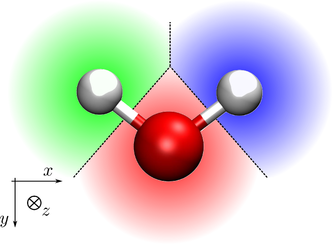
Figure 1: Cartoon of Voronoi-based density partitioning for a water molecule (rendered with VMD humphrey1996vmd ). Dashed lines delineate the partition boundaries. The axis system illustrates the orientation of the water molecule’s global frame for the calculations presented in Sec. III.1: aligned in the $xy$ plane with the oxygen atom pointing toward the $y$ axis.

Note that the Voronoi model contains no free parameter—the free-atom radii being applied without prior fitting. Though the model hardly reproduces any of the reference MTP coefficients, it provides a qualitative evaluation of the coefficients. In particular, the baseline model reproduces elementary symmetries of the system that are entirely determined by the geometry, e.g., a planar molecule cannot generate an orthogonal dipole moment.

While we compute Eqns. 7, 8, and 9 in Cartesian coordinates, we subsequently convert them to their spherical counterparts $Q_{\kappa m}$, where $\kappa$ denotes the rank (e.g., $\kappa=0$ for monopoles) and $m$ indexes the (real) component of the MTP (see Stone stone2013theory for more details). Given a molecular structure, we estimate for each atom the baseline property $p^{\rm Vor}=\{Q_{00},Q_{1m},Q_{2m}\}$, where $m$ runs over the $2\kappa+1$ elements of an MTP of order $\kappa$.

II.4 Molecular dataset

To refine atomic properties beyond the baseline prediction, we train the transferable ML algorithm on $2,896$ neutral molecules obtained from the Ligand.Info database grotthuss2004ligand , totaling 82.1 kilo atoms. Atoms have been segregated between training and prediction pools randomly. The database provides three-dimensional coordinates of small, organic molecules. We focus exclusively on a subset of neutral molecules that include elements H, C, N, O, S, F, and Cl.

III Results

III.1 Voronoi-based baseline evaluation

To illustrate the applicability of the Voronoi-based baseline evaluation of MTP coefficients, we compare its prediction with the reference MTP coefficients obtained from ab initio methods. Given that MTPs are inherently axis-system dependent (apart from the monopole), we first describe the global frame used for the water molecule in Fig. 1. Inherent symmetries of the geometry impose some coefficients to be zero, e.g., there can be no dipole moment along the $x$ or $z$ directions due to the molecule’s $C_{2v}$ symmetry. While the Voronoi-baseline does not even qualitatively reproduce the non-zero coefficients—due to the method not entailing any prior parametrization—its ability to impose the right symmetry is very desirable. The same kind of behavior is also shown for a carbon atom on benzene, or the carbonyl oxygen of formic acid in Tab. 1. For comparison, Tab. 1 also shows already the corresponding ML augmented MTP result. As such, the baseline recovers an important aspect of the underlying symmetry, which the augmenting ML model no longer needs to account for.

	$Q_{00}$	$Q_{10}$	$Q_{11c}$	$Q_{11s}$	$Q_{20}$	$Q_{21c}$	$Q_{21s}$	$Q_{22c}$	$Q_{22s}$
water oxygen
Vor	0.04	0	0	-0.12	0.43	0	0	-0.21	0.01
$\Delta$-ML	-0.13	-0.01	-0.02	0	0.16	-0.03	0.04	-0.18	0
Ref	-0.39	0	0.01	-0.40	-0.92	0	0	0.45	0
formic acid carbonyl oxygen
Vor	0.01	0	0	0	0.08	0	0	0	0
$\Delta$-ML	-0.35	-0.30	-0.03	0.03	0.55	0.10	-0.04	-0.10	0.15
Ref	-0.45	-0.10	-0.15	0	0.38	0.13	0	-0.32	0
benzene carbon
Vor	0.01	-0.01	0.01	0	-0.01	0	0	0.07	0.01
$\Delta$-ML	-0.10	-0.04	-0.10	-0.09	-0.73	-0.24	0.19	0.17	-0.05
Ref	-0.03	0	0	0	-0.65	0	0	-0.14	0

Table 1: MTP coefficients of oxygen in water (see Fig. 1) and in the carbonyl bond of formic acid, as well as the MTPs of carbon in benzene. “Vor,” “$\Delta$-ML,” and “ref” correspond to the Voronoi-based property evaluation, the delta-learned prediction across chemical compound space (see the $\Delta$-ML-85 model below), and the ab initio data, respectively. All coefficients are expressed in units $e$Å^l, where $l$ is the MTP’s rank. The comparatively low accuracy of the $\Delta$-ML model for water is rationalized in the main text.

III.2 $\Delta$-ML MTP model trained and tested across chemical space

In principle, the above-mentioned Coulomb matrix encodes enough chemistry to train all chemical elements. Memory limitations of the kernel-ridge regression, however, make atom-type specific models better tractable. We now investigate the $\Delta$-ML model’s capabilities to predict MTP coefficients across chemical space, one for each of those chemical elements that are most frequent in small, organic molecules (see above). The ML model has been trained on various fractions of the considered dataset’s 82 kilo atoms.

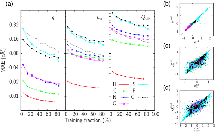
Figure 2: (a) Mean absolute prediction error (MAE) as a function of training set percentage of an 82k-atom database obtained from neutral molecules. MAEs are given in $e$Å^l units with $l$ being the MTP rank. Errors correspond to MTP $\Delta$-ML model predictions for individual components of atomic monopole, dipole, and quadrupole moments shown in left, mid, and right-hand side panel, respectively, for all elements present. Scatter correlation plots for all components of (b) monopoles, (c) dipoles, and (d) quadrupoles, as predicted with the $\Delta$-ML-85 model. Colors correspond to the atom legend in (a). The outliers in the monopole correlation curve correspond to sulfur-oxide groups (see main text).

Fig. 2 (a) displays error saturation curves for individual chemical elements. These monotonically decaying learning curves are presented as a function of training size of the dataset, where the predicted mean absolute error (MAE) is calculated across the remaining atoms not included in the training set. The finding of monotonically decreasing error with training set size represents numerical evidence for a crucial feature of the supervised-learning working hypothesis: The accuracy of the $\Delta$-ML model of MTPs improves as more data is being added. Monopole coefficients have the fastest learning rate, quickly reaching MAE between $0.1~{}e$ and $0.01~{}e$ for all elements. Differences between elements are simply due to their relative frequency in the data base. More specifically, since hydrogens and carbons predominate in small organic molecules they provide much larger training sets, and consequently more accurate ML models when measured in terms of percentage of training data being used. The scatter correlation plot between predicted and reference monopoles for each element is given in Fig. 2 (b) for the largest training fraction used: 85% (denoted “$\Delta$-ML-85”), the exception being the hydrogen $\Delta$-ML model trained on only 75% of the dataset given its converged accuracy. The monopoles modeled by $\Delta$-ML-85 reach high Pearson correlation coefficients: $R^{2}\approx 97\%$, except F and Cl, for which $R^{2}=17\%$ and $68\%$, respectively. Such poor performance is explained by the small size training data set available for these elements. The outliers in the monopole scatter plot (Fig. 2 (b)) correspond to sulfur-oxide groups. Also here, the few samples of these groups in the training set results in significant prediction errors.

Predicted dipoles show a MAE across elements between $0.02~{}e$Å and $0.15~{}e$Å, depending on training set size. The heterogeneity of the chemical environments of the elements is reflected in the ML-model’s performance. The $\Delta$-ML dipole moments of hydrogens are extremely accurate—most likely due to hydrogens showing weak overall MTP moments and due to their repeating saturating bonding pattern. By contrast, carbon atoms, albeit being nearly as frequent as hydrogens in the database, have MTP ML models with significantly larger MAE. We rationalize the $\Delta$-ML’s relative difficulty to predict this element by the large chemical variety carbon exhibits, i.e., strongly varying hybridization states and possible bonding with all other elements. Also note the reversal of the relative offset of the F and Cl learning curves as one proceeds from monopole to dipole moments, despite the fact that there are roughly twice as many Cl as F atoms in the data base. This effect is possibly due to chlorine’s larger polarizability, which implies that the chemical environment of the atom plays a more important role for the dipole-moment, turning the ML-based modeling into a higher-dimensional and thereby more challenging statistical-learning problem. Such effects, however, can only fully be explained through an in-depth study with significantly larger data sets. The scatter plot for predicted versus reference dipole moments is shown for all elements in Fig. 2 (c) for $\Delta$-ML-85. Clearly, the correlation is worse in comparison to monopoles ($R^{2}\approx 50\%$), which is in line with what one would expect for a more complex vectorial quantity.

Of all MTPs considered, quadrupoles represent the most complex and challenging property. Not surprisingly, the resulting ML models yield the largest MAE for our training set: between $0.02~{}e$Ų and $0.30~{}e$Ų depending on training set size. The spread of MAEs across elements is strikingly more pronounced. Nevertheless, we find a larger correlation coefficient compared to dipoles: $R^{2}\approx 65\%$, see Fig. 2 (c) and (d). Note that the Cl/F accuracy reversal with respect to the monopole model is also manifested for the $\Delta$-ML MTP model of this rank.

III.3 $\Delta$-ML MTP vs ML MTP model

			MAE [$e$Ål]
	# atoms		$q$		$\mu_{\alpha}$		$Q_{\alpha\beta}$
	training ($N_{t}$)	prediction	ML-85	$\Delta$-ML-85	ML-85	$\Delta$-ML-85	ML-85	$\Delta$-ML-85
H	28,822	9,607	0.01	0.01	0.03	0.01	0.04	0.02
C	24,356	4,297	0.01	0.01	0.05	0.05	0.18	0.09
N	4,054	715	0.02	0.02	0.09	0.05	0.26	0.15
O	6,134	1,082	0.02	0.02	0.08	0.04	0.22	0.12
F	363	63	0.03	0.09	0.04	0.05	0.14	0.11
S	1,542	272	0.05	0.05	0.12	0.09	0.31	0.20
Cl	739	130	0.03	0.06	0.11	0.10	0.28	0.26
	66,010	16,166	0.02	0.04	0.08	0.06	0.20	0.13

Table 2: MAE for each chemical element and MTP rank of the ML-85 and $\Delta$-ML-85 transferable models (neutral molecules), corresponding to an 85% training-set size for all elements but H (only 75%). The last lines averages over all chemical elements. The second column denotes the number of molecules for which the MTP moments have been predicted.

We have compared the relative improvement gained when combining the ML with the baseline evaluation from the Voronoi scheme. Tab. 2 compares MAEs decomposed by chemical element for the prediction with 85$\%$ training fraction both with (i.e., “$\Delta$-ML-85”) and without (i.e., “ML-85”) prior Voronoi baseline evaluation. The table also specifies the number of atoms involved in the prediction pool (i.e., outside the training fraction). While the Voronoi scheme does nothing to improve monopoles (for F and Cl it even worsens the prediction) it is increasingly helpful as we move to dipoles (with negligible change for F and Cl), and quadrupoles (with small improvement for F and Cl). We stress that the observed trends for F and Cl should be interpreted with utmost caution since their frequency in the database is very small (363 and 739). The lack of improvement for monopoles stems directly from the Voronoi scheme’s strategy: Merely encoding symmetries, only higher MTP moments can benefit from the absence of a number of components that are forbidden by the underlying geometry. For fixed training size, the MAE is roughly halved for quadrupoles when using the delta learning procedure, compared to the standard ML methodology.

All results discussed so far refer to ML models of atomic MTPs in neutral molecules. For positively and negatively charged compounds we have found ML models to yield very similar trends and accuracy (data not shown).

IV Validation

To assess the introduced MTP model’s applicability we have used predicted electrostatic coefficients to evaluate intermolecular interaction energies in molecular dimers and organic crystals. To do this, we accounted only for static MTP electrostatics and many-body dispersion (MBD) interactions,

$$E_{\rm vdW}\approx E_{\rm MTP}+E_{\rm MBD},$$ (12)

neglecting induction, penetration, and repulsion terms. A short description of the MBD formalism is provided in the next paragraph. As discussed above, our MTP and MBD-models also represent approximations in the form of the $\Delta$-ML model and dipole-dipole-manybody expansion, respectively. To better gauge the effect of the introduced MTP-ML model, we also compare to vdW energy predictions using quantum-mechanically (QM) derived MTPs.

Common approximations in the exchange-correlation potential used in density functional theory lead to inadequate predictions of dispersion interactions. This has motivated the development of a number of dispersion-corrected methods. We hereby rely on the method developed by Tkatchenko and coworkers MBD , in which free-atom polarizabilities are first scaled according to their close environment following a partitioning of the electron density. The many-body dispersion up to infinite order (in the dipole approximation) is then obtained by diagonalizing the Hamiltonian of a system of coupled quantum harmonic oscillators, thereby coupling the scaled atomic polarizabilities at long range. The importance of many-body effects and accuracy of the method has been demonstrated on a large variety of systems MBD . Later, a classical approximation relaxed the requirement for an electron density, using instead a physics-based approach to estimate how atomic polarizabilities needed to be scaled based on a Voronoi partitioning bereau2014toward .

IV.1 Molecular dimers

To gauge the accuracy of the electrostatics alone, we compare the electrostatic componenent of reference symmetry adapted perturbation theory (SAPT) results hesselmann2011comparison ; lao2014symmetry to the corresponding intermolecular components derived either from QM MTPs or from the $\Delta$-ML-MTP model. Fig. 3 displays the correlation plot between the two model MTP electrostatics calculations and SAPT for the S22 dimersjurevcka2006benchmark at different intermolecular distances grafova2010comparative ; hesselmann2011comparison ; lao2014symmetry . The plot confirms that both MTP models generally underestimate the electrostatic SAPT component of the interaction energies, presumably due to a lack of penetration effects. Encouragingly, as the intermolecular distance is increased, the MTP predictions systematically recede to the perfect correlation line.

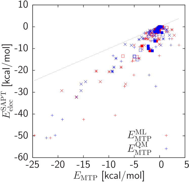
Figure 3: Scatter plot between reference energy components from SAPT and computed electrostatics from either quantum-mechanical coefficients, $E_{\rm MTP}^{\rm QM}$, or the universal $\Delta$-ML-85 MTP model, $E_{\rm MTP}^{\rm ML}$, for intermolecular dimers in the S22x5 dataset grafova2010comparative . Dimers closer than the equilibrium distance (i.e., factor 0.9) were systematically excluded. Symbols correspond to different distance factors that multiply the equilibrium distance: 0.9 (plus sign), 1.0 (cross), 1.2 (star), 1.5 (open square), and 2.0 (filled square). The straight line corresponds to ideal correlation.

Not all errors are distributed uniformly across compounds. Fig. 4 compares the MTP energy contributions $E_{\rm MTP}^{\rm QM}$ and $E_{\rm MTP}^{\rm ML}$, as well as reference SAPT data for each molecular dimer of the S22 dataset (i.e., at their equilibrium distance). We find good correlations between the QM and MTP models, though we note a number of qualitative discrepancies. In particular, the ML model fails to reproduce the attractive nature of the electrostatic interaction for the water and ammonia dimers. Presumably, the model fails to predict their coefficients due to the molecules’ unique chemical composition: the ML model relies on interpolations across the trained molecules, of which some must be chemically similar to the new compound. Larger molecules are less problematic because similarities between chemical fragments occur far more frequently. We do find systematic deviations between the MTP energies and the SAPT reference electrostatic data for strongly hydrogen-bonding compounds, for which penetration effects stone2013theory become significant.

Figure 4: Intermolecular static electrostatic energy contribution for each dimer of the S22 dataset, for coefficients parametrized from quantum-mechanical calculations, $E_{\rm MTP}^{\rm QM}$, and the transferable ML model $\Delta$-ML-85, $E_{\rm MTP}^{\rm ML}$. Electrostatic energies from reference SAPT calculations are also provided lao2014symmetry .

We have calculated molecular dimer energies corresponding to various datasets for which high-level quantum-chemistry numbers have previously been published. We have considered the following databases: S22 jurevcka2006benchmark , S22x5 grafova2010comparative , S66 and S66x8 rezac2011s66 , SCAI berka2009representative , and X40 and X40x10 rezac2012benchmark . All MTP coefficients have been predicted using the $\Delta$-ML-85 model (see Fig. 2 and Tab. 2). We only considered dimers made up of the chemical elements H, C, O, N, S, F, and Cl, keeping 992 out of over 1,300 vdW dimers.

Figure 5: Correlation plot between reference vdW energies, $E_{\rm ref}$, and energies predicted from the classical many-body dispersion method with static electrostatics, the latter parametrized from the $\Delta$-ML-85 model, $E_{\rm MTP}^{\rm ML}+E_{\rm MBD}$. The inset corresponds to the two charged-charged side-chain interactions of the SCAI database. The present lack of repulsion, induction, and penetration effects is at cause for the outliers.

Fig. 5 contrasts the scatter correlation between reference intermolecular energies, $E_{\rm ref}$, and the sum of many-body dispersion and ML-predicted MTP electrostatics, $E_{\rm MTP}^{\rm ML}+E_{\rm MBD}$. The mean-absolute error of all intermolecular estimates using the MTPs from individual quantum-chemistry calculations bereau2014toward and the ML predictions amount to 2.36 and 2.19 kcal/mol, respectively. In other words, the ML MTP prediction is on par with MTPs derived from explicit electron densities generated by computationally demanding quantum-chemistry calculations. Interactions between charged-charged amino acids of the SCAI database are reasonably well reproduced (see insets of Fig. 5), pointing to the robustness of the method not only for neutral compounds, but also charged species.

IV.2 Benzene crystal

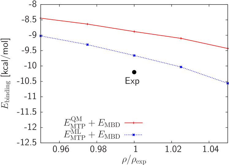
Figure 6: Cohesive binding energy of the benzene crystal as a function of the ratio of densities, $\rho/\rho_{\rm exp}$. Both models for intermolecular energies are presented: $E_{\rm MTP}^{\rm QM}+E_{\rm MBD}$ and $E_{\rm MTP}^{\rm ML}+E_{\rm MBD}$. The experimental value is shown explicitly (black dot) schweizer2006quantum .

Increasingly accurate and fast methods provide the means for crystal structure prediction of organic compounds bardwell2011towards , to the point of ranking polymorphs of molecular crystals marom2013many ; reilly2014role . Moving toward a condensed-phase system, we have also evaluated the cohesive binding energy predictions of a molecular benzene crystal. Following previous workmeijer1996density ; tapavicza2007weakly , we have computed the binding energy for different ratios of the unit-cell density with respect to the experimental density schweizer2006quantum , $\rho/\rho_{\rm exp}$. Isotropic density scalings were performed without further optimization, and the binding energy included interactions with the neighboring unit cells, as discussed in our previous publication bereau2014toward . Fig. 6 features the MTP and MBD based vdW estimates of cohesive energy as a function of density. Again, we compare the resulting numbers once using the $\Delta$-ML-predicted MTP electrostatics, combined with MBD, and once using the QM MTP model combined with MBD. We find very good agreement between the two methods, validating here as well the ML model. Coincidentally, the two methods yield cohesive binding energies in good agreement with the experimental value. The lack of repulsive interactions prohibits a further increase in energy as $\rho$ gets larger bereau2014toward .

V Conclusion

We have introduced machine-learning models for electrostatic multipoles (MTPs) of H, C, O, N, S, F, and Cl atom types. The models have been trained on atomic multipole coefficients of small organic molecules evaluated using first principles calculations. Neutral, cationic, and anionic molecular states were treated with separate models. The model yields highly accurate MTPs for H, reasonable performance for C, N, O, and significant errors for S, F and Cl due to their sparsity in the training set.

Focusing on the intermolecular S22 dimer dataset, MTP energies show good correlation between the coefficients parametrized from ML and individual quantum-chemistry calculations. A comparison with reference electrostatic interactions from symmetry-adapted perturbation theory (SAPT) is satisfactory for large intermolecular separations, and impaired by the lack of penetration effects at short distances. Furthermore, MTPs from the ML model have been combined with a classical many-body dispersion potential to estimate intermolecular energies of nearly 1,000 molecular dimers as well as the cohesive energy of the benzene crystal. The results show that the ML model retains overall a similar accuracy compared to calculations with the MTPs parametrized from individual quantum-chemical calculations.

The $\Delta$-ML approach, which augments a physics-based baseline model by a ML model, has proven to be useful to more efficiently train vector and tensor quantities. Incorporation of molecular symmetries via the Voronoi partitioning of the charge density, included in the baseline model, is at the heart of this improvement.

The proposed models alleviate the need for quantum-chemistry calculations for every single molecule/molecular conformation in a perturbative evaluation of intermolecular interactions, bringing us one step forward toward the task of automated parametrizations of accurate state-independent and transferable force fields.

VI Acknowledgments

We thank Andreas Hesselmann and John M. Herbert for kindly providing the SAPT reference energies, as well as Aoife Fogarty and Markus Meuwly for critical reading of the manuscript. OAvL acknowledges funding from the Swiss National Science foundation (No. PP00P2_138932). This research used resources of the Argonne Leadership Computing Facility at Argonne National Laboratory, which is supported by the Office of Science of the U.S. DOE under contract DE-AC02-06CH11357.

References

- (1) P. W. Atkins and J. de Paula, Physical Chemistry. Wiley-VCH, 2013.
- (2) J. N. Israelachvili, Intermolecular and Surface Forces. Academic Press, 1985.
- (3) G. Wedler, Lehrbuch der Physikalischen Chemie. Wiley-VCH, 1997.
- (4) W. L. Jorgensen, D. S. Maxwell, and J. Tirado-Rives, “Development and testing of the opls all-atom force field on conformational energetics and properties of organic liquids,” J. Am. Chem. Soc., vol. 118, no. 45, pp. 11225–11236, 1996.
- (5) A. Stone, The theory of intermolecular forces. Oxford University Press, 2013.
- (6) C. Kramer, A. Spinn, and K. R. Liedl, “Charge anisotropy: Where atomic multipoles matter most,” J. Chem. Theory Comput., vol. 10, no. 10, pp. 4488–4496, 2014.
- (7) J.-P. Piquemal, H. Chevreau, and N. Gresh, “Toward a separate reproduction of the contributions to the hartree-fock and dft intermolecular interaction energies by polarizable molecular mechanics with the sibfa potential,” J. Chem. Theory Comput., vol. 3, no. 3, pp. 824–837, 2007.
- (8) N. Gresh, G. A. Cisneros, T. A. Darden, and J.-P. Piquemal, “Anisotropic, polarizable molecular mechanics studies of inter-and intramolecular interactions and ligand-macromolecule complexes. a bottom-up strategy,” J. Chem. Theory Comput., vol. 3, no. 6, pp. 1960–1986, 2007.
- (9) M. S. Gordon, Q. A. Smith, P. Xu, and L. V. Slipchenko, “Accurate first principles model potentials for intermolecular interactions,” Annual review of physical chemistry, vol. 64, pp. 553–578, 2013.
- (10) J. W. Ponder, C. Wu, P. Ren, V. S. Pande, J. D. Chodera, M. J. Schnieders, I. Haque, D. L. Mobley, D. S. Lambrecht, R. A. DiStasio Jr, M. Head-Gordon, G. N. I. Clark, M. E. Johnson, and T. Head-Gordon, “Current status of the amoeba polarizable force field,” J. Phys. Chem. B, vol. 114, no. 8, pp. 2549–2564, 2010.
- (11) T. Bereau, C. Kramer, and M. Meuwly, “Leveraging symmetries of static atomic multipole electrostatics in molecular dynamics simulations,” J. Chem. Theory Comput., vol. 9, no. 12, pp. 5450–5459, 2013.
- (12) M. W. Lee, J. K. Carr, M. Göllner, P. Hamm, and M. Meuwly, “2d ir spectra of cyanide in water investigated by molecular dynamics simulations,” J. Chem. Phys., vol. 139, no. 5, p. 054506, 2013.
- (13) P.-A. Cazade, T. Bereau, and M. Meuwly, “Computational two-dimensional infrared spectroscopy without maps: N-methylacetamide in water,” J. Phys. Chem. B, vol. 118, no. 28, pp. 8135–8147, 2014.
- (14) S. Jakobsen, T. Bereau, and M. Meuwly, “Multipolar force fields and their effects on solvent dynamics around simple solutes,” J. Phys. Chem. B, 2015.
- (15) C. Cortes and V. Vapnik, “Support-vector networks,” Machine learning, vol. 20, no. 3, pp. 273–297, 1995.
- (16) K. Muller, S. Mika, G. Ratsch, K. Tsuda, and B. Scholkopf, “An introduction to kernel-based learning algorithms,” Neural Networks, IEEE Transactions on, vol. 12, no. 2, pp. 181–201, 2001.
- (17) B. Schölkopf and A. J. Smola, Learning with kernels: Support vector machines, regularization, optimization, and beyond. MIT press, 2002.
- (18) I. H. Witten and E. Frank, Data Mining: Practical machine learning tools and techniques. Morgan Kaufmann, 2005.
- (19) B. G. Sumpter and D. W. Noid, “Potential energy surfaces for macromolecules. a neural network technique,” Chem. Phys. Lett., vol. 192, no. 5–6, pp. 455 – 462, 1992.
- (20) B. K. Rai and G. A. Bakken, “Fast and accurate generation of ab initio quality atomic charges using nonparametric statistical regression,” J. Comput. Chem., vol. 34, no. 19, pp. 1661–1671, 2013.
- (21) M. V. Ivanov, M. R. Talipov, and Q. K. Timerghazin, “Genetic algorithm optimization of point charges in force field development: Challenges and insights,” The Journal of Physical Chemistry A, 2015.
- (22) C. M. Handley, G. I. Hawe, D. B. Kell, and P. L. Popelier, “Optimal construction of a fast and accurate polarisable water potential based on multipole moments trained by machine learning,” Phys. Chem. Chem. Phys., vol. 11, no. 30, pp. 6365–6376, 2009.
- (23) M. J. Mills and P. L. Popelier, “Polarisable multipolar electrostatics from the machine learning method kriging: an application to alanine,” Theoretical Chemistry Accounts, vol. 131, no. 3, pp. 1–16, 2012.
- (24) T. Bereau and O. A. von Lilienfeld, “Toward transferable interatomic van der waals interactions without electrons: The role of multipole electrostatics and many-body dispersion,” J. Chem. Phys., vol. 141, no. 3, p. 034101, 2014.
- (25) K.-R. Müller, S. Mika, G. Rätsch, K. Tsuda, and B. Schölkopf, “An introduction to kernel-based learning algorithms,” IEEE Transactions on Neural Networks, vol. 12, no. 2, pp. 181–201, 2001.
- (26) T. Hastie, R. Tibshirani, and J. Friedman, The Elements of Statistical Learning: data mining, inference and prediction. Springer series in statistics, New York, N.Y.: Springer, 2001.
- (27) B. Schölkopf, A. Smola, and K.-R. Müller, “Nonlinear component analysis as a kernel eigenvalue problem,” Neural computation, vol. 10, no. 5, pp. 1299–1319, 1998.
- (28) R. Ramakrishnan, P. Dral, M. Rupp, and O. A. von Lilienfeld, “Big data meets quantum chemistry approximations: The -Machine Learning approach,” 2015. http://arxiv.org/abs/1503.04987.
- (29) M. Rupp, A. Tkatchenko, K.-R. Müller, and O. A. von Lilienfeld, “Fast and accurate modeling of molecular atomization energies with machine learning,” Phys. Rev. Lett., vol. 108, no. 5, p. 058301, 2012.
- (30) O. A. von Lilienfeld, R. Ramakrishnan, M. Rupp, and A. Knoll, “Fourier series of atomic radial distribution functions: A molecular fingerprint for machine learning models of quantum chemical properties,” Int. J. Quantum Chem., 2015. http://arxiv.org/abs/1307.2918.
- (31) K. Hansen, G. Montavon, F. Biegler, S. Fazli, M. Rupp, M. Scheffler, O. A. von Lilienfeld, A. Tkatchenko, and K.-R. Müller, “Assessment and validation of machine learning methods for predicting molecular atomization energies,” J. Chem. Theory Comput., vol. 9, no. 8, pp. 3404–3419, 2013.
- (32) R. Ramakrishnan and O. A. von Lilienfeld, “Many molecular properties from one kernel in chemical space,” CHIMIA, 2015.
- (33) Y. Zhao and D. G. Truhlar, “Exploring the limit of accuracy of the global hybrid meta density functional for main-group thermochemistry, kinetics, and noncovalent interactions,” J. Chem. Theory Comput., vol. 4, no. 11, pp. 1849–1868, 2008.
- (34) T. H. Dunning Jr, “Gaussian basis sets for use in correlated molecular calculations. i. the atoms boron through neon and hydrogen,” J. Chem. Phys., vol. 90, no. 2, pp. 1007–1023, 1989.
- (35) M. J. Frisch, G. W. Trucks, H. B. Schlegel, G. E. Scuseria, M. A. Robb, J. R. Cheeseman, G. Scalmani, V. Barone, B. Mennucci, G. A. Petersson, H. Nakatsuji, M. Caricato, X. Li, H. P. Hratchian, A. F. Izmaylov, J. Bloino, G. Zheng, J. L. Sonnenberg, M. Hada, M. Ehara, K. Toyota, R. Fukuda, J. Hasegawa, M. Ishida, T. Nakajima, Y. Honda, O. Kitao, H. Nakai, T. Vreven, J. A. Montgomery, Jr., J. E. Peralta, F. Ogliaro, M. Bearpark, J. J. Heyd, E. Brothers, K. N. Kudin, V. N. Staroverov, R. Kobayashi, J. Normand, K. Raghavachari, A. Rendell, J. C. Burant, S. S. Iyengar, J. Tomasi, M. Cossi, N. Rega, J. M. Millam, M. Klene, J. E. Knox, J. B. Cross, V. Bakken, C. Adamo, J. Jaramillo, R. Gomperts, R. E. Stratmann, O. Yazyev, A. J. Austin, R. Cammi, C. Pomelli, J. W. Ochterski, R. L. Martin, K. Morokuma, V. G. Zakrzewski, G. A. Voth, P. Salvador, J. J. Dannenberg, S. Dapprich, A. D. Daniels, . Farkas, J. B. Foresman, J. V. Ortiz, J. Cioslowski, and D. J. Fox, “Gaussian 09, revision a. 02, gaussian,” Inc., Wallingford, CT, vol. 200, 2009.
- (36) B. R. Brooks, C. L. Brooks, A. D. MacKerell, L. Nilsson, R. J. Petrella, B. Roux, Y. Won, G. Archontis, C. Bartels, S. Boresch, A. Caflisch, L. Caves, Q. Cui, A. Dinner, M. Feig, S. Fischer, J. Gao, M. Hodoscek, W. Im, K. Kuczera, T. Lazaridis, J. Ma, V. Ovchinnikov, E. Paci, R. Pastor, C. Post, J. Pu, M. Schaefer, B. Tidor, R. Venable, H. Woodcock, X. Wu, W. Yang, D. York, and M. Karplus, “Charmm: the biomolecular simulation program,” J. Comput. Chem., vol. 30, no. 10, pp. 1545–1614, 2009.
- (37) T. Bereau, C. Kramer, F. W. Monnard, E. S. Nogueira, T. R. Ward, and M. Meuwly, “Scoring multipole electrostatics in condensed-phase atomistic simulations,” J. Phys. Chem. B, vol. 117, no. 18, pp. 5460–5471, 2013.
- (38) https://github.com/tbereau/mbvdw.
- (39) X. Chu and A. Dalgarno J. Chem. Phys., vol. 121, p. 4083, 2004.
- (40) O. A. von Lilienfeld and A. Tkatchenko, “Two-and three-body interatomic dispersion energy contributions to binding in molecules and solids,” J. Chem. Phys., vol. 132, p. 234109, 2010.
- (41) A. Okabe, B. Boots, K. Sugihara, and S. N. Chiu, Spatial tessellations: concepts and applications of Voronoi diagrams, vol. 501. Wiley.com, 2009.
- (42) W. Humphrey, A. Dalke, and K. Schulten, “Vmd: visual molecular dynamics,” J. Mol. Graph. Model., vol. 14, no. 1, pp. 33–38, 1996.
- (43) M. v. Grotthuss, G. Koczyk, J. Pas, L. S. Wyrwicz, and L. Rychlewski, “Ligand. info small-molecule meta-database,” Combinatorial chemistry & high throughput screening, vol. 7, no. 8, pp. 757–761, 2004.
- (44) A. Tkatchenko, R. A. DiStasio Jr., R. Car, and M. Scheffler, “Accurate and efficient method for many-body van der waals interactions,” Phys. Rev. Lett., vol. 108, p. 236402, 2012.
- (45) A. Hesselmann, “Comparison of intermolecular interaction energies from sapt and dft including empirical dispersion contributions,” The Journal of Physical Chemistry A, vol. 115, no. 41, pp. 11321–11330, 2011.
- (46) K. U. Lao and J. M. Herbert, “Symmetry-adapted perturbation theory with kohn-sham orbitals using non-empirically tuned, long-range-corrected density functionals,” J. Chem. Phys., vol. 140, no. 4, p. 044108, 2014.
- (47) P. Jurečka, J. Šponer, J. Černỳ, and P. Hobza, “Benchmark database of accurate (MP2 and CCSD (T) complete basis set limit) interaction energies of small model complexes, DNA base pairs, and amino acid pairs,” Phys. Chem. Chem. Phys., vol. 8, no. 17, pp. 1985–1993, 2006.
- (48) L. Gráfová, M. Pitoňák, J. Řezáč, and P. Hobza, “Comparative study of selected wave function and density functional methods for noncovalent interaction energy calculations using the extended s22 data set,” J. Chem. Theory Comput., vol. 6, no. 8, pp. 2365–2376, 2010.
- (49) J. Rezác, K. E. Riley, and P. Hobza, “S66: A well-balanced database of benchmark interaction energies relevant to biomolecular structures,” J. Chem. Theory Comput., vol. 7, no. 8, pp. 2427–2438, 2011.
- (50) K. Berka, R. Laskowski, K. E. Riley, P. Hobza, and J. Vondrášek, “Representative amino acid side chain interactions in proteins. a comparison of highly accurate correlated ab initio quantum chemical and empirical potential procedures,” J. Chem. Theory Comput., vol. 5, no. 4, pp. 982–992, 2009.
- (51) J. Řezáč, K. E. Riley, and P. Hobza, “Benchmark calculations of noncovalent interactions of halogenated molecules,” J. Chem. Theory Comput., vol. 8, no. 11, pp. 4285–4292, 2012.
- (52) W. B. Schweizer and J. D. Dunitz, “Quantum mechanical calculations for benzene dimer energies: Present problems and future challenges,” J. Chem. Theory Comput., vol. 2, no. 2, pp. 288–291, 2006.
- (53) D. A. Bardwell, C. S. Adjiman, Y. A. Arnautova, E. Bartashevich, S. X. Boerrigter, D. E. Braun, A. J. Cruz-Cabeza, G. M. Day, R. G. Della Valle, G. R. Desiraju, B. P. van Eijck, J. C. Facelli, M. B. Ferraro, D. Grillo, M. Habgood, D. W. M. Hofmann, F. Hofmann, K. V. J. Jose, P. G. Karamertzanis, A. V. Kazantsev, J. Kendrick, L. N. Kuleshova, F. J. J. Leusen, A. V. Maleev, A. J. Misquitta, S. Mohamed, R. J. Needs, M. A. Neumann, D. Nikylov, A. M. Orendt, R. Pal, C. C. Pantelides, C. J. Pickard, L. S. Price, S. L. Price, H. A. Scheraga, J. van de Streek, T. S. Thakur, S. Tiwari, E. Venuti, and I. K. Zhitkov, “Towards crystal structure prediction of complex organic compounds–a report on the fifth blind test,” Acta Crystallographica Section B: Structural Science, vol. 67, no. 6, pp. 535–551, 2011.
- (54) N. Marom, R. A. DiStasio, V. Atalla, S. Levchenko, A. M. Reilly, J. R. Chelikowsky, L. Leiserowitz, and A. Tkatchenko, “Many-body dispersion interactions in molecular crystal polymorphism,” Angewandte Chemie International Edition, vol. 52, no. 26, pp. 6629–6632, 2013.
- (55) A. M. Reilly and A. Tkatchenko, “Role of dispersion interactions in the polymorphism and entropic stabilization of the aspirin crystal,” Phys. Rev. Lett., vol. 113, no. 5, p. 055701, 2014.
- (56) E. J. Meijer and M. Sprik, “A density-functional study of the intermolecular interactions of benzene,” J. Chem. Phys., vol. 105, no. 19, pp. 8684–8689, 1996.
- (57) E. Tapavicza, I.-C. Lin, O. A. von Lilienfeld, I. Tavernelli, M. D. Coutinho-Neto, and U. Rothlisberger, “Weakly bonded complexes of aliphatic and aromatic carbon compounds described with dispersion corrected density functional theory,” J. Chem. Theory Comput., vol. 3, no. 5, pp. 1673–1679, 2007.