Abstract

p2poc is an add–on toolbox to the Matlab package pde2path. It is aimed at the numerical solution of infinite time horizon optimal control (OC) problems for parabolic systems of PDE over 1D or 2D spatial domains. The basic idea is to treat the OC problem via the associated canonical system in two steps. First we use pde2path to find branches of stationary solutions of the canonical system, also called canonical steady states (CSS). In a second step we use the results and the spatial discretization of the first step to calculate the objective values of time-dependent canonical paths ending at a CSS with the so called saddle point property. This is a (typically very high dimensional) boundary value problem (BVP) in time, which we solve by combining a modification of the BVP solver TOM with a continuation algorithm in the initial states. We explain the design and usage of the package via two example problems, namely the optimal management of a distributed shallow lake model, and of a semi-arid grazing system. Both show interesting bifurcations of so called patterned CSS, and in particular the latter also a variety of patterned optimal steady states. The package (library and demos) can be downloaded at www.staff.uni-oldenburg.de/hannes.uecker/pde2path.

1 Introduction

Denoting the state variable (vector) by $v=v(t,x)\in{\mathbb{R}}^{N}$, and the control by $k=k(t,x)\in{\mathbb{R}}$, we consider spatially distribute infinite time horizon optimal control (OC) problems of the form

$$V(v_{0}(\cdot)):=\max_{k(\cdot,\cdot)}J(v_{0}(\cdot),k(\cdot,\cdot)),\qquad J(v_{0}(\cdot),k(\cdot,\cdot)):=\int_{0}^{\infty}{\rm e}^{-\rho t}J_{ca}(v(t),k(t))\,{\rm d}t,$$ (1a)

where $$J_{ca}(v(\cdot,t),k(\cdot,t))=\frac{1}{|\Omega|}\int_{\Omega}J_{c}(v(x,t),k(x,t))\,{\rm d}x$$ (1b)

is the spatially averaged current value objective function, with the local current value $$J_{c}{:}{\mathbb{R}}^{N+1}{\rightarrow}{\mathbb{R}} \rho>0 v:\Omega\times[0,\infty)\rightarrow{\mathbb{R}}^{N}$$ a given function; is the discount rate, and fulfills a PDE of the form

$${\partial}_{t}v=-G_{1}(v,k):=D\Delta v+g_{1}(v,k),\quad v|_{t=0}=v_{0}.$$ (1c)

Here, $D\in{\mathbb{R}}^{N\times N}$ is a diffusion matrix, $\Delta={\partial}_{x_{1}}^{2}+\ldots+{\partial}_{x_{d}}^{2}$ is the Laplacian, and (1c) holds in a bounded domain $\Omega\subset{\mathbb{R}}^{d}$ with suitable boundary conditions (BC), where for simplicity we restrict to homogeneous Neumann ${\partial}_{\nu}v=0$, $\nu$ the outer normal. In applications, $J_{c}$ and $G_{1}$ of course often also depend on a number of parameters, which however for simplicity we do not display here.

Introducing the costates $\lambda:\Omega\times(0,\infty)\rightarrow{\mathbb{R}}^{N}$ and the (local current value) Hamiltonian

$${\cal H} ={\cal H}(v,\lambda,k)=J_{c}(v,k)+\lambda^{T}(D\Delta v+g_{1}(v,k)),$$ (2)

by Pontryagin’s Maximum Principle (see the references below) for $\tilde{{\cal H}}=\int_{0}^{\infty}{\rm e}^{-\rho t}{\overline{{\cal H}}}(t)\,{\rm d}t$ with the spatial integral

$${\overline{{\cal H}}}(t)=\int_{\Omega}{\cal H}(v(x,t),\lambda(x,t),k(x,t))\,{\rm d}x,$$ (3)

an optimal solution $(v,\lambda)$ (or equivalently $(v,k):\Omega\times[0,\infty)\rightarrow{\mathbb{R}}^{N+1})$) has to solve the canonical system (CS)

$${\partial}_{t}v ={\partial}_{\lambda}{\cal H}=D\Delta v+g_{1}(v,k),\quad v|_{t=0}=v_{0},$$ (4a)

$${\partial}_{t}\lambda =\rho\lambda-{\partial}_{v}{\cal H}=\rho\lambda+g_{2}(v,k)-D\Delta\lambda,$$ (4b)

where $$k=\operatornamewithlimits{argmax}_{\tilde{k}}{\cal H}(v,\lambda,\tilde{k})$$, which generally we assume to be obtained from solving

$${\partial}_{k}{\cal H}(v,\lambda,k) =0.$$ (4c)

The costates $\lambda$ also fulfill zero flux BC, and derivatives like ${\partial}_{v}{\cal H}$ etc are taken variationally, i.e., for ${\overline{{\cal H}}}$. For instance, for $N=1$ and $\Phi(v,\lambda):=\lambda\Delta v$ we have ${\overline{\Phi}}(v,\lambda)=\int_{\Omega}\lambda\Delta v\,{\rm d}x=\int_{\Omega}(\Delta\lambda)v\,{\rm d}x$ by Gauß’ theorem, hence $\delta_{v}{\overline{\Phi}}(v,\lambda)[h]=\int(\Delta\lambda)h\,{\rm d}x$, and by the Riesz representation theorem we identify $\delta_{v}{\overline{\Phi}}(v,\lambda)$ and hence ${\partial}_{v}\Phi(v,\lambda)$ with the multiplier $\Delta\lambda$. ((4)c) typically applies and yields a unique solution $k$ under suitable concavity assumptions on ${\cal H}$, and in the absence of control constraints, see below.

In principle we want so solve (4) for $t\in[0,\infty)$, but in (4a) we have initial data for only half the variables, and in (4b) we have anti–diffusion, such that (4) is ill–posed as an initial value problem. For convenience we set

$$u(t,\cdot):=\begin{pmatrix}v(t,\cdot)\\ \lambda(t,\cdot)\end{pmatrix}:\Omega\rightarrow{\mathbb{R}}^{2N},$$ (5)

and write (4) as

$${\partial}_{t}u =-G(u,\eta):={\cal D}\Delta u+f(u),\text{ where }{\cal D}=\begin{pmatrix}D&0\\ 0&-D\end{pmatrix},\quad f(u)=\begin{pmatrix}g_{1}(u)\\ g_{2}(u)\end{pmatrix},$$ (6a)

and where $$\eta\in{\mathbb{R}}^{p} \rho {\partial}_{\nu}u=0$$ stands for parameters present, which for instance also includes the discount rate . Besides the boundary condition and the initial condition

$$v|_{t=0} =v_{0},$$ (6b)

we then impose the tranversality condition

$$\lim_{t\to\infty}{\rm e}^{-\rho t}u(t) =0.$$ (6c)

A solution $u$ of the canonical system (6) is called a canonical path, and an equilibrium of (6a) (which automatically fulfils (6c)) is called canonical steady state (CSS). With a slight abuse of notation we also call $(v,k)$ with $k$ given by (4d) a canonical path. See also, e.g., [GU15] for more formal definitions, further comments on the notions of optimal systems, and, e.g., the significance of the transversality condition (6c).

For general background on OC in a PDE setting see [Trö10] and the references therein, or specifically [RZ99a, RZ99b] and [AAC11, Chapter5] for Pontryagin’s Maximum Principle for OC problems for semilinear diffusive models. However, these works are in a finite time horizon setting, and often the objective function is linear in the control and there are control constraints, e.g., $k(x,t)\in K$ with some bounded interval $K$. Therefore $k$ is not obtained from the analogue of (4c), but rather takes the values from ${\partial}K$, which is often called bang control. In, e.g., [CPB12, ACKLT13], some specific models have been studied in this setting and a rather theoretical way, i.e., the focus is on deriving the canonical system and showing well-posedness and the existence of an optimal control. [ADS14] additionally contains numerical simulations for a finite time horizon control–constrained OC problem for a three species spatial predator-prey system, again leading to bang type controls. See also [NPS11] and the references therein for numerical methods for (finite time horizon) constrained parabolic optimal control problems.

Here we do not (yet) consider (active) control or state constraints, and no terminal time, but the infinite time horizon. Our models and method are motivated by [BX08, BX10], which also discuss Pontryagin’s Maximum Principle in this setting. We do not extend the theory, but rather consider (6) after a spatial discretization as a (large) ODE problem, and essentially treat this using the notations and ideas from [GCF⁺08], to give a numerical framework to calculate optimal solutions. Using the canonical system (4) we proceed in two steps, which can be seen as a variant of the “connecting orbit method”, see, e.g., [BPS01], and also §3 for further background and remarks on the related literature: first we compute (branches of) CSS, and second we compute canonical paths connecting to some CSS. This also means that we take a somewhat broader perspective than aiming at computing just one optimal control, given an initial condition $v_{0}$, which without further information is ill-posed anyway. Instead, our method aims to give a somewhat global picture by identifying the pertinent CSS and their respective domains of attraction.

(a) CSS branches.

We compute (approximate) CSS of (6), i.e., solutions $\hat{u}$ of

$$G(u,\eta)=0,$$ (7)

together with the BC. For this use the package pde2path [UWR14, DRUW14] to set up a FEM discretization of (7) as a continuation/bifurcation problem in one of the parameters, which we call $\eta$ again. This gives branches $\eta\mapsto\hat{u}(\eta)$ of solutions, which is in particular useful to possibly find several solutions $\hat{u}^{(l)}(\eta)$, $j=l,\ldots,m$ at fixed $\eta$. By computing the associated $J_{ca}(\hat{v}^{(l)},k^{(l)})$ we can identify which of these is optimal amongst the CSS. Given a CSS $\hat{u}$, for simplicity we also write $J_{ca}(\hat{u}):=J_{ca}(\hat{v}^{(l)},k^{(l)})$, and moreover, have

$$J(\hat{u})=J_{ca}(\hat{u})/\rho.$$ (8)

(b) Canonical paths.

In a second step (b), we calculate canonical paths ending at a CSS $\hat{u}$ (and often starting at the state values $\hat{v}_{0}$ of a different CSS $\hat{u}_{0}$), and the objective values of the canonical paths. For this we choose a truncation time $T$ and modify (6c) to the condition that $u(T)\in W_{s}(\hat{u})$ and near $\hat{u}$, where $W_{s}(\hat{u})$ denotes the stable manifold of $\hat{u}$. In practice, we approximate $W_{s}(\hat{u})$ by the stable eigenspace $E_{s}(\hat{u})$, and thus consider the BVP

$${\partial}_{t}u =-G(u),$$ (9a)

$$v|_{t=0} =v_{0},$$ (9b)

$$u(T) \in E_{s}(\hat{u})\text{ (and $\|u(T)-\hat{u}\|$ small)}.$$ (9c)

Using the spatial FEM discretizations, the implementation of $G$, and the results from the first step (a), if the mesh in the FEM consists of $n$ nodes, then $u(t)\in{\mathbb{R}}^{2Nn}$, and (9a) yields a system of $2Nn$ ODEs in the form (with a slight abuse of notation)

$$M\frac{\rm d}{{\rm d}t}u =-G(u),$$ (10a)

while the initial and transversality conditions become

$$v|_{t=0} =v_{0},$$ (10b)

$$\Psi(u(T)-\hat{u}) =0\text{ (and $\|u(T)-\hat{u}\|$ small)}.$$ (10c)

Here $M\in{\mathbb{R}}^{2Nn\times 2Nn}$ is the mass matrix of the FEM mesh, and $\Psi\in{\mathbb{R}}^{Nn\times 2Nn}$ defines the projection onto $E_{u}(\hat{u})$. Moreover, (10b) consists of $Nn$ initial conditions for the states, while the costates $\lambda$ (and hence the control $k$) are free. Thus, to have $2Nn$ BC altogether we need dim$E_{s}(\hat{u})=Nn$. On the other hand, we always have dim$E_{s}(\hat{u})\leq Nn$, see [GU15, Appendix A]. We define the defect

$$d(\hat{u}):={\rm dim}E_{s}(\hat{u})-Nn$$ (11)

and call a CSS $\hat{u}$ with $d(\hat{u})=0$ a CSS with the saddle–point property (SPP). At first sight it may appear that $d(\hat{u})$ depends on the spatial discretization, i.e., on the number of $n$ of nodes. However, $d(\hat{u})$ remains constant for finer and finer meshes, see [GU15, Appendix A] for further comments.

For $\hat{u}=(\hat{v},\hat{\lambda})$ with the SPP, and $\|v_{0}-\hat{v}\|$ sufficiently small, we may expect the existence of a solution $u$ of (10), which moreover can be found from a Newton loop for (10) with initial guess $u(t)\equiv\hat{u}$. On the other hand, for larger $\|v_{0}-\hat{v}\|$ a solution of (10) may not exist, or a good initial guess may be hard to find, and therefore we use a continuation process also for (10). In the simplest setting, assume that for some $\alpha\in[0,1]$ we have a solution $u_{\alpha}$ of (10) with (10b) replaced by

$$v(0)=\alpha v_{0}+(1-\alpha)\hat{v},$$ (12)

(e.g., $\alpha=0$ and $u\equiv\hat{u}$). We then increase $\alpha$ by some stepsize $\delta_{\alpha}$ and use $u_{\alpha}$ as initial guess for (10a), (10c) and (12), ultimately aiming at $\alpha=1$.

To actually solve (10a), (10c) and (12) we use TOM [MS02, MT04, MST09] (see also www.dm.uniba.it/~mazzia/mazzia/?page_id=433) in a version mtom which accounts for the mass matrix $M$ on the lhs of (10a). This predictor ($u_{\alpha}$) – corrector (mtom for $\alpha+\delta_{\alpha}$) continuation method corresponds to the “natural” parametrization of the continuation by $\alpha$, and is thus implemented in p2poc as iscnat (Initial State Continuation NATural). We also give the option to use a secant predictor

$$u^{j}(t)=u^{j-1}(t)+\delta_{\alpha}\tau(t),\quad\tau(t)=\bigl{(}u^{(j-1)}(t)-u^{(j-2)}(t)\bigr{)}/\|u^{(j-1)}(\cdot)-u^{(j-2)}(\cdot)\|_{2},$$ (13)

where $u^{j-2}$ and $u^{j-1}$ are the two previous steps. However, the corrector still works at fixed $\alpha$, in contrast to the arclength predictor–corrector iscarc described next.

It may happen that no solution of (10a), (10c) and (12) is found for $\alpha>\alpha_{0}$ for some $\alpha_{0}<1$, i.e., that the continuation to the intended initial states fails. In that case, often the BVP shows a fold in $\alpha$, and we use a modified continuation process, letting $\alpha$ be a free parameter and using a pseudo–arclength parametrization by $\sigma$ in the BC at $t=0$. Since mtom does not allow free parameters we add the dummy ODE $\dot{\alpha}=0$, and BCs at continuation step $j$,

$$\bigl{\langle}s,(u(0)-u^{(j-1)}(0)\rangle+s_{\alpha}(\alpha-\alpha^{(j-1)})=\sigma,$$ (14)

with $u^{(j-1)}(\cdot)$ the solution from the previous continuation step $j-1$, and $(s,s_{\alpha})\in{\mathbb{R}}^{2N}\times{\mathbb{R}}$ appropriately chosen with $\|(s,s_{\alpha})\|_{*}=1$, where $\|\cdot\|_{*}$ is a suitable norm in ${\mathbb{R}}^{2N+1}$, which may contain different weights of $v$ and $v_{\alpha}$. For $s=0$ and $s_{\alpha}=1$ we find iscnat with stepsize $\delta_{\alpha}=\sigma$ again. To get around folds we may use the secant

$$s:=\xi\bigl{(}u^{(j-1)}(0)-u^{(j-2)}(0)\bigr{)}/\|u^{(j-1)}(0)-u^{(j-2)}(0)\|_{2}\text{ and }s_{\alpha}=1-\xi$$

with small $\xi$, and also a secant predictor

$$(u^{j},\alpha^{j})^{\text{pred}}=(u^{j-1},\alpha^{j-1})+\sigma\tau$$ (15)

for $t\mapsto u^{j}(t)$ with

$$\tau=\xi\bigl{(}u^{(j-1)}(\cdot)-u^{(j-2)}(\cdot)\bigr{)}/\|u^{(j-1)}(\cdot)-u^{(j-2)}(\cdot)\|_{2}\text{ and }\tau_{\alpha}=1-\xi.$$ (16)

This essentially follows [GCF⁺08, §7.2], and is implemented in a routine iscarc (Initial State Continuation ARClength).

Finally, given $\hat{u}$, to calculate $\Psi$, at startup we solve the generalized adjoint eigenvalue problem

$${\partial}_{u}G(\hat{u})^{T}\Phi=\Lambda M\Phi$$ (17)

for the eigenvalues $\Lambda$ and (adjoint) eigenvectors $\Phi$, which also gives the defect $d(\hat{u})$ by counting the negative eigenvalues in $\Lambda$. If $d(\hat{u})=0$, then from $\Phi\in{\mathbb{C}}^{2Nn\times 2Nn}$ we generate a real base of $E_{u}(\hat{u})$ which we sort into the matrix $\Psi\in{\mathbb{R}}^{Nn\times 2Nn}$.

Acknowledgement. I thank D. Grass, ORCOS Wien, for introducing me to the field of optimal control over infinite time horizons, and for clarifying (and posing) many questions regarding the aim of software based on Pontryagin’s Maximum Principle for spatially distributed OC problems.

2 Examples and implementation details

2.1 The SLOC model

Following [BX08], in [GU15] we consider a model for phosphorus $P=P(t,x)$ in a shallow lake, and phosphate load $k=k(x,t)$ as a control, which in 0D, i.e., in the ODE setting, has analyzed in detail for instance in [KW10]. Here we explain how we set up the spatial so called Shallow Lake Optimal Control (SLOC) problem in p2poc, and refer to [GU15] for details about the modelling and the interpretation of results. The model reads

$$V(P_{0}(\cdot)):=\max_{k(\cdot,\cdot)}J(P_{0}(\cdot),k(\cdot,\cdot)),\qquad J(P_{0}(\cdot),k(\cdot,\cdot)):=\int_{0}^{\infty}{\rm e}^{-\rho t}J_{ca}(P(t),k(t)),\,{\rm d}t$$ (18a)

where $$J_{c}(P,k)=\ln(k)-\gamma P^{2}$$ is the local current value objective function,

$$J_{ca}(P(\cdot,t),k(\cdot,t))=\frac{1}{|\Omega|}\int_{\Omega}J_{c}(P(x,t),k(x,t))\!\,{\rm d}x$$ (18b)

is the spatially averaged current value objective function, and $$P$$ fulfills the PDE

$${\partial}_{t}P(x,t)=k(x,t)-bP(x,t)+\frac{P(x,t)^{2}}{1+P(x,t)^{2}}+D\Delta P(x,t),$$ (18c)

$${\partial}_{\nu}P(x,t)_{{\partial}\Omega}=0,\qquad P(x,t)_{t=0}=P_{0}(x),\quad x\in\Omega\subset{\mathbb{R}}^{d}.$$ (18d)

The parameter $b>0$ is the phosphor degradation rate, and $\gamma>0$ are ecological costs of the phosphor contamination $P$. One wants a low $P$ for ecological reasons, but for economical reasons a high phosphate load $k$, for instance from fertilizers used by farmers. Thus, the objective function consists of the concave increasing function $\ln(k)$, and the concave decreasing function $-\gamma P^{2}$. We consider two scenarios, namely

$$\text{ Scenario 1: }D=0.5,\rho=0.03,\gamma=0.5,b\in(0.5,0.8)\text{ (primary bif.~{}param.)},$$ (19)

$$\text{ Scenario 2: }D=0.5,\rho=0.3,b=0.55,\gamma\in(2.5,3.7)\text{ (primary bif.~{}param.)}.$$ (20)

With the co-state $q$ and local current value Hamiltonian

$${\cal H}(P,q,\lambda)=J_{c}(P,k)+q\bigl{[}k-bP+\frac{P^{2}}{1+P^{2}}+D\Delta P\bigr{]},$$ (21)

the canonical system for (18) becomes, with $\displaystyle k(x,t)=-\frac{1}{q(x,t)}$,

$${{\partial}_{t}}P(x,t) =k(x,t)-bP(x,t)+\frac{P(x,t)^{2}}{1+P(x,t)^{2}}+D\Delta P(x,t),$$ (22a)

$${\partial}_{t}q(x,t) =2\gamma P(x,t)+q(x,t)\left(\rho+b-\frac{2P(x,t)}{\left(1+P(x,t)^{2}\right)^{2}}\right)-D\Delta q(x,t),$$ (22b)

$${\partial}_{\nu}P(x,t)_{{\partial}\Omega} =0,\quad{\partial}_{\nu}q(x,t)_{{\partial}\Omega}=0,\qquad P(x,t)_{t=0}=P_{0}(x),\quad x\in\Omega.$$ (22c)

We now explain how to use p2poc to calculate CSS and canonical paths for (22). For this we discuss files from the demo directory slocdemo (except for obvious library files), assuming that slocdemo is in the same directory as the libraries p2plib, p2poclib and tom.

2.1.1 Basics of pde2path, and the setup for CSS

We very briefly review the data structures of pde2path, and refer to [UWR14, DRUW14] for more details and the underlying algorithms. The basic structure is a Matlab struct, henceforth called p like problem, which has a (large) number of fields (and subfields), as indicated in Table 1.

field	purpose
fuha	struct of function handles; in particular the function handles p.fuha.sG, p.fuha.sGjac, p.fuha.bc, p.fuha.bcjac defining (6a) and Jacobians.
nc, sw	numerical controls and switches such as p.sw.bifcheck,…
u,np,nu	the solution u (including all parameters/auxiliary variables in u(p.nu+1:end)), the number of nodes p.np in the mesh, and the number of nodal values p.nu of PDE–variables
tau,branch	tangent tau(1:p.nu+p.nc.nq+1), and the branch, filled via bradat.m and p.fuha.outfu.
sol	other values/fields calculated at runtime, e.g.: ds (stepsize), res (residual), …
usrlam	vector of user set target values for the primary parameter, default usrlam=[];
eqn,mesh	the tensors $c,a,b$ for the semilinear FEM setup, and the geometry data and mesh.
plot, file	switches (and, e.g., figure numbers and directory name) for plotting and file output
mat	problem matrices, e.g., mass/stiffness matrices $M$, $K$ for the the semilinear FEM setting.

Table 1: Selection (with focus on the semilinear case p.sw.sfem=1) of fields in the structure p describing a pde2path problem; see stanparam.m in p2plib for detailed information on the contents of these fields and the standard settings.

However, most of these can be set to standard values by calling p=stanparam(p). At least in simple problems, the user only has to provide:

1. The geometry of the domain $\Omega$ and the boundary conditions.

2. Function handles (in the semilinear setting of interest here) sG and, for speedup, sGjac, implementing $G$, and its Jacobian.

3. An initial guess for a solution $u$ of $G(u)=0$, i.e., an initial guess for a CSS.

1function p=slinit(p,lx,ly,nx,ny,sw) % init-routine 2p=stanparam(p); % set generic parameters to standard, if needed reset below.. 3p.nc.neq=2; p.fuha.sG=@slsG; p.fuha.sGjac=@slsGjac; %rhs 4p.fuha.outfu=@ocbra; p.fuha.jcf=@sljcf; p.fuha.con=@slcon; % current-val-obj 5p.usrlam=[0.55 0.6 0.65 0.7 0.75]; % target-values for bif-param lam 6[p.mesh.geo,bc]=recnbc2(lx,ly); p.vol=4*lx*ly; % geometry, and volume of dom 7p.fuha.bc=@(p,u) bc; p.fuha.bcjac=@(p,u) bc;   % standard Neumann BC 8p.xplot=lx; p.sw.spcalc=0; p.sw.jac=1; p.file.smod=100; % some more switches 9par=[0.03;0.55;0.5;0.5]; p.nc.ilam=2; % startup param values, and index of main param 10% r=par(1); bp=par(2); cp=par(3); D=par(4); 11p.nc.dsmin=1e-6; p.nc.dsmax=0.5; p.nc.lammax=0.8; p.nc.lammin=0.549; p.sol.ds=0.1; 12p=stanmesh(p,nx,ny);p=setbmesh(p); p.sol.xi=1/p.np; % mesh 13p.eqn.c=[1;0;0;1;-1;0;0;-1]; p.eqn.a=0; p.eqn.b=0;  % diffusion tensor and a,b 14switch sw  % choose initial guess arcoording to switch 15case 1; u=0.3*ones(p.np,1); v=-13*ones(p.np,1); u0=[u v]; p.u=u0(:); % FSC 16case 2; u=2*ones(p.np,1); v=-4*ones(p.np,1); u0=[u v]; p.u=u0(:); % FSM 17case 3; .. % Scenario 2 18end 19p.u=[p.u; par]; p.sw.sfem=1; p=setfemops(p);  % semilin. setting 20[p.u,res]=nloop(p,p.u); fprintf(’first res=%g\n’,res); plotsol(p,1,1,1);

1function r=slsG(p,u) % CS for SLOC, p_t=D*lap p-1/q-b*p+p^2/(1+p^2) 2%                                   q_t=-D lap q+2cp*p+q*(rho+bp-2*p/(1+p^2)^2; 3par=u(p.nu+1:end); r=par(1); bp=par(2); cp=par(3); D=par(4); 4P=u(1:p.np); q=u(p.np+1:2*p.np); 5f1=-1./q-bp*P+P.^2./(1+P.^2); f2=2*cp*P+q.*(r+bp-2*P./(1+P.^2).^2); 6f=[f1;f2]; r=D*p.mat.K*u(1:p.nu)-p.mat.M*f;

1function jc=sljcf(p,u) % current value J 2cp=u(p.nu+3:end); pv=u(1:p.np); kv=-1./u(p.np+1:p.nu); jc=log(kv)-cp*pv.^2;

1function k=slcon(p,u) % extract control from states/costates 2k=-1./u(p.np+1:p.nu);

Table 2: The init routine slinit.m, the rhs slsG.m, the objective function sljcf.m, and the function slcon.m. See also, e.g., the source code of slsGjac for the implementation of $G_{u}$.

Typically, the steps 1-3 are put into an init routine, here p=slinit(p,lx,ly,nx,ny,sw,rho), where lx,ly,nx,ny are parameters to describe the domain size and discretization, and sw is used to set up different initial guesses, see Table 2. The only additions/modifications to the standard pde2path setting for CSS problems are as follows: (the additional function handle) p.fuha.jc should be set to the local current value objective function, here p.fuha.jc=@sljcf, and p.fuha.outfu to ocbra, i.e., p.fuha.outfu=@ocbra. This automatically puts $J_{ca}(u)$ at position 4 of the calculated output–branch. Here we generally use the averaged current objective function since typically we want to normalize $J_{ci}$ by the domain size for simple comparison between different domains. Finally, it is useful to set p.fuha.con=@slcon, where k=slcon(p,u) extracts the control $k$ from the states $v$, costates $\lambda$ and parameters $\eta$, all contained in the vector u.

By calling p=cont(p), pde2path then first uses a Newton–loop to converge to a (numerical) solution, and afterwards attempts to continue in the given parameter. If p.sw.bifcheck>0, then pde2path detects, localizes and saves to disk bifurcation points on the branch. Afterwards, the bifurcating branches can be computed by calling swibra and cont again. These (and other) pde2path commands (continuation, branch switching, and plotting) are typically put into a script file, here bdcmds.m, see Table 3.

(a) BD of CSS	(b) BD, current values $J_{ca}$	(c) example CSS

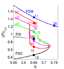
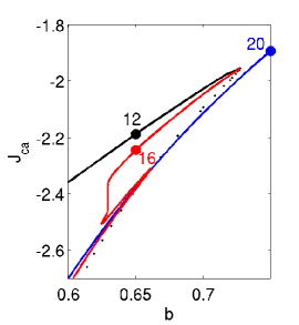
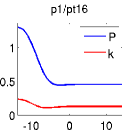
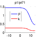
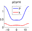
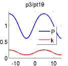
Figure 1: Example bifurcation diagrams and solution plots from running bdcmds.m. For $b<b_{\text{fold}}\approx 0.73$ there are three branches of FCSS, here called FSC (Flat State Clean, low $P$), FSI (Flat State Intermediate), and FSM (Flat State Muddy, high $P$). On FSC$\cup$FSI there are a number of bifurcations to patterned CSS branches. The BD in $J_{ca}$ in (b) shows that at, e.g., $b=0.65$ we have $J(\text{FSI})<J(\text{FMS})<J(\text{p1/pt71})<J(\text{p1/pt16})<J(\text{FSC})$, suggesting the FSC to be an optimal steady state. However, this does not exclude p1/pt16 or p1/pt71 to be optimal steady states, and moreover, there might be a path from the FSC to some other CSS with the SPP, dominating the FSC as a CSS. See [GU15] for further discussion.

%% stat. BD for sloc, main script-file. First set matlab paths: path(’../p2plib’,path);path(’../p2poclib’,path); %% ---- Scenario 1, FSC/FSI branch close all; p=[];lx=2*pi/0.44; ly=0.1; nx=50; ny=1; sw=1; p=slinit(p,lx,ly,nx,ny,sw); p=setfn(p,’f1’); screenlayout(p); p=cont(p,100); %% ---- FSM branch sw=2; p=slinit(p,lx,ly,nx,ny,sw); p=setfn(p,’f2’); p.nc.dsmax=0.2; p=cont(p,15); %% ---- bif from f1 (set bpt* and p* and repeat as necessary) p=swibra(’f1’,’bpt1’,’p1’,-0.05); p.nc.dsmax=0.3; p.nc.neigdet=50; p=cont(p,150); %% ---- plotting of BD, L2 and J_{ca}, and solution plots clf(3); pcmp=3; plotbraf(’f1’,’bpt1’,3,pcmp,’lab’,12,’cl’,’k’); % FSC (+ other branches) clf(3); pcmp=4; plotbraf(’f1’,’bpt1’,4,pcmp,’lab’,12,’cl’,’k’); % FSC (+other branches) plot1Df(’p1’,’pt16’,1,1,1,2); plot1Df(’p1’,’pt71’,2,1,1,2); % solution plots ... stancssvalf(’p1’,’pt16’); % extract values <P>, <k>, J_{c,a} from solution in p1/pt16;

Table 3: Selected commands from the script file bdcmds.m. See the source code for more details, and, e.g., bdcmds2D.m for the quite similar commands in 2D. Note that these files are in Matlab cell-modes, and the cells should be executed one by one. In the last command, p.fuha.con must be set.

Naturally, there are some modifications to the standard pde2path plotting commands, see, e.g., plot1D.m. These work as usual by overloading the respective pde2path functions by putting the adapted file in the current directory. See Fig. 1 for example results of running bdcmds.

2.1.2 Canonical paths

The goal is to calculate canonical paths from some starting state $v(0)$ to a CSS $\hat{u}_{1}$ with the SPP. For this we use one of the continuation algorithm iscnat or iscarc which in turn call mtom, based on TOM. Since we only wanted minimal modifications of TOM we found it convenient (though somewhat dangerous) to pass a number of parameters to the functions called by mtom via global variables. Thus, at the start of the canonical path scripts (here cpdemo.m) we define a number of global variables, see Table 4.

name	purpose
s0,s1	pde2path structs containing the boundary values at $t=0$ (s0) and at $t=T$ (s1)
Psi	the matrix $\Psi$ to encode the BC at $t=T$
u0, u1	vectors containing the current values of $u$ at the boundaries
par	the parameter values from s1 (only for convenience)
um1, um2	solutions at continuation steps $j-1$ and $j-2$ (to calculate secant predictors and used in extended system in iscarc)
sig	current (arclength) stepsize in iscarc

Table 4: Global variables for the computation of canonical paths, i.e., mainly for interfacing the driver scripts with the functions called by TOM.

The usage of p2poc to compute canonical paths is best understood by running and inspecting the demo file cpdemo.m.

(a) canonical path from p3/pt19 to FSC	(b) A fold in $\alpha$
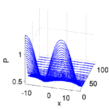
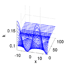
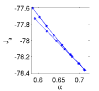
(c) The “upper” canonical path at $\alpha=0.6$	(d) diagnostics
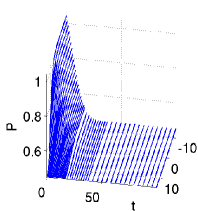
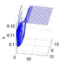
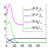
(e) The “lower” canonical path at $\alpha=0.6$	(f) diagnostics

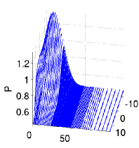
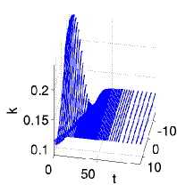
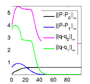
Figure 2: Example outputs from running slcpdemo.m

Some results of running cpdemo are shown in Fig. 2. (a) shows the “easy” case of a canonical path from p3/pt19 to FSC (up to line 11), while (b) to (f) illustrate the case of a fold in $\alpha$ when trying to get a canonical path from p1/pt71 to the FSC. (c)-(e) show the two canonical paths obtained from picking two canonical paths from the output of iscarc and a posteriori correcting to $\alpha=0.6$ (lines 24-26, only for the “upper” canonical path). Line 21 from slcpdemo prepares the calculation of Skiba paths, explained in §2.1.3. We now give a brief overview of the involved p2poclib functions, with the line-numbers refering to Table 6.

• (line 9)
  Input: alvin as the vector of desired $\alpha$ values, for instance alvin=[0.25 0.5 1]. sol,usec can be empty (typically on first call), but on subsequent calls should contain the last solution and the last secant (if opt.msw=1). fn is a structure containing the filenames for the start CSS and end CSS , and opt is an options structure containing TOM options and some more, see Table 5 and Remark 2.1.
  Output: alv as the $\alpha$ vector of successful solves; vv as the canonical path values $J_{a}$ of the successful solves; sol as the (last) canonical path; ydat contains the 2 last steps and the last secant (useful for repeated calls, and for using iscnat as startup for iscarc). Finally, if opt.retsw=1, then tlv,tv,uv contain data of all successful solves, namely: for the $j$-th step, j=1:length(alv), tlv(j), contains the meshsize (in $t$), tv(j,1:tlv(j)) the mesh, and uv(j,1:n,1:tlv(j) the solution. Thus, via sol.x=xv(j,1:tlv(j)); sol.y=squeeze(uv(j,
  1:n, 1:tlv(j))); the solution of the $j$-th step is recovered. This is useful for a posteriori inspecting some solution from the continuation (see line 24, and skiba.m in vegdemo). Note that uv can be large, and might give memory problems. If opt.retsw=0, then tlv,tv,uv are empty.

• (line 15)
  Input: as for iscnat (without alvin), but with esol containing the extended solution $(u_{\alpha},\alpha)$, and similar for the secant usec; as in iscnat, if opt.start=1, then esol,usec can be empty.
  Output: alv,val$\in{\mathbb{R}}^{1\times m}$ as the vectors of achieved $\alpha$ and $J_{a}(\alpha)$; usec,esol as the last secant/solution; tlv,tv,uv as in iscnat, but all in the sense of extended solutions, i.e. $(u_{\alpha},\alpha)$.

name	purpose	name	purpose
start	1 for startup, 0 else	M,lu,vsw	mass matrix, lu-switch and
retsw	1 to return full continuation data		(extra) verbosity for mtom
rhoi	index of $\rho$ in par	t1	truncation time $T$
nti	# of points in startup $t$–mesh	tv	current $t$–mesh
nsteps	number of steps for iscarc	sigmin,sigmax	min&max stepsize for iscarc

Table 5: Switches/controls in opt besides the TOM options. Note that iscarc only has a very elementary stepsize control via opt.sigmin,opt.sigmax.

Remark 2.1.

Concerning the original TOM options we remark that typically we run iscnat and iscarc with weak error requirements and what appears to be the fastest monitor and order options, i.e., opt.Monitor=3; opt.order=2;. Once continuation is successful (or also if it fails at some $\alpha$), we can always postprocess by calling mtom again with a higher order, stronger error requirements, and different monitor options, e.g., mesh–refinement based on condition rather than error alone. See the original TOM documentation.

1% driver script for Shallow Lake Optimal Control, first set paths and globals 2path(’../tom’,path); path(’../p2poclib’,path); 3close all; clear all; global s0 s1 u0 u1 Psi par xi ym1 ym2 sig; 4%% Preparations: put filenames into fn, set some bvp parameters 5sd0=’f1’; sp0=’pt12’; sd1=’p3’; sp1=’pt19’; flip=1; % p3->FSC 6fn=setfnflip(sd0,sp0,sd1,sp1,flip); opt=[]; opt=ocstanopt(opt); 7opt.rhoi=1; opt.t1=100; opt.start=1; opt.tv=[]; opt.nti=10; opt.retsw=0; 8%% the solve and continue call, and some plots 9sol=[]; alvin=[0.1 0.25 0.5 0.75 1]; v=[15,30]; 10[alv,vv,sol,ydat,tlv,xv,yv]=iscnat(alvin,sol,[],opt,fn); slsolplot(sol,v); 11%% ---- A fold in alpha, here iscarc needed. Prep. and initial iscarc call 12sd0=’f1’; sp0=’pt12’; sd1=’p1’; sp1=’pt71’; flip=1; fn=setfnflip(sd0,sp0,sd1,sp1,flip); 13esol=[]; ysec=[]; opt.nsteps=3; opt.alvin=[0.2 0.25]; sig=0.1; opt.nti=10; opt.tv=[]; 14opt.Stats_step=’on’; opt.start=1; opt.sigmax=1; opt.retsw=1; 15[alv,vv,ysec1,esol1,tlv,xv,yv]=iscarc(esol,ysec,opt,fn); opt.start=0; 16%% subsequent iccarc-calls (repeat this cell) 17opt.nsteps=20; ysec=ysec1; esol=esol1; % new input (for repeated calls) 18[alv1,vv1,ysec1,esol1,tlv1,xv1,yv1]=iscarc(esol,ysec,opt,fn); 19alv=[alv alv1]; vv=[vv vv1]; tlv=[tlv tlv1]; xv=[xv; xv1]; yv=[yv; yv1]; 20%% Postprocess sol from iscarc, first a simple plot of J over alpha 21alv0=alv; vv0=vv; xv0=xv; yv0=yv; tlv0=tlv; % save results for skibademo.m 22figure(6); clf; plot(alv(1,:),vv(1,:),’-*’);  xlabel(’\alpha’); ylabel(’J_{a}’); 23%% fix al from iscarc to some given value and compute CPs, first j=22, then j=34 24j=22; tl=tlv(j); n=s1.nu; sol.x=xv(j,1:tlv(j));sol.y=squeeze(yv(j,1:n,1:tlv(j))); 25al=0.6; u0=al*s0.u(1:n)+(1-al)*s1.u(1:n); u1=s1.u(1:s1.nu); 26opt.M=s1.mat.M; sol=mtom(@mrhs,@cbcf,sol,opt); v=[100,30]; slsolplot(sol,v);

Table 6: Selected commands from the script file cpdemo.m. See the source code for more details and, e.g., more fancy plotting.

The functions iscnat and iscarc are the two main user interface functions for the canonical path numerics. There are a number of additional functions for internal use, and some convenience functions, which we briefly review as follows:

• compute $\Psi$, the eigenvalues mu, the defect d, and a suggestion for $T$. Note that this becomes expensive with large $2nN$ (i.e., the total number of DoF).

• the ad–hoc modification of TOM, which allows for $M$ in (10a). Extra arguments $M$ and lu,vsw in opt. If opt.lu=0, then $\backslash$ is used for solving linear systems instead of an LU–decomposition, which becomes too slow when $nN\times m$ becomes too large. See the TOM documentation for all other arguments including opt, and note that the modifications in mtom can be identified by searching “HU” in mtom.m. Of course mtom (as any other function) can also be called directly (line 26), which for instance is useful to postprocess the output of some continuation by changing parameters by hand.

• the rhs and its Jacobian to be called within mtom. These are just wrappers which calculate $f$ and $J$ by calling the resp. functions in the pde2path–struct s1, which were already set up and used to calculate the CSS. s1 is passed as a global variable. Similar remarks apply to mrhse and fjace for the extended setting in iscarc.

• The boundary conditions (in time) for (10) and the associated Jacobians. Implemented by passing $u_{0},\hat{u}_{1},\Psi$ and similar globally. The *e (as in extended) versions are for iscarc.

• Calculate the objective value

  $$J(u)=\int_{0}^{T}{\rm e}^{-\rho t}J_{ca}(v(t,\cdot),k(t,\cdot))\,{\rm d}t$$ (23)

  of the solution $u$ in sol (with $J_{c}$ taken from s1.fuha.jcf), and similarly the normalized discounted value of a CSS contained in sol.y(:,end).

• generate the filename struct fn from sd0, sp0 (sd0/sp0.mat contains IC $u_{0}$) and sd1,sp1 (contains $\hat{u}$); if flip=1, then interchange *0 and *1.

• $x$–$t$ plots of canonical paths; plot component cmp of a canonical path sol to figure wnr, with view v and title tit. If cmp=0, then plot the control k, extracted from sol via p.fuha.con.

Thus, after having set up p as in §2.1.1 for the CSS, including $G$ and p.fuha.jcf, the user does not need to set up any additional functions to calculate canonical paths and their values. However, typically there are some functions which should be adapted to the given problem, e.g., for plotting, for instance

• (line 10) which calls:

• Plot some norms on a canonical path as functions of $t$ to figure(wnr). This is for instance useful to check the convergence behaviour of the canonical path as $t\rightarrow T$, cf. (d),(f) in Fig. 2.

2.1.3 A patterned Skiba point

In ODE OC applications, if there are several locally stable OSS, then often an important issue is to identify their domains of attractions. These are separated by so called theshhold or Skiba–points (if $N=1$) or Skiba–manifolds (if $N>1$), see [Ski78] and [GCF⁺08, Chapter 5]. Roughly speaking, these are initial states from which there are several optimal paths with the same value but leading to different CSS. In PDE applications, even under spatial discretization with moderate $nN$, Skiba manifolds should be expected to become very complicated objects. Thus, here we just give one example how to compute a patterned Skiba point between FSC and FSM.

In Line 17-19 of cpdemo.m we attempt to find a path from $P_{\text{PS}}$ given by p1/pt71 to $(P,q)_{\text{FSC}}$ given by FSC/pt12; this fails due to the fold in $\alpha$. However, for given $\alpha$ we can also try to find a path from the initial state $P_{\alpha}(0):=\alpha P_{\text{PS}}+(1-\alpha)P_{\text{FSC}}$ to the FSM, and compare to the path to the FSC. For this, in line 21 of cpdemo.m, we stored the $\alpha$ and $J_{ca}$ values into alv0, vv0, and also the path data into tlv0,tv0 uv0. See skibademo.m in Table 7 (in particular line 11 and the following) how to put the values uv0(j,:,1) into s0 and subsequently find the paths to the FSM, and Fig. 3 for illustration.

1% Skiba example, continues cpdemo.m 2% find paths from the yv0 initial states from cpdemo.m to FSM 3js=10; je=30; jl=js-je+1; % alpha-range; now set the target and Psi to FSM: 4s1=loadp(’f2’,’pt11’); u1=s1.u(1:s1.nu); [Psi,muv,d,t1]=getPsi(s1); 5a0l=length(alv0); tva=zeros(jl,opt.Nmax+1); % some prep. and fields to hold paths 6uva=zeros(jl,n+1,opt.Nmax+1); alva=[]; vva=[]; tavl=[]; sol=[]; 7alvin=[0.1 0.25 0.5 0.75 1]; % we run from uv0(j,:) to FSM with iscnat 8tv=linspace(0,opt.t1,opt.nti); se=2; opt.tv=tv.^se./opt.t1^(se-1); doplot=1; 9opt.msw=0; opt.Stats_step=’off’; v=[50,8]; % switch off stats 10for j=js:je; 11   fprintf(’j=%i, al=%g\n’, j, alv0(j)); s0.u(1:n)=uv0(j,1:n,1)’; 12   [alv,vv,sol,udat]=iscnat(alvin,[],[],opt,fn); 13   if alv(end)==1; Jd=vv0(j)-vv(end); fprintf(’J1-J2=%g\n’,Jd); % contin. successful 14      alva=[alva alv0(j)]; vva=[vva vv(end)]; tl=length(sol.x); % put vals in vector 15      tavl=[tavl tl]; tva(j,1:tl)=sol.x; uva(j,1:n,1:tl)=sol.y; 16      if abs(Jd)<0.05; doplot=asknu(’plot path?’,doplot); % Skiba point(s) found 17        if doplot==1; sol0=[]; alp=alv0(j); % plot the paths to FSC and FSM 18          sol0.x=tv0(j,1:tlv0(j));sol0.y=squeeze(uv0(j,1:n,1:tlv0(j))); 19          psol3Dm(s1,sol0,sol,1,1,[]); view(v); zlabel(’P’); pause 20        end 21      end 22   end 23end 24%% plot value diagram 25figure(6); plot(alv0(js:jep),vv0(js:jep),’-*b’);hold on;plot(alva,vva,’-*r’); 26xlabel(’\alpha’,’FontSize’,s1.plot.fs); ylabel(’J_{a}’,’FontSize’,s1.plot.fs);

Table 7: The script file skibademo.m. See text for comments.

(a) A Skiba point at $\alpha=0.454$	(b) Paths to FSC (blue) and FSM (red)

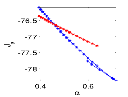
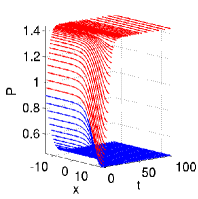
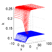
Figure 3: Example outputs from skibademo.m

2.1.4 Further comments

To keep the demos simple, here we do not include versions of iscnat and iscarc that use the truncation time $T$ as an additional free parameter [GU15, Fig.5]. However, the files bdcmds.m and cpdemo.m also contain some of the commands used to study Scenario 2, see [GU15, §2.3] for the results, and the directory slocdemo contains the script files bdcmds2D.m and cpdemo2D.m, used to compute CSS and canonical paths for (22) over the 2D domain $\Omega=(-L,L)\times(-\frac{L}{2},\frac{L}{2})$ (based on exactly the same init file slinit.m), some auxiliary plotting functions plotsolf.m and plotsolfu.m, and the function sol2mov.m used to generate movies of canonical paths. See, e.g., [GU15, Fig. 7,8] for some results, while some movies can be downloaded at the pde2path homepage.

2.2 The vegOC model

Our second example, from [Uec15], concerns the optimal control of a reaction diffusion system used to model grazing in a semi arid system for biomass (vegetation) $v$ and soil water $w$, following [BX10]. Here, semi arid means that there is enough water to support some vegetation, but not enough water for a dense homogeneous vegetation. This is an important problem as it is estimated that semi arid areas cover about 40% of the world’s land area and support about two billion people, often by grazing livestock, www.allcountries.org/maps/world_climate_maps.html. In semi arid areas, often overgrazing is a serious threat as it may lead to irreversible desertification, see, e.g., [SBB⁺09], and the references therein.

Denoting the harvesting (grazing) effort as the control by $E$, we consider

$$V(v_{0},w_{0}) =\max_{E(\cdot,\cdot)}J(v_{0},w_{0},E),$$ (24a)

$${\partial}_{t}v =d_{1}\Delta v+[gwp^{\eta}-d(1+\delta v)]v-H,$$ (24b)

$${\partial}_{t}w =d_{2}\Delta w+R(\beta+\xi v)-(r_{u}v+r_{w})w,$$ (24c)

with harvest $$H=v^{\alpha}E^{1-\alpha} J_{c}=J_{c}(v,E)=pH-cE p c v E 0<\alpha<1 (g,\eta,d,\delta,\beta,\xi,r_{u},r_{w},d_{1,2}) \rho=0.03,p=1.1,\alpha=0.3,c=1 R$$, and current value objective function , which thus depends on the price , the costs for harvesting/grazing, and , in a classical Cobb–Douglas form with elasticity parameter . For the modeling, and the meaning and values of the parameters we refer to [BX10, Uec15] and the references therein (see also Table 8, line 9 for the parameter values), and here only remark that are the economic parameters, and we take the rainfall as the main bifurcation parameter. Furthermore, we have the BC and IC

$${\partial}_{\nu}v={\partial}_{\nu}w=0\text{ on }{\partial}\Omega,\quad(v,w)|_{t=0}=(v_{0},w_{0}).$$ (24d)

Denoting the co-states by $(\lambda,\mu)$ we have the local current value Hamiltonian

$${\cal H}(v,w,\lambda,\mu,E)=J_{c}(v,E) +\lambda\bigl{[}d_{1}\Delta v+(gwp^{\eta}-d(1+\delta v))v-H\bigr{]}$$

$$+\mu\bigl{[}d_{2}\Delta w+R(\beta+\xi v)-(r_{u}v+r_{w})w\bigr{]},$$ (25)

and obtain the canonical system

$${\partial}_{t}v ={\cal H}_{\lambda}=d_{1}\Delta v+[gwp^{\eta}-d(1+\delta v)]v-H,$$ (26a)

$${\partial}_{t}w ={\cal H}_{\mu}=d_{2}\Delta w+R(\beta+\xi v)-(r_{u}v+r_{w})w,$$ (26b)

$${\partial}_{t}\lambda =\rho\lambda-{\cal H}_{v}=\rho\lambda-p\alpha v^{\alpha-1}E^{1-\alpha}-\lambda\bigl{[}g(\eta+1)wv^{\eta}-2d\delta v-d-\alpha v^{\alpha-1}E^{1-\alpha}]$$ (26c)

$$\qquad\qquad\qquad-\mu(R\xi-r_{u})w-d_{1}\Delta\lambda,$$

$${\partial}_{t}\mu =\rho\mu-{\cal H}_{w}=\rho\mu-\lambda gv^{\eta+1}+\mu(r_{u}v+r_{w})-d_{2}\Delta\mu,$$ (26d)

where $$E {\partial}_{E}{\cal H}=0$$ is obtained from solving , giving

$$E=\left(\frac{c}{(p-\lambda)(1-\alpha)}\right)^{-1/\alpha}v.$$ (26e)

With the notation $$u=(v,w,\lambda,\mu)$$, the IC, the BC, and the transversality condition are

$$(v,w)|_{t=0}=(v_{0},w_{0}),\quad{\partial}_{\nu}u=0\text{ on }{\partial}\Omega,\quad\lim_{t\to\infty}{\rm e}^{-\rho t}u(t)=0.$$ (26f)

To study (26), we write it as ${\partial}_{t}u=-G(u)$ and basically need to set up $G$ and the BC. This follows the general pde2path settings with the OC related modifications already explained in §2.1, and thus we only give the following remarks, first concerning veginit.m, see Table 8.

• we only set up p.fuha.sG since in this demo we use p.sw.jac=0 (numerical Jacobians), and hence do not need to set p.fuha.sGjac.

• set the Neumann BC and diffusion tensor for the 4 component system (see gnbc.m and isoc.m for documentation)

• set the desired $R$ values for output of CSS to disk, the parameter values, and the main bifurcation parameter. Of course, one could also hard-code all parameters except $R$, but we generally recommend to treat parameters as parameters since this is needed if later a continuation in some other parameter is desired, and since it usually makes the code more readable.

1function p=veginit(p,lx,ly,nx,ny,sw,rho) % init-routine for vegOC 2p=stanparam(p); p.nc.neq=4; p.fuha.sG=@vegsG; p.fuha.jcf=@vegjcf; p.fuha.outfu=@ocbra; 3p.mesh.geo=rec(lx,ly); p=stanmesh(p,nx,ny); p.sol.xi=0.005/p.np; % generate mesh 4q=zeros(p.nc.neq); g=zeros(p.nc.neq,1); % setting up Neumann BC for 4 components 5bc=gnbc(p.nc.neq,4,q,g); p.fuha.bc=@(p,u) bc; p.fuha.bcjac=@(p,u) bc; 6p.d1=0.05; p.d2=10; p.eqn.a=0; p.eqn.b=0; % setting up K for 4 components 7c=diag([p.d1, p.d2, -p.d1, -p.d2]); p.eqn.c=isoc(c,4,1); 8p.usrlam=[4 10 20 26 28]; % desired R values for output of CSS 9par=[rho 1e-3 0.5 0.03 0.005 0.9 1e-3 34 0.01 0.1 1 1.1 0.3]; % par-values 10p.nc.ilam=8;  % choose the active par, here Rainfall R 11% now continue with setting a few more param and the initial guess ... see veginit.m

Table 8: Selected commands from the init-routine veginit.m. See the source code for more details.

Table 9 shows the complete codes for setting up $G$ and the current value $J_{c}$. Both use the auxiliary function efu, which is also used in, e.g., valf.m to tabulate characteristical values of CSS.

1function r=vegsG(p,u) % rhs for vegOC problem 2par=u(p.nu+1:end); rho=par(1); g=par(2); eta=par(3); % extract param 3d=par(4); del=par(5); beta=par(6); xi=par(7); rp=par(8); up=par(9); rw=par(10); 4cp=par(11); pp=par(12); al=par(13); [e,h,J]=efu(p,u);  % calculate H 5v=u(1:p.np); w=u(p.np+1:2*p.np); % extract soln-components, states 6l1=u(2*p.np+1:3*p.np); l2=u(3*p.np+1:4*p.np); % co-states 7f1=(g*w.*v.^eta-d*(1+del*v)).*v-h; f2=rp*(beta+xi*v)-(up*v+rw).*w; % f1,f2 8f3=rho*l1-pp*al*h./v-l1.*(g*(eta+1)*w.*v.^eta-2*d*del*v-d-al*h./v)-l2.*(rp*xi-up*w); 9f4=rho*l2-l1.*(g*v.^(eta+1))-l2.*(-up*v-rw); f=[f1;f2;f3;f4]; 10r=p.mat.K*u(1:p.nu)-p.mat.M*f; % the residual
1function jc=vegjcf(p,u); [e,h,jc]=efu(p,u); % J_c for vegOC, here just an interface
1function [e,h,J]=efu(p,varargin) % extract [e,h,J] from p or u 2if nargin>1 u=varargin{1}; else u=p.u; end 3par=p.u(p.nu+1:end); cp=par(11); pp=par(12); al=par(13); 4v=u(1:p.np); l1=u(2*p.np+1:3*p.np); 5gas=((pp-l1)*(1-al)./cp).^(1/al); e=gas.*v; h=v.^al.*e.^(1-al); 6J=pp*v.^al.*e.^(1-al)-cp*e;

Table 9: Implementation of the rhs $G$ and $J_{c}$ for (26), and the aux function efu.

Figure 4 shows a basic bifurcation diagram of CSS in 1D with $\Omega=(-L,L)$, $L=5$, from the script file vegbd1d.m, which follows the same principles as the one for the SLOC demo. The blue branch in (a) represents the primary bifurcation of PCSS, which for certain $R$ have the SPP, and, moreover, are POSS. See also [Uec15] for more plots, including a comparison with the uncontrolled case of so called “private optimization”, and 2D results for $\Omega=(-L,L)\times(-\sqrt{3}L/2,\sqrt{3}L/2)$ yielding various POSS, including hexagonal patterns.

(a)                                                                   (b)                                  (c)
 

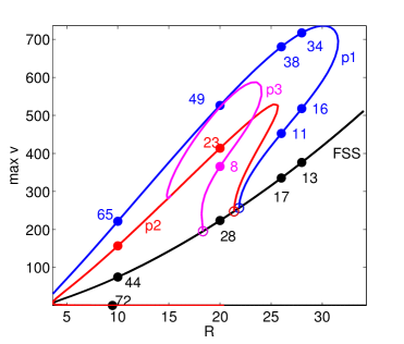
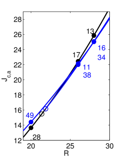
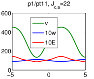
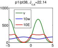
Figure 4: Outputs of bd1ddemo.m. (a),(b) bifurcation diagrams of CSS in 1D; (c) example solutions.

The script files vegcpdemo.m for canonical paths, and vegskiba.m for a Skiba point between the flat optimal steady state FSS/pt13 and the POSS p1/pt34, again follow the same principles as in the the SLOC demo. See Figures 5, and 6 for example outputs, and [Uec15] for a detailed discussion. In a nutshell, we find that:

• For large $R$ the FCSS is the unique CSS of (26), and is optimal, hence a globally stable FOSS (Flat Optimal Steady State).

• For smaller $R$ there are branches of (locally stable) POSS (Patterned Optimal Steady States), which moreover dominate all other CSS.

• For the uncontrolled problem, Flat Steady States (FSS) only exist for much larger $R$ than the FCSS under control.

• At equal $R$, the profit $J$ (or equivalently the discounted value $J_{c}/\rho$) of the uncontrolled FSS is much lower than the value of the FCSS under control.

(a) $R=26$, the canonical path from the lower PCSS(p1/pt11) to the FCSS (FSS/pt17)

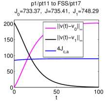
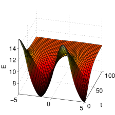
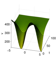
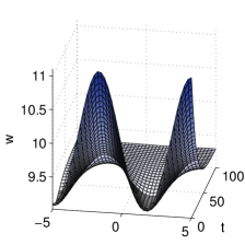
(b) $R=26$, the canonical path from the FCSS to the upper PCSS (p1/pt38)

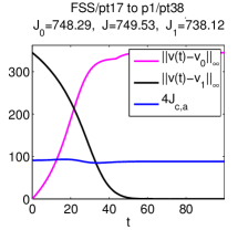
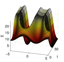
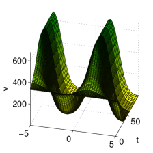
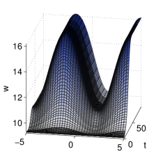
Figure 5: Example output of vegcpdemo.m: Two canonical paths. The leftmost panels indicate the convergence behaviour, the current value profits, and obtained objective values. The middle and right panels show the strategy $E$ and the corresponding behaviour of $(v,w)$. See [Uec15] for comments and more details.

(a) A Skiba point at $\alpha\approx 0.9$	(b) Paths of (almost) equal values to the FCSS and the upper PCSS.

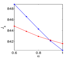
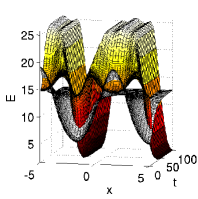
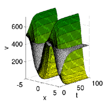
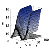
Figure 6: $R=28$, example outputs from skibademo.m. In (a), the blue line gives $J$ for the canonical path $t\mapsto u(t)$ from $(v,w)_{\alpha}(0):=\alpha(v,w)_{\text{PS}}+(1-\alpha)(v,w)_{\text{FSS}}$, where FSS denotes FSS/pt13, and PS denotes p1/pt16. The red line gives $J$ for the CP $t\mapsto\tilde{u}(t)$ from $P_{\alpha}(0)$ to the upper PCSS p1/pt34. Similarly, the white surfaces in (b) are for $u$ and the colored ones for $\tilde{u}$. $R=28$.

3 Summary and outlook

With p2poc we provide a toolbox to study OC problems of class (1) in a simple and convenient way, in 1D and 2D. The class (1) is quite general, and with the pde2path machinery we have a rather powerful tool to study the bifurcations of CSS. The computation of canonical paths is comparatively more involved. Essentially, our step (b) implements for the class (1) (parts of) the methods explained for ODE problems in [GCF⁺08, Chapter 7], and implemented in OCMat orcos.tuwien.ac.at/research/ocmat_software/, see also [Gra15] for an extension of OCMat to 1D systems of class (1). In a somewhat more general sense, step (b) is a special case (for PDEs) of the “connecting orbit method”. See [DCF⁺97, BPS01] and the references therein for earlier work on connecting orbits in ODE problems, including connecting orbits to periodic solutions, which for ODE OC problems may also be important as long-run optimal solutions, again cf. [GCF⁺08]. Our setup for (b) is reasonably fast for up to 4000 degrees of freedom of $u$ at fixed time, e.g., 1000 spatial discretization points and 4 components, and up to 200 temporal discretization points, i.e., up to these values a continuation step in the calculation of a canonical path takes up to a few minutes on a desktop computer.

Of course, there is a rather large number of issues we do not address (yet). Besides periodic long-run optimal solutions, one of these are state or control inequality constraints that frequently occur in OC problems. For instance, in the SLOC model we need non-negativity of $P$ and $k$, and similarly of $v,w$ and $E$ in the vegOC model. In our examples we simply checked these a posteriori and found them to be always fulfilled, i.e., inactive. If such constraints become active the problem becomes much more complicated. Some extensions in this direction will be added as required by examples.

Clearly, it is tempting to recombine steps (a) and (b) again, at least for specific purposes. One example would be the continuation of canonical paths in a parameter $\eta$. Naively, this could be done “by hand” by using a canonical path $u(\cdot,\eta)$ between $v_{0}$ (or $v_{0}(\eta)$) and $\hat{u}(\eta)$ as an initial guess for a canonical path $u(\cdot,\eta+\delta)$ between $v_{0}$ (or $v_{0}(\eta+\delta)$) and $\hat{u}(\eta+\delta)$, at the parameter value $\eta+\delta$. This, however, does not directly allow to check for bifurcations of canonical paths, and, perhaps more importantly, requires the recalculation of $\Psi$ at each new $\hat{u}(\eta)$. See [BPS01, Pam01] for the “boundary corrector method” as an approach to avoid the latter, and, moreover, for continuation methods in the full t-BVP that for instance also allow the computation of Skiba-curves (cf.§2.1.3) in 0D, cf. also [GCF⁺08, §7.7–§7.8].

As currently p2pOC is based on pde2path, it works most efficiently for spatial 2D problems, while 1D problems are treated as very narrow quasi 1D strips. Presently, pde2path is extended to efficiently treat also 1D and 3D problems, based on the package OOPDE www.mathe.tu-freiberg.de/nmo/mitarbeiter/uwe-pruefert/software. Thus, p2pOC will soon provide a genuine 1D setting as well.

References

- [AAC11] S. Aniţa, V. Arnăutu, and V. Capasso. An introduction to optimal control problems in life sciences and economics. Birkhäuser/Springer, New York, 2011.
- [ACKLT13] S. Aniţa, V. Capasso, H. Kunze, and D. La Torre. Optimal control and long-run dynamics for a spatial economic growth model with physical capital accumulation and pollution diffusion. Appl. Math. Lett., 26(8):908–912, 2013.
- [ADS14] N. Apreutesei, G. Dimitriu, and R. Strugariu. An optimal control problem for a two-prey and one-predator model with diffusion. Comput. Math. Appl., 67(12):2127–2143, 2014.
- [BPS01] W.J. Beyn, Th. Pampel, and W. Semmler. Dynamic optimization and Skiba sets in economic examples. Optimal Control Applications and Methods, 22(5–6):251–280, 2001.
- [BX08] W.A. Brock and A. Xepapadeas. Diffusion-induced instability and pattern formation in infinite horizon recursive optimal control. Journal of Economic Dynamics and Control, 32(9):2745–2787, 2008.
- [BX10] W. Brock and A. Xepapadeas. Pattern formation, spatial externalities and regulation in coupled economic–ecological systems. Journal of Environmental Economics and Management, 59(2):149–164, 2010.
- [CPB12] C. Camacho and A. Pérez-Barahona. Land use dynamics and the environment. Documents de travail du Centre d’Economie de la Sorbonne, 2012.
- [DCF+97] E. Doedel, A. R. Champneys, Th. F. Fairgrieve, Y. A. Kuznetsov, Bj. Sandstede, and X. Wang. AUTO: Continuation and bifurcation software for ordinary differential equations (with HomCont). http://cmvl.cs.concordia.ca/auto/, 1997.
- [DRUW14] T. Dohnal, J. Rademacher, H. Uecker, and D. Wetzel. pde2path 2.0. In H. Ecker, A. Steindl, and S. Jakubek, editors, ENOC 2014 - Proceedings of 8th European Nonlinear Dynamics Conference, ISBN: 978-3-200-03433-4, 2014.
- [GCF+08] D. Grass, J.P. Caulkins, G. Feichtinger, G. Tragler, and D.A. Behrens. Optimal Control of Nonlinear Processes: With Applications in Drugs, Corruption, and Terror. Springer Verlag, 2008.
- [Gra15] D. Grass. From 0D to 1D spatial models using OCMat. Technical report, ORCOS, 2015.
- [GU15] D. Grass and H. Uecker. Optimal management and spatial patterns in a distributed shallow lake model. Preprint, 2015.
- [KW10] T. Kiseleva and F.O.O. Wagener. Bifurcations of optimal vector fields in the shallow lake system. Journal of Economic Dynamics and Control, 34(5):825–843, 2010.
- [MS02] F. Mazzia and I. Sgura. Numerical approximation of nonlinear BVPs by means of BVMs. Applied Numerical Mathematics, 42(1–3):337–352, 2002. Numerical Solution of Differential and Differential-Algebraic Equations, 4-9 September 2000, Halle, Germany.
- [MST09] F. Mazzia, A. Sestini, and D. Trigiante. The continuous extension of the B-spline linear multistep methods for BVPs on non-uniform meshes. Applied Numerical Mathematics, 59(3–4):723–738, 2009.
- [MT04] F. Mazzia and D. Trigiante. A hybrid mesh selection strategy based on conditioning for boundary value ODE problems. Numerical Algorithms, 36(2):169–187, 2004.
- [NPS11] I. Neitzel, U. Prüfert, and Th. Slawig. A smooth regularization of the projection formula for constrained parabolic optimal control problems. Numer. Funct. Anal. Optim., 32(12):1283–1315, 2011.
- [Pam01] Th. Pampel. Numerical approximation of connecting orbits with asymptotic rate. Numerische Mathematik, 90(2):309–348, 2001.
- [RZ99a] J. P. Raymond and H. Zidani. Hamiltonian Pontryagin’s principles for control problems governed by semilinear parabolic equations. Appl. Math. Optim., 39(2):143–177, 1999.
- [RZ99b] J. P. Raymond and H. Zidani. Pontryagin’s principle for time-optimal problems. J. Optim. Theory Appl., 101(2):375–402, 1999.
- [SBB+09] M. Scheffer, J. Bascompte, W. A. Brock, V. Brovkin, St. R. Carpenter, V. Dakos, H. Held, E. H. van Nes, M. Rietkerk, and G. Sugihara. Early-warning signals for critical transitions. Nature, 461:53–59, 2009.
- [Ski78] A. K. Skiba. Optimal growth with a convex-concave production function. Econometrica, 46(3):527–539, 1978.
- [Trö10] Fredi Tröltzsch. Optimal control of partial differential equations, volume 112 of Graduate Studies in Mathematics. American Mathematical Society, Providence, RI, 2010.
- [Uec15] H. Uecker. Optimal control and spatial patterns in a semi arid grazing system. Preprint, 2015.
- [UWR14] H. Uecker, D. Wetzel, and J. Rademacher. pde2path – a Matlab package for continuation and bifurcation in 2D elliptic systems. NMTMA, 7:58–106, 2014. see also www.staff.uni-oldenburg.de/hannes.uecker/pde2path.