Convergence of Alternating Least Squares Optimisation for Rank-One Approximation to High Order Tensors

Abstract

The approximation of tensors has important applications in various disciplines, but it remains an extremely challenging task. It is well known that tensors of higher order can fail to have best low-rank approximations, but with an important exception that best rank-one approximations always exists. The most popular approach to low-rank approximation is the alternating least squares (ALS) method. The convergence of the alternating least squares algorithm for the rank-one approximation problem is analysed in this paper. In our analysis we are focusing on the global convergence and the rate of convergence of the ALS algorithm. It is shown that the ALS method can converge sublinearly, Q-linearly, and even Q-superlinearly. Our theoretical results are illustrated on explicit examples.

Keywords: tensor format, tensor representation, alternating least squares optimisation, orthogonal projection method.

MSC: 15A69, 49M20, 65K05, 68W25, 90C26.

1 Introduction

We consider a minimisation problem on the tensor space $\mathcal{V}=\bigotimes_{\mu=1}^{d}\mathds{R}^{n_{\mu}}$ equipped with the Euclidean inner product $\left\langle\cdot,\cdot\right\rangle$. The objective function $f:\mathcal{V}\rightarrow\mathds{R}$ of the optimisation task is quadratic

$$f(v):=\frac{1}{\|b\|^{2}}\left[\frac{1}{2}\left\langle v,v\right\rangle-\left\langle b,v\right\rangle\right]\geq-\frac{1}{2},$$ (1)

where $b\in\mathcal{V}$. In our analysis, a tensor $u\in\mathcal{V}$ is represented as a rank-one tensor. The representation of rank-one tensors is described by the following multilinear map $U$:

$$U:P:=\mathop{\mathchoice{\raise-2.20001pt\hbox{\huge$\times$}}{\raise-0.50003pt\hbox{\Large$\times$}}{\hbox{\large$\times$}}{\times}}_{\mu=1}^{d}\mathds{R}^{n_{\mu}} \rightarrow \mathcal{V}$$

$$(p_{1},\dots,p_{d}) \mapsto U(p_{1},\dots,p_{d}):=\bigotimes_{\mu=1}^{d}p_{\mu}.$$

We call a $d$-tuple of vectors $(p_{1},\dots,p_{d})\in P$ a representation system of $u$ if $u=U(p_{1},\dots,p_{d})$. The tensor $b$ is approximated with respect to rank-one tensors, i.e. we are looking for a representation system $(p^{*}_{1},\dots,p^{*}_{d})\in P$ such that for

$$F := f\circ U:P\rightarrow\mathcal{V}\rightarrow\mathds{R}$$ (2)

$$F(p_{1},\dots,p_{d}) = \frac{1}{\|b\|^{2}}\left[\frac{1}{2}\left\langle U(p_{1},\dots,p_{d}),U(p_{1},\dots,p_{d})\right\rangle-\left\langle b,U(p_{1},\dots,p_{d})\right\rangle\right]$$

we have

$$F(p^{*}_{1},\dots,p^{*}_{d})=\min_{(p_{1},\dots,p_{d})\in P}F(p_{1},\dots,p_{d}).$$ (3)

The range set $U(P)$ is a closed in $\mathcal{V}$, see [6]. Therefore, the approximation problem is well defined. The set of best rank-one approximations of the tensor $b$ is denoted by

$$\mathcal{M}_{b}:=\left\{v\in U(P)\,:\,v\mbox{ is a best rank-one approximation of }b\right\}.$$ (4)

The alternating least squares (ALS) algorithm [2, 3, 4, 7, 8, 11, 12] is recursively defined. Suppose that the $k$-th iterate $\underline{p}^{k}=(p_{1}^{k},\dots,p_{d}^{k})$ and the first $\mu-1$ components $p_{1}^{k+1},\dots,p_{\mu-1}^{k+1}$ of the $(k+1)$-th iterate $\underline{p}^{k+1}$ have been determined. The basic step of the ALS algorithm is to compute the minimum norm solution

$$p_{\mu}^{k+1}:=\mbox{\rm argmin}_{q_{\mu}\in\mathds{R}^{n_{\mu}}}F(p_{1}^{k+1},\dots,p_{\mu-1}^{k+1},q_{\mu},p_{\mu+1}^{k},\dots,p_{d}^{k}).$$

Thus, in order to obtain $\underline{p}^{k+1}$ from $\underline{p}^{k}$, we have to solve successively $L$ ordinary least squares problems.

The ALS algorithm is a nonlinear Gauss-Seidel method. The locale convergence of the nonlinear Gauss-Seidel method to a stationary point $\underline{p}^{*}\in P$ follows from the convergence of the linear Gauss-Seidel method applied to the Hessian $F^{\prime\prime}(\underline{p}^{*})$ at the limit point $\underline{p}^{*}$. If the linear Gauss-Seidel method converges R-linear then there exists a neighbourhood $B(\underline{p}^{*})$ of $\underline{p}^{*}$ such that for every initial guess $\underline{p}^{0}\in B(\underline{p}^{*})$ the nonlinear Gauss-Seidel method converges R-linear with the same rate as the linear Gauss-Seidel method. We refer the reader to Ortega and Rheinboldt for a description of nonlinear Gauss-Seidel method [10, Section 7.4] and convergence analysis [10, Thm. 10.3.5, Thm. 10.3.4, and Thm. 10.1.3]. A representation system of a represented tensor is not unique, since the map $U$ is multilinear. Consequently, the matrix $F^{\prime\prime}(\underline{p}^{*})$ is not positive definite. Therefore, convergence of the linear Gauss-Seidel method is in general not ensured. However, the convergence of the ALS method is discussed in [9, 13, 15, 16]. Recently, the convergence of the ALS method was analysed by means of Lojasiewicz gradient inequality, please see [14] for more details. The current analysis is not based on the mathematical techniques developed for the nonlinear Gauss-Seidel method neither on the theory of Lojasiewicz inequalities, but on the multilinearity of the map $U$.

Notation 1.1 ($\mathds{N}_{n}$).

The set $\mathds{N}_{n}$ of natural numbers smaller than $n\in\mathds{N}$ is denoted by

$$\mathds{N}_{n}:=\{j\in\mathds{N}:1\leq j\leq n\}.$$

The precise analysis of the ALS method is a quite challenging task. Some of the difficulties of the theoretical understanding are explained in the following examples.

Example 1.2.

The approximation of $b\in\mathcal{V}$ by a tensor of rank one is considered, where

$$b = \sum_{j=1}^{r}\underbrace{\lambda_{j}\bigotimes_{\mu=1}^{d}b_{j\mu}}_{b_{j}:=},\quad\lambda_{1}\geq\dots\geq\lambda_{r}>0,\,\|b_{j\mu}\|=1,$$ (5)

$$B_{\mu} := \left(b_{j\mu}:1\leq j\leq r\right)\in\mathds{R}^{m_{\mu}\times r}\quad(1\leq\mu\leq d),$$

and $B_{\mu}^{T}B_{\mu}=\mbox{\bf Id}$, see the example in [9, Section 4.3.5]. Let us further assume that $v_{k}=p_{1}^{k}\otimes p_{2}^{k}\otimes\dots\otimes p_{d}^{k}$ is already determined. Corollary 2.4 leads to the recursion

$$p_{1}^{k+1}=\underbrace{\left[\frac{1}{\|v_{k}\|^{2}}B_{1}\mbox{\rm diag$\,$}\left(\lambda_{j}^{2}\prod_{\mu=2}^{d-1}\frac{\left\langle b_{j\mu},p_{\mu}^{k}\right\rangle}{\|p_{\mu}^{k}\|^{2}}^{2}\right)_{j=1,\dots,r}B_{1}^{T}\right]}_{G_{1}(p_{1}^{k},\dots,p_{d}^{k}):=}p_{1}^{k}\quad(k\geq 2).$$ (6)

The linear map $G_{1}(p_{1}^{k},\dots,p_{d}^{k})\in\mathds{R}^{m_{1}\times m_{1}}$ describes the first micro step $p_{1}^{k}\otimes p_{2}^{k}\otimes\dots\otimes p_{d}^{k}\quad\mapsto p_{1}^{k+1}\otimes p_{2}^{k}\otimes\dots\otimes p_{d}^{k}$ in the ALS algorithm. The iteration matrix $G_{1}(p_{1}^{k},\dots,p_{d}^{k})$ is independent under rescaling of the representation system, i.e. $G_{1}(\alpha_{1}p_{1},\dots,\alpha_{d}p_{d})=G_{1}(p_{1},\dots,p_{d})$ for $1=\prod_{\mu=1}^{d}\alpha_{\mu}$. Further, we can illustrate the difficulties of the ALS iteration in higher dimensions. For $d=2$, the ALS method is given by the two power iterations

$$p_{1}^{k+1} = \left[\frac{1}{\|p_{1}^{k}\|^{2}\|p_{2}^{k}\|^{2}}B_{1}\mbox{\rm diag$\,$}\left(\lambda_{j}^{2}\right)_{j=1,\dots,r}B_{1}^{T}\right]p_{1}^{k},$$

$$p_{2}^{k+1} = \left[\frac{1}{\|p_{1}^{k+1}\|^{2}\|p_{2}^{k}\|^{2}}B_{2}\mbox{\rm diag$\,$}\left(\lambda_{j}^{2}\right)_{j=1,\dots,r}B_{2}^{T}\right]p_{2}^{k}.$$

Clearly, if the global minimum $b_{1}$ is isolated, i.e. $\lambda_{1}>\lambda_{2}$, then the ALS method converges to $b_{1}$ provided that $\left\langle v_{0},b_{1}\right\rangle\neq 0$, where $v_{0}=p_{1}^{0}\otimes p_{2}^{0}\in\mathcal{V}$ is the initial guess. Further, we have linear convergence

$$\left|\tan\angle[b_{1\,\mu},p_{\mu}^{k+1}]\right|\leq\left(\frac{\lambda_{2}}{\lambda_{1}}\right)^{2}\,\left|\tan\angle[b_{1\,\mu},p_{\mu}^{k}]\right|\quad(1\leq\mu\leq 2).$$

Note that in this example the angle $\angle[b_{1\,\mu},p_{\mu}^{k}]$ is a more natural measure of the error than the usual distance $\|b_{1\,\mu}-p_{\mu}^{k}\|$. For $d\geq 3$, the factor $\prod_{\mu=2}^{d-1}\left\langle b_{j\mu},p_{\mu}^{k}\right\rangle^{2}/\|p_{\mu}^{k}\|^{2}$ from Eq. (6) describes the behaviour of the ALS iteration. Let $1\leq j^{*}\leq r$. We say that a term $b_{j^{*}}$ from Eq. (5) dominates at $v_{k}=p_{1}^{k}\otimes\dots\otimes p_{d}^{k}$ if

$$\sqrt[d-2]{\lambda_{j^{*}}^{2}}\left\langle b_{j^{*}\mu},p_{\mu}^{k}\right\rangle^{2}>\sqrt[d-2]{\lambda_{j}^{2}}\left\langle b_{j\mu},p_{\mu}^{k}\right\rangle^{2}$$ (7)

for all $j\in N_{j^{*}}:=\left\{j\in\mathds{N}\,:\,1\leq j\leq r\mbox{ and }j\neq j^{*}\right\}$ and all $\mu\in\mathds{N}_{d}$. If $b_{j^{*}}$ dominates at $v_{k}$, then the recursion formula (6) leads to

$$\left|\tan\angle[b_{j^{*}\,1},p_{1}^{k+1}]\right|\leq\underbrace{\frac{\max_{j\in N_{j^{*}}}\left(\lambda_{j}\prod_{\mu=2}^{d-1}\left\langle b_{j\mu},p_{\mu}^{k}\right\rangle\right)^{2}}{\left(\lambda_{j^{*}}\prod_{\mu=2}^{d-1}\left\langle b_{j^{*}\mu},p_{\mu}^{k}\right\rangle\right)^{2}}}_{<1}\,\left|\tan\angle[b_{j^{*}\,1},p_{1}^{k}]\right|,$$ (8)

i.e. the first component of the representation system $p_{1}^{k+1}$ is turned towards the direction of $b_{j^{*}\,1}$. Note that for $r=2$ the bound for the convergence rate is sharp, i.e.

$$\left|\tan\angle[b_{j^{*}\,1},p_{1}^{k+1}]\right|=\frac{\max_{j\in N_{j^{*}}}\left(\lambda_{j}\prod_{\mu=2}^{d-1}\left\langle b_{j\mu},p_{\mu}^{k}\right\rangle\right)^{2}}{\left(\lambda_{j^{*}}\prod_{\mu=2}^{d-1}\left\langle b_{j^{*}\mu},p_{\mu}^{k}\right\rangle\right)^{2}}\,\left|\tan\angle[b_{j^{*}\,1},p_{1}^{k}]\right|\quad(r=2).$$ (9)

The inequality

$$\sqrt[d-2]{\lambda_{j^{*}}^{2}}\left\langle b_{j^{*}\,1},p_{1}^{k+1}\right\rangle^{2} = \frac{1}{\|v_{k}\|^{4}}\lambda_{j^{*}}^{4}\prod_{\mu=2}^{d-1}\frac{\left\langle b_{j^{*}\mu},p_{\mu}^{k}\right\rangle^{4}}{\|p_{\mu}^{k}\|^{4}}\sqrt[d-2]{\lambda_{j^{*}}^{2}}\left\langle b_{j^{*}\,1},p_{1}^{k}\right\rangle^{2}$$

$$> \frac{1}{\|v_{k}\|^{4}}\lambda_{j}^{4}\prod_{\mu=2}^{d-1}\frac{\left\langle b_{j\mu},p_{\mu}^{k}\right\rangle^{4}}{\|p_{\mu}^{k}\|^{4}}\sqrt[d-2]{\lambda_{j}^{2}}\left\langle b_{j\,1},p_{1}^{k}\right\rangle^{2}=\sqrt[d-2]{\lambda_{j}^{2}}\left\langle b_{j\,1},p_{1}^{k+1}\right\rangle^{2}$$

shows that $b_{j^{*}}$ also dominates at the successor $p_{1}^{k+1}\otimes p_{2}^{k}\otimes\dots\otimes p_{d}^{k}$. Further, we have for all $j\in N_{j^{*}}$

$$\frac{\sqrt[d-2]{\lambda_{j}^{2}}\left\langle b_{j,1},p_{1}^{k+1}\right\rangle^{2}}{\sqrt[d-2]{\lambda_{j^{*}}^{2}}\left\langle b_{j^{*},1},p_{1}^{k+1}\right\rangle^{2}}=\prod_{\mu=2}^{d-1}\left(\underbrace{\frac{\sqrt[d-2]{\lambda_{j}^{2}}\left\langle b_{j\mu},p_{\mu}^{k}\right\rangle^{2}}{\sqrt[d-2]{\lambda_{j^{*}}^{2}}\left\langle b_{j^{*}\mu},p_{\mu}^{k}\right\rangle^{2}}}_{<1}\right)^{2}\,\frac{\sqrt[d-2]{\lambda_{j}^{2}}\left\langle b_{j,1},p_{1}^{k}\right\rangle^{2}}{\sqrt[d-2]{\lambda_{j^{*}}^{2}}\left\langle b_{j^{*},1},p_{1}^{k}\right\rangle^{2}}<\frac{\sqrt[d-2]{\lambda_{j}^{2}}\left\langle b_{j,1},p_{1}^{k}\right\rangle^{2}}{\sqrt[d-2]{\lambda_{j^{*}}^{2}}\left\langle b_{j^{*},1},p_{1}^{k}\right\rangle^{2}}.$$

By analogy for the following micro steps, we have

$$\frac{\max_{j\in N_{j^{*}}}\left(\lambda_{j}\prod_{\mu=2}^{d-1}\left\langle b_{j\mu},p_{\mu}^{k+1}\right\rangle\right)^{2}}{\left(\lambda_{j^{*}}\prod_{\mu=2}^{d-1}\left\langle b_{j^{*}\mu},p_{\mu}^{k+1}\right\rangle\right)^{2}}<\frac{\max_{j\in N_{j^{*}}}\left(\lambda_{j}\prod_{\mu=2}^{d-1}\left\langle b_{j\mu},p_{\mu}^{k}\right\rangle\right)^{2}}{\left(\lambda_{j^{*}}\prod_{\mu=2}^{d-1}\left\langle b_{j^{*}\mu},p_{\mu}^{k}\right\rangle\right)^{2}}.$$

Hence, the ALS iteration converges to $b_{j*}$. Now it is easy to see that

$$\limsup_{k\rightarrow\infty}\left(\frac{\max_{j\in N_{j^{*}}}\left(\lambda_{j}\prod_{\mu=2}^{d-1}{\left\langle b_{j\mu},p_{\mu}^{k}\right\rangle}\right)^{2}}{\left(\lambda_{j^{*}}\prod_{\mu=2}^{d-1}{\left\langle b_{j^{*}\mu},p_{\mu}^{k}\right\rangle}\right)^{2}}\right)=0.$$

Therefore, the tangent $\tan\angle[b_{j^{*}\,\mu},p_{\mu}^{k}]$ converges $Q$-superlinearly, i.e.

$$\left|\tan\angle[b_{j^{*}\,\mu},p_{\mu}^{k}]\right|\xrightarrow[k\rightarrow\infty]{}0\quad\quad(\mbox{$Q$-superlinearly}).$$

Furthermore, the ALS iteration converges faster for large $d$. Unfortunately, there is no guarantee that the global minimum $b_{1}$ dominates at $v_{k}$. However, in this example it is more likely that a chosen initial guess dominates at the global minimum. For simplicity let us assume that $r=2$ and $\lambda_{1}>\lambda_{2}$. see Eq. (5). Since the Tucker ranks of $b$ are all equal to $2$ and the condition from Eq. (7) does not depend on the norm of the vectors from the representation system, assume without loss of generality that for $\mu\in\mathds{N}_{d}$ the representation system of every initial guess has the following form:

$$p_{\mu}(\varphi_{\mu})=\sin\left(\varphi_{\mu}\right)b_{\mu,2}+\cos\left(\varphi_{\mu}\right)b_{\mu,1},\quad\left(\varphi_{\mu}\in\left[0,\frac{\pi}{2}\right],\,\|p_{\mu}(\varphi_{\mu})\|=1\right).$$

If the global minimum dominates at the initial guess, we have for all $\mu\in\mathds{N}_{d}$

$$\sqrt[d-2]{\lambda_{1}^{2}}\left\langle b_{1\mu},p_{\mu}(\varphi_{\mu})\right\rangle^{2} > \sqrt[d-2]{\lambda_{2}^{2}}\left\langle b_{2\mu},p_{\mu}(\varphi_{\mu})\right\rangle^{2}$$

$$\Leftrightarrow\tan\left(\varphi_{\mu}\right) < \sqrt[d-2]{\frac{\lambda_{1}}{\lambda_{2}}}.$$

If we define the angle $\varphi^{*}_{d,\,\mu}\in\left[0,\frac{\pi}{2}\right]$ such that

$$\tan\left(\varphi^{*}_{d,\,\mu}\right)=\sqrt[d-2]{\frac{\lambda_{1}}{\lambda_{2}}},$$

then every initial guess with $\varphi_{\mu}\in[0,\varphi^{*}_{d,\,\mu})$ converges to the global minimum. Furthermore, we have

$$\tan(\varphi^{*}_{d,\,\mu})>1\quad\Leftrightarrow\quad\varphi^{*}_{d,\,\mu}>\frac{\pi}{4},$$

i.e. the slice where the global minimum is a point of attraction is more potent then the slice where the local minimum $\lambda_{2}b_{2}$ is a point of attraction, see Figure 1 for illustration. But we have for the asymptotic behavior

$$\tan\left(\varphi^{*}_{d,\,\mu}\right)=\sqrt[d-2]{\frac{\lambda_{1}}{\lambda_{2}}}\xrightarrow[d\rightarrow\infty]{}1,\quad\Leftrightarrow\quad\varphi^{*}_{d,\,\mu}\xrightarrow[d\rightarrow\infty]{}\frac{\pi}{4},$$

i.e. for sufficiently large $d$ the slices are practically equal potent.

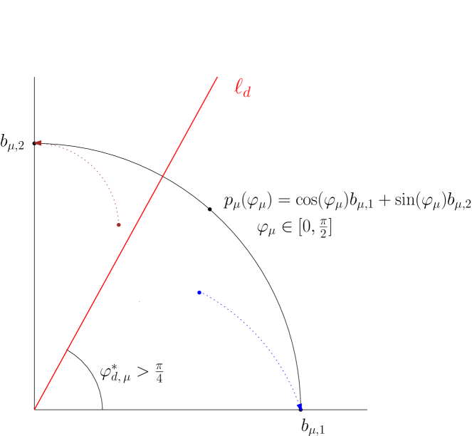
Figure 1: The angle $\varphi^{*}_{d,\,\mu}$ describes the slice where the global minimum is a point of attraction. Every initial guess located under the red line $\ell_{d}$ will converge to the global minimum. Note that the angle $\varphi^{*}_{d,\,\mu}$ is larger then $\frac{\pi}{4}$, but interestingly enough $\varphi^{*}_{d,\,\mu}\xrightarrow[d\rightarrow\infty]{}\frac{\pi}{4}$.

Example 1.3.

In the following example a sublinear convergence of ALS procedure for rank-one approximation is shown. We will consider the tensor $b_{\lambda}\in\mathcal{V}$ given by

$$b_{\lambda}=\bigotimes_{\mu=1}^{3}p+\lambda\left(p\otimes q\otimes q+q\otimes p\otimes q+q\otimes q\otimes p\right)$$

for some $\lambda\geq 0$ and $p,q\in\mathds{R}^{n}$ with $\|p\|=\|q\|=1$ and $\left\langle p,q\right\rangle=0$. Let us first prove the following statement.

Proposition 1.4.

Define $v^{*}:=\bigotimes_{\mu=1}^{3}p$. Then

a)

$\mathcal{M}_{b}=\{v^{*}\}$, if $\lambda\leq\frac{1}{2}$

b)

$|\mathcal{M}_{b}|=2$ and $v^{*}\notin\mathcal{M}_{b}$, if $\lambda>\frac{1}{2}$

Proof.

Let $v^{*}_{\lambda}\in\mathcal{M}_{b}$. Since tensor $b$ is symmetric, $v^{*}_{\lambda}$ also has to be symmetric. Write $v^{*}_{\lambda}=C_{\lambda}\bigotimes_{\mu=1}^{3}p_{\lambda}$, where $p_{\lambda}=p+\alpha_{\lambda}q$ (this is possible, since $\left\langle b,q\bigotimes q\bigotimes q\right\rangle=0$). Now the tuple $(C_{\lambda}p_{\lambda},p_{\lambda},p_{\lambda})$ is a stationary point of $F$, therefore

$$\left(\mbox{\bf Id}_{\mathds{R}^{n}}\otimes p_{\lambda}\otimes p_{\lambda}\right)^{T}b=Cp_{\lambda}$$

for some $C\in\mathds{R}$. But

$$\left(\mbox{\bf Id}_{\mathds{R}^{n}}\otimes p_{\lambda}\otimes p_{\lambda}\right)^{T}b=(1+\lambda\alpha_{\lambda}^{2})p+2\lambda\alpha_{\lambda}q,$$

hence

$$\frac{2\lambda\alpha_{\lambda}}{1+\lambda\alpha_{\lambda}^{2}}=\alpha_{\lambda}.$$ (10)

The solutions of (10) are

$$\alpha_{\lambda}=\left\{\begin{array}[]{ll}0,&\hbox{if $\lambda\leq\frac{1}{2}$,}\\ 0,\sqrt{\frac{2\lambda-1}{\lambda}}\text{ or }-\sqrt{\frac{2\lambda-1}{\lambda}},&\hbox{if $\lambda>\frac{1}{2}$.}\end{array}\right.$$

Straightforward calculations show that for $\lambda>\frac{1}{2}$ the solutions $\alpha_{\lambda}=\pm\sqrt{\frac{2\lambda-1}{\lambda}}$ lead to the same value of $F$ which is smaller than $f(v^{*})$. ∎

Now let $\lambda\leq\frac{1}{2}$ and $v_{k}=C^{k}p_{1}^{k}\otimes p_{2}^{k}\otimes\dots\otimes p_{d}^{k}$, with $p_{\mu}^{k}=c_{\mu}^{k}p+s_{\mu}^{k}q$, ${c_{\mu,k}}^{2}+{s_{\mu}^{k}}^{2}=1$ and some $C^{k}\in\mathds{R}$. Define $\gamma_{\mu,k}:=\left(\begin{array}[]{c}c_{\mu,k}\\ s_{\mu,k}\\ \end{array}\right)$. Applying Corollary 2.4, one gets after short calculations the recursion formula

$$\gamma_{1,k+1}=C_{1,k}M_{1,k}M_{1,k}^{T}\gamma_{1,k}$$

with some $C_{1,k}\in\mathds{R}$ and

$$M_{1,k}=\left(\begin{array}[]{cc}c_{2,k}&\lambda s_{2,k}\\ \lambda s_{2,k}&\lambda c_{2,k}\\ \end{array}\right).$$

Then for $t_{1,k}:=\frac{s_{1,k}}{c_{1,k}}$ it holds

$$t_{1,k+1}=\frac{\lambda(\lambda+1)c_{2,k}c_{1,k}\frac{s_{2,k}}{s_{1,k}}+\lambda^{2}}{c^{2}_{2,k}+\lambda^{2}s^{2}_{2,k}+\lambda(\lambda+1)\frac{c_{2,k}}{c_{1,k}}c_{2,k}s_{1,k}}\frac{s_{1,k}}{c_{1,k}}.$$ (11)

Thanks to Corollary 3.16 and Proposition 1.4 we know, that $\lim_{k\rightarrow\infty}v^{k}=v^{*}$ for $v^{*}=\bigotimes_{\mu=1}^{3}p$, therefore

$$\lim_{k\rightarrow\infty}c_{\mu,k}=1$$ (12)

$$\lim_{k\rightarrow\infty}s_{\mu,k}=0$$ (13)

for $\mu\in\mathds{N}_{3}$. From Eq. 12 and 11 one gets

$$\limsup_{k\rightarrow\infty}\frac{t_{1,k+1}}{t_{1,k}}=\lambda^{2}+\lambda(\lambda+1)\limsup_{k\rightarrow\infty}\frac{s_{2,k}}{s_{1,k}}.$$ (14)

The same way

$$\limsup_{k\rightarrow\infty}\frac{t_{2,k+1}}{t_{2,k}}=\lambda^{2}+\lambda(\lambda+1)\limsup_{k\rightarrow\infty}\frac{s_{3,k}}{s_{2,k}}$$ (15)

$$\limsup_{k\rightarrow\infty}\frac{t_{3,k+1}}{t_{3,k}}=\lambda^{2}+\lambda(\lambda+1)\limsup_{k\rightarrow\infty}\frac{s_{1,k+1}}{s_{3,k}}$$ (16)

Furthermore, from Eq. (21) we know that

$$p_{2,\,k+1}=C_{2,k+1}M_{2,k}p_{1,\,k+1}$$

with some $C_{2,k+1}\in\mathds{R}$ and

$$M_{2,k}=\left(\begin{array}[]{cc}c_{3,k}&\lambda s_{3,k}\\ \lambda s_{3,k}&\lambda c_{3,k}\\ \end{array}\right).$$

Simple calculations result in the relation

$$\frac{s_{2,k+1}}{s_{1,k+1}}=\lambda\frac{s_{3,k}}{s_{1,k+1}}c_{1,k+1}+\lambda c_{3,k},$$

and hence

$$\limsup_{k\rightarrow\infty}\frac{s_{2,k}}{s_{1,k}}=\lambda+\lambda\limsup_{k\rightarrow\infty}\frac{s_{3,k}}{s_{1,k+1}}$$ (17)

Now let $\lambda=\frac{1}{2}$. If $\limsup_{k\rightarrow\infty}\frac{s_{2,k}}{s_{1,k}}\geq 1$ , then from Eq. (14) follows $\limsup_{k\rightarrow\infty}\frac{t_{1,k+1}}{t_{1,k}}\geq 1$, hence the convergence of $p_{1,k}$ to $p$ can not be Q-linearly. If $\limsup_{k\rightarrow\infty}\frac{s_{2,k}}{s_{1,k}}<1$, then from Eq. (17) $\limsup_{k\rightarrow\infty}\frac{s_{1,k+1}}{s_{3,k}}\geq 1$, so from Eq. (15) $\limsup_{k\rightarrow\infty}\frac{t_{3,k+1}}{t_{3,k}}\geq 1$.

Remark 1.5.

• In fact for $\lambda=\frac{1}{2}$ it holds

  $$\limsup_{k\rightarrow\infty}\frac{s_{2,k}}{s_{1,k}}=\limsup_{k\rightarrow\infty}\frac{s_{3,k}}{s_{2,k}}=\limsup_{k\rightarrow\infty}\frac{s_{1,k+1}}{s_{3,k}}=1.$$

• For $\lambda<\frac{1}{2}$ ALS converges q-linearly with the convergence rate

  $$\rho=\frac{\lambda}{2}\left(3\lambda+\lambda^{2}+\sqrt{(3\lambda+\lambda^{2})^{2}+4\lambda}\right).$$

• The example can be extended to higher dimensions in the following way. Let

  $$b_{\lambda}=\bigotimes_{\mu=1}^{d}p+\lambda\sum_{\mu=1}^{d}\left(\bigotimes_{\nu=1}^{\mu-1}q\otimes p\otimes\bigotimes_{\nu=\mu+1}^{d}q\right)$$

  with $\|p\|=\|q\|$ and $\left\langle p,q\right\rangle=0$. Then $v^{*}=\bigotimes_{\mu=1}^{d}p$ is the unique best rank-one approximation of $b_{\lambda}$ if and only if $\lambda\leq\frac{1}{d-1}$. Furthermore, ALS converges sublinear for $\lambda=\frac{1}{d-1}$ and Q-linear for $\lambda<\frac{1}{d-1}$.

Our new convergence results are not obtained by using conventional technics like for the analysis of nonlinear Gauss-Seidel method or the theory of Lojasiewicz inequalities. Therefore, a detailed convergence approach is necessary.

2 The Alternating Least Squares Algorithm

In the following section, we recall the ALS algorithm. Where the algorithmic description of the ALS method is given in Algorithm 1.

Algorithm 1 Alternating Least Squares (ALS) Algorithm

1:  Set $k:=1$ and choose an initial guess $\underline{p}_{1}=(p^{1}_{1},\dots,p_{d}^{1})\in P$, $\underline{p}_{1,\,0}:=\underline{p}_{1}$, and $v_{1}:=U(\underline{p}_{1})\neq 0$.

2:  while Stop Condition do

3:     $v_{k,\,0}:=v_{k}$

4:     for ${1\leq\mu\leq d}$ do

5:        

$$p_{\mu}^{k+1} := \left(\frac{p_{1}^{k+1}}{\left\|p_{1}^{k+1}\right\|^{2}}\otimes\cdots\otimes\frac{p_{\mu-1}^{k+1}}{\left\|p_{\mu-1}^{k+1}\right\|^{2}}\otimes\mbox{\bf Id}_{\mathds{R}^{n_{\mu}}}\otimes\frac{p_{\mu+1}^{k}}{\left\|p_{\mu+1}^{k}\right\|^{2}}\otimes\cdots\otimes\frac{p_{d}^{k}}{\left\|p_{d}^{k}\right\|^{2}}\right)^{T}b$$ (18)

$$\underline{p}_{k,\mu+1} := (p_{1}^{k+1},\dots,\,p_{\mu-1}^{k+1}\,,p_{\mu}^{k+1},p_{\mu+1}^{k},\dots,p_{L}^{k})$$

$$v_{k,\mu+1} := U(\underline{p}_{k,\mu+1})$$

6:     end for

7:     $\underline{p}_{k+1}:=\underline{p}_{k,L}$ and $v_{k+1}:=U(\underline{p}_{k+1})$

8:     $k\mapsto k+1$

9:  end while

Notation 2.1 ($L(A,B)$, $P_{\nu,\mu}$).

Let $A,B$ be two arbitrary vector spaces. The vector space of linear maps from $A$ to $B$ is denoted by

$$L(A,B):=\left\{M:A\rightarrow B\,:\,M\mbox{ is linear}\right\}.$$

Let $\mu,\,\nu\in\mathds{N}_{d}$ with $\nu\neq\mu$. We define

$$P_{\nu,\mu}:=\mathds{R}^{n_{1}}\times\dots\times\mathds{R}^{n_{\nu-1}}\times\mathds{R}^{n_{\nu+1}}\times\dots\times\mathds{R}^{n_{\mu-1}}\times\mathds{R}^{n_{\mu+1}}\times\dots\times\mathds{R}^{n_{d}}.$$

The following map $M_{\mu,\nu}$ from Lemma 2.2 is important for the analytical understanding of the ALS algorithm. As Corollary 2.4 shows, the map $M_{\mu,{\mu-1}}$ describes an micro step of the ALS algorithm. Furthermore, there is an interesting relation between the map $M_{\mu,\nu}$ and rank-one best approximations of the tensor $b$, see Theorem 2.10.

Lemma 2.2.

Let $\mu,\nu\in\mathds{N}_{d}$, $\nu\neq\mu$, and $\underline{p}_{\nu,\,\mu}=(p_{1},\dots,p_{\nu-1},p_{\nu+1},\dots,p_{\mu-1},p_{\mu+1},\dots,p_{d})\in P_{\nu,\mu}$. There exists a multilinear map $M_{\nu,\mu}:P_{\nu,\mu}\times\mathcal{V}\rightarrow L(\mathds{R}^{n_{\nu}},\mathds{R}^{n_{\mu}})$ such that

$$M_{\nu,\mu}(\underline{p}_{\nu,\,\mu},b)\mathbf{g_{\nu}}=\left(p_{1}\otimes\dots\otimes p_{\nu-1}\otimes\mathbf{g_{\nu}}\otimes p_{\nu+1}\otimes\dots\otimes p_{\mu-1}\otimes\mbox{\bf Id}_{\mathds{R}^{n_{\mu}}}\otimes p_{\mu+1}\otimes\dots\otimes p_{d}\right)^{T}b$$ (19)

for all $\mathbf{g_{\nu}}\in\mathds{R}^{n_{\nu}}$. Further, we have $M_{\mu,\nu}(\underline{p}_{\nu,\,\mu},b)=M^{T}_{\nu,\mu}(\underline{p}_{\nu,\,\mu},b)$.

Proof.

Follows directly form the multilinearity of the tensor product and elementary calculations. ∎

Example 2.3.

Let $\mu,\nu\in\mathds{N}_{d}$, $\nu\neq\mu$, $\underline{p}_{\nu,\,\mu}=(p_{1},\dots,p_{\nu-1},p_{\nu+1},\dots,p_{\mu-1},p_{\mu+1},\dots,p_{d})\in P_{\nu,\mu}$, and $b$ be given in a subspace decomposition, i.e.

$$b = \sum_{i_{1}=1}^{t_{1}}\dots\sum_{i_{d}=1}^{t_{d}}\beta_{(i_{1},\dots,i_{d})}\bigotimes_{\mu=1}^{d}b_{\mu,i_{\mu}}\quad(t_{\mu}\in\mathds{N}_{n_{\mu}})$$

A matrix representation of the linear map $M_{\nu,\,\mu}$ is given by

$$M_{\nu,\mu}(\underline{p}_{\nu,\,\mu},b) = \sum_{i_{1}=1}^{t_{1}}\cdots\sum_{i_{\nu}=1}^{t_{\nu}}\cdots\sum_{i_{\mu}=1}^{t_{\mu}}\cdots\sum_{i_{d}=1}^{t_{d}}\beta_{(i_{1},\dots,i_{d})}\,\prod_{\xi\in\mathds{N}_{d}\setminus\{\mu,\,\nu\}}\left\langle b_{\xi,i_{\xi}},p_{\xi}\right\rangle\,b_{\mu,i_{\mu}}b^{T}_{\nu,i_{\nu}}$$

$$= B_{\mu}\Gamma(\underline{p}_{\nu,\,\mu})B_{\nu}^{T},$$

where $B_{\xi}=\left(b_{\xi,1},\dots,b_{\xi,t_{\xi}}\right)\in\mathds{R}^{n_{\xi}\times t_{\xi}}$ for all $\xi\in\{\mu,\nu\}$ and the entries of the matrix $\Gamma(\underline{p}_{\nu,\,\mu})$ are defined by

$$[\Gamma(\underline{p}_{\nu,\,\mu})]_{(i_{\nu},i_{\mu})}=\sum_{i_{1}=1}^{t_{1}}\cdots\sum_{i_{\nu-1}=1}^{t_{\nu-1}}\cdots\sum_{i_{\nu+1}=1}^{t_{\nu+1}}\cdots\sum_{i_{\mu-1}=1}^{t_{\mu-1}}\cdots\sum_{i_{\mu+1}=1}^{t_{\mu+1}}\cdots\sum_{i_{d}=1}^{t_{d}}\beta_{(i_{1},\dots,i_{d})}\,\prod_{\xi\in\mathds{N}_{d}\setminus\{\mu,\,\nu\}}\left\langle b_{\xi,i_{\xi}},p_{\xi}\right\rangle.$$

Corollary 2.4.

Let $\mu\in\mathds{N}_{d}$, $k\geq 2$, and $\underline{p}_{k,\mu}=(p^{k+1}_{1},\dots,p^{k+1}_{\mu-1},p_{\mu}^{k},p^{k}_{\mu+1},\dots,p_{d}^{k})\in P$ form Algorithm 1. With the matrix from Lemma 2.2, the following recursion formula holds:

$$p^{k+1}_{\mu} = \frac{1}{G_{k,\,\mu}G_{k,\,\mu-1}}M_{\mu,k}\,M^{T}_{\mu,k}\,\,p_{\mu}^{k},$$ (20)

where

$$G_{k,\,\mu} := \prod_{\nu=1}^{\mu-1}\left\|p_{\nu}^{k+1}\right\|^{2}\prod_{\nu=\mu+1}^{d}\left\|p_{\nu}^{k}\right\|^{2}$$

$$G_{k,\,\mu-1} := \prod_{\nu=1}^{\mu-2}\left\|p_{\nu}^{k+1}\right\|^{2}\prod_{\nu=\mu}^{d}\left\|p_{\nu}^{k}\right\|^{2},$$

$$M_{\mu,k} := M_{\mu,\mu-1}(p_{1}^{k+1},\dots,p_{\mu-2}^{k+1},p_{\mu+1}^{k},\dots,p_{d}^{k},b).$$

Proof.

We have with Eq. (18) and Lemma 2.2

$$p^{k+1}_{\mu} = \frac{1}{G_{k,\,\mu}}M_{\mu,\mu-1}(p_{1}^{k+1},\dots,p_{\mu-2}^{k+1},p_{\mu+1}^{k},\dots,p_{d}^{k},b)p_{\mu-1}^{k+1},$$ (21)

$$p_{\mu-1}^{k+1} = \frac{1}{G_{k,\,\mu-1}}M^{T}_{\mu,\mu-1}(p_{1}^{k+1},\dots,p_{\mu-2}^{k+1},p_{\mu+1}^{k},\dots,p_{d}^{k},b)p_{\mu}^{k}.$$ (22)

∎

Example 2.5.

Let $v_{k}=p_{1}^{k}\otimes p_{2}^{k}\otimes\dots\otimes p_{d}^{k}$ and

$$b=\sum_{i_{1}=1}^{t_{1}}\dots\sum_{i_{d}=1}^{t_{d}}\beta_{(i_{1},\dots,i_{d})}\bigotimes_{\mu=1}^{d}b_{\mu,i_{\mu}},$$

i.e. the tensor $b$ is given in the Tucker decomposition. From Eq. (18) it follows

$$p_{1}^{k+1} = \frac{1}{\prod_{\mu=2}^{d}\left\|p_{\mu}^{k}\right\|^{2}}\sum_{i_{1}=1}^{t_{1}}\dots\sum_{i_{d}=1}^{t_{d}}\beta_{(i_{1},\dots,i_{d})}\prod_{\mu=2}^{d}\left\langle b_{\mu,i_{\mu}},p_{\mu}^{k}\right\rangle b_{1,i_{1}}$$

$$= \frac{1}{\prod_{\mu=2}^{d-1}\left\|p_{\mu}^{k}\right\|\|p_{d}^{k}\|^{2}}\left[\sum_{i_{1}=1}^{t_{1}}\sum_{i_{d}=1}^{t_{d}}b_{1,i_{1}}\sum_{i_{2}=1}^{t_{2}}\dots\sum_{i_{d-1}=1}^{t_{d-1}}\beta_{(i_{1},\dots,i_{d})}\prod_{\mu=2}^{d-1}\frac{\left\langle b_{\mu,i_{\mu}},p_{\mu}^{k}\right\rangle}{\|p_{\mu}^{k}\|}b^{T}_{d,i_{d}}\right]p_{d}^{k}$$

$$= \frac{1}{\prod_{\mu=2}^{d-1}\left\|p_{\mu}^{k}\right\|\|p_{d}^{k}\|^{2}}B_{1}\Gamma_{1,k}B_{d}^{T}p_{d}^{k},$$

where $B_{\mu}=\left(b_{\mu,i_{\mu}}\,:\,1\leq i_{\mu}\leq t_{\mu}\right)\in\mathds{R}^{n_{\mu}\times t_{\mu}}$, $B_{\mu}^{T}B_{\mu}=\mbox{\bf Id}_{\mathds{R}^{t_{\mu}}}$, and the entries of the matrix $\Gamma_{1,k}\in\mathds{R}^{t_{1}\times t_{d}}$ are defined by

$$[\Gamma_{1,k}]_{i_{1},i_{d}}=\sum_{i_{2}=1}^{t_{2}}\dots\sum_{i_{d-1}=1}^{t_{d-1}}\beta_{(i_{1},\dots,i_{d})}\prod_{\mu=2}^{d-1}\frac{\left\langle b_{\mu,i_{\mu}},p_{\mu}^{k}\right\rangle}{\|p_{\mu}^{k}\|}\quad\left(1\leq i_{1}\leq t_{1},\,1\leq i_{d}\leq t_{d}\right).$$

Note that $\Gamma_{1,k}$ is a diagonal matrix if the coefficient tensor $\beta\in\bigotimes_{\mu=1}^{d}\mathds{R}^{t_{\mu}}$ is super- diagonal, see Eq. (6). For $p_{d}^{k}$ it follows further

$$p_{d}^{k} = \frac{1}{\prod_{\mu=1}^{d-1}\left\|p_{\mu}^{k}\right\|^{2}}\sum_{i_{1}=1}^{t_{1}}\dots\sum_{i_{d}=1}^{t_{d}}\beta_{(i_{1},\dots,i_{d})}\prod_{\mu=1}^{d-1}\left\langle b_{\mu,i_{\mu}},p_{\mu}^{k}\right\rangle b_{d,i_{d}}=\frac{1}{\left\|p_{1}^{k}\right\|^{2}\prod_{\mu=2}^{d-1}\left\|p_{\mu}^{k}\right\|}B_{d}\Gamma^{T}_{1,k}B_{1}^{T}p_{1}^{k}$$

and finally

$$p_{1}^{k+1}=\frac{1}{\prod_{\mu=1}^{d}\left\|p_{\mu}^{k}\right\|^{2}}\,B_{1}\Gamma_{1,k}\Gamma^{T}_{1,k}B_{1}^{T}\,p_{1}^{k}.$$

Let $v^{*}=\lambda\,p_{1}\otimes\dots\otimes p_{d}\in\mathcal{M}_{b}$ be a rank-one best approximation of $b$. Without loss of generality we can assume that

$$\|p_{1}\|=\|p_{2}\|=\cdots=\|p_{d}\|=1\mbox{ and }\|v^{*}\|=\lambda.$$

Further, let $\mu,\nu\in\mathds{N}_{d}$ and

$$\underline{p}_{\nu,\,\mu}:=(p_{1},\dots,p_{\nu-1},p_{\nu+1},\dots,p_{\mu-1},p_{\mu+1},\dots,p_{d})\in P_{\nu,\mu}.$$

The following two maps are of interest for our analysis:

$$\bar{V}:S^{n_{\nu}-1}\times S^{n_{\mu}-1} \rightarrow \mathcal{V}$$

$$(g_{\nu},g_{\mu}) \mapsto \bar{V}(g_{\nu},g_{\mu}):=p_{1}\otimes\cdots\otimes p_{\nu-1}\otimes g_{\nu}\otimes p_{\nu+1}\otimes\cdots\otimes p_{\mu-1}\otimes g_{\mu}\otimes p_{\mu+1}\otimes\cdots\otimes p_{d}$$

and

$$\bar{U}:S^{n_{\nu}-1}\times S^{n_{\mu}-1} \rightarrow \mathcal{V}$$

$$(g_{\nu},g_{\mu}) \mapsto \bar{U}(g_{\nu},g_{\mu}):=\left\langle\bar{V}(g_{\nu},g_{\mu}),b\right\rangle\bar{V}(g_{\nu},g_{\mu}),$$

where $S^{n-1}=\{x\in\mathds{R}^{n}:\|x\|=1\}$ denotes the sphere in $\mathds{R}^{n}$.

Lemma 2.6.

Let $\mu,\nu\in\mathds{N}_{d}$, $g_{\nu}\in S^{n_{\nu}-1}$ and $g_{\mu}\in S^{n_{\mu}-1}$. We have

$$-2f\left(\bar{U}(g_{\nu},g_{\mu})\right) = \left\langle\underbrace{\left(M_{\nu,\mu}(\underline{p}_{\nu,\,\mu},b)\right)}_{\in L(\mathds{R}^{n_{\nu}},\mathds{R}^{n_{\mu}})}g_{\nu},g_{\mu}\right\rangle^{2}=\left\langle\bar{U}(g_{\nu},g_{\mu}),b\right\rangle=\left\|\bar{U}(g_{\nu},g_{\mu})\right\|^{2}.$$

Proof.

Let $g_{\nu}\in S^{n_{\nu}-1}$, $g_{\mu}\in S^{n_{\mu}-1}$, and define $\pi(g_{\nu},g_{\mu}):=\bar{V}(g_{\nu},g_{\mu})(\bar{V}(g_{\nu},g_{\mu}))^{T}$. It holds $\bar{U}(g_{\nu},g_{\mu})=\pi(g_{\nu},g_{\mu})b$ and

$$f\left(\bar{U}(g_{\nu},g_{\mu})\right) = \frac{1}{2}\left\langle\bar{U}(g_{\nu},g_{\mu}),\bar{U}(g_{\nu},g_{\mu})\right\rangle-\left\langle\bar{U}(g_{\nu},g_{\mu}),b\right\rangle=\frac{1}{2}\left\langle\pi^{2}(g_{\nu},g_{\mu})b,b\right\rangle-\left\langle\pi(g_{\nu},g_{\mu})b,b\right\rangle$$

$$= \frac{1}{2}\left\langle\pi(g_{\nu},g_{\mu})b,b\right\rangle-\left\langle\pi(g_{\nu},g_{\mu})b,b\right\rangle=-\frac{1}{2}\left\langle\pi(g_{\nu},g_{\mu})b,b\right\rangle=-\frac{1}{2}\left\langle\bar{U}(g_{\nu},g_{\mu}),b\right\rangle$$

$$= -\frac{1}{2}\left\langle\pi^{2}(g_{\nu},g_{\mu})b,b\right\rangle=-\frac{1}{2}\left\langle\pi(g_{\nu},g_{\mu})b,\pi(g_{\nu},g_{\mu})b\right\rangle=-\frac{1}{2}\left\|\bar{U}(g_{\nu},g_{\mu})\right\|^{2}$$

$$= -\frac{1}{2}\left\langle\bar{V}(g_{\nu},g_{\mu}),b\right\rangle^{2}=-\frac{1}{2}\left\langle\left(M_{\nu,\mu}(\underline{p}_{\nu,\,\mu},b)\right)g_{\nu},g_{\mu}\right\rangle^{2}.$$

∎

Remark 2.7.

Obviously, the minimisation problem from Eg. (3) is equivalent to the following constrained maximisation problem: Find $\tilde{v}=\bigotimes_{\mu=1}^{d}p_{\mu}$ such that for all $\mu\in\mathds{N}_{d}$ it holds

$$\left\langle\tilde{v},b\right\rangle=\max_{v\in U(P)}\left\langle v,b\right\rangle\quad\mbox{subject to }\|p_{\mu}\|=1.$$

Lagrangian method for constrained optimisation leads to

$$L_{\underline{\lambda}}(q_{1},\cdots,q_{d})=\left\langle U(q_{1},\cdots,q_{d}),b\right\rangle+\frac{1}{2}\sum_{\mu=1}^{d}\lambda_{\mu}\left(1-\|q_{\mu}\|^{2}\right),$$

where $q_{\mu}\in\mathds{R}^{n_{\mu}}$ and $\underline{\lambda}=(\lambda_{1},\cdots,\lambda_{d})^{T}\in\mathds{R}^{d}$ is the vector of Lagrange multipliers. A rank-one best approximation $v^{*}=\lambda\,p_{1}\otimes\cdots\otimes p_{d}\in\mathcal{M}_{b}$ with $\lambda\in\mathds{R}$ and $\|p_{\mu}\|=1$ satisfies

$$\frac{\partial}{\partial p_{\mu}}L_{\underline{\lambda}^{*}}(p_{1},\cdots,p_{d}) = \left(p_{1}\otimes\cdots p_{\mu-1}\otimes\mbox{\bf Id}_{\mathds{R}^{n_{\mu}}}\otimes p_{\mu+1}\otimes\cdots\otimes p_{d}\right)^{T}b-\lambda^{*}_{\mu}p_{\mu}=0,$$

$$\frac{\partial}{\partial\lambda^{*}_{\mu}}L_{\underline{\lambda}^{*}}(p_{1},\cdots,p_{d}) = \frac{1}{2}\left(1-\|p_{\mu}\|^{2}\right)=0.$$

For $\nu\in\mathds{N}_{d}\setminus\{\mu\}$ it follows that

$$\lambda = \left\langle p_{1}\otimes\cdots\otimes p_{d},b\right\rangle,\quad\lambda\,p_{\mu}=M_{\nu,\mu}(\underline{p}_{\nu,\,\mu},b)\,p_{\nu},\quad\lambda\,p_{\nu}=M^{T}_{\nu,\mu}(\underline{p}_{\nu,\,\mu},b)\,p_{\mu},$$

where $\underline{p}_{\nu,\mu}\in P_{\nu,\mu}$ is like in Lemma 2.2. Therefore, $\lambda$ is a singular value of the matrix $M_{\nu,\mu}(\underline{p}_{\nu,\,\mu},b)$ and $p_{\nu},\,p_{\mu}$ are the associated singular vectors.

Proposition 2.8.

Let $v^{*}=\lambda p_{1}\otimes\cdots\otimes p_{d}\in\mathcal{M}_{b}$ a best approximation of $b$ with $\|p_{1}\|=\cdots=\|p_{d}\|=1$. We have

$$f(v^{*})=-\frac{1}{2\,\|b\|^{2}}\|v^{*}\|^{2}=-\frac{1}{2\,\|b\|^{2}}\left\langle b,v^{*}\right\rangle.$$

Proof.

Since $v^{*}\in\mathcal{M}_{b}$ we have that $v^{*}=\Pi b$, where $\Pi:=\frac{v^{*}{v^{*}}^{T}}{\|v^{*}\|^{2}}$. Furthermore, it holds

$$\left\langle v^{*},v^{*}\right\rangle = \left\langle\Pi b,v^{*}\right\rangle=\left\langle b,\Pi v^{*}\right\rangle=\left\langle b,v^{*}\right\rangle.$$

The rest follows from the definition of $f$, see Eq. (1). ∎

Remark 2.9.

From Proposition 2.8 it follows instantly that the global minimum of the best approximation problem from Eq. (3) has the largest norm among all other $\tilde{v}\in\mathcal{M}_{b}$.

Theorem 2.10.

Let $\mu,\nu\in\mathds{N}_{d}$ and $v^{*}=\|v^{*}\|p_{1}\otimes\dots\otimes p_{d}\in\mathcal{M}_{b}$ be a rank-one best approximation of $b$ with $\|p_{1}\|=\cdots=\|p_{d}\|=1$. Then $\|v^{*}\|$ is the largest singular value of $M_{\nu,\mu}(\underline{p}_{\nu,\,\mu},b)$ and $p_{\nu},\,p_{\mu}$ are the associated singular vectors. Furthermore, if $v^{*}$ is isolated, then $\|v^{*}\|$ is a simple singular value of $M_{\nu,\mu}(\underline{p}_{\nu,\,\mu},b)$.

Proof.

Let $\mu,\,\nu\in\mathds{N}_{d}$. From Lemma 2.6 and Remark 2.7 it follows that $\|v^{*}\|$ is a singular value of $M_{\nu,\mu}(\underline{p}_{\nu,\,\mu},b)$ and $p_{\nu},\,p_{\mu}$ are associated singular vectors. Assume that there is a singular value $\tilde{\lambda}$ of $M_{\nu,\mu}(\underline{p}_{\nu,\,\mu},b)$ and associated singular vectors $q_{\nu}\in\mathds{R}^{n_{\nu}},q_{\mu}\in\mathds{R}^{n_{\mu}}$ with $\tilde{\lambda}>\|v^{*}\|$. Let $\alpha\in[0,1]$ and $\beta\in(0,1]$ with $\alpha^{2}+\beta^{2}=1$. Define further $g_{\nu}(\alpha,\beta):=g_{\nu}:=\alpha p_{\nu}+\beta q_{\nu}\in\mathds{R}^{n_{\nu}}$ and $g_{\mu}(\alpha,\beta):=g_{\mu}:=\alpha p_{\mu}+\beta q_{\mu}\in\mathds{R}^{n_{\mu}}$. We have $\|g_{\nu}\|^{2}=\|g_{\mu}\|^{2}=\alpha^{2}+\beta^{2}=1$ and with Lemma 2.6 it follows then

$$-2f(\bar{U}(g_{\nu},g_{\mu})) = \left\langle\left(M_{\nu,\mu}(\underline{p}_{\nu,\,\mu},b)\right)g_{\nu},g_{\mu}\right\rangle^{2}=\left\langle\left(M_{\nu,\mu}(\underline{p}_{\nu,\,\mu},b)\right)\alpha p_{\nu}+\beta q_{\nu},\alpha p_{\mu}+\beta q_{\mu}\right\rangle^{2}$$

$$= \left\langle\alpha\|v^{*}\|p_{\nu}+\beta\tilde{\lambda}q_{\nu},\alpha p_{\mu}+\beta q_{\mu}\right\rangle^{2}=\left(\alpha^{2}\|v^{*}\|+\beta^{2}\tilde{\lambda}\right)^{2}$$

$$\overset{(\beta\neq 0)}{>} \left(\alpha^{2}\|v^{*}\|+\beta^{2}\|v^{*}\|\right)^{2}=\|v^{*}\|^{2}=\left\langle\left(M_{\nu,\mu}(\underline{p}_{\nu,\,\mu},b)\right)p_{\nu},p_{\mu}\right\rangle^{2}=-2f(v^{*}).$$

Consequently, it is

$$f(\bar{U}(g_{\nu}(\alpha,\beta),g_{\mu}(\alpha,\beta)))<f(v^{*})\quad\mbox{for all }\alpha\in[0,1]\mbox{ and }\beta\in(0,1]\mbox{ with }\alpha^{2}+\beta^{2}=1,$$

i.e. we can finde a better approximation $\bar{U}(g_{\nu}(\alpha,\beta),g_{\mu}(\alpha,\beta))$ of $b$ which is arbitrary close to $v^{*}$. This contradicts the fact that $v^{*}\in\mathcal{M}_{b}$.
Additionally, let $v^{*}$ be a isolated rank-one best approximation of $b$. Assume that there is a singular value $\lambda$ of $M_{\nu,\mu}(\underline{p}_{\nu,\,\mu},b)$ and associated singular vectors $q_{\nu}\in\mathds{R}^{n_{\nu}},\,q_{\mu}\in\mathds{R}^{m_{\mu}}$ with $\lambda=\|v^{*}\|$, $p_{\nu}\bot q_{\nu}$, and $p_{\mu}\bot q_{\mu}$. Almost like above, let $\alpha,\,\beta\in[0,1]$ with $\alpha^{2}+\beta^{2}=1$ and consider again $g_{\nu}(\alpha,\beta)=\alpha p_{\nu}+\beta q_{\nu}\in\mathds{R}^{n_{\nu}}$, $g_{\mu}(\alpha,\beta)=\alpha p_{\mu}+\beta q_{\mu}\in\mathds{R}^{n_{\mu}}$. With Lemma 2.6 it follows

$$-2f(\bar{U}(g_{\nu},g_{\mu})) = \left(\alpha^{2}\|v^{*}\|+\beta^{2}\lambda\right)^{2}=\|v^{*}\|^{2}=\left\langle\left(M_{\nu,\mu}(\underline{p}_{\nu,\,\mu},b)\right)p_{\nu},p_{\mu}\right\rangle^{2}=-2f(v^{*}),$$

i.e. we have

$$f(\bar{U}(g_{\nu}(\alpha,\beta),g_{\mu}(\alpha,\beta)))=f(v^{*})\quad\mbox{for all }\alpha,\,\beta\in[0,1]\mbox{ with }\alpha^{2}+\beta^{2}=1.$$

Therefore, we can finde a approximation $\bar{U}(g_{\nu}(\alpha,\beta),g_{\mu}(\alpha,\beta))$ of $b$ which is arbitrary close to $v^{*}$ and $f(\bar{U}(g_{\nu}(\alpha,\beta),g_{\mu}(\alpha,\beta)))=f(v^{*})$. This contradicts the fact that $v^{*}$ is isolated. ∎

Remark 2.11.

The proof of Theorem 2.10 shows that if we have two different best approximations of $b$ which differ only in two arbitrary components of the representation systems and $f(v^{*})=f(v^{**})$, then there is a complete path between $v^{*}$ and $v^{**}$ described by $\bar{U}(g_{\nu}(\alpha,\beta),g_{\mu}(\alpha,\beta))$ such that $f(v^{*})=f\left(\bar{U}(g_{\nu}(\alpha,\beta),g_{\mu}(\alpha,\beta))\right)$.

3 Convergence Analysis

In the following, we are using the notations and definitions from Section 2. Our convergence analysis is mainly based on the recursion introduced in Corollary 2.4 and the following Lemma 3.1.

Lemma 3.1.

Let $k\in\mathds{N}$, $\mu\in\mathds{N}$, and $v_{k,\mu}=p_{1}^{k+1}\otimes\cdots\otimes p_{\mu-1}^{k+1}\otimes p_{\mu}^{k}\otimes\cdots\otimes p_{d}^{k}$ from Algorithm 1. Then

$$\Pi_{k,\mu}:=\frac{p_{1}^{k+1}\left(p_{1}^{k+1}\right)^{T}}{\left\|p_{1}^{k+1}\right\|^{2}}\otimes\cdots\otimes\frac{p_{\mu-1}^{k+1}\left(p_{\mu-1}^{k+1}\right)^{T}}{\left\|p_{\mu-1}^{k+1}\right\|^{2}}\otimes\mbox{\bf Id}_{\mathds{R}^{n_{\mu}}}\otimes\frac{p_{\mu+1}^{k}\left(p_{\mu+1}^{k}\right)^{T}}{\left\|p_{\mu+1}^{k}\right\|^{2}}\otimes\cdots\otimes\frac{p_{d}^{k+1}\left(p_{d}^{k+1}\right)^{T}}{\left\|p_{d}^{k+1}\right\|^{2}}$$

is a orthogonal projection and

$$v_{k,\mu+1}=v_{k,\mu}+\Pi_{k,\mu}r_{k,\mu},$$

where $r_{k,\mu}:=b-v_{k,\mu}$.

Proof.

Obviously, $\Pi_{k,\mu}$ is a orthogonal projection. Straightforward calculations show that $v_{k,\mu}=\Pi_{k,\mu}v_{k,\mu}$ and $v_{k,\mu+1}=\Pi_{k,\mu}b$. Hence we have $v_{k,\mu}+\Pi_{k,\mu}r_{k,\mu}=\Pi_{k,\mu}b=v_{k,\mu+1}$. ∎

Lemma 3.2.

Let $k\in\mathds{N}$, $\mu\in\mathds{N}_{L}$. We have

$$f(v_{k,\,\mu})-f(v_{k,\mu+1})=\frac{1}{2}\frac{\left\langle\Pi_{k,\mu}r_{k,\mu},r_{k,\mu}\right\rangle}{\|b\|^{2}}$$ (23)

Proof.

It follows with Lemma 3.1 that

$$f(v_{k,\mu+1}) = \frac{1}{\|b\|^{2}}\left[\frac{1}{2}\left\langle v_{k,\mu}+\Pi_{k,\mu}r_{k,\mu},v_{k,\mu}+\Pi_{k,\mu}r_{k,\mu}\right\rangle-\left\langle b,v_{k,\mu}+\Pi_{k,\mu}r_{k,\mu}\right\rangle\right]$$

$$= f(v_{k,\mu})+\frac{1}{\|b\|^{2}}\left[\frac{1}{2}\left\langle\Pi_{k,\mu}r_{k,\mu},\Pi_{k,\mu}r_{k,\mu}\right\rangle+\left\langle v_{k,\mu},\Pi_{k,\mu}r_{k,\mu}\right\rangle-\left\langle b,\Pi_{k,\mu}r_{k,\mu}\right\rangle\right]$$

$$= f(v_{k,\mu})+\frac{1}{\|b\|^{2}}\left[\frac{1}{2}\left\langle r_{k,\mu},\Pi_{k,\mu}r_{k,\mu}\right\rangle-\left\langle r_{k,\mu},\Pi_{k,\mu}r_{k,\mu}\right\rangle\right]$$

$$= f(v_{k,\mu})-\frac{1}{2}\frac{\left\langle\Pi_{k,\mu}r_{k,\mu},r_{k,\mu}\right\rangle}{\|b\|^{2}},$$

i.e. $f(v_{k,\,\mu})-f(v_{k,\mu+1})=\frac{1}{2}\frac{\left\langle\Pi_{k,\mu}r_{k,\mu},r_{k,\mu}\right\rangle}{\|b\|^{2}}$. ∎

Corollary 3.3.

There exists $\alpha\in\mathds{R}$ such that $f(v_{k})\xrightarrow[k\rightarrow\infty]{}\alpha$.

Proof.

Let $k\in\mathds{N}$ and $\mu\in\mathds{N}_{L}$. From Lemma 3.2 and Lemma 3.1 it follows that

$$f(v_{k+1})-f(v_{k}) = f(v_{k,d})-f(v_{k,0})=\sum_{\mu=1}^{d}f(v_{k,\,\mu})-f(v_{k,\mu-1})$$

$$= -\frac{1}{2\|b\|^{2}}\sum_{\mu=0}^{d-1}\left\|\Pi_{k,\mu}r_{k,\mu}\right\|^{2}\leq 0,$$

This shows that $(f(v_{k}))_{k\in\mathds{N}}\subset\mathds{R}$ is a descending sequence. The sequence of function values $(f(v_{k}))_{k\in\mathds{N}}$ is bounded from below. Therefore, there exist an $\alpha\in\mathds{R}$ such that $f(v_{k})\xrightarrow[k\rightarrow\infty]{}\alpha$. ∎

Remark 3.4.

From the definition of the ALS method it is already clear that $(f(v_{k,\mu}))_{\mu\in\mathds{N}_{d},k\in\mathds{N}}$ is a descending sequence.

Lemma 3.5.

Let $(v_{k,\mu})_{k\in\mathds{N},\mu\in\mathds{N}_{d}}\subset\mathcal{V}$ be the sequence from Algorithm 1. We have

$$f(v_{k,\mu})=-\frac{1}{2\|b\|^{2}}\left\langle v_{k,\mu},b\right\rangle=-\frac{1}{2\|b\|^{2}}\|v_{k,\mu}\|^{2}$$ (24)

for all $k\in\mathds{N},\mu\in\mathds{N}_{d}$.

Proof.

Let $k\in\mathds{N}$ and $\mu\in\mathds{N}_{d}$. With Lemma 3.1 it follows

$$\left\langle v_{k,\mu},v_{k,\mu}\right\rangle = \left\langle\Pi_{k,\mu-1}b,\Pi_{k,\mu-1}b\right\rangle=\left\langle\Pi^{2}_{k,\mu-1}b,b\right\rangle=\left\langle\Pi_{k,\mu-1}b,b\right\rangle=\left\langle v_{k,\mu},b\right\rangle.$$

The rest follows from the definition of $f$, see Eq. (1). ∎

Corollary 3.6.

Let $(v_{k,\mu})_{k\in\mathds{N},\mu\in\mathds{N}_{d}}\subset\mathcal{V}$ be the sequence of represented tensors from the ALS algorithm. Further, let $\mu\in\mathds{N}_{d}$ and $k\in\mathds{N}$. The following statements are equivalent:

• $f(v_{k,\mu+1})\leq f(v_{k,\mu})$

• $\|v_{k,\mu+1}\|^{2}\geq\|v_{k,\mu}\|^{2}$

• $\|p^{k+1}_{\mu}\|^{2}\geq\|p^{k}_{\mu}\|^{2}$

• $\cos^{2}(\varphi_{k,\mu+1})\geq\cos^{2}(\varphi_{k,\mu})$, where $\cos^{2}(\varphi_{k,\mu}):=\frac{\left\langle\Pi_{k,\mu}b,b\right\rangle}{\|b\|^{2}}$.

Proof.

Follows direct from Lemma 3.5 and

$$\|v_{k,\mu+1}\|^{2}\geq\|v_{k,\mu}\|^{2}\Leftrightarrow G_{k,\mu}\|p^{k+1}_{\mu}\|^{2}\geq G_{k,\mu}\|p^{k}_{\mu}\|^{2}$$

where $G_{k,\mu}>0$ is defined in Corollary 2.4. ∎

Lemma 3.7.

Let $(v_{k})_{k\in\mathds{N}}\subset\mathcal{V}$ be the sequence of represented tensors from the ALS method. It holds

$$\|v_{k+1}-v_{k}\|\xrightarrow[k\rightarrow\infty]{}0.$$

Proof.

Let $k\in\mathds{N}$. We have

$$\|v_{k+1}-v_{k}\|^{2} = \left\|\sum_{\mu=1}^{d}v_{k,\mu}-v_{k,\mu-1}\right\|^{2}\leq\left(\sum_{\mu=1}^{d}\|v_{k,\mu}-v_{k,\mu-1}\|\right)^{2}\leq d\sum_{\mu=0}^{d-1}\left\|v_{k,\mu+1}-v_{k,\mu}\right\|^{2}.$$ (25)

Since $v_{k,\mu+1}-v_{k,\mu}=\Pi_{k,\mu}r_{k,\mu}$, see Lemma 3.1, it follows further with Eq. (23) and (25) that

$$\|v_{k+1}-v_{k}\|^{2} \leq 2d\|b\|^{2}\sum_{\mu=0}^{d-1}\left(f(v_{k,\mu+1})-f(v_{k,\mu})\right).$$

With Corollary 3.3 we have $\left(f(v_{k,\mu+1})-f(v_{k,\mu})\right)\xrightarrow[k\rightarrow\infty]{}0$, hence $\|v_{k+1}-v_{k}\|\xrightarrow[k\rightarrow\infty]{}0$. ∎

Definition 3.8 ($\mathcal{A}(v_{k})$, critical points).

Let $(v_{k})_{k\in\mathds{N}}\subset\mathcal{V}$ be the sequence of represented tensors from Algorithm 1. The set of accumulation points of $(v_{k})_{k\in\mathds{N}}$ is denoted by $\mathcal{A}(v_{k})$, i.e.

$$\mathcal{A}(v_{k}):=\left\{v\in\mathcal{V}:v\mbox{ is an accumulation point of }(v_{k})_{k\in\mathds{N}}\right\}.$$ (26)

The set $\mathfrak{M}$ of critical points of the optimisation problem from Eq. (2) is defined as follows:

$$\mathfrak{M}:=\left\{v\in\mathcal{V}\,:\,\exists\underline{p}\in P:v=U(\underline{p})\wedge F^{\prime}(\underline{p})=0\right\}.$$ (27)

Proposition 3.9.

The sequence of parameter $(p_{\mu,k})_{\mu\in\mathds{N}_{d},k\in\mathds{N}}$ from the ALS algorithm is bounded.

Proof.

From the definition of $f$ and Lemma 3.5 it follows that

$$-\frac{1}{2}\leq f(v_{k,\mu})=-\frac{1}{2}\frac{\|v_{k,\mu}\|^{2}}{\|b\|^{2}}\quad\Leftrightarrow\quad\|v_{k,\mu}\|\leq\|b\|,$$

i.e. the sequence $(\|v_{\mu,k}\|)_{\mu\in\mathds{N}_{d},k\in\mathds{N}}\subset\mbox{\rm Range$\,$}(U)$ is bounded. The sequence $(\|v_{\mu,k}\|)_{\mu\in\mathds{N}_{d},k\in\mathds{N}}$ is the product of the following $d$ sequences $(\|p_{\mu}^{k}\|)_{k\in\mathds{N}}\subset\mathds{R}^{n_{\mu}}$. According to Corollary 3.6 the sequences $(\|p_{\mu}^{k}\|)_{k\in\mathds{N}}$ are monotonically increasing. Since the product $\|v_{\mu,k}\|$ is bounded and all sequences $(\|p_{\mu}^{k}\|)_{k\in\mathds{N}}$ are monotonically increasing, it follows that all $(p_{\mu}^{k})_{k\in\mathds{N}}$ are bounded. This means the sequence $(p_{\mu,k})_{\mu\in\mathds{N}_{d},k\in\mathds{N}}$ is bounded. ∎

The following statements are proofed in a corresponding article about the convergence of alternating least squares optimisation in general tensor format representations, please see [5] for more informations regarding the proofs.

Lemma 3.10 ([5]).

We have

$$\max_{0\leq\mu\leq L-1}\left\|F_{\mu}^{\prime}(p_{\mu}^{k})\right\|\xrightarrow[k\rightarrow\infty]{}0.$$

Corollary 3.11 ([5]).

Let $(\underline{p}_{k})_{k\in\mathds{N}}$ be the sequence from Algorithm 1 and $F:P\rightarrow\mathds{R}$ from Eq. (2). We have

$$\lim_{k\rightarrow\infty}F^{\prime}(\underline{p}_{k})=0.$$

Theorem 3.12 ([5]).

Let $(v_{k})_{k\in\mathds{N}}$ be the sequence of represented tensors from the ALS method. Every accumulation point of $(v_{k})_{k\in\mathds{N}}$ is a critical point, i.e. $\mathcal{A}(v_{k})\subseteq\mathfrak{M}$. Further, we have

$$\mbox{\rm dist$\,$}\left(v_{k},\mathfrak{M}\right)\xrightarrow[k\rightarrow\infty]{}0.$$

Let $\bar{v}\in\mathfrak{M}$ be a critical point and $N:=\prod_{\mu=1}^{d}n_{\mu}\in\mathds{N}$. Further, let $(\underline{p}_{k,\mu})_{k\in\mathds{N},\mu\in\mathds{N}_{d}}\subset P$ be the sequence of parameter from the ALS algorithm and $R\in\mathds{R}^{N\times N-1}$ be a matrix with $R^{T}R=\mbox{\bf Id}_{\mathds{R}^{N-1}}$ and $\mbox{\rm span}(\bar{v})^{\bot}=\mbox{\rm Range$\,$}(R)$, i.e. the column vectors of $R$ build an orthonormal basis of the linear space $\mbox{\rm span}(\bar{v})^{\bot}$. Then the block matrix

$$V:=\left[\begin{array}[]{cc}\underline{v}&R\\ \end{array}\right]\in\mathds{R}^{N\times N},\quad\left(\,\underline{v}:=\bar{v}/\|\bar{v}\|\,\right).$$ (28)

is orthogonal, i.e. the columns of the matrix $V$ build an orthonormal basis of the tensor space $\mathcal{V}$. The following matrix $N_{k,\mu}\in\mathds{R}^{N\times N}$ is imported in order to describe the rate of convergence for the ALS method:

$$N_{k,\mu}:=\bigotimes_{\nu=1}^{\mu-1}\mbox{\bf Id}\otimes\left(\frac{1}{G_{k,\,\mu}G_{k,\,\mu-1}}M_{\mu,k}\,M^{T}_{\mu,k}\right)\otimes\bigotimes_{\nu=\mu+1}^{d}\mbox{\bf Id},$$

where the matrix $\frac{1}{G_{k,\,\mu}G_{k,\,\mu-1}}M_{\mu,k}\,M^{T}_{\mu,k}$ is from Corollary 2.4. Further, it follows from Corollary 2.4 that for the ALS micro step the following equation:

$$v_{k,\mu+1}=N_{k,\mu}v_{k,\mu}$$ (29)

holds. The tensor $v_{k,\mu}$ and the matrix $N_{k,\mu}$ are represented with respect to the basis $V$, i.e

$$v_{k,\mu} = VV^{T}v_{k,\mu}=\left[\begin{array}[]{cc}\underline{v}&R\\ \end{array}\right]\left(\begin{array}[]{c}\underbrace{\underline{v}^{T}v_{k,\mu}}_{c_{k,\mu}:=}\\ \underbrace{R^{T}v_{k,\mu}}_{s_{k,\mu}:=}\\ \end{array}\right)=\left[\begin{array}[]{cc}\underline{v}&R\\ \end{array}\right]\left(\begin{array}[]{c}c_{k,\mu}\\ s_{k,\mu}\\ \end{array}\right)$$

and

$$N_{k,\mu} = V\left(V^{T}N_{k,\mu}V\right)V^{T}=\left[\begin{array}[]{cc}\underline{v}&R\\ \end{array}\right]\left[\begin{array}[]{cc}\underline{v}^{T}N_{k,\mu}\underline{v}&\underline{v}^{T}N_{k,\mu}R\\ R^{T}N_{k,\mu}\underline{v}&R^{T}N_{k,\mu}R\\ \end{array}\right]\left[\begin{array}[]{cc}\underline{v}&R\\ \end{array}\right]^{T}.$$

The recursion formula (29) leads to the recursion of the coefficient vector

$$\left(\begin{array}[]{c}c_{k+1,\mu}\\ s_{k+1,\mu}\\ \end{array}\right)=\left[\begin{array}[]{cc}\underline{v}^{T}N_{k,\mu}\underline{v}&\underline{v}^{T}N_{k,\mu}R\\ R^{T}N_{k,\mu}\underline{v}&R^{T}N_{k,\mu}R\\ \end{array}\right]\left(\begin{array}[]{c}c_{k,\mu}\\ s_{k,\mu}\\ \end{array}\right)=\left(\begin{array}[]{c}\underline{v}^{T}N_{k,\mu}\underline{v}\,\,c_{k,\mu}+\underline{v}^{T}N_{k,\mu}R\,\,s_{k,\mu}\\ R^{T}N_{k,\mu}\underline{v}\,\,c_{k,\mu}+R^{T}N_{k,\mu}R\,\,s_{k,\mu}\\ \end{array}\right).$$

Without loss of generality we can assume that $\|s_{k,\mu}\|\neq 0$ and $|c_{k,\mu}|\neq 0$. Therefore, the following terms are well defined:

$$q_{k,\mu}^{(s)} := \frac{\left\|R^{T}N_{k,\mu}\underline{v}\,\,c_{k,\mu}+R^{T}N_{k,\mu}R\,\,s_{k,\mu}\right\|}{\|s_{k,\mu}\|},$$

$$q_{k,\mu}^{(c)} := \frac{\left|\underline{v}^{T}N_{k,\mu}\underline{v}\,\,c_{k,\mu}+\underline{v}^{T}N_{k,\mu}R\,\,s_{k,\mu}\right|}{|c_{k,\mu}|}.$$

This preconsideration gives a recursion formula for the tangent of the angle between $\bar{v}$ and $v_{k,\mu+1}$. We have

$$\tan^{2}\angle[\bar{v},v_{k,\mu+1}] = \frac{\left\langle RR^{T}v_{k,\mu+1},v_{k,\mu+1}\right\rangle}{\left\langle\underline{v}\underline{v}^{T}v_{k,\mu+1},v_{k,\mu+1}\right\rangle}=\frac{\|R^{T}v_{k,\mu+1}\|^{2}}{\left(\underline{v}^{T}v_{k,\mu+1}\right)^{2}}=\frac{\|s_{k,\mu+1}\|^{2}}{(c_{k,\mu+1})^{2}}=\frac{\left(q_{k,\mu}^{(s)}\right)^{2}}{\left(q_{k,\mu}^{(c)}\right)^{2}}\frac{\|s_{k,\mu}\|^{2}}{\left(c_{k,\mu}\right)^{2}}$$

$$= \left(\frac{q_{k,\mu}^{(s)}}{q_{k,\mu}^{(c)}}\right)^{2}\frac{\|R^{T}v_{k,\mu}\|^{2}}{\left(\underline{v}^{T}v_{k,\mu}\right)^{2}}=\left(\frac{q_{k,\mu}^{(s)}}{q_{k,\mu}^{(c)}}\right)^{2}\tan^{2}\angle[\bar{v},v_{k,\mu}].$$

Remark 3.13.

Obviously, if the sequence of parameter $(\underline{p}_{k})_{k\in\mathds{N}}\subset P$ is bounded, then the set of accumulation points of $(\underline{p}_{k})_{k\in\mathds{N}}$ is not empty. Consequently, the set $\mathcal{A}(v_{k})$ is not empty, since the map $U$ is continuous.

Theorem 3.14 ([5]).

If one accumulation point $\bar{v}\in\mathcal{A}(v_{k})\subseteq\mathfrak{M}$ is isolated, then we have

$$v_{k}\xrightarrow[k\rightarrow\infty]{}\bar{v}.$$

Furthermore, we have for the rate of convergence of an ALS micro step

$$\left|\tan\angle[\bar{v},v_{k,\mu+1}]\right|\leq q_{\mu}\left|\tan\angle[\bar{v},v_{k,\mu}]\right|,$$

where

$$q_{\mu}:=\limsup_{k\rightarrow\infty}\left|\frac{q_{k,\mu}^{(s)}}{q_{k,\mu}^{(c)}}\right|.$$

If $q_{\mu}=0$, then the sequence $\left(\left|\tan\angle[\bar{v},v_{k,\mu}]\right|\right)_{k\in\mathds{N}}$ converges Q- superlinearly. If $q_{\mu}<1$, then the sequence $\left(\left|\tan\angle[\bar{v},v_{k,\mu}]\right|\right)_{k\in\mathds{N}}$ converges at least Q- linearly. If $q_{\mu}\geq 1$, then the sequence $\left(\left|\tan\angle[\bar{v},v_{k,\mu}]\right|\right)_{k\in\mathds{N}}$ converges not Q-linearly.

Remark 3.15.

The calculation from Example 1.2 shows that

$$\limsup_{k\rightarrow\infty}\left|\frac{q_{k,\mu}^{(s)}}{q_{k,\mu}^{(c)}}\right|=0\quad\mbox{for all }\mu\in\mathds{N}_{d}.$$

Hence, the ALS algorithm converges here Q-superlinearly. Furthermore, in Example 1.3 we showed for $\lambda<\frac{1}{2}$

$$\limsup_{k\rightarrow\infty}\left|\frac{q_{k,\mu}^{(s)}}{q_{k,\mu}^{(c)}}\right|=\frac{\lambda}{2}\left(3\lambda+\lambda^{2}+\sqrt{(3\lambda+\lambda^{2})^{2}+4\lambda}\right)<1\quad\mbox{for all }\mu\in\mathds{N}_{d}.$$

Hence, we have here Q-linear convergence.

Corollary 3.16 ([5]).

If the set of critical points $\mathfrak{M}$ is discrete, then the sequence of represented tensors $(v_{k})_{k\in\mathds{N}}$ from the ALS method is convergent.

In the following example it will be shown, that the ordering of the indices may play an important role for the convergence of ALS procedure.

Remark 3.17.

Let $b=\bigotimes_{\mu=1}^{3}b_{1\mu}+\lambda\bigotimes_{\mu=1}^{3}b_{2\mu}$, with $0<\lambda<1$, $\|b_{1\mu}\|=\|b_{2\mu}\|=1$ and $\left\langle b_{1\mu},b_{2\mu}\right\rangle=0$ for $\mu\in\mathds{N}_{\leq d}$. Let further $v^{0}=C\bigotimes_{\mu=1}^{d}p_{1}^{0}$ for some $C\in\mathds{R}$ and

$$p_{\mu}^{0}=b_{1\mu}+\alpha_{\mu}b_{2\mu}$$ (33)

for some $\alpha_{\mu}\in\mathds{R}$. Assume after each ALS micro step the parameters $p_{\mu}^{k}$ are rescaled to the form (33) (obviously, a scaling of parameters has no effect on the future behavior of the ALS method). After the first four micro steps one gets

$$p^{1}_{1}=b_{11}+\lambda\alpha_{2}\alpha_{3}b_{21}$$

$$p^{1}_{2}=b_{12}+\lambda^{2}\alpha_{2}\alpha_{3}^{2}b_{22}$$

$$p^{1}_{3}=b_{13}+\lambda^{4}\alpha_{2}^{2}\alpha_{3}^{3}b_{23}$$

$$p^{2}_{1}=b_{11}+\lambda^{7}\alpha_{2}^{3}\alpha_{3}^{5}b_{21}$$

So for $v_{1}^{2}:=p^{2}_{1}\otimes p^{1}_{2}\otimes p^{1}_{3}$ one gets

$$v_{1}^{2}=\hat{C}(b_{11}+\lambda^{7}\alpha_{2}^{3}\alpha_{3}^{5}b_{21})\otimes(b_{13}+\lambda^{2}\alpha_{2}\alpha_{3}^{2}b_{23})\otimes(b_{12}+\lambda^{4}\alpha_{2}^{2}\alpha_{3}^{3}b_{22})$$

with some $\hat{C}\in\mathds{R}$. Now assume the order of the directions for ALS optimization is changed from $(1,2,3)$ to $(1,3,2)$, i.e. after optimizing the first component $p^{1}_{1}$ we optimize the third one (i.e. $p^{1}_{3}$) and only then the second one (i.e. $p^{1}_{2}$). The same number of micro steps will result in a tensor

$$\tilde{v_{1}^{2}}=\tilde{C}(b_{11}+\lambda^{7}\alpha_{2}^{5}\alpha_{3}^{2}b_{21})\otimes(b_{13}+\lambda^{4}\alpha_{2}^{3}\alpha_{3}^{2}b_{23})\otimes(b_{12}+\lambda^{2}\alpha_{2}^{2}\alpha_{3}b_{22})$$

with some $\tilde{C}\in\mathds{R}$. Now if $\alpha_{2}$ and $\alpha_{3}$ satisfy

$$\alpha_{2}\geq 1\geq\alpha_{3},$$

$$\alpha_{2}^{3}\alpha_{3}^{2}\geq\frac{1}{\lambda^{5}}\geq\alpha_{2}^{2}\alpha_{3}^{3},$$

then it is not difficult to check, that $v_{1}^{2}$ satisfies the dominance condition from Eq. (7) for $j=1$, whereas $\tilde{v_{1}^{2}}$ satisfies the dominance condition for $j=2$. Thus, with the same starting point $v^{0}$ ALS iteration will converge to the global minimum $\bigotimes_{\mu=1}^{d}b_{1\mu}$ for one ordering of the indices and to local minimum $\lambda\bigotimes_{\mu=1}^{d}b_{2\mu}$ for another ordering. Note that $v_{0}$ did not fulfil the dominance conditions, but depending on the ordering of the ALS micro steps $v_{0}$ leads to a dominance condition for different terms.

4 Numerical Experiments

In this subsection, we observe the convergence behavior of the ALS method by using data from interesting examples and more importantly from real applications. In all cases, we focus particularly on the convergence rate.

4.1 Example 1

We consider an example introduced by Mohlenkamp in [9, Section 4.3.5]. Here we have

$$b=2\underbrace{\underbrace{\left(\begin{array}[]{c}1\\ 0\\ \end{array}\right)}_{e_{1}:=}\otimes\left(\begin{array}[]{c}1\\ 0\\ \end{array}\right)\otimes\left(\begin{array}[]{c}1\\ 0\\ \end{array}\right)}_{b_{1}:=}+\underbrace{\underbrace{\left(\begin{array}[]{c}0\\ 1\\ \end{array}\right)}_{e_{2}:=}\otimes\left(\begin{array}[]{c}0\\ 1\\ \end{array}\right)\otimes\left(\begin{array}[]{c}0\\ 1\\ \end{array}\right)}_{b_{2}:=},$$

see Eq. (1). The tensor $b$ is orthogonally decomposable. Although the example is rather simple, it is of theoretical interest. Since the ALS method converges superlinear, cf. the discussion in Section 1. The tensor $b$ has only two terms, therefore the upper bound for convergence rate from Eq. (8) is sharp, cf. Eq. (9). Let $\tau\geq 0$, we define the initial guess of the ALS algorithm by

$$v_{0}(\tau):=\left(\begin{array}[]{c}\tau\\ 1\\ \end{array}\right)\otimes\left(\begin{array}[]{c}\tau\\ 1\\ \end{array}\right)\otimes\left(\begin{array}[]{c}\tau\\ 1\\ \end{array}\right).$$

Since

$$4\left\langle\left(\begin{array}[]{c}1\\ 0\\ \end{array}\right),\left(\begin{array}[]{c}\tau\\ 1\\ \end{array}\right)\right\rangle^{2}=4\tau^{2}\quad\mbox{and}\quad\left\langle\left(\begin{array}[]{c}0\\ 1\\ \end{array}\right),\left(\begin{array}[]{c}\tau\\ 1\\ \end{array}\right)\right\rangle^{2}=1,$$

we have for $\tau<\frac{1}{2}$ that the initial guess $v_{0}(\tau)$ dominates at $b_{2}$. Therefore, the ALS iteration converge to $b_{2}$. If $\tau>\frac{1}{2}$, then $v_{0}(\tau)$ dominates at $b_{1}$ and the sequence from the ALS method will converges to $b_{1}$. In the first test the tangents of the angle between the current iteration point and the corresponding parameter of the dominate term $b_{l}$ ($1\leq l\leq 2$) is plotted, i.e.

$$\tan\varphi_{k,l} = \sqrt{\frac{1-\cos^{2}{\varphi_{k,l}}}{\cos^{2}{\varphi_{k,l}}}},$$ (34)

where $\cos{\varphi_{k,l}}=\frac{\left\langle p_{1}^{k},e_{l}\right\rangle}{\|p_{1}^{k}\|}$. To illustrate the superlinear convergence of the ALS method, we present further plots for the quotient

$$q_{k,l}:=\frac{\tan{\varphi_{k+1,l}}}{\tan{\varphi_{k,l}}}.$$ (35)

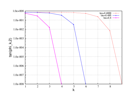
Figure 2: The tangents $\tan\varphi_{k,2}$ from Eq. (34) is plotted for $\tau\in\{0.4,\,0.495,\,0.4999\}$.

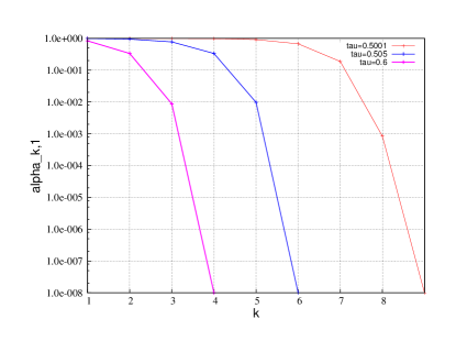
(a) $q_{k,1}$ is plotted for $\tau\in\{0.5001,\,0.505,\,0.6\}$. Here the term $b_{1}$ dominates at every iteration point.

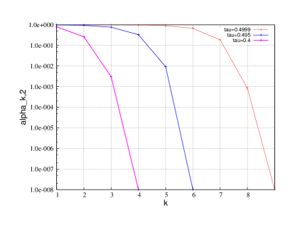
(b) $q_{k,2}$ is plotted for $\tau\in\{0.4999,\,0.495,\,0.4\}$. Here the term $b_{2}$ dominates at every iteration point.

Figure 3: $q_{k,l}$ from Eq. (35) is plotted for $l\in\{1,2\}$ and different values for $\tau$.

4.2 Example 2

Most algorithms in ab initio electronic structure theory compute quantities in terms of one- and two-electron integrals. In [1] we considered the low-rank approximation of the two-electron integrals. In order to demonstrate the convergence of the ALS method on an example of practical interest, we use the order $4$ tensor for the two-electron integrals of the so called AO basis for the CH₄ molecule. We refer the reader to [1] for a detailed description our example. In this example the ALS method converges Q-linearly, see Figure 4.

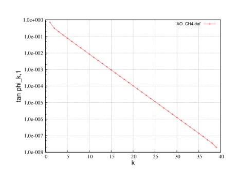
Figure 4: The approximation of two-electron integrals for methane is considered. The tangents of the angle between the current iteration point and the limit point with respect to the iteration number is plotted.

4.3 Example 3

We consider the tensor

$$b_{\lambda}=\bigotimes_{\mu=1}^{3}p+\lambda\left(p\otimes q\otimes q+q\otimes p\otimes q+q\otimes q\otimes p\right)$$

from Ex. 1.3. The vectors $p$ and $q$ are arbitrarily generated orthogonal vectors with norm $1$. The values of $\tan(\varphi_{k}^{1})$ are plotted, where $\varphi_{k}^{1}$ is the angle between $p_{k}^{1}$ and the limit point $p$ (i.e. $\tan\varphi_{k}^{1}=\frac{\left\langle p_{k}^{1},q\right\rangle}{\left\langle p_{k}^{1},p\right\rangle}$, for $k\geq 2$). For the case $\lambda=0.5$ the convergence is sublinearly, whereas for $\lambda=0.2$ it is Q-linearly.

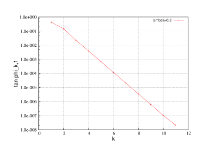
(a) The tangents $\tan\varphi_{k,1}$ for $\lambda=0.2$.

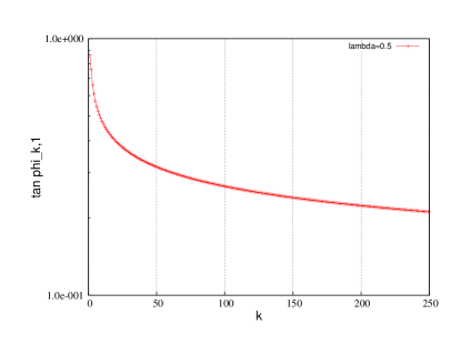
(b) The tangents $\tan\varphi_{k,1}$ for $\lambda=0.5$.

Figure 5: The approximation of $b$ from Example 1.3 is considered. The tangents of the angle between the current iteration point and the limit point with respect to the iteration number is plotted. For $\lambda=1/2$, we have sublinear convergence. But for $\lambda=0.2<1/2$ the sequence converges Q-linearly.

References

- [1] U. Benedikt, A. Auer, M. Espig, and W. Hackbusch. Tensor decomposition in post-hartree–fock methods. i. two-electron integrals and mp2. The Journal of Chemical Physics, 134(5):–, 2011.
- [2] G. Beylkin and M. J. Mohlenkamp. Numerical operator calculus in higher dimensions. Proceedings of the National Academy of Sciences, 99(16):10246–10251, 2002.
- [3] G. Beylkin and M. J. Mohlenkamp. Algorithms for numerical analysis in high dimensions. SIAM Journal on Scientific Computing, 26(6):2133–2159, 2005.
- [4] M. Espig, W. Hackbusch, S. Handschuh, and R. Schneider. Optimization problems in contracted tensor networks. Computing and Visualization in Science, 14(6):271–285, 2011.
- [5] M. Espig, W. Hackbusch, and A. Khachatryan. On the convergence of alternating least squares optimisation in tensor format representations. Preprint, 2014.
- [6] W. Hackbusch. Tensor Spaces and Numerical Tensor Calculus. Springer, 2012.
- [7] S. Holtz, T. Rohwedder, and R. Schneider. The alternating linear scheme for tensor optimization in the tensor train format. SIAM J. Sci. Comput., 34(2):683–713, March 2012.
- [8] T. G. Kolda and B. W. Bader. Tensor decompositions and applications. SIAM REVIEW, 51(3):455–500, 2009.
- [9] M. J. Mohlenkamp. Musings on multilinear fitting. Linear Algebra Appl., 438(2):834–852, 2013.
- [10] J. M. Ortega and W. C. Rheinboldt. Iterative Solution of Nonlinear Equations in Several Variables. Society for Industrial Mathematics, 1970.
- [11] I. V. Oseledets. Dmrg approach to fast linear algebra in the tt-format. Comput. Meth. in Appl. Math., 11(3):382–393, 2011.
- [12] I. V. Oseledets and S. V. Dolgov. Solution of linear systems and matrix inversion in the tt-format. SIAM J. Scientific Computing, 34(5), 2012.
- [13] A. Uschmajew. Local convergence of the alternating least squares algorithm for canonical tensor approximation. SIAM Journal on Matrix Analysis and Applications, 33(2):639–652, 2012.
- [14] André Uschmajew. A new convergence proof for the high-order power method and generalizations. July 2014.
- [15] L. Wang and M. Chu. On the global convergence of the alternating least squares method for rank-one approximation to generic tensors. SIAM Journal on Matrix Analysis and Applications, 35(3):1058–1072, 2014.
- [16] Tong Zhang and Gene H. Golub. Rank-one approximation to high order tensors. SIAM J. Matrix Anal. Appl., 23(2):534–550, February 2001.