Occurrence Rates and Heating Effects of Tangential and Rotational Discontinuities as Obtained from Three-dimensional Simulation of Magnetohydrodynamic Turbulence

Abstract

In solar wind, magnetohydrodynamic (MHD) discontinuities are ubiquitous and often found to be at the origin of turbulence intermittency. They may also play a key role in the turbulence dissipation and heating of the solar wind. The tangential (TD) and rotational (RD) discontinuities are the two most important types of discontinuities. Recently, the connection between turbulence intermittency and proton thermodynamics has been being investigated observationally. Here we present numerical results from three-dimensional MHD simulation with pressure anisotropy and define new methods to identify and to distinguish TDs and RDs. Three statistical results obtained about the relative occurrence rates and heating effects are highlighted: (1) RDs tend to take up the majority of the discontinuities along with time; (2) the thermal states embedding TDs tend to be associated with extreme plasma parameters or instabilities, while RDs do not; (3) TDs have a higher average $T$ as well as perpendicular temperature $T_{\perp}$. The simulation shows that TDs and RDs evolve and contribute to solar wind heating differently. These results will inspire our understanding of the mechanisms that generate discontinuities and cause plasma heating.

1 Introduction

The turbulent solar wind embodies discontinuities (e.g.  Colburn & Sonett, 1966; Tu & Marsch, 1995; Marsch, 2006; Bruno & Carbone, 2013; Paschmann et al., 2013). The tangential discontinuity (TD) and rotational discontinuity (RD) are the two most important yet quite different types: in the deHoffmann-Teller frame, theoretically, TDs have no normal components of $\mathbf{v}$ and $\mathbf{B}$ on both sides, while RDs have normal components, must obey the Walén relation $\mathbf{v}=\pm\mathbf{B}/\sqrt{\mu_{0}\rho}$, and keep $\left|\mathbf{v}\right|$ and $\left|\mathbf{B}\right|$ continuous. Furthermore, TDs allow jumps of density and temperature, while these parameters have the same values on both sides of the RDs. As to the mechanisms of how discontinuities form, there exist two kinds of explanations. There are empirical evidences indicating that discontinuities are boundaries of magnetic flux tubes (Borovsky, 2008; Miao et al., 2011), and there are suppositions that they form locally through nonlinear interactions and may be associated with small random currents (Greco et al., 2009). In Servidio et al. (2011)’s 2D magnetohydrodynamic (MHD) simulation, most discontinuities appear to be TDs. However, in a 3D geometry, it remains unknown which type of discontinuity dominates.

Dissipation of turbulence is considered an important contributor to the heating of the solar wind. Many recent studies concentrated on the role of intermittency and discontinuities in this process. Bale et al. (2009) discovered strongly enhanced fluctuations along the thresholds of plasma instabilities. Osman et al. (2011) reported that high PVI (Partial Variance Increment) levels of various parameters correspond to intensive plasma heating and higher temperatures of electrons as well as ions. Osman et al. (2012) researched a large sample of data from measurements made by the Wind spacecraft and plotted the data distributions in the $(\beta_{\parallel},A)$ parameter plane ($\beta_{\parallel}=p_{\parallel{p}}/(B^{2}/(2\mu_{0}))$, $A=T_{\perp}/T_{\parallel}$). Thus they could show that the distributions are roughly bounded by curves corresponding to the mirror and oblique fire-hose instabilities, that the regions near the instability thresholds have higher averaged PVI, and that events with intense PVIs have $A$ far from unity. Wang et al. (2013) analysed observed discontinuities with the PVI technique and found that the majority of them are RDs, but TDs have more obvious proton temperature increases. These empirical findings inspired us to investigate also the heating effects at the TDs and RDs obtained in our simulation.

Numerical simulations have been employed before to understand plasma heating. Greco et al. (2008) assigned a path through the computational domain and then adopted the notion of PVI to analyse the 3D simulation data sampled along that path. Within their Hall MHD model they thus identified small-scale discontinuities being associated with intermittency. Parashar et al. (2009) demonstrated by use of a 2.5D hybrid model that an ion temperature anisotropy can be created while the protons are heated by magnetic energy dissipation. Karimabadi et al. (2013) conducted a full particle simulation which showed that, triggered by the Kelvin-Helmholtz instability with strong velocity shear, a turbulent cascade generates current sheets heating the plasma locally, and which yielded anisotropic particle distributions in that process. Servidio et al. (2014) allowed for a broader range of $\beta_{\parallel}$ and the strength of the magnetic field fluctuations, thus obtaining results that basically are in accordance with those of Osman et al. (2012). However, neither were the data with high PVIs investigated, nor was the related heating of particles studied. All the mentioned work did also not distinguish between the various types of discontinuities in their simulation data.

Motivated by all these aspects, we will here conduct a 3D numerical simulation with the aim to test new numerical methods to identify and analyse discontinuities, without assuming auxiliary paths along which data are sampled in the simulation domain. Based on this discontinuity identification, we present statistical results in order to investigate the proportion of TDs and RDs in all the discontinuities found, their parameter distribution in the $(\beta_{\parallel},A)$ plane, and the temperature increases in TDs and RDs. Such counts of TDs and RDs and their distributions have, to our knowledge, not been reported previously. These new simulation results will help us to understand better particle heating at intermittent structures in the solar wind, and thus to resolve the turbulence dissipation problem.

In Section 2 we will describe the numerical tools and the methods employed to identify and categorize discontinuities. In Section 3 we present a specific case of a TD and and RD, as well as statistical properties of all discontinuities found in the computation domain. In Section 4 we shall summarize our study, and further discuss relevant physical issues.

2 Methods

2.1 Numerical Model of MHD Turbulence

In order to evaluate the role of temperature anisotropy in MHD turbulence, we adopt the model which employs the compressible ideal MHD equations and incorporates an anisotropic pressure tensor (Meng et al., 2012a, b, 2013):

$$\frac{\partial\rho}{\partial{t}}+\nabla\cdot(\rho\mathbf{v})=0,$$ (1)

$$\frac{\partial\rho\mathbf{v}}{\partial{t}}+\nabla\cdot\left(\rho\mathbf{v}\mathbf{v}+p_{\perp}\mathsf{I}+(p_{\parallel}-p_{\perp})\hat{\mathbf{B}}\hat{\mathbf{B}}-(\mathbf{B}\mathbf{B}-B^{2}\mathsf{I}/2)/\mu_{0}\right)=0,$$ (2)

$$\frac{\partial\mathbf{B}}{\partial{t}}+\nabla\times(-\mathbf{u}\times\mathbf{B})=0,$$ (3)

$$\frac{\partial{p}_{\parallel}}{\partial{t}}+\nabla\cdot(p_{\parallel}\mathbf{u})+2p_{\parallel}\hat{\mathbf{B}}\cdot(\hat{\mathbf{B}}\cdot\nabla)\mathbf{u}=\frac{\delta{p}_{\parallel}}{\delta{t}},$$ (4)

$$\frac{\partial{p}}{\partial{t}}+\nabla\cdot(p\mathbf{u})+2p_{\perp}\nabla\cdot\mathbf{u}/3+2(p_{\parallel}-p_{\perp})\hat{\mathbf{B}}\cdot(\hat{\mathbf{B}}\cdot\nabla)\mathbf{u}/3=0,$$ (5)

where $p=(p_{\parallel}+2p_{\perp})/3$, $\hat{\mathbf{B}}=\mathbf{B}/\left|B\right|$. To describe instabilities correctly, it is common to use a heuristic term of pressure relaxation restricting the temperature anisotropy (Hesse & Birn, 1992; Birn et al., 1995) denoted $\delta{p_{\parallel}}/\delta{t}$. In our numerical simulation we employ this modified MHD model, which is not self-consistent as Vlasov models (e.g. Servidio et al., 2012, 2014). This simplification of our model, on the other hand, will help to understand the role of fluid-like closures of the pressure tensor, which would be dissipative with the pressure-transport terms. Equations 4 and 5 keep the quantities $p_{\perp}/(nB)$ and $B^{2}p_{\parallel}/n^{3}$ adiabatically invariant (Chew et al, 1956), if the RHS of Equation 4 is zero. As Equation 3 is of the ideal MHD type, magnetic helicity is conserved. However, the model still lacks important kinetic physics of the solar wind, e.g. Landau damping and ion cyclotron resonances, which can be vital to turbulence dissipation.

To solve the above system of equations, we utilize the BATSRUS codes (Powell et al., 1999; Tóth et al., 2012). The simulation is conducted in a three-dimensional cartesian coordinate system and encompasses an absolute volume of $(62.8\;\textrm{Mm})^{3}$ that is resolved in $256^{3}$ grid points. The grid resolution ($\sim 250$ km) is well above the ion skin depth ($\sim 100$ km), so Hall-dispersive physics is not included. We use the scheme proposed by Rempel et al. (2009) in order to control numerical diffusion, and by applying such diffusion control strictly keep $\nabla\cdot\mathbf{B}=0$. This method guarantees proper dissipation and correct jump conditions at discontinuities. No explicit diffusive term is included in the numerical simulation code. Yet the magnetic and kinetic energy are subject to decay numerically. This decay can be attributed to the numerical scheme and grid resolution. We apply periodic boundary conditions to all the six surfaces of the simulation box. The initial conditions are set uniformly for $\rho$, $T_{\parallel}$ and $T_{\perp}$, and randomly for $\mathbf{v}$ and $\mathbf{B}$, with the average $\mathbf{v}_{0}=0$ and a finite guide field $\mathbf{B}_{0}\parallel\hat{\mathbf{e}}_{z}$. To simulate the solar wind at 1 AU, the field $\mathbf{B}_{0}$ is chosen as 5 nT, while the Alfvén speed is set at 50 km s^-1, and $p=p_{\parallel}=p_{\perp}$ with $\sqrt{5p/(3\rho)}=50\;\mbox{km}\;\mbox{s}^{-1}$, which corresponds to a proton number density of 5 cm^-3 and an isotropic temperature of $10^{5}\;\mathrm{K}$. For the turbulence part of the fields we take Fourier amplitudes obeying the broadband initial conditions described by Matthaeus et al. (1996), with $\left|\delta\mathbf{B}(\mathbf{k})\right|^{2}=\left|\delta\mathbf{v}(\mathbf{k})\right|^{2}\propto(1+k/k_{\textrm{knee}})^{-q}$ in the range $10^{-7}\;\mathrm{m}^{-1}\leq{k}\leq 8\times 10^{-7}\;\mathrm{m}^{-1}$. The parameter $k_{\textrm{knee}}$ is set to be $3\times 10^{-7}\;\mathrm{m}^{-1}$, and the spectral index $q$ is set so that the slopes of the power spectral densities are both $-5/3$. We take $\sqrt{\left<v^{2}\right>}=30\;\textrm{km s}^{-1}$ (accordingly $\sqrt{\left<\delta{B}^{2}\right>}=3\;\textrm{nT}$). The dimensionless cross-helicity $\sigma=0.9$.

2.2 Methods of Selecting and Categorizing Discontinuities

The analysis of discontinuities calls for reliable methods to select and categorize them in observational or numerical data. To trace abrupt spatial changes of the magnetic field, we use the total variance of increments (TVI) as an indicator and set a threshold for it. To calculate TVI, the total variance is first computed as

$$\left|\Delta{B}\right|=\sqrt{\sum_{\alpha,\beta=x,y,z}(\partial{B}_{\beta}/\partial\alpha)^{2}},$$ (6)

where the partial derivative at grid point $(i,j,k)$ about $x$ is computed as

$$\frac{B_{\bullet}(i+w,j,k)-B_{\bullet}(i-w,j,k)}{2w\delta{x}}.$$ (7)

Here $\delta{x}$ is the grid distance, $B_{\bullet}$ denotes the corresponding component of magnetic field, and $w$ is the width (in this work, we take $w=3$, i.e. within a cuboid of $7^{3}$ grid points). For the $y$ and $z$ derivatives, similar differences along the corresponding directions are used. Then the TVI is the normalized total variance

$$\textrm{TVI}=\left|\Delta{B}\right|/\left<\left|\Delta{B}\right|\right>,$$ (8)

where the angle brackets denote the average over the whole computational domain. This definition is a further development of the previous PVI defined by Greco et al. (2008) (similar to the method adopted before by Marsch & Tu (1994)), which was taken along a given path and hence directionally sensitive. Yet the above TVI includes all directions and thus is unbiased for all points possibly belonging to a discontinuity. The TVI utilises more information from fully 3D data, and accordingly gives more physical insight. However, most solar wind measurements are 1D samples, so the method is inapplicable to such measurements. In the present work, those grid points with $\textrm{TVI}>3$ are actually identifiable as discontinuity points and chosen for subsequent analysis.

At each discontinuity point, we conduct the minimal variance analysis (MVA) (Sonnerup & Cahill, 1967) in its neighbourhood, defined as a cuboid of the same given size for all points considered. Since $B_{n1}=B_{n2}$ is required, the direction of minimal variation can be regarded as the normal of the discontinuity (Sonnerup & Cahill, 1967). In this work, we just consider a discontinuity locally as a small plane that contains the discontinuity point and cuts its neighbouring cuboid into two segments, so that averages of quantities on either side of the plane can be calculated in the segments obtained.

To categorize the discontinuities, we use the criteria defined by Smith (1973), which aim at judging two features: (1) whether $B_{n}=0$ holds, and (2) whether $\left|B\right|$ remains continuous. Hence the parameters $P_{1}=\left|B_{n}\right|/B_{L}$ and $P_{2}=\delta\left|B\right|/B_{L}$ are calculated ($B_{L}$ is the larger of $\left<\left|B\right|\right>$ on both sides). The points with $P_{1}<0.2$ and $P_{2}>0.2$ are categorized as TD, while the ones with $P_{1}>0.4$ and $P_{2}<0.2$ as RD. All the other cases are categorized as ED(either TD or RD type, with $P_{1}<0.4$ and $P_{2}<0.2$) and ND(neither TD nor RD type, with $P_{1}>0.2$ and $P_{2}>0.2$).

The aforementioned analysis only involves magnetic field data. To check and corroborate the results thus obtained, we also analyse the plasma velocity, density, and temperature data. In such case studies, it is trivial to check whether the density or temperature is continuous, but the velocity has to undergo the Walén test for RDs, i.e. one has to test whether $\mathbf{v}-\mathbf{v}_{\textrm{HT}}=\pm\mathbf{b}=\pm\mathbf{B}/\sqrt{\mu_{0}\rho}$, which is usually done statistically in a scatter plot. The Walén test must be conducted in the deHoffmann-Teller frame. To find its velocity $\mathbf{v}_{\textrm{HT}}$, in the cuboid the sum $\sum_{(i,j,k)}\left|(\mathbf{v}_{ijk}-\mathbf{v}_{0})\times\mathbf{B}_{ijk}\right|^{2}$ is to be minimized. The $\mathbf{v}_{0}$ that makes this sum a minimum is then accepted as velocity of the deHoffmann-Teller frame (Sonnerup et al., 1987).

3 Results

The methods described above permit us to select the TDs and RDs from all cases with large TVI, and so we obtain corresponding data sets of discontinuities on which we can do individual and statistical research.

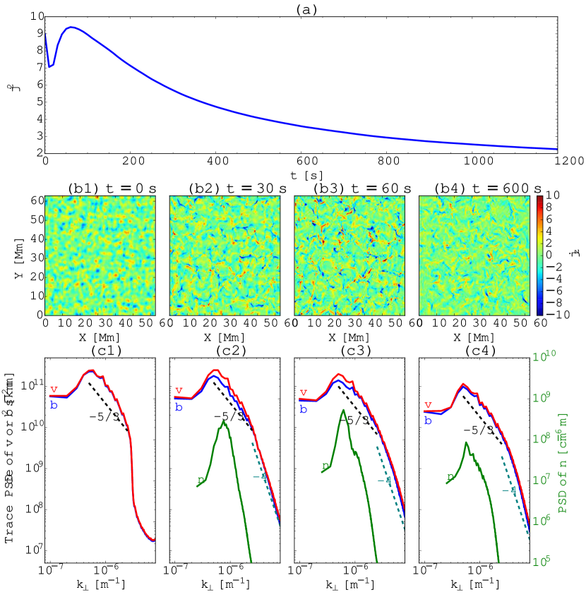
To understand the evolution of the decaying turbulence in our MHD simulation, we plot in Figure 1 the squared current density $\left<j^{2}\right>$ averaged over the whole computational domain. This quantity relates to the curl of the magnetic field and describes its inhomogeneity and energy conversion (dissipation). Its evolution in time clearly shows the following phases: an initial drop, subsequent increase and final decay. This whole trend basically agrees with that found by Matthaeus et al. (1996) in their previous simulation. To further illustrate that process, the $z$-component of current density $j_{z}$ is also plotted in a space-time display. The evolution implies that the initial drop of $\left<j^{2}\right>$ is due to a consumption of the magnetic energy in the compressive turbulent plasma motion, which leads to growing density inhomogeneity. This increase involves the formation of thin and stretched current sheets (see the numerous thin and sharp structures in (b3)). Due to the decay process, the inhomogeneities in (b4) fade away, yet a few current-sheet-like structures remain. The trace power spectral density of $\mathbf{v}$, $\mathbf{b}$, and power spectral density of $n$ are also shown. A region with spectral index close to $-5/3$ seems to be identified.

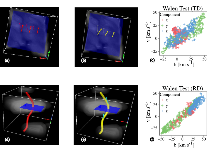
To check our methods and investigate the physical properties of the discontinuities, an individual TD and RD are picked and illustrated in Figure 2. From the TD data we obtain $|B_{n}|/|B|_{L}=0.17$ and $\delta|B|/|B|_{L}=0.45$. The TD has a normal $\hat{\mathbf{n}}=(0.893,-0.355,-0.278)$, almost aligned to the $x$-axis, and an HT velocity $\mathbf{v}_{\mathrm{HT}}=(4.13,-10.96,-41.99)\;\textrm{km~{}s}^{-1}$. In the HT frame, Panels (a) and (b) show that $\mathbf{B}$ and $\mathbf{v}$ across the discontinuity are quasi-parallel to the TD plane. The light grey cloud shows the sub-volume with high TVI and the plane is soaked therein. Panel (c) gives the TD’s Walén test, where the points are rather scattered, but there still exists a correlation of $\mathbf{v}$ and $\mathbf{b}=\mathbf{B}/\sqrt{\mu_{0}\rho}$, especially in the $y$ and $z$ components (the correlation coefficients are $r_{xx},r_{yy},r_{zz}=-0.06,0.88,0.82$). For the RD we find $|B_{n}|/|B|_{L}=0.87$, $\delta|B|/|B|_{L}=0.11$, $\hat{\mathbf{n}}=(0.258,-0.139,0.956)$ and $\mathbf{v}_{\mathrm{HT}}=(1.69,2.17,-55.56)\;\textrm{km s}^{-1}$. Panels (d) and (e) have almost identical and slightly bent stream lines, thus illustrating the confirmation of the Walén relation. Panel (f) shows the correlation coefficients ($r_{xx},r_{yy},r_{zz}=0.87,0.97,0.86$). The temperatures at the respective discontinuity points are also computed. The TD has $T=1.48\times 10^{5}\;\mathrm{K}$, $T_{\parallel}=1.51\times 10^{5}\;\mathrm{K}$, and $T_{\perp}=1.45\times 10^{5}\;\mathrm{K}$, while the RD has $T=1.30\times 10^{5}\;\mathrm{K}$, $T_{\parallel}=1.71\times 10^{5}\;\mathrm{K}$, and $T_{\perp}=1.09\times 10^{5}\;\mathrm{K}$. The TD is by 13.5% hotter than the RD in $T$, and by 33.1% hotter in $T_{\perp}$.

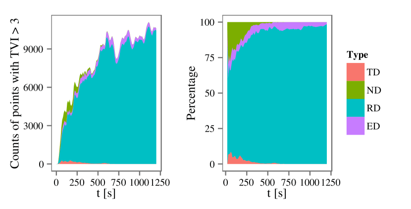
To emphasize furthermore the differences between TDs and RDs, statistical results are presented in Figure 3, where we plot the numbers of discontinuity points of each type as a function of time (left panel), as well as their percentages (right panel). At $t=0$ there are only a few discontinuity points (53 TDs, 25 RDs, 65 EDs, 65 NDs; RDs are even not primary), but then the total number of discontinuity points increases with time, with RD becoming the dominant type. As the temporal evolution progresses, the number of TDs and their percentage first increase yet then decrease again slowly, behaving nearly in phase with that of the changing $\left<j^{2}\right>$, except during its initial drop phase.

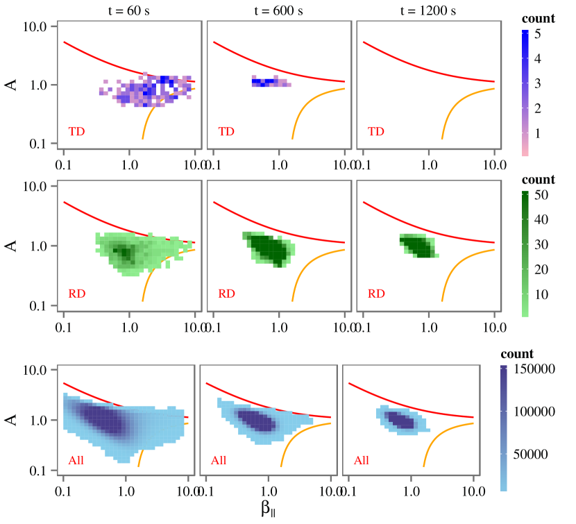
Moreover, in Figure 4 we plot for TDs and RDs their beta and anisotropy locations in the $(\beta_{\parallel},A)$ plane, where darker bins correspond to a higher number of discontinuity points, and with a uniform colour scale to facilitate comparisons for different times. For reference, the threshold curves of the fire-hose and mirror instabilities (Hellinger et al., 2006) are also plotted as orange and red curves, respectively. Apparently, the total numbers of TDs are less than those of RDs. Apart from that, they also distribute differently. At $t=60\;\mathrm{s}$, the TD points tend to aggregate both in the centre region and near to the instability curves. In the decaying phase, the distribution shrinks toward the centre, and disappears finally. The RD points do not show this trend, with their majority still gathering around $\beta_{\parallel}=0.5$, $A=1.0$, i.e. the initial values. At 60 s, some points lie beyond the instability lines but do not congregate there. For reference, the distributions of all grid points are supplied. They resemble those of the RDs.

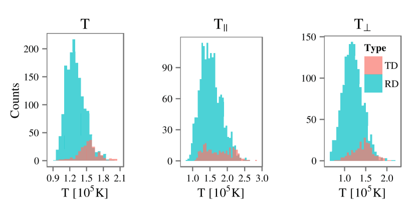
To investigate the heating effect of a discontinuity, the distributions of the temperatures found at the TD and RD points are also provided. Note that simulation of non-adiabatic heating is beyond the scope of this work as no real dissipation is involved. In Figure 5 we plot the distributions of $T$, $T_{\parallel}$ and $T_{\perp}$ at $t=60\;\mathrm{s}$, with the values for TDs in red and RDs in blue. The TDs are slightly hotter in $T$ and $T_{\perp}$. The TDs have $\bar{T}=1.53\times 10^{5}\;\mathrm{K}$ (standard deviation $\sigma=1.84\times 10^{4}\;\mathrm{K}$), whereas the RDs have $\bar{T}=1.30\times 10^{5}\;\mathrm{K}$ ($\sigma=1.68\times 10^{4}\;\mathrm{K}$). Also, TDs have $\bar{T}_{\perp}=1.42\times 10^{5}\;\mathrm{K}$ ($\sigma=2.37\times 10^{4}\;\mathrm{K}$), and RDs have $\bar{T}_{\perp}=1.19\times 10^{5}\;\mathrm{K}$ ($\sigma=2.31\times 10^{4}\;\mathrm{K}$). Since both types of discontinuity evolved in the same plasma with a uniform initial temperature, it is reasonable to conclude that TDs tend to become hotter than RDs, and to infer that TDs may intrinsically be more heated than RDs. The TDs’ increased temperatures may be caused by plasma squeezing and adiabatic compression. In the present case study, the TD has a squeezing (quantified as $\nabla_{n}v_{n}$) whose magnitude is 5.41 times that of the RD.

4 Conclusion

To conclude, in this letter we describe and apply methods to identify and analyse the ubiquitous discontinuities appearing in 3D simulation data, and can therefore present the following statistical results: (1) among the identified discontinuity points, RDs represent the majority, (2) TDs aggregate near the extremes of the fire-hose and mirror instability thresholds, while RDs do not, (3) TDs are hotter than RDs, both in their $T$ and $T_{\perp}$.

However, this work is also limited in some aspects. Though our simulation of decaying turbulence in a closed box can reveal its different stages of evolution in time, the results obtained are difficult to compare with turbulence observations made in the solar wind, where the convected plasma volume is open and can always be filled with fresh waves continuously supplied from a source region. To alleviate this problem (i.e. the difference between the reality and our case study and its temperature distributions), we selected the results obtained at the time when $\left<j^{2}\right>$ is maximal, which may represent a state being close to developed turbulence.

Moreover, MHD though with thermal anisotropy lacks realistic descriptions of microscopic (dissipative) solar wind processes. However, the used MHD model allows us to reduce significantly the computational cost and to investigate discontinuities in three-dimensional space, a virtue of our approach which appears crucial for the analysis. In the identification of discontinuities, we take $w=3$ and the TVI threshold as 3, values which are reasonably chosen but seem somehow arbitrary. Therefore, we also checked the outcome with a different $w$ (ranging from 2 to 5) and TVI threshold (set lower at 2.64) for the statistical study, but found that the results did not change essentially, in terms of identification, normal direction, proportion, and distribution of all discontinuities.

The physical mechanisms generating TDs and RDs should be further investigated. From another aspect, hybrid or full particle simulations should be considered, as they enable the description of kinetic processes in the solar wind as well. Besides, even in 3D MHD simulations, the methods to study large TVI events could be further improved, e.g., possibly by identifying the discontinuities with model structures having a 3D geometric configuration instead of by simply counting their associated points. Such approach may improve the identification of the discontinuities and give better statistics concerning their occurrence rates as well as the percentages of their local temperature increase.

Figure 1: Evolution stages of the decaying turbulence in the MHD simulation. (a): Temporal profile of $\left<j^{2}\right>$ in arbitrary unit. (b): Distribution of the $z$-component of the current density $j_{z}$ in the plane $z=31.4\;\mathrm{Mm}$ at the given times; $j_{z}$ is given in arbitrary unit in agreement with (a). (c): Trace power spectral density of $\mathbf{v}$ (red) and $\mathbf{b}$ (blue), as well as PSD of $n$ (green) at the same times. The horizontal axis represents $k_{\perp}=\sqrt{k_{x}^{2}+k_{y}^{2}}$, while the vertical axis represents $\mathbf{v}$ or $\mathbf{b}$(black, left) and $n$(green, right). Spectral indices $-5/3$(black) and $-4$(cyan) are also plotted in dashed lines for reference.

Figure 2: A TD (top panels) and RD (bottom panels) at $t=60\;\mathrm{s}$. (a) and (b): Schematic of the TD, where the transparent blue plane shows the plane of discontinuity, the red and yellow arrows denote respectively $\mathbf{B}$ and $\mathbf{v}$, the light grey clouds plot the TVI with thicker cloud representing larger values, and the red, blue and green arrows at the box corner indicate the $x$, $y$ and $z$ directions, respectively. The background guide field is along the $z$-direction. (c): Scatter plot of the components of $\mathbf{v}^{\prime}=\mathbf{v}-\mathbf{v}_{\textrm{HT}}$ and $\mathbf{b}=\mathbf{B}/\sqrt{\mu_{0}\rho}$ of the TD. (d) and (e): Schematic of the RD displayed with stream lines; cyan arrows show the direction of the velocity in the HT-frame. (f): Scatter plot for the RD.

Figure 3: Counts (left) of discontinuity points and their proportions (right) for each type. TDs, NDs, RDs and EDs are represented respectively in red, green, cyan and purple.

Figure 4: Temporal evolution of the distributions of TD points (top), RD points (centre), and all grid points in the whole computational region (bottom) in the $(\beta_{\parallel},A=T_{\perp}/T_{\parallel})$ plane, arranged in columns for different times. For reference, the red and orange lines give the thresholds for the mirror and fire-hose instabilities, respectively. The colour of a bin denotes the number of grid points therein.

Figure 5: Distributions of the temperatures associated with the TD and RD points. The left, middle and right sub-plot shows the distribution of $T$, $T_{\parallel}$ and $T_{\perp}$, respectively.

References

- Bale et al. (2009) Bale, S. D., Kasper, J. C., Howes, G. G., et al., 2009, Phys. Rev. Lett., 103, 211101
- Birn et al. (1995) Birn, J., Gary, S. P., & Hesse M. 1995, J. Geophys. Res., 100, 19211
- Borovsky (2008) Borovsky, J. E. 2008, J. Geophys. Res., 113, A08110
- Bruno & Carbone (2013) Bruno, R., & Carbone, V., “The Solar Wind as a Turbulence Laboratory”, LRSP, 10, 2. URL(cited on 15 Dec 2014): http://solarphysics.livingreviews.org/Articles/lrsp-2013-2/
- Chew et al (1956) Chew, G.F., Goldberger, M.L., & Low, F.E. 1956, RSPSA, 236, 112
- Clyne et al (2007) Clyne, J., Mininni, P., Norton, A., & Rast, M. 2007, NJPh, 9, 301
- Colburn & Sonett (1966) Colburn, D. S., & Sonett, C. P. 1966, Space Sci. Rev., 5, 439
- Goldstein et al. (1995) Goldstein, M., Roberts, D., & Matthaeus, W. 1995, ARA&A, 33, 283
- Greco et al. (2008) Greco, A., Chuychai, P., Matthaeus, W. H., Servidio, S., & Dmitruk, P. 2008, Geophys. Res. Lett., 35, L19111
- Greco et al. (2009) Greco, A., Matthaeus, W. H., Servidio, S., Chuychai, P., & Dmitruk, P. 2009, ApJ, 691, L111
- Hellinger et al. (2006) Hellinger, P., Trávníček, P., Kasper, J. C., & Lazarus, A. J. 2006, Geophys. Res. Lett., 33, L09101
- Hesse & Birn (1992) Hesse, M., & Birn, J. 1992, J. Geophys. Res., 97, 10643
- Karimabadi et al. (2013) Karimabadi, H., Roytershteyn, V., Wan, M. et al., 2013, PhPl, 20, 012303
- MacBride et al. (2008) MacBride, B., Smith, C., & Forman, M. 2008, ApJ, 679, 1644
- Marsch & Tu (1994) Marsch, E., & Tu, C. Y. 1994, AnGeo, 12, 1127
- Marsch (2006) Marsch, E., “Kinetic Physics of the Solar Wind”, LRSP, 3, 1. URL(cited on 14 Dec 2014): http://solarphysics.livingreviews.org/Articles/lrsp-2006-1/
- Matthaeus et al. (1996) Matthaeus, W. H., Ghosh, S., Oughton, S., & Roberts, D. A. 1996, J. Geophys. Res., 101, 7619
- Meng et al. (2012a) Meng, X., Tóth, G., Liemohn, M. W., Gombosi, T. I., & Runov, A. 2012, J. Geophys. Res., 117, A08216
- Meng et al. (2012b) Meng, X., Tóth, G., Sokolov, I. V., & Gombosi, T. I. 2012, JCoPh, 231, 3610
- Meng et al. (2013) Meng, X., Tóth, G., Glocer, A., Fok, M. C., & Gombosi, T. I. 2013, J. Geophys. Res., 118, 5639
- Miao et al. (2011) Miao, B., Peng, B., & Li, G. 2011, AnGeo, 29, 237
- Osman et al. (2011) Osman, K. T., Matthaeus, W. H., Greco, A., & Servidio, S. 2011, ApJ, 727, L11
- Osman et al. (2012) Osman, K. T., Matthaeus, W. H., Hnat, B., & Chapman, S. C. 2012, Phys. Rev. Lett., 108, 261103
- Parashar et al. (2009) Parashar, T. N., Shay, M. A., Cassak, P. A., & Matthaeus, W. H. 2009, PhPl, 16, 032310
- Paschmann et al. (2013) Paschmann, G., Halland, S., Sonnerup, B., & Knetter, T. 2013, AnGeo, 31, 871
- Powell et al. (1999) Powell, K. G., Roe, P. L., Linde, T. J., Gombosi, T. I., & De Zeeuw, D. L. 1999, JCoPh, 154, 284
- Rempel et al. (2009) Rempel, M., Schüssler, M., & Knölker, M. 2009, ApJ, 691, 640
- Servidio et al. (2011) Servidio, S., Dmitruk, P., Greco, A. et al., 2011, NPGeo, 18, 675
- Servidio et al. (2012) Servidio, S., Valentini, F., Califano, F. & Veltri, P. 2012, Phys. Rev. Lett., 108, 045001
- Servidio et al. (2014) Servidio, S., Osman, K. T., Valentini, F. et al., 2014, ApJ, 781, L27
- Smith (1973) Smith, E. J. 1973, J. Geophys. Res., 78, 2054
- Sonnerup & Cahill (1967) Sonnerup, B. U. Ö. & Cahill, L. J. Jr. 1967, J. Geophys. Res., 72, 171
- Sonnerup et al. (1987) Sonnerup, B. U. Ö., Papamastorakis, I., Paschmann, G., & Lühr, H. 1987, J. Geophys. Res., 92, 12137
- Tóth et al. (2012) Tóth, G., van der Holst, B., Sokolov, I. V., et al., 2012, JCoPh, 231, 870
- Tu & Marsch (1995) Tu, C. Y., & Marsch, E. 1995, Space Sci. Rev., 73, 1
- Wang et al. (2013) Wang, X., Tu, C. Y., He, J. S., Marsch, E., & Wang, L. H. 2013, ApJ, 772, L14