Standard Model evaluation of $\varepsilon_{K}$ using lattice QCD inputs for $\hat{B}_{K}$ and $V_{cb}$

Abstract

We report the Standard Model evaluation of the indirect CP violation parameter $\varepsilon_{K}$ using inputs determined from lattice QCD: the kaon bag parameter $\hat{B}_{K}$, $\xi_{0}$, $|V_{us}|$ from the $K_{\ell 3}$ and $K_{\mu 2}$ decays, and $|V_{cb}|$ from the axial current form factor for the exclusive decay $\bar{B}\to D^{*}\ell\bar{\nu}$ at zero-recoil. The theoretical expression for $\varepsilon_{K}$ is thoroughly reviewed to give an estimate of the size of the neglected corrections, including long distance effects. The Wolfenstein parametrization $(|V_{cb}|,\lambda,\bar{\rho},\bar{\eta})$ is adopted for CKM matrix elements which enter through the short distance contribution of the box diagrams. For the central value, we take the Unitarity Triangle apex $(\bar{\rho},\bar{\eta})$ from the angle-only fit of the UTfit collaboration and use $V_{us}$ as an independent input to fix $\lambda$. We find that the Standard Model prediction of $\varepsilon_{K}$ with exclusive $V_{cb}$ (lattice QCD results) is lower than the experimental value by $3.4\sigma$. However, with inclusive $V_{cb}$ (results of the heavy quark expansion), there is no gap between the Standard Model prediction of $\varepsilon_{K}$ and its experimental value. For the calculation of $\varepsilon_{K}$, we perform the renormalization group running to obtain $\eta_{cc}$ at next-to-next-to-leading-order; we find $\eta_{cc}^{\mathrm{NNLO}}=1.72(27)$.

I Introduction

CP violation in nature was first discovered in an experiment with the neutral kaon system in 1964 Christenson et al. (1964). There are two kinds of CP violation in the neutral kaon system: one is the indirect CP violation due to CP-asymmetric impurity in the kaon eigenstates in nature, and the other is the direct CP violation due to the CP violating nature of the weak interaction Alavi-Harati et al. (1999); Fanti et al. (1999). CP violating observables are prime candidates in searches for physics beyond the Standard Model. Experimentally, CP violation in the neutral kaon system is known more precisely than in any other physical system. Here, we focus on the indirect CP violation in neutral kaons.

Indirect CP violation in the neutral kaon system is parametrized by $\varepsilon_{K}$

$$\varepsilon_{K}\equiv\frac{\mathcal{A}(K_{L}\to\pi\pi(I=0))}{\mathcal{A}(K_{S}\to\pi\pi(I=0))}\,,$$ (1)

where $K_{L}$ and $K_{S}$ are the neutral kaon states in nature, and $I=0$ represents the isospin of the final two-pion state. In experiment Olive et al. (2014),

$$\varepsilon_{K} =(2.228\pm 0.011)\times 10^{-3}\times e^{i\phi_{\varepsilon}}\,,$$

$$\phi_{\varepsilon} =43.52\pm 0.05{}^{\circ}\,.$$ (2)

Here, the $\varepsilon_{K}$ value represents an $\approx 0.2\%$ impurity of the CP even eigenstate in the $K_{L}$ state, which contains 99.8% of the CP odd eigenstate.

We can also calculate $\varepsilon_{K}$ directly from the Standard Model (SM). In the SM, CP violation comes solely from a single phase in the CKM matrix elements Kobayashi and Maskawa (1973); Cabibbo (1963). The SM allows the mixing of neutral kaons $K^{0}(d\bar{s})$ and $\overline{K}^{0}(s\bar{d})$ through loop processes, and describes contributions to the mass splitting $\Delta M_{K}$ and $\varepsilon_{K}$. Hence, we can test the SM through CP violation by comparing the experimental and theoretical values of $\varepsilon_{K}$.

In the SM, the master formula for $\varepsilon_{K}$ is

$$\varepsilon_{K}= e^{i\theta}\sqrt{2}\sin{\theta}\Big{(}C_{\varepsilon}\hat{B}_{K}X_{\text{SD}}+\frac{\xi_{0}}{\sqrt{2}}+\xi_{\text{LD}}\Big{)}$$

$$+\mathcal{O}(\omega\varepsilon^{\prime})+\mathcal{O}(\xi_{0}\Gamma_{2}/\Gamma_{1})\,,$$ (3)

where $C_{\varepsilon}$ is a well-known coupling given in Eq. (68), and $X_{\text{SD}}$ is the short distance contribution from the box diagrams given in Eq. (II.3). Here, the major contribution to $\varepsilon_{K}$ comes from the $\hat{B}_{K}$ term, and the minor contribution of about 5% comes from the $\xi_{0}$ term. The remaining contribution of $\xi_{\text{LD}}$ is about 2% coming from the long distance effect on $\varepsilon_{K}$ Christ et al. (2013, 2014). In Section II, we re-derive the leading contribution given in Refs. Buras and Guadagnoli (2008); Buras et al. (2010); Donoghue et al. (1992). We also explicitly derive higher order corrections, including the long distance contribution, in this paper. A similar formula without the long distance correction $\xi_{\text{LD}}$ and higher order terms appears in Refs. Buras and Guadagnoli (2008); Buras et al. (2010).

In order to calculate $\varepsilon_{K}$ directly from the SM, we use input parameters obtained from lattice QCD and experiments. In particular, $\hat{B}_{K}$ and $V_{cb}$ have dominated the statistical and systematic uncertainty in the SM evaluation of $\varepsilon_{K}$ for a long time.

During the past decade, lattice QCD has made significant progress in calculating $\hat{B}_{K}$ so that its error is reduced dramatically, down to the $\approx 1.3\%$ level at present. This result is available from the Flavour Lattice Averaging Group (FLAG) Aoki et al. (2013). It is obtained by taking an average of the $\hat{B}_{K}$ results from a number of lattice QCD groups Bae et al. (2014a); Arthur et al. (2013); Laiho and Van de Water (2011); Bae et al. (2012); Durr et al. (2011). We calculate $\varepsilon_{K}$ using two different input values of $\hat{B}_{K}$: one is the FLAG result Aoki et al. (2013), and the other is the most updated result from the SWME collaboration Bae et al. (2014b).

It is also noteworthy that the lattice calculation of the amplitude $\mathrm{Im}A_{2}$ related to the decay $K\to\pi\pi(I=2)$ Blum et al. (2012) makes it possible to determine $\xi_{0}$ more precisely.

Another important input parameter to $\varepsilon_{K}$ is $V_{cb}$. There are two independent methods to determine $V_{cb}$: one is the exclusive method Bailey et al. (2014a), and the other is the inclusive method Gambino and Schwanda (2014); Alberti et al. (2015). In the exclusive method Bailey et al. (2014a), one uses lattice QCD to calculate semileptonic form factors for the decays $\bar{B}\to D^{(*)}\ell\bar{\nu}$. In the inclusive method Gambino and Schwanda (2014); Alberti et al. (2015), one performs analysis on $B\to X_{c}\ell\bar{\nu}$ decay processes using the heavy quark expansion Uraltsev (2000). Here, we use both the exclusive and inclusive $V_{cb}$ to determine $\varepsilon_{K}$, and we compare the results with each other and experiment.

We use the Wolfenstein parametrization for the CKM matrix Buchalla et al. (1996), truncating the series at $\mathcal{O}(\lambda^{7})\approx 10^{-5}$. Here, we use three different choices of Wolfenstein parameters: (1) $\lambda$, $\bar{\rho}$, and $\bar{\eta}$ from the global fit of the CKMfitter collaboration Charles et al. (2005); Hocker et al. (2001), (2) $\lambda$, $\bar{\rho}$, and $\bar{\eta}$ from the global fit of the UTfit collaboration Bona et al. (2005, 2008), and (3) $\bar{\rho}$ and $\bar{\eta}$ from an angle-only fit (AOF) from the UTfit collaboration Bevan et al. (2013), with an independent input for $\lambda$ directly from $V_{us}$ Olive et al. (2014). In all the cases, we take $V_{cb}$ instead of the Wolfenstein parameter $A$ from the unitarity triangle (UT) analysis. We emphasize that the AOF does not use $\varepsilon_{K}$, $\hat{B}_{K}$, and $V_{cb}$ to determine the UT apex $\bar{\rho}$ and $\bar{\eta}$. Hence, it provides a self-consistent way to test the validity of the SM with $\varepsilon_{K}$, using the lattice results for $\hat{B}_{K}$ and $V_{cb}$ with no correlation between $(\hat{B}_{K},V_{cb})$ and $(\bar{\rho},\bar{\eta})$.

To estimate the effect of correlations in lattice input parameters, we note that $V_{cb}$ dominates the error in $\varepsilon_{K}$, and the FLAG $\hat{B}_{K}$ Aoki et al. (2013) is dominated by the BMW collaboration result Durr et al. (2011). We assume that there is no correlation between the BMW $\hat{B}_{K}$ and the exclusive $V_{cb}$ from the FNAL/MILC form factor Bailey et al. (2014a), because their gauge ensembles are independent. Hence, we assume that the correlation between the FLAG $\hat{B}_{K}$ and the FNAL/MILC $V_{cb}$ are negligibly small. However, when we use the SWME $\hat{B}_{K}$ Bae et al. (2014b), there must be an inevitable correlation with the FNAL/MILC result for exclusive $V_{cb}$. In this case, we consider $+50\%$ correlation and $-50\%$ anti-correlation between the SWME $\hat{B}_{K}$ and the exclusive $V_{cb}$ to estimate the systematic error due to the correlation between them. The RBC/UKQCD collaboration calculated $\xi_{0}$ using domain-wall fermions, which is also completely independent. Hence, we assume that $\xi_{0}$ is uncorrelated with the other lattice inputs $\hat{B}_{K}$ and $V_{cb}$.

When we determine the value of $\varepsilon_{K}$, we take into account the correlation between the SWME $\hat{B}_{K}$ and the FNAL/MILC $V_{cb}$ and assume that the other input parameters are uncorrelated. We use the Monte Carlo method to calculate the $\varepsilon_{K}$ distribution from the SM. The results are cross-checked using the standard error propagation method.

In Section II, we review neutral kaon mixing and derive the master formula for $\varepsilon_{K}$ from the SM. Here, we give an estimate for the size of truncated small corrections. In Section III, we explain each input parameter in detail. Here, we also explain details on how we populate input distributions using the Monte Carlo method and how we determine errors on $\varepsilon_{K}$ considering different input combinations and correlations among them. In Section IV, we present the results for $\varepsilon_{K}$ obtained using various combinations of input parameters. In Section V, we conclude.

II Review of $\varepsilon_{K}$

II.1 Effective Hamiltonian

Let us first review the theoretical formalism of neutral kaon mixing in the SM Buras (1998). Let us consider a state that is initially (at $t=0$) a superposition of $K^{0}(d\bar{s})$ and $\overline{K}^{0}(s\bar{d})$:

$$|\psi(0)\rangle =a(0)|K^{0}\rangle+b(0)|\overline{K}^{0}\rangle\,.$$ (4)

This state will evolve in time, and part of it will decay into final states $\{f_{1},f_{2},\ldots\}$ as follows.

$$|\psi(t)\rangle =a(t)|K^{0}\rangle+b(t)|\overline{K}^{0}\rangle$$

$$\hskip 24.0pt+c_{1}(t)|f_{1}\rangle+c_{2}(t)|f_{2}\rangle+\cdots\,.$$ (5)

If we are interested in calculating only the values of $a(t)$ and $b(t)$, but not the values of $c_{i}(t)$, and if the time $t$ is much larger than the typical strong interaction scale, then we can use the simplified formalism in Ref. Weisskopf and Wigner (1930a, b). In this formalism, the time evolution is described by a $2\times 2$ effective Hamiltonian $H_{\text{eff}}$ that is not Hermitian, which allows the neutral kaons to oscillate and to decay.

The neutral kaon system forms a two dimensional subspace of the Hilbert space of the total Hamiltonian $H=H_{\text{0}}+H_{\text{w}}$. $H_{\text{0}}$ is the strong interaction Hamiltonian which defines the full Hilbert space. Decays into different strong eigenstates are mediated by the weak interaction Hamiltonian $H_{\text{w}}$, which is treated as a perturbation.

In the 2-dimensional subspace, the time evolution of the neutral kaon state vector can be described by the effective Hamiltonian $H_{\text{eff}}$,

$$i\frac{d}{dt}\lvert K(t)\rangle =H_{\text{eff}}\lvert K(t)\rangle\,.$$ (6)

The effective Hamiltonian consists of two Hermitian operators $M$ and $\Gamma$,

$$H_{\text{eff}}=M-i\frac{\Gamma}{2}\,.$$ (7)

The dispersive part $M$ defines masses of the neutral kaon states, which correspond to the kaon eigenstates in nature, and the absorptive part $\Gamma$ defines decay widths of the mass eigenstates in the presence of the weak interaction $H_{\text{w}}$. The effective Hamiltonian itself, however, is not Hermitian. It is a necessary consequence to take into account kaon decay amplitudes that have final strong eigenstates which do not belong to the neutral kaon subspace, as one can see in Eq. (5).

The decay processes can be systematically described by the perturbative corrections to the effective Hamiltonian of the subspace Wang and Sanda (1997). In the second order in $H_{\text{w}}$, or equivalently second order in the Fermi coupling constant $G_{F}$, the results are, as shown by the famous Wigner-Weisskopf formula Weisskopf and Wigner (1930a, b),

$$M_{\alpha\beta}= m_{0}\delta_{\alpha\beta}+\langle\alpha\lvert H_{\text{w}}\rvert\beta\rangle$$

$$-\mathcal{P}\sum_{C}\frac{\langle\alpha\lvert H_{\text{w}}\rvert C\rangle\langle C\lvert H_{\text{w}}\rvert\beta\rangle}{E_{C}-m_{K^{0}}}\,,$$ (8)

$$\Gamma_{\alpha\beta}= 2\pi\sum_{C}\langle\alpha\lvert H_{\text{w}}\rvert C\rangle\langle C\lvert H_{\text{w}}\rvert\beta\rangle\delta(E_{C}-m_{0})\,,$$ (9)

where $m_{K^{0}}$ is the mass of the neutral kaons $K^{0}$ and $\overline{K}^{0}$, $\mathcal{P}$ denotes the principal value, $\lvert C\rangle$ is an intermediate state with energy $E_{C}$ which belongs to the full Hilbert space, and the summation over $C$ includes integration over the continuous quantum numbers. Here, we ignore a tiny experimental mass difference between $K^{0}$ and $\overline{K}^{0}$, since we assume CPT invariance throughout this paper. Hence, the masses of a particle and its anti-particle are the same.

The leading correction to the off-diagonal components of $M_{\alpha\beta}$ comes from the four-quark $\Delta S=2$ operator of dimension 6. It is built from a product of two weak current-current interactions by integrating out $W$-bosons and heavy quarks in the box loop diagrams. This is a short distance contribution, and it is the leading effect which is responsible for the indirect CP violation in neutral kaon mixing. This short distance effect is explained in Section II.3 in detail. If there exists a fundamental $\Delta S=2$ interaction, the so-called superweak interaction $H_{\text{sw}}$, which is absent in the SM, it also contributes to the off-diagonal components $M_{\alpha\beta}$ Winstein and Wolfenstein (1993). Neutral kaons could decay into an intermediate state $\lvert C\rangle$ as a result of $\Delta S=1$ transitions. The parts which involve these intermediate states $\lvert C\rangle$ in Eq. (II.1) and Eq. (9) constitute the long distance contributions.

The time independence of the effective Hamiltonian is a consequence of the Wigner-Weisskopf approximation, which takes the interaction time to infinity and turns the interaction adiabatically off Wang and Sanda (1997); Pokorski (2000). The well-known exponential decay law follows from this approximation. So a deviation from the conventional exponential decay gives an estimate of the accuracy of the Wigner-Weisskopf approximation. These corrections to the exponential decay, with present and foreseeable experimental precision Wang and Sanda (1997); Liang and Wang (2001), are far beyond the precision that we pursue here for the value of $\varepsilon_{K}$ in the SM. Hence, we neglect these corrections in this paper.

Before considering explicit calculation of the matrix elements on the right hand side of Eq. (II.1) and Eq. (9), we focus on their parametrization. From the Hermiticity of $M$ and $\Gamma$, each of them is parametrized with 4 real variables

$$M= \begin{pmatrix}M_{1}&im^{\prime}+\delta_{m^{\prime}}\\ -im^{\prime}+\delta_{m^{\prime}}&M_{2}\end{pmatrix}\,,$$ (10)

$$\Gamma= \begin{pmatrix}\Gamma_{1}&i\gamma^{\prime}+\delta_{\gamma^{\prime}}\\ -i\gamma^{\prime}+\delta_{\gamma^{\prime}}&\Gamma_{2}\end{pmatrix}\,.$$ (11)

Further simplification

$$\delta_{m^{\prime}}=0\,,\quad\delta_{\gamma^{\prime}}=0$$ (12)

follows from CPT invariance, $(CPT)O(CPT)^{-1}=O$, where $O=M,\Gamma$, and with a specific basis made of the CP eigenstates: $\{\lvert K_{1}\rangle,\lvert K_{2}\rangle\}$ Winstein and Wolfenstein (1993).

Assuming the strong interaction has CP symmetry, the neutral kaon subspace can be spanned by the CP even $\lvert K_{1}\rangle$ and odd $\lvert K_{2}\rangle$ eigenstates

$$|K_{1}\rangle= \frac{1}{\sqrt{2}}\big{(}\lvert K^{0}\rangle-\lvert\overline{K}^{0}\rangle\big{)}\,,$$

$$|K_{2}\rangle= \frac{1}{\sqrt{2}}\big{(}\lvert K^{0}\rangle+\lvert\overline{K}^{0}\rangle\big{)}\,.$$ (13)

We adopt a phase convention Buras (1998)

$$CP\lvert K^{0}\rangle=-\lvert\overline{K}^{0}\rangle\,,$$ (14)

and for time reversal $T$

$$T\lvert K^{0}\rangle=-\lvert K^{0}\rangle\,,\quad T\lvert\overline{K}^{0}\rangle=-\lvert\overline{K}^{0}\rangle\,.$$ (15)

Here, note that the incoming state becomes an outgoing state under time reversal and vice versa. Then

$$\lvert\overline{K}_{1}\rangle= CPT\lvert K_{1}\rangle=-\lvert K_{1}\rangle\,,$$

$$\lvert\overline{K}_{2}\rangle= CPT\lvert K_{2}\rangle=\lvert K_{2}\rangle\,.$$ (16)

Then we can verify the constraints in Eq. (12),

$$\langle K_{1}\lvert M\rvert K_{2}\rangle= \langle\overline{K}_{2}\lvert(CPT)M^{\dagger}(CPT)^{-1}\rvert\overline{K}_{1}\rangle$$

$$= -\langle K_{2}\lvert M\rvert K_{1}\rangle\,.$$ (17)

The same relation also holds for $\Gamma$. Here, the Hermitian conjugate arises from the anti-unitarity of the time reversal symmetry.

II.2 $\varepsilon_{K}$ and $\tilde{\varepsilon}$

The physical states $K_{S}$ and $K_{L}$ are approximately CP even and odd, respectively. In other words, the physical eigenstates of the effective Hamiltonian $H_{\text{eff}}$ in Eq. (7) include a tiny impurity ($\approx 10^{-3}$) of the opposite CP eigenstate defined in Eq. (II.1). The physical eigenstates can be written with small mixing parameters $\tilde{\varepsilon}_{S}$ and $\tilde{\varepsilon}_{L}$,

$$\lvert K_{S}\rangle= \frac{1}{\sqrt{1+\lvert\tilde{\varepsilon}_{S}\rvert^{2}}}(\lvert K_{1}\rangle+\tilde{\varepsilon}_{S}\lvert K_{2}\rangle)\,,$$

$$\lvert K_{L}\rangle= \frac{1}{\sqrt{1+\lvert\tilde{\varepsilon}_{L}\rvert^{2}}}(\lvert K_{2}\rangle+\tilde{\varepsilon}_{L}\lvert K_{1}\rangle)\,.$$ (18)

Their eigenvalues are

$$\lambda_{S}=\bar{\lambda}-\Delta\lambda\,,\;\lambda_{L}=\bar{\lambda}+\Delta\lambda\,,$$ (19)

where

$$\bar{\lambda}=\frac{1}{2}\left\{(M_{1}+M_{2})-\frac{i}{2}(\Gamma_{1}+\Gamma_{2})\right\}\,,$$ (20)

$$\Delta\lambda=\frac{1}{2}\sqrt{\Big{(}\Delta M+\frac{i}{2}\Delta\Gamma\Big{)}^{2}+4\Big{(}m^{\prime}-\frac{i}{2}\gamma^{\prime}\Big{)}^{2}}\,,$$ (21)

and

$$\Delta M=M_{2}-M_{1}\,,\;\Delta\Gamma=\Gamma_{1}-\Gamma_{2}\,.$$ (22)

Eliminating the eigenvalues $\lambda_{S,L}$ from the system of eigenvalue equations

$$\Big{(}M_{1}-\frac{i}{2}\Gamma_{1}-\lambda_{S}\Big{)}+\tilde{\varepsilon}_{S}\Big{(}im^{\prime}+\frac{1}{2}\gamma^{\prime}\Big{)} =0\,,$$

$$\tilde{\varepsilon}_{S}\Big{(}M_{2}-\frac{i}{2}\Gamma_{2}-\lambda_{S}\Big{)}-\Big{(}im^{\prime}+\frac{1}{2}\gamma^{\prime}\Big{)} =0\,,$$

$$\Big{(}M_{2}-\frac{i}{2}\Gamma_{2}-\lambda_{L}\Big{)}-\tilde{\varepsilon}_{L}\Big{(}im^{\prime}+\frac{1}{2}\gamma^{\prime}\Big{)} =0\,,$$

$$\tilde{\varepsilon}_{L}\Big{(}M_{1}-\frac{i}{2}\Gamma_{1}-\lambda_{L}\Big{)}+\Big{(}im^{\prime}+\frac{1}{2}\gamma^{\prime}\Big{)} =0$$ (23)

leads to the condition

$$(\tilde{\varepsilon}_{S,L}^{2}+1)\Big{(}im^{\prime}+\frac{1}{2}\gamma^{\prime}\Big{)}-\tilde{\varepsilon}_{S,L}\Big{(}\Delta M+\frac{i}{2}\Delta\Gamma\Big{)}=0$$ (24)

that the mixing parameters have to satisfy. The quadratic equation in Eq. (24) has two solutions. One of them is very small ($\approx 10^{-3}$) and the other is very large ($\approx 10^{+3}$). Hence, it is obvious that the two mixing parameters are equal, since we assume that the mixing impurity is in the level of $\approx 10^{-3}$. Hence, we will use the mixing parameter $\tilde{\varepsilon}$

$$\tilde{\varepsilon}\equiv\tilde{\varepsilon}_{S}=\tilde{\varepsilon}_{L}\,.$$ (25)

Since we know that $\mathcal{\lvert\tilde{\varepsilon}\rvert}\approx 10^{-3}$, we can rewrite Eq. (24) as follows,

$$\tilde{\varepsilon}=\tilde{\varepsilon}_{(0)}(1+\tilde{\varepsilon}^{2})\,,$$ (26)

where

$$\tilde{\varepsilon}_{(0)}\equiv\frac{i\Big{(}m^{\prime}-\frac{i}{2}\gamma^{\prime}\Big{)}}{\Delta M+\frac{i}{2}\Delta\Gamma}\,.$$ (27)

Then, Eq. (26) can be solved iteratively near the leading order solution $\tilde{\varepsilon}_{(0)}$,

$$\tilde{\varepsilon}=\tilde{\varepsilon}_{(0)}+\tilde{\varepsilon}_{(0)}^{3}+2\tilde{\varepsilon}_{(0)}^{5}+5\tilde{\varepsilon}_{(0)}^{7}+\cdots\,.$$ (28)

To complete the connection between $\tilde{\varepsilon}$ and $\varepsilon_{K}$, we need to consider kaon decay amplitudes Cirigliano et al. (2012). Define the isospin amplitude $A_{I}$ and phases $\xi_{I}$ and $\delta_{I}$ by

$$\mathcal{A}(K^{0}\to\pi\pi(I)) \equiv A_{I}e^{i\delta_{I}}=\lvert A_{I}\rvert e^{i\xi_{I}}e^{i\delta_{I}}\,.$$ (29)

Then, in our phase convention, which is one of the most popular conventions Branco et al. (1999),

$$\mathcal{A}(\overline{K}^{0}\to\pi\pi(I))= -A^{\ast}_{I}e^{i\delta_{I}}=-\lvert A_{I}\rvert e^{-i\xi_{I}}e^{i\delta_{I}}\,,$$ (30)

and

$$\mathcal{A}(K_{1}\to\pi\pi(I)) =\sqrt{2}\mathrm{Re}A_{I}e^{i\delta_{I}}\,,$$

$$\mathcal{A}(K_{2}\to\pi\pi(I)) =i\sqrt{2}\mathrm{Im}A_{I}e^{i\delta_{I}}\,,$$ (31)

where the phase $\delta_{I}$ is equal to the $S$-wave scattering phase shift of the final two-pion state by the strong interaction, and the subscript $I$ represents the isospin of the final state. Assuming isospin symmetry, this comes from Watson’s theorem Donoghue et al. (1992); Cirigliano et al. (2012). Watson’s theorem is based on time reversal symmetry implicitly. Because the final state scattering only involves $H_{0}$, application of Watson’s theorem concerns the time reversal symmetry of the strong interaction. It is equivalent to the CP symmetry, if we assume CPT invariance. Here, note that $\xi_{I}$ represents the effect of the violation of Watson’s theorem.

If the weak Hamiltonian $H_{\text{w}}$ respected CP symmetry, which is equivalent to time reversal symmetry under CPT invariance, then Watson’s theorem must hold to guarantee that $A_{I}$ must be real in this case Donoghue et al. (1992). However, we know that $H_{\text{w}}$ breaks CP symmetry through the existence of a single phase in the CKM matrix, and so it also violates time reversal symmetry. As a consequence, Watson’s theorem is violated, and so $A_{I}$ becomes complex, which generates the phase $\xi_{I}\neq 0$, in general. Hence, the weak phases $\xi_{I}$ parametrize the direct CP violation in the weak interaction with a non-zero phase difference, $\mathrm{Im}(A_{2}/A_{0})$, which is independent of phase convention Buras (1998).

Now, let us focus on $\gamma^{\prime}$ and $\Delta\Gamma$ in Eq. (27). We will address $m^{\prime}$ and $\Delta M$ later in Section II.3 and Section II.4. Let us divide both numerator and denominator of Eq. (27) by $\Delta M$; we obtain

$$\tilde{\epsilon}_{(0)} =e^{i\theta}\sin{\theta}\Big{(}\frac{m^{\prime}}{\Delta M}-i\cot{\theta}\frac{\gamma^{\prime}}{\Delta\Gamma}\Big{)}$$

$$=e^{i\theta}\sin{\theta}\Big{(}\frac{m^{\prime}}{\Delta M}-i\xi_{0}\cot{\theta}\Big{)}+\mathcal{O}(\omega\varepsilon^{\prime})$$

$$\hskip 24.0pt+\mathcal{O}(\xi_{0}\Gamma_{2}/\Gamma_{1})\,,$$ (32)

where

$$\tan{\theta} \equiv\frac{2\Delta M}{\Delta\Gamma}\,,$$ (33)

$$\varepsilon^{\prime} \equiv e^{i(\delta_{2}-\delta_{0})}\frac{i\omega}{\sqrt{2}}\left(\frac{\mathrm{Im}{A_{2}}}{\mathrm{Re}{A_{2}}}-\frac{\mathrm{Im}{A_{0}}}{\mathrm{Re}{A_{0}}}\right)$$

$$=e^{i(\delta_{2}-\delta_{0})}\frac{i\omega}{\sqrt{2}}(\xi_{2}-\xi_{0})+\mathcal{O}(\xi^{3}_{i})\,,$$ (34)

and

$$\omega \equiv\frac{\mathrm{Re}{A_{2}}}{\mathrm{Re}{A_{0}}}\,,$$ (35)

$$\frac{\mathrm{Im}{A_{0}}}{\mathrm{Re}{A_{0}}} =\tan(\xi_{0})=\xi_{0}+\mathcal{O}(\xi^{3}_{0})\,,$$ (36)

$$\frac{\mathrm{Im}{A_{2}}}{\mathrm{Re}{A_{2}}} =\tan(\xi_{2})=\xi_{2}+\mathcal{O}(\xi^{3}_{2})\,.$$ (37)

Here, we use the small angle approximation for the weak phases $\xi_{0}$ and $\xi_{2}$.

When we derive Eq. (32), we apply the following approximation:

$$\frac{i\gamma^{\prime}}{\Delta\Gamma}=i\xi_{0}+\mathcal{O}(\omega\varepsilon^{\prime})+\mathcal{O}(\xi_{0}\Gamma_{2}/\Gamma_{1})\,.$$ (38)

It is obtained from the fact that the neutral kaon decay amplitudes are dominated by the $I=0$ two-pion final state. First, we can express it as follows,

$$\frac{i\gamma^{\prime}}{\Delta\Gamma} =\frac{i\gamma^{\prime}}{\Gamma_{1}}\left(1+(\Gamma_{2}/\Gamma_{1})+(\Gamma_{2}/\Gamma_{1})^{2}+\cdots\right)\,.$$ (39)

Since we know that $\Gamma_{2}/\Gamma_{1}\approx 10^{-3}$, we can introduce the first approximation as follows,

$$\frac{i\gamma^{\prime}}{\Delta\Gamma} =\frac{i\gamma^{\prime}}{\Gamma_{1}}+\cdots\,.$$ (40)

Using the Wigner-Weisskopf formula in Eq. (9), we can re-express the right-hand side as follows,

$$\frac{i\gamma^{\prime}}{\Gamma_{1}} =\frac{\sum_{C}\langle K_{1}\lvert H_{\text{w}}\rvert C\rangle\langle C\lvert H_{\text{w}}\rvert K_{2}\rangle\delta(E_{C}-m_{K^{0}})}{\sum_{C}\langle K_{1}\lvert H_{\text{w}}\rvert C\rangle\langle C\lvert H_{\text{w}}\rvert K_{1}\rangle\delta(E_{C}-m_{K^{0}})}\,.$$ (41)

Here, it is obvious that the denominator is completely dominated by the two-pion states. In the case of the numerator, there are contributions from two-pion states, three-pion states, and so on. Here, we assume that the two-pion contribution is dominant and we may neglect the rest, which includes the (semi-)leptonic decay modes. For example, in the case of the three-pion state, the branching ratio between the two-pion decay and three-pion decay of $K^{0}_{S}$ is about $3.5\times 10^{-7}$, and that for the $K^{0}_{L}$ is about 113 Olive et al. (2014). Therefore, the three-pion decay mode is suppressed by a factor of about $6.3\times 10^{-3}$ compared to the two-pion mode. Similarly, we also assume that the semi-leptonic and leptonic decay modes are so suppressed that we may neglect them in the numerator, as in Refs. Winstein and Wolfenstein (1993); Buras et al. (2010).

Therefore, as a very good approximation, we assume that the summation in $C$ in Eq. (41) is completely dominated by the two-pion states in both the numerator and the denominator as follows.

$$\mathcal{A}(K_{1}\to C)\equiv\langle C\lvert H_{\text{w}}\rvert K_{1}\rangle$$

$$=\delta_{C,\pi\pi(0)}\langle\pi\pi(0)\lvert H_{\text{w}}\rvert K_{1}\rangle+\delta_{C,\pi\pi(2)}\langle\pi\pi(2)\lvert H_{\text{w}}\rvert K_{1}\rangle$$

$$\hskip 24.0pt+\cdots$$

$$=\delta_{C,\pi\pi(0)}\sqrt{2}(\mathrm{Re}A_{0})e^{i\delta_{0}}+\delta_{C,\pi\pi(2)}\sqrt{2}(\mathrm{Re}A_{2})e^{i\delta_{2}}$$

$$\hskip 24.0pt+\cdots\,.$$ (42)

Similarly,

$$\mathcal{A}(K_{2}\to C)\equiv\langle C\lvert H_{\text{w}}\rvert K_{2}\rangle$$

$$=\delta_{C,\pi\pi(0)}\langle\pi\pi(0)\lvert H_{\text{w}}\rvert K_{2}\rangle+\delta_{C,\pi\pi(2)}\langle\pi\pi(2)\lvert H_{\text{w}}\rvert K_{2}\rangle$$

$$\hskip 24.0pt+\cdots$$

$$=\delta_{C,\pi\pi(0)}i\sqrt{2}(\mathrm{Im}A_{0})e^{i\delta_{0}}+\delta_{C,\pi\pi(2)}i\sqrt{2}(\mathrm{Im}A_{2})e^{i\delta_{2}}$$

$$\hskip 24.0pt+\cdots$$ (43)

Using Eqs. (42), (43), and (41), we can obtain the following result:

$$\frac{i\gamma^{\prime}}{\Gamma_{1}} =\frac{2i(\mathrm{Re}A_{0})(\mathrm{Im}A_{0})+2i(\mathrm{Re}A_{2})(\mathrm{Im}A_{2})+\cdots}{2(\mathrm{Re}A_{0})^{2}+2(\mathrm{Re}A_{2})^{2}+\cdots}$$

$$=i\left[\frac{\mathrm{Im}A_{0}}{\mathrm{Re}A_{0}}+\left(\frac{\mathrm{Re}A_{2}}{\mathrm{Re}A_{0}}\right)^{2}\left\{\frac{\mathrm{Im}A_{2}}{\mathrm{Re}A_{2}}-\frac{\mathrm{Im}A_{0}}{\mathrm{Re}A_{0}}\right\}+\cdots\right]$$

$$=i\xi_{0}+\sqrt{2}\omega\varepsilon^{\prime}e^{i(\delta_{0}-\delta_{2})}+\cdots\,.$$ (44)

Here, we know that $\xi_{0}\approx 10^{-4}$ and $\sqrt{2}\omega\varepsilon^{\prime}\approx 10^{-7}$. Hence we may safely neglect the $\omega\varepsilon^{\prime}$ term in Eq. (44) within the precision that we pursue in this paper. This leads to the approximation in Eq. (38).

In terms of isospin amplitudes, $\varepsilon_{K}$ in Eq. (1) can be written

$$\varepsilon_{K} =\frac{i\mathrm{Im}{A_{0}}+\tilde{\varepsilon}\mathrm{Re}{A_{0}}}{\mathrm{Re}{A_{0}}+i\tilde{\varepsilon}\mathrm{Im}{A_{0}}}=\frac{\tilde{\varepsilon}+i\xi_{0}}{1+i\tilde{\varepsilon}\xi_{0}}$$

$$=(\tilde{\varepsilon}+i\xi_{0})(1-i\tilde{\varepsilon}\xi_{0}+\cdots)$$

$$=\tilde{\varepsilon}+i\xi_{0}-i\tilde{\varepsilon}^{2}\xi_{0}+\tilde{\varepsilon}\xi_{0}^{2}+\cdots$$

$$=\tilde{\varepsilon}_{(0)}+i\xi_{0}+\tilde{\varepsilon}_{(0)}^{3}-i\tilde{\varepsilon}^{2}_{(0)}\xi_{0}+\cdots$$

$$=\tilde{\varepsilon}_{(0)}+i\xi_{0}+\mathcal{O}({\tilde{\varepsilon}_{(0)}}^{3})\,.$$ (45)

Finally, using Eq. (32) and Eq. (45), we obtain

$$\varepsilon_{K} =e^{i\theta}\sin{\theta}\Big{(}\frac{m^{\prime}}{\Delta M}+\xi_{0}\Big{)}+\mathcal{O}(\omega\varepsilon^{\prime})$$

$$\hskip 24.0pt+\mathcal{O}(\xi_{0}\Gamma_{2}/\Gamma_{1})\,.$$ (46)

Here, we keep only the first two terms from Eq. (45). The size of those corrections that we neglect in this paper is much smaller than the experimental precision of $\varepsilon_{K}$, as one can see in Eq. (I).

II.3 Short Distance Contribution

The matrix element $m^{\prime}$ can be calculated from the Wigner-Weisskopf formula given in Eq. (II.1). A short distance contribution $m^{\prime}_{\text{SD}}$ to $m^{\prime}$ is

$$2m_{K^{0}}\cdot im^{\prime}_{\text{SD}} =\langle K_{1}\lvert\mathcal{H}_{\text{SD}}^{(6)}\rvert K_{2}\rangle$$

$$=\frac{1}{2}(\langle K^{0}\lvert\mathcal{H}_{\text{SD}}^{(6)}\rvert\overline{K}^{0}\rangle-\langle\overline{K}^{0}\lvert\mathcal{H}_{\text{SD}}^{(6)}\rvert K^{0}\rangle)$$

$$=\frac{1}{2}(\langle\overline{K}^{0}\lvert\mathcal{H}_{\text{SD}}^{(6)}\rvert K^{0}\rangle^{\ast}-\langle\overline{K}^{0}\lvert\mathcal{H}_{\text{SD}}^{(6)}\rvert K^{0}\rangle)$$

$$=-i\mathrm{Im}\langle\overline{K}^{0}\lvert\mathcal{H}_{\text{SD}}^{(6)}\rvert K^{0}\rangle\,.$$ (47)

The factor $2m_{K^{0}}$ comes from the normalization condition for the external kaon states.

In the SM, the Hamiltonian density $\mathcal{H}_{\text{SD}}^{(6)}$ represents the leading short distance term in the $\Delta S=2$ effective weak Hamiltonian, which is constructed from the box diagrams. For a scale below charm quark threshold $\mu<\mu_{c}\approx\mathcal{O}(m_{c})$,

$$\mathcal{H}_{\text{SD}}^{(6)} =\frac{G_{F}^{2}}{16\pi^{2}}M_{W}^{2}[\lambda_{c}^{2}\eta_{cc}S_{0}(x_{c})+\lambda_{t}^{2}\eta_{tt}S_{0}(x_{t})$$

$$\quad+2\lambda_{c}\lambda_{t}\eta_{ct}S_{0}(x_{c},x_{t})]b(\mu)O_{LL}^{\Delta S=2}(\mu)+h.c.\;.$$ (48)

Here, the dimension-6 local four fermion operator which comes from the well-known box diagrams in Fig. 1 is

$$O_{LL}^{\Delta S=2}(\mu)\equiv\bar{s}\gamma_{\mu}(1-\gamma_{5})d\bar{s}\gamma^{\mu}(1-\gamma_{5})d\,.$$ (49)

Figure 1: Box diagrams for the $K^{0}-\overline{K}^{0}$ mixing.

By integrating out the heavy degrees of freedom in the loops of the box diagrams, we obtain the Inami-Lim functions Inami and Lim (1981) as follows,

$$S_{0}(x_{i}) =x_{i}\bigg{[}\frac{1}{4}+\frac{9}{4(1-x_{i})}-\frac{3}{2(1-x_{i})^{2}}-\frac{3x_{i}^{2}\ln x_{i}}{(1-x_{i})^{3}}\bigg{]}\,,$$

$$S_{0}(x_{i},x_{j}) =\Bigg{\{}\frac{x_{i}x_{j}}{x_{i}-x_{j}}\bigg{[}\frac{1}{4}+\frac{3}{2(1-x_{i})}-\frac{3}{4(1-x_{i})^{2}}\bigg{]}\ln x_{i}$$

$$\quad-(i\leftrightarrow j)\Bigg{\}}-\frac{3x_{i}x_{j}}{4(1-x_{i})(1-x_{j})}\,,$$ (50)

where, $i=c,t$, $x_{i}=m_{i}^{2}/M_{W}^{2}$, $m_{i}=m_{i}(m_{i})$ is the scale invariant $\overline{\text{MS}}$ quark mass Chetyrkin et al. (2000), and $M_{W}$ is the $W$-boson pole mass. The $u$-quark contribution is rearranged into $c$ and $t$ terms by imposing a unitarity condition,

$$\lambda_{u}+\lambda_{c}+\lambda_{t}=0\,,$$ (51)

$$\lambda_{i}\equiv V_{is}^{\ast}V_{id}\,,$$

and then the effective Hamiltonian $\mathcal{H}_{\text{SD}}^{(6)}$ is re-expressed with $c$ and $t$ terms. In Eq. (II.3), an approximation $m_{u}^{2}/M_{W}^{2}=0$ is used. Each pair of vertices for $W$-boson interchange gives the products of the CKM matrix elements $\lambda_{i}=V_{is}^{\ast}V_{id}$.

Besides a zeroth order $\alpha_{s}^{0}$ QCD effect dealt with by the Inami-Lim functions $S_{0}$, $\eta_{ij}$ with $i,j=c,t$ incorporate QCD corrections of higher order in $\alpha_{s}$. These are obtained by resumming large logarithms with the renormalization group evolution Herrlich and Nierste (1996). To make it scale and renormalization scheme independent, the renormalization group running factor with 3-flavors $b(\mu)$ is factored out,

$$b(\mu) =[\alpha_{s}^{(3)}(\mu)]^{-2/9}K_{+}(\mu)\,,$$ (52)

where $K_{+}(\mu)$ is given in Eq. (117) of Appendix A.

It is combined with the hadronic matrix elements of the four fermion operator $\mathcal{O}_{LL}^{\Delta S=2}(\mu)$ and used to define a renormalization group invariant quantity $\hat{B}_{K}$,

$$\hat{B}_{K}\equiv B_{K}(\mu)b(\mu)\,,$$ (53)

where

$$B_{K}(\mu) \equiv\frac{\langle\bar{K}^{0}\lvert O_{LL}^{\Delta S=2}(\mu)\rvert K^{0}\rangle}{\frac{8}{3}\langle\bar{K}^{0}\lvert\bar{s}\gamma_{\mu}\gamma_{5}d\rvert 0\rangle\langle 0\lvert\bar{s}\gamma^{\mu}\gamma_{5}d\rvert K^{0}\rangle}$$

$$=\frac{\langle\bar{K}^{0}\lvert O_{LL}^{\Delta S=2}(\mu)\rvert K^{0}\rangle}{\frac{8}{3}F_{K}^{2}m_{K^{0}}^{2}}$$ (54)

can be calculated from lattice QCD at a common scale such as $\mu=2\;\mathrm{GeV}$. $F_{K}$ is the kaon decay constant.

Inserting Eq. (II.3) into Eq. (II.3), we can identify the short distance contribution to $m^{\prime}$ as follows,

$$m^{\prime}_{\text{SD}}=\frac{G_{F}^{2}}{6\pi^{2}}F_{K}^{2}m_{K^{0}}M_{W}^{2}\hat{B}_{K}X_{\text{SD}}\,,$$ (55)

where

$$X_{\text{SD}} =\mathrm{Im}\lambda_{t}\Big{[}\mathrm{Re}\lambda_{c}\eta_{cc}S_{0}(x_{c})-\mathrm{Re}\lambda_{t}\eta_{tt}S_{0}(x_{t})$$

$$\quad-(\mathrm{Re}\lambda_{c}-\mathrm{Re}\lambda_{t})\eta_{ct}S_{0}(x_{c},x_{t})\Big{]}\,.$$ (56)

Here, we use another unitarity identity, $\mathrm{Im}\lambda_{t}=-\mathrm{Im}\lambda_{c}$. It can be shown from the unitarity condition of Eq. (51) and noting that $\lambda_{u}$ is real in the standard parametrization.

With the Wolfenstein parametrization for the CKM matrix elements Buras (1998),

$$\mathrm{Re}\lambda_{c} =-\lambda\left(1-\frac{\lambda^{2}}{2}\right)\Bigg{[}1-\frac{\lambda^{4}}{8}-A^{2}\lambda^{4}(1-\bar{\rho})\Bigg{]}\,,$$ (57)

$$\mathrm{Re}\lambda_{t} =-\left(1-\frac{\lambda^{2}}{2}\right)A^{2}{\lambda}^{5}(1-\bar{\rho})\,,$$ (58)

$$\mathrm{Im}\lambda_{t} =\eta A^{2}{\lambda}^{5}\,,$$ (59)

where

$$\bar{\rho}=\rho\left(1-\frac{\lambda^{2}}{2}\right)\,,\quad\bar{\eta}=\eta\left(1-\frac{\lambda^{2}}{2}\right)\,.$$ (60)

They are accurate to $\mathcal{O}(\lambda^{5})$. Here, we have neglected terms of $\mathcal{O}(\lambda^{7})$. Then

$$X_{\text{SD}} =\bar{\eta}\lambda^{2}\lvert V_{cb}\rvert^{2}\Bigg{[}\lvert V_{cb}\rvert^{2}(1-\bar{\rho})\eta_{tt}S_{0}(x_{t})(1+r)$$

$$\quad+\left(1-\frac{\lambda^{4}}{8}\right)\left\{\eta_{ct}S_{0}(x_{c},x_{t})-\eta_{cc}S_{0}(x_{c})\right\}\Bigg{]}\,,$$ (61)

where $\displaystyle r=\{\eta_{cc}S_{0}(x_{c})-2\eta_{ct}S_{0}(x_{c},x_{t})\}/\{\eta_{tt}S_{0}(x_{t})\}$. Here, note that we replace $A$ by $V_{cb}$, using the relation $\displaystyle\lvert V_{cb}\rvert=A\lambda^{2}+\mathcal{O}(\lambda^{8})$.

II.4 Long Distance Contribution

In the previous section, Section II.3, we explain the short distance contribution of the effective Hamiltonian $\mathcal{H}_{\text{SD}}^{(6)}$ to $m^{\prime}$. Here, we would like to address the effect of the long distance contribution to $m^{\prime}$.

The parts of second order in $H_{\text{w}}$ in Eq. (II.1) and Eq. (9) correspond to the long distance contributions. The long distance contribution $m^{\prime}_{\text{LD}}$ of $m^{\prime}$ is

$$m^{\prime}_{\text{LD}} =-i\mathcal{P}\sum_{C}\frac{\langle K_{1}\lvert H_{\text{w}}\rvert C\rangle\langle C\lvert H_{\text{w}}\rvert K_{2}\rangle}{m_{K^{0}}-E_{C}}$$

$$=-\mathrm{Im}\left[\mathcal{P}\sum_{C}\frac{\langle\overline{K}^{0}\lvert H_{\text{w}}\rvert C\rangle\langle C\lvert H_{\text{w}}\rvert K^{0}\rangle}{m_{K^{0}}-E_{C}}\right]+\delta m^{\prime}_{\text{LD}}\,,$$

$$\delta m^{\prime}_{\text{LD}} =\frac{1}{2}\mathcal{P}\sum_{C}\frac{\lvert\langle K_{0}\lvert H_{\text{w}}\rvert C\rangle\rvert^{2}-\lvert\langle\overline{K}^{0}\lvert H_{\text{w}}\rvert C\rangle\rvert^{2}}{m_{K^{0}}-E_{C}}\,.$$ (62)

Here, note that $\delta m^{\prime}_{\text{LD}}$ vanishes due to CPT invariance,

$$\delta m^{\prime}_{\text{LD}}=0\,.$$ (63)

The absorptive part $\gamma^{\prime}$, which comes entirely from the long distance effect, is treated in the previous section, Section II.2.

The net contribution $\xi_{\text{LD}}$ to $\varepsilon_{K}$ in Eq. (I), which comes from $m^{\prime}_{\text{LD}}$, was estimated to be the same order of magnitude as $\xi_{0}$ using chiral perturbation theory Buras et al. (2010). They claim that $\xi_{\text{LD}}=-0.4(3)\xi_{0}$ and that $\xi_{\text{LD}}$ is at most a $4\%$ correction to $\varepsilon_{K}$. This claim is consistent with the estimate of about $2\%$ in Ref. Christ et al. (2013).

Following the estimate of the long distance contribution $m^{\prime}_{\text{LD}}$, it was claimed in Ref. Buras et al. (2010) that this contribution should be incorporated. Here, we treat the long distance effect of $m^{\prime}_{\text{LD}}$ as a systematic error in the error budget of $\varepsilon_{K}$.

The theoretical expression for the mass difference $\Delta M$ defined by Eq. (22) is

$$\Delta M=2\mathrm{Re}\langle\overline{K}^{0}\lvert H_{\text{SD}}^{(6)}\rvert K^{0}\rangle+\Delta M_{\text{LD}}\,,$$ (64)

$$\Delta M_{\text{LD}}=2\mathrm{Re}\left[\mathcal{P}\sum_{C}\frac{\langle\overline{K}^{0}\lvert H_{\text{w}}\rvert C\rangle\langle C\lvert H_{\text{w}}\rvert K^{0}\rangle}{m_{K^{0}}-E_{C}}\right]\,.$$ (65)

There has been an attempt to calculate $\Delta M_{\text{LD}}$ in lattice QCD Bai et al. (2014); Christ et al. (2013). Since the precision of lattice results is not as good as that of experiment, we use the experimental results for $\Delta M_{K}$ in this paper.

Hence, we take the experimental value of $\Delta M_{K}$ for $\Delta M$ in Eq. (II.2). This is a very good approximation,

$$\Delta M_{K} =M_{L}-M_{S}=\mathrm{Re}(\lambda_{L}-\lambda_{S})$$

$$=\mathrm{Re}\sqrt{\Big{(}\Delta M+\frac{i}{2}\Delta\Gamma\Big{)}^{2}(1-4{\tilde{\epsilon}_{(0)}}^{2})}$$

$$=\Delta M\cdot\mathrm{Re}\Big{[}(1+i\cot{\theta})\sqrt{1-4{\tilde{\epsilon}_{(0)}}^{2}}\Big{]}$$

$$=\Delta M\Big{(}1-2\mathrm{Re}\left[\tilde{\epsilon}_{(0)}^{2}(1+i\cot\theta)\right]+\mathcal{O}(\tilde{\epsilon}_{(0)}^{4})\Big{)}\,.$$ (66)

Here, note that $\theta\cong\pi/4$ and $\tilde{\varepsilon}_{(0)}\cong\varepsilon_{K}$. Hence, the difference between $\Delta M_{K}$ and $\Delta M$ is of $\mathcal{O}(\Delta M\tilde{\varepsilon}_{(0)}^{2})$. This small correction can make a change of $\mathcal{O}(\tilde{\varepsilon}_{(0)}^{3})$ in $\varepsilon_{K}$. Here, note that $\mathcal{O}(\tilde{\varepsilon}_{(0)}^{3})\ll\mathcal{O}(\omega\varepsilon^{\prime})$. Hence, this is so small that we neglect it.

II.5 Master Formula: $\varepsilon_{K}$

From Eqs. (II.2), (55), (II.3), and (II.4), the phenomenological expression for the indirect CP violation parameter in the SM is

$$\varepsilon_{K}= e^{i\theta}\sqrt{2}\sin{\theta}\Big{(}C_{\varepsilon}\hat{B}_{K}X_{\text{SD}}+\frac{\xi_{0}}{\sqrt{2}}+\xi_{\text{LD}}\Big{)}$$

$$+\mathcal{O}(\omega\varepsilon^{\prime})+\mathcal{O}(\xi_{0}\Gamma_{2}/\Gamma_{1})\,,$$ (67)

where

$$C_{\varepsilon} =\frac{G_{F}^{2}F_{K}^{2}m_{K^{0}}M_{W}^{2}}{6\sqrt{2}\pi^{2}\Delta M_{K}}\,,$$ (68)

$$\xi_{\text{LD}} =\frac{m^{\prime}_{\text{LD}}}{\sqrt{2}\Delta M_{K}}\,.$$ (69)

Here, $\xi_{\text{LD}}$ is the long distance effect of $\approx 2\%$ Christ et al. (2013). Precise theoretical evaluation of $\xi_{\text{LD}}$ from lattice QCD is not available yet. Hence, we do not include this effect in the central value of $\varepsilon_{K}$, but we take it as a systematic error in the error budget of $\varepsilon_{K}$.

The correction terms $\mathcal{O}(\omega\varepsilon^{\prime})$ and $\mathcal{O}(\xi_{0}\Gamma_{2}/\Gamma_{1})$ are of order $10^{-7}$, and we also neglect them in this analysis.

In Eq. (II.3), the parameter $r$ is very small ($\approx 10^{-4}$) and also $\lambda^{4}/8\approx 10^{-4}$. Hence, if we neglect these small terms in Eq. (II.3), we can obtain the same formula as in Ref. Buras and Guadagnoli (2008). However, in this paper we keep both the $r$ parameter and the $\lambda^{4}/8$ term in Eq. (II.3), even though they make no difference to our conclusion.

In Ref. Buras and Guadagnoli (2008), the multiplicative factor $\kappa_{\varepsilon}$ was introduced to incorporate long distance effects $\xi_{\text{LD}}$, the small additive correction $\xi_{0}$, and deviation of the angle $\theta$ from the value $45^{\circ}$. Since $\xi_{0}$ can be estimated from lattice QCD Blum et al. (2012), we can treat this small contribution to $\varepsilon_{K}$ explicitly.

III Data analysis

III.1 Input Parameters

The CKMfitter and UTfit groups provide the Wolfenstein parameters $\lambda,\bar{\rho},\bar{\eta}$ and $A$ from the global UT fit. Here, we use $\lambda,\bar{\rho},\bar{\eta}$ from CKMfitter Charles et al. (2005); Hocker et al. (2001) and UTfit Bona et al. (2005, 2008), and we use $V_{cb}$ instead of $A$, Eq. (II.3). The parameters $\lambda$, $\bar{\rho}$, and $\bar{\eta}$ are summarized in Table 1.

The parameters $\varepsilon_{K},\hat{B}_{K}$, and $V_{cb}$ are inputs to the global UT fit. Hence, the Wolfenstein parameters extracted from the global UT fit of the CKMfitter and UTfit groups contain unwanted dependence on the $\varepsilon_{K}$ calculated from the master formula, Eq. (II.5). To self-consistently determine $\varepsilon_{K}$, we take another input set from the angle-only fit (AOF) in Ref. Bevan et al. (2013). The AOF does not use $\varepsilon_{K},\hat{B}_{K}$, and $V_{cb}$ as inputs to determine the UT apex of $\bar{\rho}$ and $\bar{\eta}$ Bevan et al. (2013). The AOF gives the UT apex $(\bar{\rho},\bar{\eta})$ but not $\lambda$. We can take $\lambda$ independently from the CKM matrix element $V_{us}$, because this is parametrized by

$$\lvert V_{us}\rvert=\lambda+\mathcal{O}(\lambda^{7})\,.$$ (70)

Here we use the average of results extracted from the $K_{\ell 3}$ and $K_{\mu 2}$ decays Olive et al. (2014).

Table 1: Wolfenstein Parameters

	CKMfitter	UTfit	AOF Bevan et al. (2013)
$\lambda$	$0.22537(61)$ /Olive et al. (2014)	$0.2255(6)$ /Olive et al. (2014)	$0.2253(8)$ /Olive et al. (2014)
$\bar{\rho}$	$0.117(21)$ /Olive et al. (2014)	$0.124(24)$ /Olive et al. (2014)	$0.139(29)$ /UTf
$\bar{\eta}$	$0.353(13)$ /Olive et al. (2014)	$0.354(15)$ /Olive et al. (2014)	$0.337(16)$ /UTf

The input values that we use for $V_{cb}$ are summarized in Table 2. The inclusive determination considers the following inclusive decays: $B\to X_{c}l\nu$ and $B\to X_{s}\gamma$. Moments of lepton energy, hadron masses, and photon energy are measured from the relevant decay. Those moments are fit to theoretical expressions which are obtained by applying the operator product expansion (OPE) to the decay amplitude with respect to the strong coupling $\alpha_{s}$ and inverse heavy quark mass $\Lambda/m_{b}$. There are two schemes for the choice of $b$ quark mass $m_{b}$ in the heavy quark expansion: the kinetic scheme and the 1S scheme Olive et al. (2014); Alberti et al. (2015). We use the value obtained using the kinetic scheme Alberti et al. (2015), which has somewhat larger errors and also was updated more recently.

The exclusive determination considers the semi-leptonic decay of $\bar{B}$ to $D$ or $D^{\ast}$. Here, we use the most up-to-date value from the FNAL/MILC lattice calculation of the form factor $\mathcal{F}(w)$ of the semi-leptonic decay $\bar{B}\to D^{\ast}\ell\bar{\nu}$ at zero-recoil ($w=1$) Bailey et al. (2014a). The authors of Ref. Bailey et al. (2014a) used the Wilson clover action for the heavy quarks, which is tuned by the Fermilab interpretation El-Khadra et al. (1997) via heavy quark effective theory Harada et al. (2002a, b); Kronfeld (2000), with the MILC $N_{f}=2+1$ asqtad gauge ensembles Bazavov et al. (2010). The heavy quark symmetry and heavy quark effective theory play a key role throughout their strategies. Considering about a $1\%$ enhancement by the electromagnetic correction $\lvert\bar{\eta}_{\text{EM}}\rvert$, they combined their lattice result with the HFAG average Amhis et al. (2012) of experimental values $\mathcal{F}(1)\lvert\bar{\eta}_{\text{EM}}\rvert\lvert V_{cb}\rvert$ to extract $\lvert V_{cb}\rvert$.

Table 2: Inclusive and exclusive $\lvert V_{cb}\rvert$ in units of $10^{-3}$. Here, Kin. represents the kinetic scheme in the heavy quark expansion, and 1S, the 1S scheme.

Inclusive (Kin.)	Inclusive (1S)	Exclusive
$42.21(78)$ /Alberti et al. (2015)	$41.96(45)(07)$ /Bauer et al. (2004)	$39.04(49)(53)(19)$ /Bailey et al. (2014a)

There has been significant progress in unquenched QCD studies in lattice gauge theory since 2000. This progress makes several lattice calculations of $\hat{B}_{K}$ available at $N_{f}=2+1$ Bae et al. (2012); Aoki et al. (2011); Aubin et al. (2010); Durr et al. (2011). FLAG provides various lattice results for $\hat{B}_{K}$ with $N_{f}=2+1$ and the lattice average Aoki et al. (2013). Here, we use the $N_{f}=2+1$ FLAG average in Ref. Aoki et al. (2013) and the SWME result as inputs, which are summarized in Table 3. FLAG uses the SWME result from Ref. Bae et al. (2012), which is not much different from the most up-to-date value Bae et al. (2014b) that we use in this analysis. The BMW calculation Durr et al. (2011) quotes the smallest error, and it dominates the FLAG average. The SWME result Bae et al. (2014b) quotes a larger error, and its value deviates most from the FLAG average.

Table 3: $\hat{B}_{K}$

FLAG	SWME
$0.7661(99)$ /Aoki et al. (2013)	$0.7379(47)(365)$ /Bae et al. (2014b)

The RBC/UKQCD collaboration provides lattice results for $\mathrm{Im}A_{2}$ and $\xi_{0}$ Blum et al. (2012). They obtain $\xi_{0}$ (defined in Eq. (36)) using the relation

$$\mathrm{Re}\Big{(}\frac{\varepsilon^{\prime}}{\varepsilon_{K}}\Big{)}=\frac{\cos(\phi_{\varepsilon^{\prime}}-\phi_{\varepsilon})}{\sqrt{2}\lvert\varepsilon_{K}\rvert}\frac{\mathrm{Re}A_{2}}{\mathrm{Re}A_{0}}\Big{(}\frac{\mathrm{Im}A_{2}}{\mathrm{Re}A_{2}}-\xi_{0}\Big{)}\,.$$ (71)

In this relation, they use the lattice result for $\mathrm{Im}A_{2}$ and take the experimental values for the remaining parameters to obtain $\xi_{0}$. In particular, they use the experimental value of $\varepsilon_{K}$ as an input parameter to determine $\xi_{0}$. However, the error is dominated by the experimental error of $\mathrm{Re}(\varepsilon^{\prime}/\varepsilon_{K})$, which is $\approx 14\%$. In the numerator, $\cos(\phi_{\varepsilon^{\prime}}-\phi_{\varepsilon})$ is approximated by $1$, because the two phases are very close to each other Olive et al. (2014),

$$\phi_{\varepsilon} =43.52(5)\,,$$ (72)

$$\phi_{\varepsilon^{\prime}} =42.3(15)\,.$$ (73)

The final result for $\xi_{0}$ in Ref. Blum et al. (2012) is

$$\xi_{0} =-1.63(19)(20)\times 10^{-4}\,.$$ (74)

The magnitude of $\xi_{\text{LD}}$ is about 1.6% Christ et al. (2013). We incorporate the systematic uncertainty in $\varepsilon_{K}$ due to neglecting $\xi_{\text{LD}}$ by treating $\xi_{\text{LD}}$ as a Gaussian distribution about zero with a width of 1.6%,

$$\xi_{\text{LD}} =(0\pm 1.6)\%\,.$$ (75)

The factor $\eta_{tt}$ is given at next-to-leading order (NLO) in Ref. Buras and Guadagnoli (2008). Other factors $\eta_{ct}$ and $\eta_{cc}$ are given at next-to-next-to-leading order (NNLO) in Refs. Brod and Gorbahn (2010) and Brod and Gorbahn (2012), respectively. The NNLO values of $\eta_{ct}$ and $\eta_{cc}$ are larger than the NLO results in Ref. Buras and Guadagnoli (2008):

$$\eta_{ct}^{\text{NLO}} =0.47(4)\,,$$ (76)

$$\eta_{ct}^{\text{NNLO}} =0.496(47)\,,$$ (77)

$$\eta_{cc}^{\text{NLO}} =1.43(23)\,,$$ (78)

$$\eta_{cc}^{\text{NNLO}} =1.72(27)\,.$$ (79)

Here, we quote the NNLO result for $\eta_{cc}$ from SWME in Table 4, which is a major update to our previous analysis Bailey et al. (2014b). In the case of $\eta_{cc}$, the NNLO correction is as large as the NLO correction. Hence, the convergence of the perturbative series in $\eta_{cc}$ is in question Brod and Gorbahn (2012).

In Ref. Buras and Girrbach (2013), they claim that the error is overestimated for the NNLO value of $\eta_{cc}$ given in Ref. Brod and Gorbahn (2012). Hence, in order to check the claim, we follow the renormalization group (RG) evolution for $\eta_{cc}$ described in Ref. Brod and Gorbahn (2012) to produce the NNLO value of $\eta_{cc}$. The results are summarized in Table 4. In this table, note that the results are consistent with one another within the systematic errors. Here, “SWME” represents our evaluation of $\eta_{cc}$, which is essentially identical to that of Ref. Buras and Girrbach (2013). Details of our results are explained in Appendix A. In this paper, we use the SWME result for $\eta_{cc}$ to obtain $\varepsilon_{K}$.

Table 4: Results of $\eta_{cc}$ at NNLO.

collaboration	Value	Ref.
Brod and Gorbahn	$1.86(76)$	Brod and Gorbahn (2012)
Buras and Girrbach	$1.70(21)$	Buras and Girrbach (2013)
SWME	$1.72(27)$	Appendix A

The input values for $\eta_{ij}$ that we use in this paper are summarized in Table 5.

Table 5: QCD corrections

Input	Value	Ref.
$\eta_{cc}$	$1.72(27)$	Appendix A
$\eta_{tt}$	$0.5765(65)$	Buras and Guadagnoli (2008)
$\eta_{ct}$	$0.496(47)$	Brod and Gorbahn (2010)

The remaining input parameters are the Fermi constant $G_{F}$, $W$ boson mass $M_{W}$, quark masses $m_{q}$, kaon mass $m_{K^{0}}$, mass difference $\Delta M_{K}$, and kaon decay constant $F_{K}$. These are summarized in Table 6.

Table 6: Other Input Parameters

Input	Value	Ref.
$G_{F}$	$1.1663787(6)\times 10^{-5}$ GeV-2	Olive et al. (2014)
$M_{W}$	$80.385(15)$ GeV	Olive et al. (2014)
$m_{c}(m_{c})$	$1.275(25)$ GeV	Olive et al. (2014)
$m_{t}(m_{t})$	$163.3(2.7)$ GeV	Alekhin et al. (2012)
$\theta$	$43.52(5)^{\circ}$	Olive et al. (2014)
$m_{K^{0}}$	$497.614(24)$ MeV	Olive et al. (2014)
$\Delta M_{K}$	$3.484(6)\times 10^{-12}$ MeV	Olive et al. (2014)
$F_{K}$	$156.2(7)$ MeV	Olive et al. (2014)

III.2 Error Estimate

We use the Monte Carlo method to obtain the expectation value of $\varepsilon_{K}$,

$$\int d^{d}\mathbf{x}\,\rho(\mathbf{x})\varepsilon_{K}(\mathbf{x})=\frac{1}{N_{s}}\sum_{i=1}^{N_{s}}\varepsilon_{K}(x_{i})+\mathcal{O}\left(\frac{1}{\sqrt{N_{s}}}\right)\,,$$ (80)

where $\mathbf{x}$ is a sample vector of the input parameters that we describe in the previous section. We generate $N_{s}=100,000$ random sample vectors $\mathbf{x}$ that follow the multivariate Gaussian probability distribution $\rho(\mathbf{x})$ with covariance matrix $C_{ij}=\langle\delta x_{i}\delta x_{j}\rangle,\delta x_{i}=x_{i}-\langle x_{i}\rangle$,

$$\rho(\mathbf{x})=\mathcal{N}\exp{\Big{(}-\frac{1}{2}(\mathbf{x}-\langle\mathbf{x}\rangle)^{T}C^{-1}(\mathbf{x}-\langle\mathbf{x}\rangle)\Big{)}}\,,$$ (81)

where $\mathcal{N}$ is the probability density normalization factor. The dimension of a sample vector $\mathbf{x}$ is $d=18$, which is the total number of input parameters which appear in the master formula for $\varepsilon_{K}$, Eq. (II.5). We construct the covariance matrix by assuming a correlation $c_{ij}$ between parameters $x_{i}$ and $x_{j}$

$$C_{ij}=c_{ij}\sigma_{i}\sigma_{j}\,,\;(-1\leq c_{ij}\leq 1)\,,$$ (82)

and using the mean $\langle x_{i}\rangle$ and error $\sigma_{i}$ of the input parameter $x_{i}$ given in Tables 1, 2, 3, 5, 6, Eq. (74), and Eq. (75). When the quoted error is asymmetric, we take the larger one as a symmetric error. The actual values of the correlation matrix $c_{ij}$ are given in Section IV.

In this numerical study, we used the GNU Scientific Library (GSL) GSL . Specifically, we used the pseudo random number generator ranlxd2 Luscher (1994) to obtain uniformly distributed random numbers. Then we convert them to the multivariate Gaussian distribution using GSL built-in functions.

To find the contribution to the total error from the error in each parameter entering the master formula for $\varepsilon_{K}$, we use the following error propagation method. For $f=\lvert\varepsilon_{K}\rvert$, the variance is

$$\sigma_{f}^{2}=\langle[f(\mathbf{x})-f(\langle\mathbf{x}\rangle)]^{2}\rangle=\langle[\delta f(\mathbf{x})]^{2}\rangle\,,$$ (83)

where

$$\delta f(\mathbf{x})=\sum_{j=1}^{N}\frac{\partial f(\mathbf{x})}{\partial x_{j}}\bigg{|}_{\langle\mathbf{x}\rangle}\delta x_{j}\,,$$ (84)

as a linear approximation. Then, the square of the relative error is obtained by

$$\frac{\sigma_{f}^{2}}{\langle f\rangle^{2}} \approx\sum_{j,k=1}^{N}\frac{\partial f(\mathbf{x})}{\partial x_{j}}\bigg{|}_{\langle\mathbf{x}\rangle}\frac{\partial f(\mathbf{x})}{\partial x_{k}}\bigg{|}_{\langle\mathbf{x}\rangle}\frac{\langle\delta x_{j}\delta x_{k}\rangle}{\langle f\rangle^{2}}$$

$$=\sum_{j,k=1}^{N}c_{jk}\cdot\frac{\partial f(\mathbf{x})}{\partial x_{j}}\bigg{|}_{\langle\mathbf{x}\rangle}\frac{\sigma_{j}}{\langle f\rangle}\cdot\frac{\partial f(\mathbf{x})}{\partial x_{k}}\bigg{|}_{\langle\mathbf{x}\rangle}\frac{\sigma_{k}}{\langle f\rangle}\,,$$ (85)

where $c_{ij}$ is again the correlation matrix; by definition the diagonal components are always $c_{ii}=1$. This method of error propagation is used to cross-check our Monte Carlo result. Indeed, errors estimated by these two different methods are consistent with each other. And for the error budget in Table 9, we quote the fractional error for the parameter $x_{i}$, which is defined as

$$\bigg{(}\frac{\partial f(\mathbf{x})}{\partial x_{i}}\bigg{|}_{\langle\mathbf{x}\rangle}\frac{\sigma_{i}}{\langle f\rangle}\bigg{)}^{2}\bigg{/}\frac{\sigma_{f}^{2}}{\langle f\rangle^{2}}\,,$$ (86)

in percent.

IV Results

Let us define $\varepsilon_{K}^{\text{SM}}$ as the theoretical evaluation of $\lvert\varepsilon_{K}\rvert$ obtained using the master formula, Eq. (II.5). We define $\varepsilon_{K}^{\text{Exp}}$ as the experimental value of $\lvert\varepsilon_{K}\rvert$, given in Eq. (I). Let us define $\Delta\varepsilon_{K}$ as the difference between $\varepsilon_{K}^{\text{Exp}}$ and $\varepsilon_{K}^{\text{SM}}$:

$$\Delta\varepsilon_{K}\equiv\varepsilon_{K}^{\text{Exp}}-\varepsilon_{K}^{\text{SM}}\,.$$ (87)

Here, we assume that the theoretical phase $\theta$ in Eq. (II.5) is equal to the experimental phase $\phi_{\varepsilon}$ in Eq. (I) Olive et al. (2014).

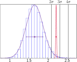
In Table 7, we present results for $\varepsilon_{K}^{\text{SM}}$ obtained using the FLAG average for $\hat{B}_{K}$ Aoki et al. (2013) and $V_{cb}$ from both inclusive Alberti et al. (2015) and exclusive channels Bailey et al. (2014a). The corresponding probability distributions for $\varepsilon_{K}^{\text{SM}}$ and $\varepsilon_{K}^{\text{Exp}}$ are presented in Fig. 2. The corresponding results for $\Delta\varepsilon_{K}$ are presented in Table 8.

Table 7: $\varepsilon_{K}^{\text{SM}}$ in units of $10^{-3}$. Here, we use the FLAG average for $\hat{B}_{K}$ in Table 3. The input methods of CKMfitter, UTfit, and AOF represent different inputs for the Wolfenstein parameters, which are explained in detail in Section III.1.

Input Method	Inclusive $V_{cb}$	Exclusive $V_{cb}$
CKMfitter	$2.31(23)$	$1.73(18)$
UTfit	$2.30(24)$	$1.73(19)$
AOF	$2.15(23)$	$1.61(18)$

Table 8: $\Delta\varepsilon_{K}$. Here, we use $\varepsilon_{K}^{\text{SM}}$ from Table 7. We obtain $\sigma$ by combining the errors of $\varepsilon_{K}^{\text{SM}}$ and $\varepsilon_{K}^{\text{Exp}}$ in quadrature.

Input Method	Inclusive $V_{cb}$	Exclusive $V_{cb}$
CKMfitter	$-0.34\sigma$	$2.7\sigma$
UTfit	$-0.31\sigma$	$2.7\sigma$
AOF	$0.33\sigma$	$3.4\sigma$

(a) CKMfitter

(b) UTfit

(c) AOF

(d) CKMfitter

(e) UTfit

(f) AOF

Figure 2: Gaussian probability distributions for $\varepsilon_{K}^{\text{SM}}$ (blue dotted line) and $\varepsilon_{K}^{\text{Exp}}$ (red solid line). Here, the results are obtained using the FLAG $\hat{B}_{K}$. The results of 2(a), 2(b), and 2(c) are obtained using the inclusive $V_{cb}$. Those of 2(d), 2(e), and 2(f) are obtained using the exclusive $V_{cb}$.

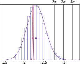
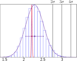
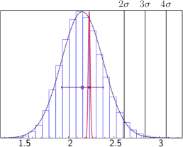
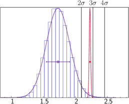
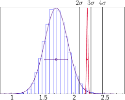
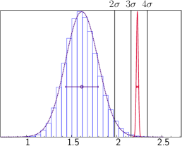
From Table 8, we find that $\varepsilon_{K}^{\text{SM}}$ with inclusive $V_{cb}$ is consistent with $\varepsilon_{K}^{\text{Exp}}$ within $1\sigma$. In other words, $\Delta\varepsilon_{K}$ is consistent with zero with inclusive $V_{cb}$ regardless of the input methods.

However, from Tables 7 and 8, $\varepsilon_{K}^{\text{SM}}$ with exclusive $V_{cb}$ is only 72% of $\varepsilon_{K}^{\text{Exp}}$. For this case, with the most reliable input method (AOF), $\Delta\varepsilon_{K}$ is $3.4\sigma$. Since the largest contribution in our estimate of $\varepsilon_{K}^{\text{SM}}$ that we neglect is much less than $2\%$, the neglected contributions cannot explain the gap $\Delta\varepsilon_{K}$ of 28% with exclusive $V_{cb}$. Hence, our final results for $\Delta\varepsilon_{K}$ are

$$\Delta\varepsilon_{K} =3.4\sigma \text{(exclusive $V_{cb}$)}\,,$$ (88)

$$\Delta\varepsilon_{K} =0.33\sigma \text{(inclusive $V_{cb}$)}\,,$$ (89)

where we take the AOF result as our quoted value.

In the case of the FLAG $\hat{B}_{K}$, the BMW result for $\hat{B}_{K}$ Durr et al. (2011) dominates the FLAG result, and the gauge ensembles used for the BMW calculation are independent of those used for the determination of exclusive $V_{cb}$ Bailey et al. (2014a) by the FNAL/MILC collaboration. Hence, we assume that we may neglect the correlation between the FLAG $\hat{B}_{K}$ and the exclusive $V_{cb}$. However, the SWME $\hat{B}_{K}$ calculation in Ref. Bae et al. (2014b) shares the same MILC gauge ensembles with the exclusive $V_{cb}$ determination in Ref. Bailey et al. (2014a). Hence, in this case, we cannot neglect the correlation between the SWME $\hat{B}_{K}$ and the exclusive $V_{cb}$. We introduce $+50\%$ correlation and $-50\%$ anti-correlation between the SWME $\hat{B}_{K}$ and the exclusive $V_{cb}$, and take the maximum deviation from the uncorrelated case as the systematic error due to the unknown correlation between them. The details of this analysis are explained in Appendix B. However, this analysis shows that the size of the ambiguity due to the correlation between the SWME $\hat{B}_{K}$ and the exclusive $V_{cb}$ is so large that we can use the results of the SWME $\hat{B}_{K}$ only to cross-check those with the FLAG $\hat{B}_{K}$. This analysis of the correlation is another update from the previous paper Bailey et al. (2014b).

Figure 3: Recent history of $\Delta\varepsilon_{K}$ along with the theoretical progress.

It is interesting to understand the historical evolution of $\Delta\varepsilon_{K}/\sigma$ along with the theoretical progress in lattice QCD and perturbative QCD. In Fig. 3, we present $\Delta\varepsilon_{K}/\sigma$ as a function of time. In 2012, the RBC/UKQCD collaboration reported $\xi_{0}$ in Ref. Blum et al. (2012). In addition to this, using the LLV average for $\hat{B}_{K}$ Laiho et al. (2010), the SWME collaboration reported $\Delta\varepsilon_{K}=2.5\sigma$ in Ref. Jang and Lee (2012) in 2012. In 2014, FNAL/MILC reported an updated $V_{cb}$ in the exclusive channel. Using the FLAG average for $\hat{B}_{K}$ Aoki et al. (2013) and the NNLO value of $\eta_{ct}$ Brod and Gorbahn (2010), the SWME collaboration reported the updated $\Delta\varepsilon_{K}=3.0\sigma$ in Ref. Bailey et al. (2014b) in 2014. In this paper, we investigate issues in the NNLO calculation of $\eta_{cc}$ Brod and Gorbahn (2012); Buras and Girrbach (2013) and use the SWME result in Table 5 to report the updated $\Delta\varepsilon_{K}=3.4\sigma$ in Eq. (88).

V Conclusion

In this paper, we observe that there is a substantial $3.4\sigma$ tension in $\varepsilon_{K}$ between experiment and the SM theory with lattice QCD inputs. For this claim, we choose the angle-only fit (AOF), the exclusive $V_{cb}$ (lattice QCD results), and the FLAG $\hat{B}_{K}$ (lattice QCD results) to determine the final value. We choose the AOF method to determine the final result because the AOF Wolfenstein parameters do not have unwanted correlation with $\varepsilon_{K}$ and $\hat{B}_{K}$. However, the tension disappears in the case of inclusive $V_{cb}$ (results of the heavy quark expansion based on the OPE) regardless of the choices for the Wolfenstein parameters.

In Table 9, we present the error budget of $\varepsilon_{K}^{\text{SM}}$ for the central value. This is obtained using the error propagation method explained in Section III.2. From this error budget, we find out that $V_{cb}$ dominates the error in $\varepsilon_{K}^{\text{SM}}$. Hence, it is essential to reduce the error of $V_{cb}$ as much as possible. (See also Refs. Buras et al. (2014); Buras and Girrbach (2014).) In order to achieve this goal, we plan to extract $V_{cb}$ from the exclusive channel using the Oktay-Kronfeld (OK) action Oktay and Kronfeld (2008) for heavy quarks to calculate the form factors for $\bar{B}\to D^{(*)}\ell\bar{\nu}$ decays. Preliminary results in the early stage of the $V_{cb}$ project are reported in Refs. Jang et al. (2014); Bailey et al. (2014c, d).

Table 9: Error budget for $\varepsilon_{K}^{\text{SM}}$ obtained using the AOF method, the exclusive $V_{cb}$, and the FLAG $\hat{B}_{K}$. Here, the values are fractional contributions to the total error obtained using the formula in Eq. (86).

source	error (%)	memo
$V_{cb}$	39.3	FNAL/MILC
$\bar{\eta}$	20.4	AOF
$\eta_{ct}$	16.9	$c-t$ Box
$\eta_{cc}$	7.1	$c-c$ Box
$\bar{\rho}$	5.4	AOF
$m_{t}$	2.4
$\xi_{0}$	2.2	RBC/UKQCD
$\xi_{\text{LD}}$	2.0	RBC/UKQCD
$\hat{B}_{K}$	1.5	FLAG
$m_{c}$	1.0
$\vdots$	$\vdots$

Our results for $\eta_{cc}$ are consistent with the conclusion of Ref. Brod and Gorbahn (2012) regarding the convergence of perturbation theory. Uncertainty due to truncated higher order terms requires further investigation in the future. Lattice QCD calculations with dynamical charm quarks, such as that envisioned by the RBC/UKQCD collaboration, could shed light on this issue.

We expect that our results for $\varepsilon_{K}$ would be consistent with those from a global UT analysis, such as that in Ref. Laiho et al. (2010). The authors of Ref. Laiho et al. (2010) performed one analysis with inclusive $V_{cb}$ and another analysis with exclusive $V_{cb}$ instead of inflating their errors and taking the average. In this respect, the analysis of Ref. Laiho et al. (2010) is different from those of UTfit and CKMfitter. Such a global analysis with up-to-date inputs from lattice QCD has not been performed yet. It would be interesting to see the results of such an analysis.

Appendix A Next-to-next-to leading order $\eta_{cc}$

We will begin from the master formula for $\eta_{cc}$ Brod and Gorbahn (2012) and give an explicit expression for each component which is necessary for a numerical evaluation. For $\mu\leq\mu_{c}$,

$$\eta_{cc}=\frac{1}{m_{c}^{2}\left(m_{c}\right)}\tilde{C}_{S2}^{cc}\left(\mu_{c}\right)\left[\alpha_{s}\left(\mu_{c},3\right)\right]^{a_{+}(3)}K_{+}^{-1}(\mu_{c},3)\,.$$ (90)

The magic number $a_{+}(3)=2/9$ can be obtained from Eq. (121). $\alpha_{s}(\mu,f)$ is the running strong coupling constant with $f$ active flavors at scale $\mu$. We will use the four-loop $\alpha_{s}$ running formula Chetyrkin et al. (2000, 1997). The Wilson coefficient $\tilde{C}_{S2}^{cc}(\mu_{c})$ of the $\Delta S=2$ four-fermion operator is defined by Eq. (91). The running matrix $K_{+}^{-1}(\mu_{c},3)$ is given by Eq. (A).

At the charm scale $\mu_{c}$, the effective four flavor theory is matched to the effective three flavor theory by requiring the following condition Brod and Gorbahn (2012),

$$\sum_{i,j=+,-}C_{i}C_{j}\langle Q_{i}Q_{j}\rangle=\frac{1}{8\pi^{2}}{\tilde{C}}_{S2}^{cc}\langle{\tilde{Q}}_{S2}\rangle\,.$$ (91)

The matrix elements and the Wilson coefficients are expanded in the three flavor strong coupling $\alpha_{s}(\mu_{c},3)$,

$$\langle{\tilde{Q}}_{S2}\rangle= \tilde{r}_{S2}\langle{\tilde{Q}}_{S2}\rangle^{(0)}\,,$$ (92)

$$\tilde{r}_{S2}= 1+\frac{\alpha_{s}(\mu_{c},3)}{4\pi}\tilde{r}_{S2}^{(1)}+\left(\frac{\alpha_{s}(\mu_{c},3)}{4\pi}\right)^{2}\tilde{r}_{S2}^{(2)}\,,$$ (93)

$$\langle Q_{i}Q_{j}\rangle= \frac{m_{c}^{2}(\mu_{c})}{8\pi^{2}}d_{ij}\langle{\tilde{Q}}_{S2}\rangle^{(0)}\,,$$ (94)

$$d_{ij}= d_{ij}^{(0)}+\frac{\alpha_{s}(\mu_{c},3)}{4\pi}d_{ij}^{(1)}+\left(\frac{\alpha_{s}(\mu_{c},3)}{4\pi}\right)^{2}d_{ij}^{(2)}\,,$$ (95)

$$C_{i}(\mu_{c})= C_{i}^{(0)}(\mu_{c})+\frac{\alpha_{s}(\mu_{c},3)}{4\pi}C_{i}^{(1)}(\mu_{c})$$

$$+\left(\frac{\alpha_{s}(\mu_{c},3)}{4\pi}\right)^{2}C_{i}^{(2)}(\mu_{c})\,,$$ (96)

$$\tilde{C}_{S2}^{cc}(\mu_{c})= \tilde{C}_{S2}^{cc(0)}(\mu_{c})+\frac{\alpha_{s}(\mu_{c},3)}{4\pi}\tilde{C}_{S2}^{cc(1)}(\mu_{c})$$

$$+\left(\frac{\alpha_{s}(\mu_{c},3)}{4\pi}\right)^{2}\tilde{C}_{S2}^{cc(2)}(\mu_{c})\,.$$ (97)

Then, the matching results are

$$\tilde{C}_{S2}^{cc(0)}(\mu_{c})= m_{c}^{2}(\mu_{c})C_{i}^{(0)}C_{j}^{(0)}d_{ij}^{(0)}\,,$$ (98)

$$\tilde{C}_{S2}^{cc(1)}(\mu_{c})= m_{c}^{2}(\mu_{c})\bigg{[}C_{i}^{(0)}C_{j}^{(0)}\hat{d}_{ij}^{(1)}$$

$$+\big{(}C_{i}^{(1)}C_{j}^{(0)}+C_{i}^{(0)}C_{j}^{(1)}\big{)}d_{ij}^{(0)}\bigg{]}\,,$$ (99)

$$\tilde{C}_{S2}^{cc(2)}(\mu_{c})= m_{c}^{2}(\mu_{c})\bigg{[}C_{i}^{(0)}C_{j}^{(0)}\left(\hat{d}_{ij}^{(2)}+\frac{2}{3}\log\frac{\mu_{c}^{2}}{m_{c}^{2}}d_{ij}^{(1)}\right)$$

$$+\big{(}C_{i}^{(1)}C_{j}^{(0)}+C_{i}^{(0)}C_{j}^{(1)}\big{)}\left(\hat{d}_{ij}^{(1)}+\frac{2}{3}\log\frac{\mu_{c}^{2}}{m_{c}^{2}}d_{ij}^{(0)}\right)$$

$$+\big{(}C_{i}^{(2)}C_{j}^{(0)}+C_{i}^{(1)}C_{j}^{(1)}+C_{i}^{(0)}C_{j}^{(2)}\big{)}d_{ij}^{(0)}\bigg{]}\,,$$ (100)

where $m_{c}=m_{c}(m_{c})$ in the logarithms multiplied by $d_{ij}^{(0,1)}$, and

$$\hat{d}_{ij}^{(1)}\equiv d_{ij}^{(1)}-d_{ij}^{(0)}\tilde{r}_{S2}^{(1)}\,,$$ (101)

$$\hat{d}_{ij}^{(2)}\equiv d_{ij}^{(2)}-\hat{d}_{ij}^{(1)}\tilde{r}_{S2}^{(1)}-d_{ij}^{(0)}\tilde{r}_{S2}^{(2)}\,.$$ (102)

Note that the matching scale is the charm quark mass $\mu_{c}=m_{c}(m_{c})$; in Eqs. (98), (99), and (100), the Wilson coefficients $C_{i}^{(l)}(\mu_{c})\ (l=0,1,2\,;i=\pm)$ are evaluated at $\mu_{c}=m_{c}$,

$$C_{i}^{(l)}=C_{i}^{(l)}(m_{c})\,.$$ (103)

These are obtained by renormalization group evolution from the scale $\mu_{W}$ down to the scale $\mu_{c}=m_{c}$. (See Eq. (134).) To examine the size of residual scale dependence, we vary $\mu_{c}$, keeping the condition Eq. (103).

Then the residual scale $\mu_{c}$ dependence in $\tilde{C}_{S2}^{(l)}(\mu_{c})$ enters from logarithms which are shown explicitly in Eq. (100) and through $d_{ij}^{(l)}$ and $\tilde{r}_{S2}^{(l)}$; it also comes from the expansion $m_{c}(\mu_{c})$. The expansion of the charm quark mass $m_{c}(\mu_{c})$ near $\mu_{c}=m_{c}$ is given by Eq. (137) with $f=4$. The resulting residual scale dependence in $\eta_{cc}$ can be seen from Fig. 4.

The leading and next-to-leading order (NLO) calculations can be found from Ref. Herrlich and Nierste (1994), with the number of colors $N_{c}=3$, $l_{c}=\log\left(\mu_{c}^{2}/m_{c}^{2}\left(\mu_{c}\right)\right)$,

$$d_{++}^{(0)}=\frac{3}{2}\,,$$

$$d_{+-}^{(0)}=d_{-+}^{(0)}=-\frac{1}{2}\,,$$

$$d_{--}^{(0)}=\frac{1}{2}\,,$$ (104)

$$d_{++}^{(1)}=9l_{c}-\frac{27}{2}-\frac{\pi^{2}}{6}\,,$$

$$d_{+-}^{(1)}=d_{-+}^{(1)}=-6l_{c}-\frac{23}{6}+\frac{5\pi^{2}}{18}\,,$$

$$d_{--}^{(1)}=6l_{c}+\frac{53}{6}+\frac{\pi^{2}}{18}\,,$$ (105)

$$\tilde{r}_{S2}^{(1)}=-\frac{17}{3}\,.$$ (106)

The next-to-next-to-leading order (NNLO) calculation results are presented in Ref. Brod and Gorbahn (2012),

$$\hat{d}_{++}^{(2)}= \frac{1665873233}{8164800}-\frac{1573}{162}B_{4}-\frac{133}{72}D_{3}$$

$$+\frac{49}{36}\zeta_{2}l_{c}+\frac{4313}{216}l_{c}^{2}-\frac{15059}{1296}l_{c}$$

$$+\frac{210213}{560}S_{2}-\frac{1501}{54}\zeta_{2}^{2}-\frac{7567241}{204120}\zeta_{2}$$

$$-\frac{1697893}{7776}\zeta_{3}+\frac{11575}{216}\zeta_{4}\,,$$ (107)

$$\hat{d}_{+-}^{(2)}=\hat{d}_{-+}^{(2)}= \frac{87537463}{1166400}+\frac{685}{162}B_{4}-\frac{83}{72}D_{3}$$

$$+\frac{695}{36}\zeta_{2}l_{c}-\frac{1475}{216}l_{c}^{2}-\frac{57763}{1296}l_{c}$$

$$-\frac{4797}{80}S_{2}-\frac{791}{54}\zeta_{2}^{2}+\frac{366569}{29160}\zeta_{2}$$

$$+\frac{57673}{7776}\zeta_{3}-\frac{4999}{216}\zeta_{4}\,,$$ (108)

$$\hat{d}_{--}^{(2)}= \frac{2129775941}{8164800}+\frac{491}{162}B_{4}+\frac{11}{72}D_{3}$$

$$+\frac{865}{36}\zeta_{2}l_{c}+\frac{12533}{216}l_{c}^{2}+\frac{171121}{1296}l_{c}$$

$$+\frac{59121}{560}S_{2}-\frac{517}{54}\zeta_{2}^{2}+\frac{9261883}{204120}\zeta_{2}$$

$$-\frac{411709}{7776}\zeta_{3}-\frac{7913}{216}\zeta_{4}\,.$$ (109)

Some constants for the master integrals are Steinhauser (2001)

$$D_{3}= 6\zeta_{3}-\frac{15}{4}\zeta_{4}-6\left[\mathrm{Cl}_{2}\left(\frac{\pi}{3}\right)\right]^{2}\,,$$

$$B_{4}= -4\zeta_{2}\ln^{2}{2}+\frac{2}{3}\ln^{4}{2}-\frac{13}{2}\zeta_{4}+16\mathrm{Li}_{4}\left(\frac{1}{2}\right)\,,$$

$$S_{2}= \frac{4}{9\sqrt{3}}\mathrm{Cl}_{2}\left(\frac{\pi}{3}\right)\,,$$ (110)

with

$$\mathrm{Cl}_{2}(x)= \mathrm{Im}\left(\mathrm{Li}_{2}(e^{ix})\right)\,,$$ (111)

$$\mathrm{Li}_{n}(z)= \sum_{k=1}^{\infty}\frac{z^{k}}{k^{n}}\,,$$ (112)

and the Riemann zeta function is

$$\zeta_{n}=\sum_{k=1}^{\infty}\frac{1}{k^{n}}\,.$$ (113)

In numerical evaluation, we use approximated numbers which are obtained using Mathematica.

$$\zeta_{2}= 1.644934\ldots=\frac{\pi^{2}}{6}\,,$$

$$\zeta_{3}= 1.202056\ldots\,,$$

$$\zeta_{4}= 1.082323\ldots=\frac{\pi^{4}}{90}\,,$$

$$\mathrm{Li}_{4}\left(\frac{1}{2}\right)= 0.5174790\ldots\,,$$

$$\mathrm{Cl}_{2}\left(\frac{\pi}{3}\right)= 1.014941\ldots\,.$$ (114)

For $\zeta_{2}$ and $\zeta_{4}$, we also give the exact expression.

The renormalization group evolution of the Wilson coefficients $C_{\pm}$ is described by the evolution matrix $U_{ij}$ Gorbahn and Haisch (2005),

$$C_{i}(\mu)=U_{ij}(\mu,\mu_{0})C_{j}(\mu_{0})\,,$$ (115)

which is diagonalized by the specific choice of evanescent operators,

$$U_{ij}(\mu,\mu_{0})=K_{i}(\mu)\left(\frac{\alpha_{s}(\mu_{0},f)}{\alpha_{s}(\mu,f)}\right)^{a_{i}}K_{i}^{-1}(\mu_{0})\delta_{ij}\,,$$ (116)

where

$$K_{\pm}(\mu)= 1+\frac{\alpha_{s}(\mu,f)}{4\pi}J_{\pm}^{(1)}+\Big{(}\frac{\alpha_{s}(\mu,f)}{4\pi}\Big{)}^{2}J_{\pm}^{(2)}\,,$$ (117)

$$K_{\pm}^{-1}(\mu_{0})= 1-\frac{\alpha_{s}(\mu_{0},f)}{4\pi}J_{\pm}^{(1)}$$

$$-\Big{(}\frac{\alpha_{s}(\mu_{0},f)}{4\pi}\Big{)}^{2}\big{(}J_{\pm}^{(2)}-(J_{\pm}^{(1)})^{2}\big{)}\,,$$ (118)

and

$$J_{\pm}^{(1)}= \frac{\beta_{1}}{\beta_{0}}a_{\pm}-\frac{\gamma_{\pm}^{(1)}}{2\beta_{0}}\,,$$ (119)

$$J_{\pm}^{(2)}= \frac{\beta_{2}}{2\beta_{0}}a_{\pm}+\frac{1}{2}\left((J_{\pm}^{(1)})^{2}-\frac{\beta_{1}}{\beta_{0}}J_{\pm}^{(1)}\right)-\frac{\gamma_{\pm}^{(2)}}{4\beta_{0}}\,.$$ (120)

The expansion coefficients of the QCD beta function $\beta_{i}$ are given in Eq. (A). The anomalous dimensions $\gamma_{\pm}^{(i)}$ for the operators $Q_{\pm}$ are taken from Ref. Buras et al. (2006),

$$\gamma_{\pm}^{(0)} =\pm 6\left(1\mp\frac{1}{3}\right)=2\beta_{0}a_{\pm}\,,$$ (121)

$$\gamma_{\pm}^{(1)} =\left(-\frac{21}{2}\pm\frac{2}{3}f\right)\left(1\mp\frac{1}{3}\right)\,,$$ (122)

$$\gamma_{\pm}^{(2)} =\frac{1}{300}\left(349049\pm 201485\right)-\frac{1}{1350}\left(115577\mp 9795\right)f$$

$$\mp\frac{130}{27}\left(1\mp\frac{1}{3}\right)f^{2}\mp\left(672+80\left(1\mp\frac{1}{3}\right)f\right)\zeta_{3}\,.$$ (123)

The number of active flavors is fixed while applying Eq. (115). The number of flavors is implied by the strong coupling constant in Eq. (116).

The initial conditions for the Wilson coefficients $C_{\pm}$ are chosen at the scale $\mu_{W}$,

$$C_{\pm}(\mu_{W})= C_{\pm}^{(0)}(\mu_{W})+\frac{\alpha_{s}(\mu_{W},5)}{4\pi}C_{\pm}^{(1)}(\mu_{W})$$

$$+\left(\frac{\alpha_{s}(\mu_{W},5)}{4\pi}\right)^{2}C_{\pm}^{(2)}(\mu_{W})\,.$$ (124)

The expansion coefficients are given in Ref. Buras et al. (2006),

$$C_{\pm}^{(0)}(\mu_{W})= 1\,,$$

$$C_{\pm}^{(1)}(\mu_{W})= \pm\frac{1}{2}\left(1\mp\frac{1}{3}\right)\left(11+6\ln\frac{\mu_{W}^{2}}{M_{W}^{2}}\right)\,,$$

$$C_{\pm}^{(2)}(\mu_{W})= -\frac{1}{3600}(135677\mp 124095)$$

$$+\frac{1}{18}(7\pm 51)\pi^{2}\mp\frac{1}{2}\left(1\mp\frac{1}{3}\right)T(x_{t})$$

$$-\frac{5}{36}(11\mp 249)\ln\frac{\mu_{W}^{2}}{M_{W}^{2}}+\frac{1}{6}(7\pm 51)\ln^{2}\frac{\mu_{W}^{2}}{M_{W}^{2}}\,,$$ (125)

where

$$T(x_{t})= \frac{112}{9}+32x_{t}+\left(\frac{20}{3}+16x_{t}\right)\ln x_{t}$$

$$-(8+16x_{t})\sqrt{4x_{t}-1}\mathrm{Cl}_{2}\left(2\arcsin\left(\frac{1}{2\sqrt{x_{t}}}\right)\right)\,,$$ (126)

$x_{t}=m_{t}^{2}(\mu_{W})/M_{W}^{2}$, and $\mathrm{Cl}_{2}(x)$ is given in Eq. (111).

In numerical evaluation, we use an approximated number which is obtained using Mathematica,

$$\mathrm{Cl}_{2}\left(2\arcsin\left(\frac{1}{2\sqrt{x_{t}}}\right)\right)=0.8464504\ldots$$ (127)

The value $x_{t}$ is evaluated with the top quark mass $m_{t}(m_{t})=163.3\;\mathrm{GeV}$ and $M_{W}=80.385\;\mathrm{GeV}$, approximating $m_{t}(\mu_{W})=m_{t}(m_{t})$.

Running from $\mu_{W}$ to the bottom quark threshold $\mu_{b}$ is achieved by

$$C_{i}(\mu_{b},5)= K_{i}(\mu_{b},5)\left(\frac{\alpha_{s}(\mu_{W},5)}{\alpha_{s}(\mu_{b},5)}\right)^{a_{i}(5)}K_{i}^{-1}(\mu_{W},5)C_{i}(\mu_{W})$$

$$= C_{i}^{(0)}(\mu_{b},5)+\frac{\alpha_{s}(\mu_{b},5)}{4\pi}C_{i}^{(1)}(\mu_{b},5)$$

$$+\left(\frac{\alpha_{s}(\mu_{b},5)}{4\pi}\right)^{2}C_{i}^{(2)}(\mu_{b},5)\,.$$ (128)

The threshold correction at $\mu_{b}$ is given by the following. Writing

$$C_{i}(\mu_{b},4)= C_{i}^{(0)}(\mu_{b},4)+\frac{\alpha_{s}(\mu_{b},4)}{4\pi}C_{i}^{(1)}(\mu_{b},4)$$

$$+\left(\frac{\alpha_{s}(\mu_{b},4)}{4\pi}\right)^{2}C_{i}^{(2)}(\mu_{b},4)\,,$$ (129)

then

$$C_{i}^{(0)}(\mu_{b},4)= C_{i}^{(0)}(\mu_{b},5)\,,$$

$$C_{i}^{(1)}(\mu_{b},4)= C_{i}^{(1)}(\mu_{b},5)\,,$$

$$C_{i}^{(2)}(\mu_{b},4)= C_{i}^{(2)}(\mu_{b},5)-\delta C_{i}^{(2)}(\mu_{b})\,,$$ (130)

where

$$\delta C_{\pm}^{(2)}(\mu_{b})=-\frac{2}{3}\ln\frac{\mu_{b}^{2}}{m_{b}^{2}}C_{\pm}^{(1)}(\mu_{b},5)$$

$$-\left(\frac{2}{3}\ln\frac{\mu_{b}^{2}}{m_{b}^{2}}r_{\pm}^{(1)}(\mu_{b},5)+\delta r_{\pm}^{(2)}(\mu_{b})\right)C_{\pm}^{(0)}(\mu_{b},5)$$

$$=-\frac{2}{3}\ln\frac{\mu_{b}^{2}}{m_{b}^{2}}C_{\pm}^{(1)}(\mu_{b},5)$$

$$+\left(\pm\left(1\mp\frac{1}{3}\right)\left(\frac{59}{36}+\frac{1}{3}\ln\frac{\mu_{b}^{2}}{m_{b}^{2}}+\ln^{2}\frac{\mu_{b}^{2}}{m_{b}^{2}}\right)\right)C_{\pm}^{(0)}(\mu_{b},5)\,.$$ (131)

The definition of $r_{i}^{(1)}$ and $\delta r_{i}^{(2)}$, and their combination, the multiplicative factor of $C_{i}^{(0)}$, can be found in Ref. Buras et al. (2006).

Running from $\mu_{b}$ to the matching scale $\mu_{c}=m_{c}(m_{c})$ is achieved by

$$C_{i}(\mu_{c},4)= K_{i}(\mu_{c},4)\left(\frac{\alpha_{s}(\mu_{b},4)}{\alpha_{s}(\mu_{c},4)}\right)^{a_{i}(4)}K_{i}^{-1}(\mu_{b},4)C_{i}(\mu_{b},4)$$

$$= C_{i}^{(0)}(\mu_{c},4)+\frac{\alpha_{s}(\mu_{c},4)}{4\pi}C_{i}^{(1)}(\mu_{c},4)$$

$$+\left(\frac{\alpha_{s}(\mu_{c},4)}{4\pi}\right)^{2}C_{i}^{(2)}(\mu_{c},4)\,.$$ (132)

In the matching calculation, we need the expansion in the three flavor strong coupling, Eq. (A).

Equating $C_{i}(\mu_{c})$ in Eq. (A) to $C_{i}(\mu_{c},4)$ after applying Eq. (A) to the flavor threshold with $f=4$, then

$$C_{i}^{(0)}(\mu_{c})= C_{i}^{(0)}(\mu_{c},4)\,,$$

$$C_{i}^{(1)}(\mu_{c})= C_{i}^{(1)}(\mu_{c},4)\,,$$

$$C_{i}^{(2)}(\mu_{c})= C_{i}^{(2)}(\mu_{c},4)+\frac{2}{3}\ln\frac{\mu_{c}^{2}}{m_{c}^{2}}C_{i}^{(1)}(\mu_{c},4)\,.$$ (133)

Hence, at the matching scale of the charm quark mass $\mu_{c}=m_{c}(m_{c})$, we obtain

$$C_{i}^{(l)}(m_{c})=C_{i}^{(l)}(m_{c},4)\,,\quad(l=0,1,2)\,.$$ (134)

The QCD beta function expansion coefficients $\beta_{i}$ to four-loop order are Buras et al. (2006); Chetyrkin et al. (2000):

$$\beta_{0}= 11-\frac{2}{3}f\,,$$

$$\beta_{1}= 102-\frac{38}{3}f\,,$$

$$\beta_{2}= \frac{2857}{2}-\frac{5033}{18}f+\frac{325}{54}f^{2}\,,$$

$$\beta_{3}= \frac{149753}{6}+3564\zeta_{3}-\left(\frac{1078361}{162}+\frac{6508}{27}\zeta_{3}\right)f$$

$$+\left(\frac{50065}{162}+\frac{6472}{81}\zeta_{3}\right)f^{2}+\frac{1093}{729}f^{3}\,.$$ (135)

The NNNLO decoupling relation of the strong coupling constant at a flavor threshold $\mu$ is Chetyrkin et al. (2000)

$$\frac{\alpha_{s}(\mu,f-1)}{4\pi}$$

$$= \frac{\alpha_{s}(\mu,f)}{4\pi}-\left(\frac{\alpha_{s}(\mu,f)}{4\pi}\right)^{2}\frac{2}{3}\ln\frac{\mu^{2}}{m_{h}^{2}}$$

$$+\left(\frac{\alpha_{s}(\mu,f)}{4\pi}\right)^{3}\left(\frac{22}{9}-\frac{38}{3}\ln\frac{\mu^{2}}{m_{h}^{2}}+\frac{4}{9}\ln^{2}\frac{\mu^{2}}{m_{h}^{2}}\right)$$

$$+\left(\frac{\alpha_{s}(\mu,f)}{4\pi}\right)^{4}\bigg{(}\frac{564731}{1944}-\frac{2633}{486}(f-1)-\frac{82043}{432}\zeta_{3}$$

$$\quad+\frac{1}{27}\ln\frac{\mu^{2}}{m_{h}^{2}}(-6793+281(f-1))$$

$$\quad-\frac{131}{9}\ln^{2}\frac{\mu^{2}}{m_{h}^{2}}-\frac{8}{27}\ln^{3}\frac{\mu^{2}}{m_{h}^{2}}\bigg{)}\,,$$ (136)

where $m_{h}=m_{h}(m_{h})$ is the scale invariant $\overline{\text{MS}}$ mass of the heavy flavor which is removed from an effective theory below the threshold $\mu$, and $\zeta_{3}$ is a Riemann zeta function, Eq. (113).

The running quark mass $m_{q}(\mu)$, an $\overline{\text{MS}}$ mass at scale $\mu$, for a fixed number of active flavors $f$ is Chetyrkin et al. (2000)

$$\frac{m_{q}(\mu)}{m_{q}(\mu_{0})}=\frac{R(\alpha_{s}(\mu)/4\pi)}{R(\alpha_{s}(\mu_{0})/4\pi)}\,,$$ (137)

with

$$R(x)= x^{c_{0}}\Bigg{\{}1+(c_{1}-b_{1}c_{0})x$$

$$+\frac{1}{2}\left[(c_{1}-b_{1}c_{0})^{2}+c_{2}-b_{1}c_{1}+b_{1}^{2}c_{0}-b_{2}c_{0}\right]x^{2}$$

$$+\bigg{[}\frac{1}{6}(c_{1}-b_{1}c_{0})^{3}$$

$$\quad+\frac{1}{2}(c_{1}-b_{1}c_{0})(c_{2}-b_{1}c_{1}+b_{1}^{2}c_{0}-b_{2}c_{0})$$

$$\quad+\frac{1}{3}(c_{3}-b_{1}c_{2}+b_{1}^{2}c_{1}-b_{2}c_{1}-b_{1}^{3}c_{0}$$

$$\quad+2b_{1}b_{2}c_{0}-b_{3}c_{0})\bigg{]}x^{3}\Bigg{\}}\,,$$ (138)

where $m_{q}(\mu_{0})$ is the scale invariant mass $m_{q}=m_{q}(m_{q})$, $b_{i}=\beta_{i}/\beta_{0}$, and $c_{i}=\gamma_{m}^{(i)}/\beta_{0}$. The QCD beta function coefficients $\beta_{i}$ are given in Eq. (A). The mass anomalous dimensions $\gamma_{m}^{(i)}$ are known up to four-loop order,

$$\gamma_{m}^{(0)}= 4\,,$$

$$\gamma_{m}^{(1)}= \frac{202}{3}-\frac{20}{9}f\,,$$

$$\gamma_{m}^{(2)}= 1249-\left(\frac{2216}{27}+\frac{160}{3}\zeta_{3}\right)f-\frac{140}{81}f^{2}\,,$$

$$\gamma_{m}^{(3)}= \frac{4603055}{162}+\frac{135680}{27}\zeta_{3}-8800\zeta_{5}$$

$$+\left(-\frac{91723}{27}-\frac{34192}{9}\zeta_{3}+880\zeta_{4}+\frac{18400}{9}\zeta_{5}\right)f$$

$$+\left(\frac{5242}{243}+\frac{800}{9}\zeta_{3}-\frac{160}{3}\zeta_{4}\right)f^{2}+\left(-\frac{332}{243}+\frac{64}{27}\zeta_{3}\right)f^{3}\,.$$ (139)

In numerical evaluation, we use approximated numbers for the Riemann zeta functions $\zeta_{n}$ which are obtained using Mathematica,

$$\zeta_{5}= 1.036927\ldots\,,$$ (140)

and $\zeta_{3}$ and $\zeta_{4}$ are given in Eq. (A).

We used Eq. (137) to expand the charm quark mass about $m_{c}=m_{c}(m_{c})$ with $f=4$.

Here, we will give numerical results for an initial scale $\mu_{W}=80\;\mathrm{GeV}$ and a varying charm scale $\mu_{c}$, $1.0\leq\mu_{c}\leq 2.0\;\mathrm{GeV}$. To examine the dependence on the scale $\mu_{W}$, we repeat the same analysis with $\mu_{W}=40,160\;\mathrm{GeV}$. The dependence on $\mu_{b}$ and $m_{t}(m_{t})$ is ignored Brod and Gorbahn (2012). Fig. 4 summarizes these results. The following are kept fixed for all analyses: the gauge boson masses $M_{Z}=91.1876\;\mathrm{GeV}\,,M_{W}=80.385\;\mathrm{GeV}$; quark masses $m_{t}(m_{t})=163.3\;\mathrm{GeV}\,,m_{b}(m_{b})=4.163\;\mathrm{GeV}\,,m_{c}(m_{c})=1.279\;\mathrm{GeV}$; bottom quark threshold $\mu_{b}=5.0\;\mathrm{GeV}$; and the strong coupling constant that provides an initial value for the running formula, $\alpha_{s}(M_{Z},5)=0.1184\;\mathrm{GeV}$.

Figure 4: Scale $\mu_{c}$ dependence of $\eta_{cc}$. Dotted, solid, and dashed lines represent results for $\mu_{W}=40,\ 80$, and $160\;\mathrm{GeV}$, respectively. The upper three (red) lines are the NNLO results, and the lower three (purple) lines are the NLO results.

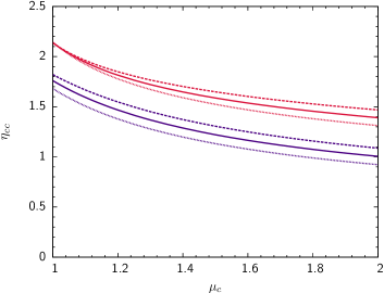
At the scales $\mu_{W}=80\;\mathrm{GeV}$ and $\mu_{c}=1.279\;\mathrm{GeV}$,

$$\eta_{cc}/[\alpha_{s}(\mu_{c},3)]^{a_{+}}= 1.129757+0.571608+0.430890\,,$$

$$\eta_{cc}^{\text{NNLO}}= 1.738396\,,$$

$$\eta_{cc}^{\text{NLO}}= 1.387098\,.$$ (141)

The value of $\eta_{cc}^{\text{NLO}}$ is obtained by summing the first two terms in the series, and the value of $\eta_{cc}^{\text{NNLO}}$ is obtained by summing all three terms in the series.

At the scales $\mu_{W}=80\;\mathrm{GeV}$ and $\mu_{c}=1.300\;\mathrm{GeV}$,

$$\eta_{cc}/[\alpha_{s}(\mu_{c},3)]^{a_{+}}= 1.113769+0.568911+0.433783\,,$$

$$\eta_{cc}^{\text{NNLO}}= 1.720690\,,$$

$$\eta_{cc}^{\text{NLO}}= 1.368023\,.$$ (142)

We claim the NNLO $\eta_{cc}$ is

$$\eta_{cc}^{\text{NNLO}}=1.72(27)\,.$$ (143)

The central value corresponds to the result with the scales $\mu_{c}=1.3\;\mathrm{GeV}$ and $\mu_{W}=80\;\mathrm{GeV}$. For the error, we add the $\mu_{c}$ and $\mu_{W}$ dependences in quadrature,

$$\delta_{\mu_{c}}= \eta_{cc}^{\text{NNLO}}(\mu_{c}=1.3\;\mathrm{GeV},\mu_{W}=80\;\mathrm{GeV})$$

$$\quad-\eta_{cc}^{\text{NNLO}}(\mu_{c}=1.8\;\mathrm{GeV},\mu_{W}=80\;\mathrm{GeV})$$

$$= 0.266\,,$$

$$\delta_{\mu_{W}}= (\eta_{cc}^{\text{NNLO}}(\mu_{c}=1.3\;\mathrm{GeV},\mu_{W}=160\;\mathrm{GeV})$$

$$\quad-\eta_{cc}^{\text{NNLO}}(\mu_{c}=1.3\;\mathrm{GeV},\mu_{W}=40\;\mathrm{GeV}))/2$$

$$= 0.047\,.$$ (144)

Though we include errors from the inputs $\alpha_{s}(M_{Z},5)$ and $m_{c}(m_{c})$, the final errors in Eq. (143) are not affected; we use the errors quoted in Ref. Brod and Gorbahn (2012):

$$\delta_{\alpha_{s}}=0.06\,,\quad\delta_{m_{c}}=0.01\,.$$ (145)

In Ref. Brod and Gorbahn (2012), the authors also added the absolute shift from the NLO value of $\eta_{cc}$. It is the main reason for their larger error,

$$\eta_{cc}^{\text{NNLO}}=1.87(76)\,.$$ (146)

The main concern for adding this shift is poor convergence of the $\alpha_{s}$ expansion for $\eta_{cc}$. We, however, take the view that the error from $\mu_{c}$ dependence suffices to estimate the size of higher order corrections.

Here, we would like to comment on our choice of $1.3\,\mathrm{GeV}\leq\mu_{c}\leq 1.8\,\mathrm{GeV}$. If we examine each order in the perturbative corrections of $\eta_{cc}$,

$$\eta_{cc} =1_{\text{(LO)}}+0.37_{\text{(NLO)}}+0.36_{\text{(NNLO)}}$$

$$=1.72\qquad\text{(SWME)}\,,$$ (147)

$$\eta_{cc} =1_{\text{(LO)}}+0.38_{\text{(NLO)}}+0.49_{\text{(NNLO)}}$$

$$=1.87\qquad\text{(Brod \& Gorbahn)}\,.$$ (148)

The error that we quote is 0.27, which is roughly equivalent to the size of the NNLO correction. If we take the interval $1\,\mathrm{GeV}\leq\mu_{c}\leq 2\,\mathrm{GeV}$ as suggested in Ref. Brod and Gorbahn (2012), the error becomes 0.42, which is larger than the NNLO correction. If we follow the procedure of Ref. Brod and Gorbahn (2012), we add the NNLO size of 0.36 to this in quadrature which leads to a total error of 0.55. This value is significantly larger than the size of the NNLO correction. This estimate becomes even larger than that of the NLO and NNLO corrections combined in quadrature. If we assume that perturbation theory is working, then it is already arguably conservative to choose the size of the NNLO correction as the systematic error due to truncated NNNLO terms. Hence, we believe that the error quoted in Ref. Brod and Gorbahn (2012) is somewhat overestimated.

In addition, in Ref. Buras and Girrbach (2013), Buras and Girrbach suggested that, if one chooses the interval $1.3\,\mathrm{GeV}\leq\mu_{c}\leq 1.8\,\mathrm{GeV}$, one can obtain their result for $\eta_{cc}$,

$$\eta_{cc}\approx 1.70(21)\,,$$ (149)

which is obtained indirectly through an estimate of the long distance contribution to $\Delta M_{K}$ based on a large $N$ QCD inspired model calculation. We have directly verified their claim.

Our result for $\eta_{cc}^{\text{NLO}}$ agrees with the value quoted in Ref. Brod and Gorbahn (2012)

$$\eta_{cc}^{\text{NLO}}=1.38(52)(07)(02)\,.$$ (150)

Appendix B $\varepsilon_{K}^{\text{SM}}$ with the SWME $\hat{B}_{K}$

Lattice results for the exclusive $V_{cb}$ Bailey et al. (2014a) and the SWME $\hat{B}_{K}$ Bae et al. (2014b) are obtained using overlapping subsets of the MILC asqtad gauge ensembles Bazavov et al. (2010). This implies that there exists a complicated, non-trivial correlation between them. It is possible to calculate, in principle, this correlation exactly from the data set. Unfortunately, this correlation is not available yet. Hence, the current situation is that we need to estimate the systematic error due to the unknown correlation between $\hat{B}_{K}$ and $V_{cb}$.

Here is our strategy. First, we take the uncorrelated case as the central value. Second, we introduce $+50\%$ correlation between $\hat{B}_{K}$ and $V_{cb}$ and obtain results for $\varepsilon_{K}^{\text{SM}}$. Third, we introduce $-50\%$ anti-correlation between $\hat{B}_{K}$ and $V_{cb}$ and repeat the analysis to obtain $\varepsilon_{K}^{\text{SM}}$. Fourth, we take the maximum deviation from the central value as the systematic error due to the unknown correlation between $\hat{B}_{K}$ and $V_{cb}$.

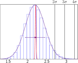
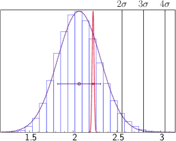
In Table 10, we present results for $\varepsilon_{K}^{\text{SM}}$ for the uncorrelated case. In Table 11, we present the corresponding results for $\Delta\varepsilon_{K}$. In Fig. 5, we show the corresponding probability distribution of $\varepsilon_{K}^{\text{SM}}$.

Table 10: $\varepsilon_{K}^{\text{SM}}$ in units of $10^{-3}$. We use the SWME $\hat{B}_{K}$ with no correlation between $\hat{B}_{K}$ and $V_{cb}$.

Input Method	Inclusive $V_{cb}$	Exclusive $V_{cb}$
CKMfitter	$2.22(25)$	$1.66(19)$
UTfit	$2.21(25)$	$1.66(20)$
AOF	$2.07(25)$	$1.55(19)$

Table 11: $\Delta\varepsilon_{K}$ with no correlation between $\hat{B}_{K}$ and $V_{cb}$. We take $\varepsilon_{K}^{\text{SM}}$ from Table 10. $\varepsilon_{K}^{\text{Exp}}$ is given in Eq. (I).

Input Method	Inclusive $V_{cb}$	Exclusive $V_{cb}$
CKMfitter	$0.04\sigma$	$2.9\sigma$
UTfit	$0.06\sigma$	$2.9\sigma$
AOF	$0.65\sigma$	$3.5\sigma$

(a) CKMfitter

(b) UTfit

(c) AOF

(d) CKMfitter

(e) UTfit

(f) AOF

Figure 5: Gaussian probability distributions for $\varepsilon_{K}^{\text{SM}}$ (blue dotted line) and $\varepsilon_{K}^{\text{Exp}}$ (red solid line) with the SWME $\hat{B}_{K}$. Here, we assume no correlation between $\hat{B}_{K}$ and $V_{cb}$. Results of 5(a), 5(b) and 5(c) are obtained using the inclusive $V_{cb}$. Results of 5(d), 5(e) and 5(f) are obtained using the exclusive $V_{cb}$.

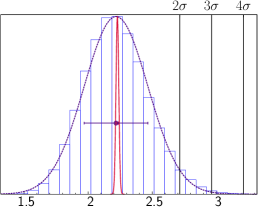
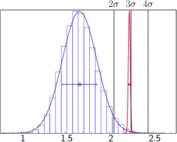
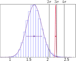
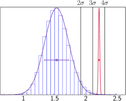
In Table 12, we present results for $\varepsilon_{K}^{\text{SM}}$ with $+50\%$ correlation and $-50\%$ anti-correlation between $\hat{B}_{K}$ and (exclusive) $V_{cb}$. In Table 13, we present the corresponding results for $\Delta\varepsilon_{K}$. In Fig. 6, we show the probability distribution for the corresponding $\varepsilon_{K}^{\text{SM}}$.

Table 12: $\varepsilon_{K}^{\text{SM}}$ in units of $10^{-3}$. We use the SWME $\hat{B}_{K}$ and the exclusive $V_{cb}$ with $+50\%$ correlation and $-50\%$ anti-correlation between them.

Input Method	$c=-50\%$	$c=+50\%$
CKMfitter	$1.66(17)$	$1.67(22)$
UTfit	$1.66(17)$	$1.66(22)$
AOF	$1.55(17)$	$1.55(21)$

Table 13: $\Delta\varepsilon_{K}$ with $+50\%$ correlation and $-50\%$ anti-correlation between $\hat{B}_{K}$ and exclusive $V_{cb}$. We take $\varepsilon_{K}^{\text{SM}}$ from Table 12. $\varepsilon_{K}^{\text{Exp}}$ is given in Eq. (I).

Input Method	$c=-50\%$	$c=+50\%$
CKMfitter	$3.4\sigma$	$2.6\sigma$
UTfit	$3.3\sigma$	$2.5\sigma$
AOF	$4.1\sigma$	$3.1\sigma$

(a) CKMfitter

(b) UTfit

(c) AOF

(d) CKMfitter

(e) UTfit

(f) AOF

Figure 6: Gaussian probability distributions for $\varepsilon_{K}^{\text{SM}}$ and $\varepsilon_{K}^{\text{Exp}}$ with the SWME $\hat{B}_{K}$ and exclusive $V_{cb}$. Results of 6(a), 6(b), and 6(c) are obtained with $-50\%$ anti-correlation between $\hat{B}_{K}$ and $V_{cb}$. Those of 6(d), 6(e), and 6(f) are obtained with $+50\%$ correlation between $\hat{B}_{K}$ and $V_{cb}$.

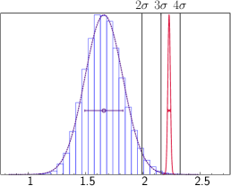
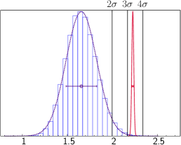
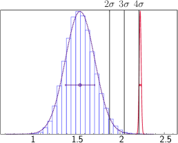
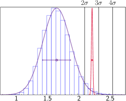
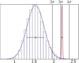
Hence, we obtain the final results for $\Delta\varepsilon_{K}$ for the SWME $\hat{B}_{K}$ and exclusive $V_{cb}$:

$$\Delta\varepsilon_{K} =(3.5\pm 0.6)\sigma\,,$$ (151)

where the error represents the uncertainty due to the correlation between $\hat{B}_{K}$ and exclusive $V_{cb}$.

First, the results in Eq. (151) are consistent with those in Eq. (88) within the systematic errors. Second, the correlation between $\hat{B}_{K}$ and exclusive $V_{cb}$ dominates the error in $\Delta\varepsilon_{K}$ with the SWME $\hat{B}_{K}$. In addition, this error is much larger than that in our final results in Eq. (88). Hence, we use the results with the SWME $\hat{B}_{K}$ only to cross-check those with the FLAG $\hat{B}_{K}$.

References

- Christenson et al. (1964) J. Christenson, J. Cronin, V. Fitch, and R. Turlay, Phys.Rev.Lett. 13, 138 (1964).
- Alavi-Harati et al. (1999) A. Alavi-Harati et al. (KTeV Collaboration), Phys.Rev.Lett. 83, 22 (1999), eprint hep-ex/9905060.
- Fanti et al. (1999) V. Fanti et al. (NA48 Collaboration), Phys.Lett. B465, 335 (1999), eprint hep-ex/9909022.
- Olive et al. (2014) K. Olive et al. (Particle Data Group), Chin.Phys. C38, 090001 (2014).
- Kobayashi and Maskawa (1973) M. Kobayashi and T. Maskawa, Prog.Theor.Phys. 49, 652 (1973).
- Cabibbo (1963) N. Cabibbo, Phys.Rev.Lett. 10, 531 (1963).
- Christ et al. (2013) N. Christ, T. Izubuchi, C. Sachrajda, A. Soni, and J. Yu (RBC and UKQCD Collaborations), Phys.Rev. D88, 014508 (2013), eprint 1212.5931.
- Christ et al. (2014) N. Christ, T. Izubuchi, C. T. Sachrajda, A. Soni, and J. Yu (RBC, UKQCD), PoS LATTICE2013, 397 (2014), eprint 1402.2577.
- Buras and Guadagnoli (2008) A. J. Buras and D. Guadagnoli, Phys.Rev. D78, 033005 (2008), eprint 0805.3887.
- Buras et al. (2010) A. J. Buras, D. Guadagnoli, and G. Isidori, Phys.Lett. B688, 309 (2010), eprint 1002.3612.
- Donoghue et al. (1992) J. Donoghue, E. Golowich, and B. R. Holstein, Dynamics of the standard model (Camb.Monogr.Part.Phys.Nucl.Phys.Cosmol., 1992).
- Aoki et al. (2013) S. Aoki, Y. Aoki, C. Bernard, T. Blum, G. Colangelo, et al. (2013), eprint 1310.8555.
- Bae et al. (2014a) T. Bae, Y.-C. Jang, H. Jeong, J. Kim, J. Kim, et al., PoS LATTICE2013, 476 (2014a), eprint 1310.7319.
- Arthur et al. (2013) R. Arthur et al. (RBC Collaboration, UKQCD Collaboration), Phys.Rev. D87, 094514 (2013), eprint 1208.4412.
- Laiho and Van de Water (2011) J. Laiho and R. S. Van de Water, PoS LATTICE2011, 293 (2011), eprint 1112.4861.
- Bae et al. (2012) T. Bae et al., Phys.Rev.Lett. 109, 041601 (2012), eprint 1111.5698.
- Durr et al. (2011) S. Durr, Z. Fodor, C. Hoelbling, et al., Phys.Lett. B705, 477 (2011), eprint 1106.3230.
- Bae et al. (2014b) T. Bae et al. (SWME Collaboration), Phys.Rev. D89, 074504 (2014b), eprint 1402.0048.
- Blum et al. (2012) T. Blum, P. Boyle, N. Christ, N. Garron, E. Goode, et al., Phys.Rev.Lett. 108, 141601 (2012), eprint 1111.1699.
- Bailey et al. (2014a) J. A. Bailey, A. Bazavov, C. Bernard, et al., Phys.Rev. D89, 114504 (2014a), eprint 1403.0635.
- Gambino and Schwanda (2014) P. Gambino and C. Schwanda, Phys.Rev. D89, 014022 (2014), eprint 1307.4551.
- Alberti et al. (2015) A. Alberti, P. Gambino, K. J. Healey, and S. Nandi, Phys.Rev.Lett. 114, 061802 (2015), eprint 1411.6560.
- Uraltsev (2000) N. Uraltsev (2000), eprint hep-ph/0010328.
- Buchalla et al. (1996) G. Buchalla, A. J. Buras, and M. E. Lautenbacher, Rev.Mod.Phys. 68, 1125 (1996), eprint hep-ph/9512380.
- Charles et al. (2005) J. Charles et al. (CKMfitter Group), Eur.Phys.J. C41, 1 (2005), eprint hep-ph/0406184.
- Hocker et al. (2001) A. Hocker, H. Lacker, S. Laplace, and F. Le Diberder, Eur.Phys.J. C21, 225 (2001), eprint hep-ph/0104062.
- Bona et al. (2005) M. Bona et al. (UTfit Collaboration), JHEP 0507, 028 (2005), eprint hep-ph/0501199.
- Bona et al. (2008) M. Bona et al. (UTfit Collaboration), JHEP 0803, 049 (2008), eprint 0707.0636.
- Bevan et al. (2013) A. Bevan, M. Bona, M. Ciuchini, D. Derkach, E. Franco, et al., Nucl.Phys.Proc.Suppl. 241-242, 89 (2013).
- Buras (1998) A. J. Buras, pp. 281–539 (1998), to appear in ’Probing the Standard Model of Particle Interactions’, F.David and R. Gupta, eds., 1998, Elsevier Science B.V., eprint hep-ph/9806471.
- Weisskopf and Wigner (1930a) V. Weisskopf and E. P. Wigner, Z.Phys. 63, 54 (1930a).
- Weisskopf and Wigner (1930b) V. Weisskopf and E. Wigner, Z.Phys. 65, 18 (1930b).
- Wang and Sanda (1997) Q. Wang and A. Sanda, Phys.Rev. D55, 3131 (1997).
- Winstein and Wolfenstein (1993) B. Winstein and L. Wolfenstein, Rev.Mod.Phys. 65, 1113 (1993).
- Pokorski (2000) S. Pokorski, Gauge Field Theories 2nd Ed. (Cambridge University Press, 2000).
- Liang and Wang (2001) Y.-B. Liang and Q. Wang, J.Phys. G27, 243 (2001).
- Cirigliano et al. (2012) V. Cirigliano, G. Ecker, H. Neufeld, A. Pich, and J. Portoles, Rev.Mod.Phys. 84, 399 (2012), eprint 1107.6001.
- Branco et al. (1999) G. Branco, L. Lavoura, and J. Silva, CP Violation, International series of monographs on physics (Clarendon Press, 1999), ISBN 9780198503996.
- Inami and Lim (1981) T. Inami and C. Lim, Prog.Theor.Phys. 65, 297 (1981).
- Chetyrkin et al. (2000) K. Chetyrkin, J. H. Kuhn, and M. Steinhauser, Comput.Phys.Commun. 133, 43 (2000), eprint hep-ph/0004189.
- Herrlich and Nierste (1996) S. Herrlich and U. Nierste, Nucl.Phys. B476, 27 (1996), eprint hep-ph/9604330.
- Bai et al. (2014) Z. Bai, N. Christ, T. Izubuchi, C. Sachrajda, A. Soni, et al., Phys.Rev.Lett. 113, 112003 (2014), eprint 1406.0916.
- (43) http://www.utfit.org/UTfit/ResultsSummer2014PostMoriondSM.
- El-Khadra et al. (1997) A. X. El-Khadra, A. S. Kronfeld, and P. B. Mackenzie, Phys. Rev. D55, 3933 (1997), eprint hep-lat/9604004.
- Harada et al. (2002a) J. Harada, S. Hashimoto, A. S. Kronfeld, and T. Onogi, Phys.Rev. D65, 094514 (2002a), eprint hep-lat/0112045.
- Harada et al. (2002b) J. Harada, S. Hashimoto, K.-I. Ishikawa, A. S. Kronfeld, T. Onogi, et al., Phys.Rev. D65, 094513 (2002b), eprint hep-lat/0112044.
- Kronfeld (2000) A. S. Kronfeld, Phys.Rev. D62, 014505 (2000), eprint hep-lat/0002008.
- Bazavov et al. (2010) A. Bazavov, D. Toussaint, C. Bernard, J. Laiho, C. DeTar, et al., Rev.Mod.Phys. 82, 1349 (2010), eprint 0903.3598.
- Amhis et al. (2012) Y. Amhis et al. (Heavy Flavor Averaging Group) (2012), eprint 1207.1158.
- Bauer et al. (2004) C. W. Bauer, Z. Ligeti, M. Luke, A. V. Manohar, and M. Trott, Phys.Rev. D70, 094017 (2004), eprint hep-ph/0408002.
- Aoki et al. (2011) Y. Aoki, R. Arthur, T. Blum, et al., Phys.Rev. D84, 014503 (2011), eprint 1012.4178.
- Aubin et al. (2010) C. Aubin, J. Laiho, and R. S. Van de Water, Phys.Rev. D81, 014507 (2010), eprint 0905.3947.
- Brod and Gorbahn (2010) J. Brod and M. Gorbahn, Phys.Rev. D82, 094026 (2010), eprint 1007.0684.
- Brod and Gorbahn (2012) J. Brod and M. Gorbahn, Phys.Rev.Lett. 108, 121801 (2012), eprint 1108.2036.
- Bailey et al. (2014b) J. A. Bailey, Y.-C. Jang, and W. Lee (SWME Collaboration), PoS LATTICE2014, 371 (2014b), eprint 1410.6995.
- Buras and Girrbach (2013) A. J. Buras and J. Girrbach, Eur.Phys.J. C73, 2560 (2013), eprint 1304.6835.
- Alekhin et al. (2012) S. Alekhin, A. Djouadi, and S. Moch, Phys.Lett. B716, 214 (2012), eprint 1207.0980.
- (58) http://www.gnu.org/software/gsl/.
- Luscher (1994) M. Luscher, Comput.Phys.Commun. 79, 100 (1994), eprint hep-lat/9309020.
- Laiho et al. (2010) J. Laiho, E. Lunghi, and R. S. Van de Water, Phys.Rev. D81, 034503 (2010), http://latticeaverages.org/, eprint 0910.2928.
- Jang and Lee (2012) Y.-C. Jang and W. Lee, PoS LATTICE2012, 269 (2012), eprint 1211.0792.
- Buras et al. (2014) A. J. Buras, F. De Fazio, and J. Girrbach, Eur.Phys.J. C74, 2950 (2014), eprint 1404.3824.
- Buras and Girrbach (2014) A. J. Buras and J. Girrbach, Rept.Prog.Phys. 77, 086201 (2014), eprint 1306.3775.
- Oktay and Kronfeld (2008) M. B. Oktay and A. S. Kronfeld, Phys.Rev. D78, 014504 (2008), eprint 0803.0523.
- Jang et al. (2014) Y.-C. Jang et al. (SWME, MILC, Fermilab Lattice), PoS LATTICE2013, 030 (2014), eprint 1311.5029.
- Bailey et al. (2014c) J. A. Bailey, Y.-C. Jang, W. Lee, and J. Leem (SWME Collaboration), PoS LATTICE2014, 389 (2014c), eprint 1411.4227.
- Bailey et al. (2014d) J. A. Bailey, Y.-C. Jang, W. Lee, C. DeTar, A. S. Kronfeld, et al., PoS LATTICE2014, 097 (2014d), eprint 1411.1823.
- Chetyrkin et al. (1997) K. Chetyrkin, B. A. Kniehl, and M. Steinhauser, Phys.Rev.Lett. 79, 2184 (1997), eprint hep-ph/9706430.
- Herrlich and Nierste (1994) S. Herrlich and U. Nierste, Nucl.Phys. B419, 292 (1994), eprint hep-ph/9310311.
- Steinhauser (2001) M. Steinhauser, Comput.Phys.Commun. 134, 335 (2001), eprint hep-ph/0009029.
- Gorbahn and Haisch (2005) M. Gorbahn and U. Haisch, Nucl.Phys. B713, 291 (2005), eprint hep-ph/0411071.
- Buras et al. (2006) A. J. Buras, M. Gorbahn, U. Haisch, and U. Nierste, JHEP 11, 002 (2006), eprint hep-ph/0603079.