Downlink Coverage Probability in a Cellular Network with Ginibre Deployed Base Stations
and Nakagami-$m$ Fading Channels

Abstract

Recently, spatial stochastic models based on determinantal point processes (DPP) are studied as promising models for analysis of cellular wireless networks. Indeed, the DPPs can express the repulsive nature of the macro base station (BS) configuration observed in a real cellular network and have many desirable mathematical properties to analyze the network performance. However, almost all the prior works on the DPP based models assume the Rayleigh fading while the spatial models based on Poisson point processes have been developed to allow arbitrary distributions of fading/shadowing propagation effects. In order for the DPP based model to be more promising, it is essential to extend it to allow non-Rayleigh propagation effects. In the present paper, we propose the downlink cellular network model where the BSs are deployed according to the Ginibre point process, which is one of the main examples of the DPPs, over Nakagami-$m$ fading. For the proposed model, we derive a numerically computable form of the coverage probability and reveal some properties of it numerically and theoretically.

I Introduction

Spatial stochastic models for wireless communication networks have attracted much attention (see, e.g., [1, 2, 3, 4]). This is because the performance of a wireless network depends on the spatial configuration of wireless nodes and spatial point processes can capture the irregularity of the node configuration in a real network. In the analysis of such spatial models for wireless networks, the stationary Poisson point processes (PPPs) have widely used to model the configuration of wireless nodes. While such a PPP based model is tractable to analyze, it is an idealized one and ignores the spatial correlation among the wireless nodes.

Recently, spatial models based on determinantal point processes (DPPs) are studied as promising models for analysis of cellular wireless networks (see, e.g., [5, 6, 7, 8, 9, 10]). Indeed, the DPPs can express the repulsive nature among the macro base stations (BSs) observed in a real cellular network and have many desirable mathematical properties to analyze the network performance (see, e.g., [11, 12, 13]). However, almost all the prior works on the DPP based models assume the Rayleigh fading while the PPP based models have been developed to allow arbitrary distributions of fading/shadowing propagation effects (see, e.g., [14, 15, 16, 17]). There are only a few exceptions as follows: Although [5] mainly assume the Rayleigh fading, it states in Remark 2 that the fading from the interfering BSs can be generalized to follow an arbitrary distribution while retaining the Rayleigh fading from the serving BS. Also, [6] investigates the tail asymptotics of the distribution of interference using different fading distributions, though it does not take into account the fading from the serving BS.

In order for the DPP based model to be more promising, it is essential to extend it to allow non-Rayleigh propagation effects from both the serving and interfering BSs. In the present paper, we propose the downlink cellular network model where the BSs are deployed according to the Ginibre point process (GPP) over Nakagami-$m$ fading (see [18]). The GPP is one of the main examples of the DPPs and is suited to model the macro BS configuration (see e.g., [5]). The Nakagami-$m$ fading includes the Rayleigh one as a special case of $m=1$ and makes the fading effects to follow the $m$th Erlang distribution with unit mean. It is further important to study the Erlang distributed propagation effects since it could lead to an extension to the analysis of multi-input multi-output heterogeneous cellular networks as in [19, 20, 21]. For the proposed model, we derive a numerically computable form of the coverage probability and reveal some properties of it numerically and theoretically.

The paper is organized as follows: In the next section, the network model which we consider is defined, where the impact of the variability of fading effects on the signal-to-interference ratio (SIR) is discussed using some stochastic order. A brief description of the GPP is also provided. In Section III, we first give the basic formula of the downlink coverage probability when the BSs are deployed according to a general stationary point process and then we derive a numerically computable form of it when the BSs are deployed according to the GPP. In Section IV, the asymptotic properties of the downlink coverage probability in two extreme cases $m=1$ and $m\to\infty$ are discussed. The results of some numerical experiments are shown in Section V.

II Network model

II-A Macro base station network

The downlink cellular network model which we consider mainly follows the ones in [22, 5] and consists of homogeneous macro BSs. Let $\Phi$ denote a point process on $\mathbb{R}^{2}$ and let $X_{i}$, $i\in\mathbb{N}$, denote the points of $\Phi$, where the order of $X_{1}$, $X_{2}$, …, is arbitrary. The point process $\Phi$ expresses the configuration of the BSs and we refer to the BS located at $X_{i}$ as BS $i$. We assume that $\Phi$ is simple and locally finite a.s. and also stationary. Each mobile user is associated with the closest BS. Thus, due to the stationarity of the point process and the homogeneity of the BSs, we can focus on a typical user located at the origin $o=(0,0)$. For the simplicity, we limit ourselves to the interference limited (noise-free) case throughout the paper. It is known that, in the interference limited case of the stationary single tier network model, the downlink coverage probability does not depend on the intensity of the point process, transmission power and path-loss coefficient (see, e.g., [5, 22]), so that, we set these values as $\pi^{-1}$, $1$ and $1$, respectively, for convenience. The path-loss function $\ell$ representing the attenuation of signals with distance is then given by $\ell(r)=r^{-2\,\beta}$, $r>0$, for some $\beta>1$. We assume the Nakagami-$m$ fading, so that the random propagation effect from the BS $i$ to the typical user, denoted by $H_{i}$, follows the $m$th Erlang distribution with unit mean, denoted by $H_{i}\sim\mathrm{Gam}(m,1/m)$, $i\in\mathbb{N}$, where $H_{i}$, $i\in\mathbb{N}$, are mutually independent and also independent of the point process $\Phi$. The shadowing is ignored in our model.

In this setting, the downlink SIR of the typical user is given by

$$\mathsf{SIR}_{o}=\frac{H_{B_{o}}\,\ell(\|X_{B_{o}}\|)}{I_{o}(B_{o})},$$ (1)

where $B_{o}$ denotes the index of the BS associated with the typical user at the origin; that is, $\{B_{o}=i\}=\{\|X_{i}\|\leq\|X_{j}\|,j\in\mathbb{N}\}$, and $I_{o}(i)$, $i\in\mathbb{N}$, denotes the cumulative interference received by the typical user from all the BSs except BS $i$; that is,

$$I_{o}(i)=\sum_{j\in\mathbb{N}\setminus\{i\}}H_{j}\,\ell(\|X_{j}\|).$$ (2)

When we emphasize the $m$ of the Nakagami-$m$ fading, we put the superscript $(m)$ and write $\mathsf{SIR}_{o}^{(m)}$, $I_{o}^{(m)}(i)$ and so on.

Before assigning a specific point process to the BS configuration $\Phi$, we here discuss the variability of the SIR in terms of the value of $m$ of the Nakagami-$m$ fading using some stochastic order. For two random variables $X$ and $Y$ with finite expectations, we say that $X$ is less than $Y$ in the convex order [resp. increasing convex order] and write $X\leq_{\rm cx}Y$ [resp. $X\leq_{\rm icx}Y$] if $\mathsf{E}f(X)\leq\mathsf{E}f(Y)$ for any convex [resp. increasing and convex] function $f$ such that the expectations exist (see, e.g., [23]). It is well known that $\mathrm{Gam}(m,1/m)$ is decreasing in $m$ in the convex order; that is, $m_{1}<m_{2}$ implies $H^{(m_{1})}\geq_{\rm cx}H^{(m_{2})}$ for $H^{(m)}\sim\mathrm{Gam}(m,1/m)$. However, we have to care about the application of the convex or increasing convex order to the SIR in (1) since it may not have the finite expectation when the path-loss function is unbounded at the origin. We thus consider the conditional SIR given the common BS configuration $\Phi$. The following lemma implies that more variable fading effects lead to larger and more variable conditional SIR given the common BS configuration.

Lemma 1

For each $k=1$, $2$, let $\{H_{i}^{(k)}\}_{i\in\mathbb{N}}$ denote a sequence of mutually independent random variables representing the fading effects. Let also $\mathsf{SIR}_{o}^{(k)}$, $k=1$, $2$, denote the SIR of the typical user, given by (1), corresponding to the fading effects $\{H_{i}^{(k)}\}_{i\in\mathbb{N}}$ with the common BS configuration $\Phi=\{X_{i}\}_{i\in\mathbb{N}}$. Then, $H_{i}^{(1)}\geq_{\rm cx}H_{i}^{(2)}$, $i\in\mathbb{N}$, implies $(\mathsf{SIR}_{o}^{(1)}\mid\Phi)\geq_{\rm icx}(\mathsf{SIR}_{o}^{(2)}\mid\Phi)$ given $\Phi$.

Proof:

By Strassen’s theorem (see, e.g., [23, Sec. 1.5]), we can define $\{H_{i}^{(k)}\}_{i\in\mathbb{N}}$, $k=1$, $2$, satisfying $H_{i}^{(2)}=\mathsf{E}(H_{i}^{(1)}\mid H_{i}^{(2)})$ a.s. for each $i\in\mathbb{N}$. Thus, by (1) and Jensen’s inequality,

$$\mathsf{SIR}_{o}^{(2)} =\sum_{i\in\mathbb{N}}\frac{\mathsf{E}(H_{i}^{(1)}\mid H_{i}^{(2)})\,\ell(\|X_{i}\|)}{\sum_{j\in\mathbb{N}\setminus\{i\}}\mathsf{E}(H_{j}^{(1)}\mid H_{j}^{(2)})\,\ell(\|X_{j}\|)}$$

$$\quad\qquad\mbox{}\times\boldsymbol{1}_{\{\|X_{i}\|\leq\|X_{j}\|,\,j\in\mathbb{N}\}}$$

$$\leq\mathsf{E}\bigl{(}\mathsf{SIR}_{o}^{(1)}\bigm{|}\{H_{i}^{(2)}\}_{i\in\mathbb{N}},\Phi\bigr{)}\quad\text{a.s.}$$

Let $f$ denote any increasing and convex function satisfying $\mathsf{E}\bigl{(}f(\mathsf{SIR}_{o}^{(1)})\mid\Phi\bigr{)}<\infty$ and $\mathsf{E}\bigl{(}f(\mathsf{SIR}_{o}^{(2)})\mid\Phi\bigr{)}>-\infty$ a.s. Then, Jensen’s inequality implies

$$\mathsf{E}\bigl{(}f(\mathsf{SIR}_{o}^{(2)})\mid\Phi\bigr{)} \leq\mathsf{E}\bigl{(}f\bigl{(}\mathsf{E}\bigl{(}\mathsf{SIR}_{o}^{(1)}\bigm{|}\{H_{i}^{(2)}\}_{i\in\mathbb{N}},\Phi\bigr{)}\bigr{)}\mid\Phi\bigr{)}$$

$$\leq\mathsf{E}\bigl{(}f(\mathsf{SIR}_{o}^{(1)})\mid\Phi\bigr{)}\quad\text{a.s.}$$

∎

II-B The Ginibre point process

We here give a brief description of the GPP (see, e.g., [11, 12, 13] for details). The GPP is one of the DPPs on the complex plane $\mathbb{C}$ defined as follows. Let $\Phi$ denote a simple point process on $\mathbb{C}$, and let $\rho_{n}$: $\mathbb{C}^{n}\to\mathbb{R}_{+}$, $n\in\mathbb{N}$, denote its $n$th joint intensities (correlation functions) with respect to some Radon measure $\nu$ on $\mathbb{C}$; that is, for any symmetric and continuous function $f$ on $\mathbb{C}^{n}$ with compact support,

$$\mathsf{E}\biggl{(}\sum_{\begin{subarray}{c}X_{1},\ldots,X_{n}\in\Phi\\ \text{distinct}\end{subarray}}f(X_{1},X_{2},\ldots,X_{n})\biggr{)}$$

$$=\int\!\int\cdots\int_{\mathbb{C}^{n}}f(z_{1},z_{2},\ldots,z_{n})$$

$$\qquad\mbox{}\times\rho_{n}(z_{1},z_{2},\ldots,z_{n})\,\nu(\mathrm{d}z_{1})\,\nu(\mathrm{d}z_{2})\cdots\nu(\mathrm{d}z_{n}).$$ (3)

The point process $\Phi$ is said to be a DPP with kernel $K$: $\mathbb{C}^{2}\to\mathbb{C}$ with respect to the reference measure $\nu$ if $\rho_{n}$ in (II-B) is given by

$$\rho_{n}(z_{1},z_{2},\ldots,z_{n})=\det(K(z_{i},z_{j}))_{i,j=1}^{n},$$

where $\det$ denotes the determinant. Furthermore, a DPP $\Phi$ is said to be the GPP when the kernel is given by $K(z,w)=\mathrm{e}^{z\overline{w}}$, $z$, $w\in\mathbb{C}$, with respect to the Gaussian measure $\nu(\mathrm{d}z)=\pi^{-1}\,\mathrm{e}^{-|z|^{2}}\,\mu(\mathrm{d}z)$, where $\overline{w}$ denotes the complex conjugate of $w\in\mathbb{C}$ and $\mu$ denotes the Lebesgue measure on $\mathbb{C}$. It is known that the GPP is motion invariant (stationary and isotropic) and, by the definition, its intensity is equal to $\pi^{-1}$; that is, $\mathsf{E}\Phi(C)=\pi^{-1}\,\mu(C)$ for $C\in\mathcal{B}(\mathbb{C})$. One of the useful properties of the GPP is given by the following proposition.

Proposition 1 (Kostlan [24])

Let $X_{i}$, $i\in\mathbb{N}$, denote the points of the GPP. Then, the set $\{\|X_{i}\|^{2}\}_{i\in\mathbb{N}}$ has the same distribution as $\{Y_{i}\}_{i\in\mathbb{N}}$, where $Y_{i}$, $i\in\mathbb{N}$, are mutually independent and each $Y_{i}$ follows the $i$th Erlang distribution with unit-rate parameter, denoted by $Y_{i}\sim\mathrm{Gam}(i,1)$, $i\in\mathbb{N}$.

III Downlink coverage probability

The downlink coverage probability is defined as the probability with which the SIR of the typical user achieves a target threshold; that is, $\mathsf{P}(\mathsf{SIR}_{o}>\theta)$ for $\theta>0$. In this section, we first derive the basic formula concerning the downlink coverage probability when the BSs are deployed according to a general stationary point process, and then we provide its numerically computable form when the BSs are deployed according to the GPP.

III-A General stationary base station deployments

Lemma 2

Consider the downlink cellular network model such that the BSs have mutually independent Nakagami-$m$ fading channels and are deployed according to a stationary point process $\Phi$ on $\mathbb{R}^{2}$. Then, the coverage probability for a typical user satisfies

$$\mathsf{P}(\mathsf{SIR}_{o}^{(m)}>\theta)$$

$$=\sum_{n=0}^{m-1}\!\frac{(-1)^{n}}{n!}\,\mathsf{E}\biggl{[}\frac{\mathrm{d}^{n}}{\mathrm{d}x^{n}}\!\!\prod_{j\in\mathbb{N}\setminus\{B_{o}\}}\!\Bigl{(}1+\theta\,\frac{\ell(\|X_{j}\|)}{\ell(\|X_{B_{o}}\|)}\,x\Bigr{)}^{-m}\biggr{|}_{x=1}\biggr{]}.$$ (4)

Proof:

Throughout the proof, we fix the value of $m$ and drop off the superscripts $(m)$. We have from (1) that

$$\mathsf{P}(\mathsf{SIR}_{o}>\theta)=\sum_{i\in\mathbb{N}}\mathsf{P}(\mathsf{SIR}_{o}>\theta,\>B_{o}=i)$$

$$=\sum_{i\in\mathbb{N}}\mathsf{P}\Bigl{(}H_{i}>\frac{\theta\,I_{o}(i)}{\ell(\|X_{i}\|)},\>\|X_{i}\|\leq\|X_{j}\|,\>j\in\mathbb{N}\Bigr{)}.$$ (5)

For each $i\in\mathbb{N}$, since $H_{i}\sim\mathrm{Gam}(m,1/m)$, conditioning on $\Phi=\{X_{j}\}_{j\in\mathbb{N}}$ and $\{H_{j}\}_{j\in\mathbb{N}\setminus\{i\}}$ yields

$$\mathsf{P}\Bigl{(}H_{i}>\frac{\theta\,I_{o}(i)}{\ell(\|X_{i}\|)}\Bigm{|}\Phi,\>\{H_{j}\}_{j\in\mathbb{N}\setminus\{i\}}\Bigr{)}$$

$$=\sum_{n=0}^{m-1}\frac{1}{n!}\,\Bigl{(}\frac{m\,\theta\,I_{o}(i)}{\ell(\|X_{i}\|)}\Bigr{)}^{n}\,\exp\Bigl{(}-\frac{m\,\theta\,I_{o}(i)}{\ell(\|X_{i}\|)}\Bigr{)}$$

$$=\sum_{n=0}^{m-1}\frac{(-1)^{n}}{n!}\,\frac{\mathrm{d}^{n}}{\mathrm{d}x^{n}}\exp\Bigl{(}-\frac{m\,\theta\,I_{o}(i)}{\ell(\|X_{i}\|)}\,x\Bigr{)}\biggr{|}_{x=1}.$$ (6)

Here, let us take the conditional expectation given $\Phi$. Since $\exp\bigl{(}-m\,\theta\,I_{o}(i)\,x/\ell(\|X_{i}\|)\bigr{)}$ is continuous in $x$ and each $H_{j}\sim\mathrm{Gam}(m,1/m)$ has the finite moment of any order, we can exchange the conditional expectation and derivative. Thus, since $H_{j}$, $j\in\mathbb{N}$, are mutually independent, applying (2) yields

$$\mathsf{E}\Bigl{(}\frac{\mathrm{d}^{n}}{\mathrm{d}x^{n}}\exp\Bigl{(}-\frac{m\,\theta\,I_{o}(i)}{\ell(\|X_{i}\|)}\,x\Bigr{)}\Bigm{|}\Phi\Bigr{)}$$

$$=\frac{\mathrm{d}^{n}}{\mathrm{d}x^{n}}\prod_{j\in\mathbb{N}\setminus\{i\}}\mathsf{E}\Bigl{(}\exp\Bigl{(}-\frac{m\,\theta\,H_{j}\,\ell(\|X_{j}\|)}{\ell(\|X_{i}\|)}\,x\Bigr{)}\Bigm{|}\Phi\Bigr{)}$$

$$=\frac{\mathrm{d}^{n}}{\mathrm{d}x^{n}}\prod_{j\in\mathbb{N}\setminus\{i\}}\Bigl{(}1+\theta\,\frac{\ell(\|X_{j}\|)}{\ell(\|X_{i}\|)}\,x\Bigr{)}^{-m},$$ (7)

where the Laplace transform $\mathcal{L}_{H}(s)=(1+s/m)^{-m}$ of $H_{j}\sim\mathrm{Gam}(m,1/m)$ is applied in the second equality. Finally, applying (III-A) and (III-A) to (III-A), we obtain (2). ∎

III-B Ginibre base station deployments

We consider the GPP as the BS configuration $\Phi$, where a point $z=x+\mathrm{i}\,y\in\mathbb{C}$ is identified as $(x,y)\in\mathbb{R}^{2}$.

Theorem 1

Consider the downlink cellular network model with path-loss function $\ell(r)=r^{-2\beta}$, $r>0$, such that the BSs have mutually independent Nakagami-$m$ fading channels and are deployed according to the GPP. Then, the coverage probability for a typical user is given by

$$\mathsf{P}(\mathsf{SIR}_{o}^{(m)}>\theta)$$

$$=\int_{0}^{\infty}\mathrm{e}^{-u}\,M^{(m)}(u)\,\sum_{n=0}^{m-1}\theta^{n}\sum_{k=0}^{n}\biggl{[}\sum_{h=1}^{k}(-1)^{h}\,h!\,S_{k,h}^{(m)}(u)\biggr{]}$$

$$\mbox{}\times\!\!\sum_{(h_{1},h_{2},\ldots,h_{n-k})\in\mathcal{P}_{n-k}}\prod_{r=1}^{n-k}\frac{1}{h_{r}!}\,\biggl{[}\sum_{q=0}^{r-1}(-1)^{q}\,q!\,T_{r,q+1}^{(m)}(u)\biggr{]}^{h_{r}}\mathrm{d}u,$$ (8)

where $\sum_{h=1}^{0}a_{h}=a_{0}$, $\mathcal{P}_{k}=\bigl{\{}(h_{1},h_{2},\ldots,h_{k})\in(\mathbb{N}\cup\{0\})^{k}\mid\sum_{r=1}^{k}r\,h_{r}=k\bigr{\}}$, and

$$M^{(m)}(u)=\prod_{i=0}^{\infty}J_{i}^{(m,0)}(u),$$ (9)

$$S_{k,h}^{(m)}(u)=\sum_{i=0}^{\infty}\frac{u^{i}}{i!}\,\bigl{(}J_{i}^{(m,0)}(u)\bigr{)}^{-h-1}\,V_{k,h,i}^{(m)}(u),$$ (10)

$$T_{k,h}^{(m)}(u)=\sum_{i=0}^{\infty}\bigl{(}J_{i}^{(m,0)}(u)\bigr{)}^{-h}\,V_{k,h,i}^{(m)}(u),$$ (11)

with

$$V_{k,h,i}^{(m)}(u) =\sum_{(r_{1},\ldots,r_{k-h+1})\in\mathcal{Q}_{k,h}}\prod_{q=1}^{k-h+1}\frac{1}{r_{q}!}$$

$$\qquad\qquad\mbox{}\times\Bigl{[}\Bigl{(}\mathchoice{\genfrac{}{}{0.0pt}{0}{m+q-1}{m-1}}{\genfrac{}{}{0.0pt}{1}{m+q-1}{m-1}}{\genfrac{}{}{0.0pt}{2}{m+q-1}{m-1}}{\genfrac{}{}{0.0pt}{3}{m+q-1}{m-1}}\Bigr{)}\,J_{i}^{(m,q)}(u)\Bigr{]}^{r_{q}},$$ (12)

$\mathcal{Q}_{k,h}=\bigl{\{}(r_{1},r_{2},\ldots,r_{k-h+1})\in(\mathbb{N}\cup\{0\})^{k-h+1}\mid\sum_{q=1}^{k-h+1}q\,r_{q}=k,\>\sum_{q=1}^{k-h+1}r_{q}=h\bigr{\}}$, and

$$J_{i}^{(m,q)}(u)=\frac{1}{i!}\int_{u}^{\infty}\frac{\mathrm{e}^{-y}\,y^{i}\,(u/y)^{q\beta}}{\bigl{(}1+\theta\,(u/y)^{\beta}\bigr{)}^{m+q}}\,\mathrm{d}y,\;\;q=0,1,2,\ldots.$$ (13)

Remark 1

The numerical computation of (1)–(13) seems complicated. Note, however, that the infinite product and infinite sums in (9)–(11) are not nested. The computation is thus scalable in the sense that these infinite product and infinite sums can be computed simultaneously in one iteration scheme. The case of $m=1$ in Theorem 1, of course, coincides with Theorem 1 in [5]. The cases of $m=2$ and $3$ are provided after the proof.

Proof:

As in the proof of Lemma 2, we drop off the superscripts $(m)$ and write, for example, $J_{i}^{(q)}$ for $J_{i}^{(m,q)}$. By Proposition 1, we can set $\{\|X_{i}\|\}_{i\in\mathbb{N}}$ satisfying $\|X_{i}\|^{2}\sim Y_{i}\sim\mathrm{Gam}(i,1)$ for each $i\in\mathbb{N}$, where $Y_{i}$, $i\in\mathbb{N}$, are mutually independent. Thus, applying the density functions of $\mathrm{Gam}(i,1)$, $i\in\mathbb{N}$, and $\ell(r)=r^{-2\beta}$, $r>0$ to (2) yields

$$\mathsf{P}(\mathsf{SIR}_{o}>\theta)$$

$$=\sum_{n=0}^{m-1}\frac{(-1)^{n}}{n!}\sum_{i=1}^{\infty}\mathsf{E}\biggl{[}\frac{\mathrm{d}^{n}}{\mathrm{d}x^{n}}\prod_{j\in\mathbb{N}\setminus\{i\}}\mathsf{E}\Bigl{[}\Bigl{(}1+\theta\,\Bigl{(}\frac{Y_{i}}{Y_{j}}\Bigr{)}^{\beta}\,x\Bigr{)}^{-m}\,$$

$$\quad\qquad\mbox{}\times\boldsymbol{1}_{\{Y_{j}>Y_{i}\}}\Bigm{|}Y_{i}\Bigr{]}\biggr{|}_{x=1}\biggr{]}$$

$$=\sum_{n=0}^{m-1}\frac{(-1)^{n}}{n!}\sum_{i=0}^{\infty}\frac{1}{i!}\int_{0}^{\infty}\mathrm{e}^{-u}\,u^{i}\,\frac{\mathrm{d}^{n}}{\mathrm{d}x^{n}}\prod_{\begin{subarray}{c}j=0\\ j\neq i\end{subarray}}^{\infty}C_{j}(x;u)\biggr{|}_{x=1}\,\mathrm{d}u,$$ (14)

where

$$C_{j}(x;u)=\frac{1}{j!}\int_{u}^{\infty}\frac{\mathrm{e}^{-y}\,y^{j}}{\bigl{(}1+\theta\,(u/y)^{\beta}\,x\bigr{)}^{m}}\,\mathrm{d}y.$$

Note here that $C_{j}(1;u)=J_{j}^{(0)}(u)$ in (13). The general Leibniz rule (see, e.g., [25, Sec. 5.2]) leads to

$$\frac{\mathrm{d}^{n}}{\mathrm{d}x^{n}}\prod_{\begin{subarray}{c}j=0\\ j\neq i\end{subarray}}^{\infty}C_{j}(x;u)=\frac{\mathrm{d}^{n}}{\mathrm{d}x^{n}}\Bigl{[}\bigl{(}C_{i}(x;u)\bigr{)}^{-1}\prod_{j=0}^{\infty}C_{j}(x;u)\Bigr{]}$$

$$=\sum_{k=0}^{n}\Bigl{(}\mathchoice{\genfrac{}{}{0.0pt}{0}{n}{k}}{\genfrac{}{}{0.0pt}{1}{n}{k}}{\genfrac{}{}{0.0pt}{2}{n}{k}}{\genfrac{}{}{0.0pt}{3}{n}{k}}\Bigr{)}\,\frac{\mathrm{d}^{k}}{\mathrm{d}x^{k}}\bigl{(}C_{i}(x;u)\bigr{)}^{-1}\,\frac{\mathrm{d}^{n-k}}{\mathrm{d}x^{n-k}}\prod_{j=0}^{\infty}C_{j}(x;u).$$ (15)

Consider the first derivative on the right-hand side above. It is certainly $\bigl{(}C_{i}(x;u)\bigr{)}^{-1}$ when $k=0$. For $k=1,2,\ldots$, Faà di Bruno’s formula (see, e.g., [26]) leads to

$$\frac{\mathrm{d}^{k}}{\mathrm{d}x^{k}}\bigl{(}C_{i}(x;u)\bigr{)}^{-1}=\sum_{h=1}^{k}(-1)^{h}\,h!\,\bigl{(}C_{i}(x;u)\bigr{)}^{-h-1}\,$$

$$\mbox{}\times B_{k,h}\bigl{(}C_{i}^{(1)}(x;u),\>C_{i}^{(2)}(x;u),\ldots,C_{i}^{(k-h+1)}(x;u)\bigr{)},$$ (16)

where $B_{k,h}$ denotes the Bell polynomial;

$$B_{k,h}(x_{1},x_{2},\ldots,x_{k-h+1})$$

$$=k!\sum_{(r_{1},\ldots,r_{k-h+1})\in\mathcal{Q}_{k,h}}\prod_{q=1}^{k-h+1}\frac{1}{r_{q}!}\,\Bigl{(}\frac{x_{q}}{q!}\Bigr{)}^{r_{q}},$$

and for $q=1,2,\ldots$,

$$C_{i}^{(q)}(x;u) =(-1)^{q}\,\theta^{q}\,\frac{(m+q-1)!}{(m-1)!}\,$$

$$\quad\mbox{}\times\frac{1}{i!}\int_{u}^{\infty}\frac{\mathrm{e}^{-y}\,y^{i}\,(u/y)^{q\beta}}{\bigl{(}1+\theta\,(u/y)^{\beta}\,x\bigr{)}^{m+q}}\,\mathrm{d}y.$$

Note here that

$$\frac{1}{q!}C_{i}^{(q)}(1;u)=(-1)^{q}\,\theta^{q}\,\Bigl{(}\mathchoice{\genfrac{}{}{0.0pt}{0}{m+q-1}{m-1}}{\genfrac{}{}{0.0pt}{1}{m+q-1}{m-1}}{\genfrac{}{}{0.0pt}{2}{m+q-1}{m-1}}{\genfrac{}{}{0.0pt}{3}{m+q-1}{m-1}}\Bigr{)}\,J_{i}^{(q)}(u),$$

so that, noting that $\sum_{q=1}^{k-h+1}q\,r_{q}=k$ and applying (1), we have

$$B_{k,h}\bigl{(}C_{i}^{(1)}(1;u),\>C_{i}^{(2)}(1;u),\ldots,C_{i}^{(k-h+1)}(1;u)\bigr{)}$$

$$=(-1)^{k}\,\theta^{k}\,k!\,V_{k,h,i}(u).$$

Hence, applying this to (III-B), multiplying $u^{i}/i!$ and summing over $i=0$, $1$, …(see (III-B)), we have

$$\sum_{i=0}^{\infty}\frac{u^{i}}{i!}\,\frac{\mathrm{d}^{k}}{\mathrm{d}x^{k}}\bigl{(}C_{i}(x;u)\bigr{)}^{-1}\biggr{|}_{x=1}$$

$$=(-1)^{k}\,\theta^{k}\,k!\sum_{h=1}^{k}(-1)^{h}\,h!\,S_{k,h}(u).$$ (17)

On the other hand, we apply Faà di Bruno’s formula twice to the second derivative on the right-hand side of (III-B); first to $\prod C_{j}(x;u)=\exp\bigl{(}\sum\log C_{j}(x;u)\bigr{)}$ and then to $\log C_{j}(x;u)$. We then have

$$\frac{\mathrm{d}^{n-k}}{\mathrm{d}x^{n-k}}\prod_{j=0}^{\infty}C_{j}(x;u)=(n-k)!\prod_{j=0}^{\infty}C_{j}(x;u)$$

$$\mbox{}\times\!\sum_{(h_{1},h_{2},\ldots,h_{n-k})\in\mathcal{P}_{n-k}}\prod_{r=1}^{n-k}\frac{1}{h_{r}!}\biggl{[}\frac{1}{r!}\sum_{j=0}^{\infty}\frac{\mathrm{d}^{r}}{\mathrm{d}x^{r}}\log C_{j}(x;u)\biggr{]}^{h_{r}},$$ (18)

and

$$\frac{\mathrm{d}^{r}}{\mathrm{d}x^{r}}\log C_{j}(x;u)=\sum_{q=1}^{r}(-1)^{q-1}\,(q-1)!\,\bigl{(}C_{j}(x;u)\bigr{)}^{-q}\,$$

$$\mbox{}\times B_{r,q}\bigl{(}C_{j}^{(1)}(x;u),\>C_{j}^{(2)}(x;u),\ldots,C_{j}^{(r-q+1)}(x;u)\bigr{)}.$$ (19)

Here, taking $x=1$ reduces to

$$B_{r,q}\bigl{(}C_{j}^{(1)}(1;u),\>C_{j}^{(2)}(1;u),\ldots,C_{j}^{(s-r+1)}(1;u)\bigr{)}$$

$$=(-1)^{r}\,r!\,\theta^{r}\,V_{r,q,j}(u),$$

so that, applying this to (III-B) and (III-B) with $\sum_{r=1}^{n-k}r\,h_{r}=n-k$, we have

$$\frac{\mathrm{d}^{n-k}}{\mathrm{d}x^{n-k}}\prod_{j=0}^{\infty}C_{j}(x;u)\biggr{|}_{x=1}=(-1)^{n-k}\,\theta^{n-k}\,(n-k)!\,M(u)$$

$$\mbox{}\times\sum_{(h_{1},h_{2},\ldots,h_{n-k})\in\mathcal{P}_{n-k}}\prod_{r=1}^{n-k}\frac{1}{h_{r}!}\,\biggl{[}\sum_{q=0}^{r-1}(-1)^{q}\,q!\,T_{r,q+1}(u)\biggr{]}^{h_{r}}.$$ (20)

Finally, we obtain (1) from (III-B), (III-B), (III-B) and (III-B). ∎

Example 1

We here give the examples of Theorem 1 for $m=2$ and $3$. When $m=2$, it reduces to

$$\mathsf{P}(\mathsf{SIR}_{o}^{(2)}>\theta)=\int_{0}^{\infty}\mathrm{e}^{-u}\,M^{(2)}(u)\,$$

$$\qquad\mbox{}\times\bigl{(}S_{0,0}^{(2)}(u)+\theta\,(S_{0,0}^{(2)}(u)\,T_{1,1}^{(2)}(u)-S_{1,1}^{(2)}(u))\bigr{)}\,\mathrm{d}u,$$

where

$$S_{0,0}^{(2)}(u) =\sum_{i=0}^{\infty}\frac{u^{i}}{i!\,J_{i}^{(2,0)}(u)},$$

$$S_{1,1}^{(2)}(u) =2\sum_{i=0}^{\infty}\frac{u^{i}\,J_{i}^{(2,1)}(u)}{i!\,\bigl{(}J_{i}^{(2,0)}(u)\bigr{)}^{2}},$$

$$T_{1,1}^{(2)}(u) =2\sum_{i=0}^{\infty}\frac{J_{i}^{(2,1)}(u)}{J_{i}^{(2,0)}(u)}.$$

Also, when $m=3$, it reduces to

$$\mathsf{P}(\mathsf{SIR}_{o}^{(3)}>\theta)=\int_{0}^{\infty}\mathrm{e}^{-u}\,M^{(3)}(u)\,$$

$$\quad\mbox{}\times\biggl{[}S_{0,0}^{(3)}(u)+\theta\,\Bigl{(}S_{0,0}^{(3)}(u)\,T_{1,1}^{(3)}(u)-S_{1,1}^{(3)}(u)\Bigr{)}$$

$$\qquad\mbox{}+\theta^{2}\,\biggl{(}S_{0,0}^{(3)}(u)\,\biggl{(}\frac{\bigl{(}T_{1,1}^{(3)}(u)\bigr{)}^{2}}{2}+T_{2,1}^{(3)}(u)-T_{2,2}^{(3)}(u)\biggr{)}$$

$$\quad\qquad\qquad\mbox{}-S_{1,1}^{(3)}(u)\,T_{1,1}^{(3)}(u)-S_{2,1}^{(3)}(u)+2\,S_{2,2}^{(3)}(u)\biggr{)}\,\biggr{]}\,\mathrm{d}u,$$

where

$$S_{0,0}^{(3)}(u) =\sum_{i=0}^{\infty}\frac{u^{i}}{i!\,J_{i}^{(3,0)}(u)},$$

$$S_{1,1}^{(3)}(u) =3\sum_{i=0}^{\infty}\frac{u^{i}\,J_{i}^{(3,1)}(u)}{i!\,\bigl{(}J_{i}^{(3,0)}(u)\bigr{)}^{2}},$$

$$S_{2,1}^{(3)}(u) =6\sum_{i=0}^{\infty}\frac{u^{i}\,J_{i}^{(3,2)}(u)}{i!\,\bigl{(}J_{i}^{(3,0)}(u)\bigr{)}^{2}},$$

$$S_{2,2}^{(3)}(u) =\frac{9}{2}\sum_{i=0}^{\infty}\frac{u^{i}\,\bigl{(}J_{i}^{(3,1)}(u)\bigr{)}^{2}}{i!\,\bigl{(}J_{i}^{(3,0)}(u)\bigr{)}^{3}},$$

$$T_{1,1}^{(3)}(u) =3\sum_{i=0}^{\infty}\frac{J_{i}^{(3,1)}(u)}{J_{i}^{(3,0)}(u)},$$

$$T_{2,1}^{(3)}(u) =6\sum_{i=0}^{\infty}\frac{J_{i}^{(3,2)}(u)}{J_{i}^{(3,0)}(u)},$$

$$T_{2,2}^{(3)}(u) =\frac{9}{2}\sum_{i=0}^{\infty}\frac{\bigl{(}J_{i}^{(3,1)}(u)\bigr{)}^{2}}{\bigl{(}J_{i}^{(3,0)}(u)\bigr{)}^{2}}.$$

The computation results of these examples are found in Section V.

IV Asymptotic analysis of extreme cases

The form of the downlink coverage probability obtained in Theorem 1 seems complicated and it is hard to derive any qualitative property from it. Thus, in this section, we investigate the asymptotic property as $\theta\to\infty$ for two extreme cases; that is, $m=1$ and $m\to\infty$ of the Nakagami-$m$ fading. The case of $m=1$ reduces to the Rayleigh fading and the asymptotic property is obtained in [5] as follows.

Proposition 2 (Theorem 2 in [5])

The downlink coverage probability for $m=1$ (Rayleigh fading) satisfies

$$\lim_{\theta\to\infty}\theta^{1/\beta}\,\mathsf{P}(\mathsf{SIR}_{o}^{(1)}>\theta)=\int_{0}^{\infty}\prod_{j=2}^{\infty}\mathsf{E}\Bigl{[}\Bigl{(}1+\Bigl{(}\frac{v}{Y_{j}}\Big{)}^{\beta}\Bigr{)}^{-1}\Bigr{]}\,\mathrm{d}v,$$ (21)

where $Y_{j}\sim\mathrm{Gam}(j,1)$, $j=1,2,\ldots$, are mutually independent.

Since $\mathrm{Gam}(m,1/m)$ converges weakly to the Dirac measure $\delta_{1}$ with mass at the unity as $m\to\infty$, considering the case of $m\to\infty$ corresponds to ignoring the fading effects. In this case, we first show that the downlink coverage probability has the same asymptotic decay rate as the case of $m=1$ and then derive the relation among the two asymptotic constants.

Theorem 2

In the extreme case of $m\to\infty$, the downlink coverage probability satisfies

$$\lim_{\theta\to\infty}\theta^{1/\beta}\,\mathsf{P}(\mathsf{SIR}_{o}^{(\infty)}>\theta)=\mathsf{E}\Bigl{[}\Bigl{(}\sum_{j=2}^{\infty}\frac{1}{{Y_{j}}^{\beta}}\Bigr{)}^{-1/\beta}\Bigr{]},$$ (22)

where $Y_{j}\sim\mathrm{Gam}(j,1)$, $j=1,2,\ldots$, are mutually independent.

Furthermore, let $c^{(1)}$ and $c^{(\infty)}$ denote the right-hand sides of (21) and (22), respectively. Then, these asymptotic constants satisfy

$$c^{(1)}\geq\Gamma\Bigl{(}1+\frac{1}{\beta}\Bigr{)}\,c^{(\infty)},$$ (23)

where $\Gamma$ denotes Euler’s gamma function.

Proof:

Applying $H_{i}=1$ and $\|X_{i}\|^{2}\sim Y_{i}$ for $i\in\mathbb{N}$, and also $\ell(r)=r^{-2\,\beta}$ in (1) and (2), we have

$$\mathsf{P}(\mathsf{SIR}_{o}^{(\infty)}>\theta)=\sum_{i=1}^{\infty}\mathsf{P}(\mathsf{SIR}_{o}^{(\infty)}>\theta,\>B_{o}=i)$$

$$=\sum_{i=1}^{\infty}\mathsf{P}\Bigl{(}\theta\!\sum_{j\in\mathbb{N}\setminus\{i\}}\Bigl{(}\frac{Y_{i}}{Y_{j}}\Bigr{)}^{\beta}<1,\>Y_{j}\geq Y_{i},j\in\mathbb{N}\Bigr{)}.$$ (24)

First, we consider the summand for $i=1$ on the right-hand side of (IV). Applying the density function of $Y_{1}\sim\mathrm{Exp}(1)$ yields

$$\mathsf{P}\Bigl{(}\theta\sum_{j=2}^{\infty}\Bigl{(}\frac{Y_{1}}{Y_{j}}\Bigr{)}^{\beta}<1,\>Y_{j}\geq Y_{1},j\in\mathbb{N}\Bigr{)}$$

$$=\int_{0}^{\infty}\mathrm{e}^{-u}\,\,\mathsf{P}\Bigl{(}\Bigl{(}\sum_{j=2}^{\infty}\frac{1}{{Y_{j}}^{\beta}}\Bigr{)}^{-1}>\theta\,u^{\beta},\>$$

$$\quad Y_{j}\geq u,j=2,3,\ldots\Bigr{)}\,\mathrm{d}u$$

$$=\theta^{-1/\beta}\int_{0}^{\infty}\mathrm{e}^{-\theta^{-1/\beta}\,v}\,\mathsf{P}\Bigl{(}\Bigl{(}\sum_{j=2}^{\infty}\frac{1}{{Y_{j}}^{\beta}}\Bigr{)}^{-1/\beta}>v,\>$$

$$\quad Y_{j}\geq\theta^{-1/\beta}\,v,j=2,3,\ldots\Bigr{)}\,\mathrm{d}v,$$

where the last equality follows from the substitution of $v=\theta^{1/\beta}\,u$. Therefore, since $\mathrm{e}^{-\theta^{-1/\beta}\,v}\uparrow 1$ and $\boldsymbol{1}_{\{Y_{j}\geq\theta^{-1/\beta}\,v\}}\uparrow 1$ a.s. as $\theta\to\infty$, the monotone convergence theorem implies

$$\lim_{\theta\to\infty}\theta^{1/\beta}\,\mathsf{P}\Bigl{(}\theta\sum_{j=2}^{\infty}\Bigl{(}\frac{Y_{1}}{Y_{j}}\Bigr{)}^{\beta}<1,\>Y_{j}\geq Y_{1},j\in\mathbb{N}\Bigr{)}$$

$$=\int_{0}^{\infty}\mathsf{P}\Bigl{(}\Bigl{(}\sum_{j=2}^{\infty}\frac{1}{{Y_{j}}^{\beta}}\Bigr{)}^{-1/\beta}>v\Bigr{)}\,\mathrm{d}v,$$

and we obtain the right-hand side of (22).

It remains to show that the summation over $i=2$, $3$, …on the right-hand side of (IV) is $o(\theta^{-1/\beta})$ as $\theta\to\infty$. For $i\geq 2$, applying the density function of $Y_{i}\sim\mathrm{Gam}(i,1)$ yields

$$\mathsf{P}\Bigl{(}\theta\!\sum_{j\in\mathbb{N}\setminus\{i\}}\Bigl{(}\frac{Y_{i}}{Y_{j}}\Bigr{)}^{\beta}<1,\>Y_{j}\geq Y_{i},j\in\mathbb{N}\Bigr{)}$$

$$\leq\int_{0}^{\infty}\frac{\mathrm{e}^{-u}\,u^{i-1}}{(i-1)!}\,\mathsf{P}\Bigl{(}\Bigl{(}\sum_{j\in\mathbb{N}\setminus\{i\}}\frac{1}{{Y_{j}}^{\beta}}\Bigr{)}^{-1}>\theta\,u^{\beta}\Bigr{)}\,\mathrm{d}u$$

$$=\mathsf{E}\Bigl{(}\int_{0}^{(\theta\,Z_{i})^{-1/\beta}}\frac{\mathrm{e}^{-u}\,u^{i-1}}{(i-1)!}\,\mathrm{d}u\Bigr{)},$$ (25)

where $Z_{i}=\sum_{j\in\mathbb{N}\setminus\{i\}}(1/{Y_{j}}^{\beta})$. Therefore, since $\mathrm{e}^{-u}\leq 1$,

$$\mathsf{E}\Bigl{(}\int_{0}^{(\theta\,Z_{i})^{-1/\beta}}\frac{\mathrm{e}^{-u}\,u^{i-1}}{(i-1)!}\,\mathrm{d}u\Bigr{)}\leq\frac{\theta^{-i/\beta}}{i!}\,\mathsf{E}({Z_{i}}^{-i/\beta}).$$ (26)

Here, noting that $i\neq 1$ and $Y_{1}\sim\mathrm{Exp}(1)$,

$$\mathsf{E}({Z_{i}}^{-i/\beta})=\mathsf{E}\Bigl{[}\Bigl{(}\sum_{j\in\mathbb{N}\setminus\{i\}}\frac{1}{{Y_{j}}^{\beta}}\bigr{)}^{-i/\beta}\Bigr{]}\leq\mathsf{E}\bigl{(}{Y_{1}}^{i}\bigr{)}=i!.$$ (27)

Hence, applying (26) and (27) to (IV), we obtain

$$\theta^{1/\beta}\sum_{i=2}^{\infty}\mathsf{P}\Bigl{(}\theta\!\sum_{j\in\mathbb{N}\setminus\{i\}}\Bigl{(}\frac{Y_{i}}{Y_{j}}\Bigr{)}^{\beta}<1,\>Y_{j}\geq Y_{i},j\in\mathbb{N}\Bigr{)}$$

$$\leq\theta^{1/\beta}\sum_{i=2}^{\infty}\theta^{-i/\beta}=\frac{1}{\theta^{1/\beta}-1}\to 0\quad\text{as $\theta\to\infty$,}$$

which completes the proof of the first part in Theorem 2.

For the second part of the theorem, since $Y_{j}$, $j\in\mathbb{N}$, are mutually independent, the right-hand side of (21) reduces to

$$c^{(1)} =\int_{0}^{\infty}\mathsf{E}\biggl{(}\exp\biggl{\{}-\sum_{j=2}^{\infty}\log\Bigl{(}1+\Bigl{(}\frac{v}{Y_{j}}\Bigr{)}^{\beta}\Bigr{)}\biggr{\}}\biggr{)}\,\mathrm{d}v$$

$$\geq\int_{0}^{\infty}\mathsf{E}\bigl{(}\mathrm{e}^{-v^{\beta}\,Z_{1}}\bigr{)}\,\mathrm{d}v,$$

where $Z_{1}=\sum_{j=2}^{\infty}(1/{Y_{j}}^{\beta})$ and the inequality follows from $\log(1+x)\leq x$. Thus, substituting $t=v^{\beta}\,Z_{1}$,

$$\int_{0}^{\infty}\mathsf{E}\bigl{(}\mathrm{e}^{-v^{\beta}\,Z_{1}}\bigr{)}\,\mathrm{d}v =\frac{1}{\beta}\int_{0}^{\infty}\mathrm{e}^{-t}\,t^{1/\beta-1}\,\mathrm{d}t\,\mathsf{E}\bigl{(}{Z_{1}}^{-1/\beta}\bigr{)}$$

$$=\Gamma\Bigl{(}1+\frac{1}{\beta}\Bigr{)}\,c^{(\infty)}.$$

∎

Note in (23) that $\Gamma(1+1/\beta)\uparrow 1$ as $\beta\to 1$ and $\beta\to\infty$, and it takes the minimum value of the gamma function on the positive domain $\Gamma(\gamma_{\min})=0.8856031944\cdots$ at $1+1/\beta=\gamma_{\min}=1.4616321449\cdots$; that is, the coefficient on the right-hand side of (23) is somewhat close to 1.

V Numerical experiments

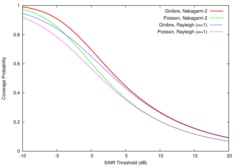
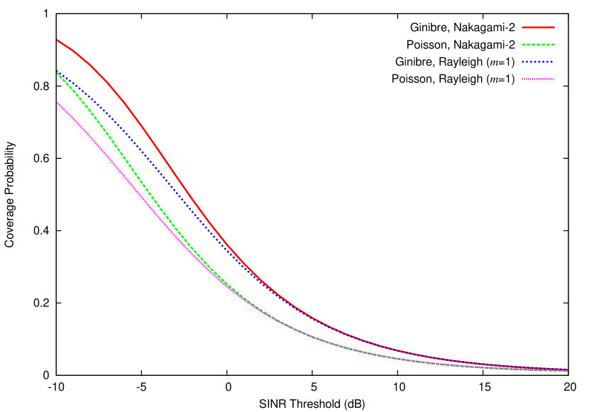
The results of some numerical experiments are presented. The first experiment is the comparison between the GPP and PPP based models. In Figure 1, the downlink coverage probability over Nakagami-$2$ fading is plotted for both the GPP and PPP based models, where two cases $\beta=1.25$ and $\beta=2.0$ (that is, $\ell(r)=r^{-2.5}$ and $\ell(r)=r^{-4}$) are computed. For comparison, the corresponding results over the Rayleigh fading, which are obtained in [5], are also displayed there. As in the Rayleigh fading case, the downlink coverage probability for the GPP based model dominates that for the PPP based model in the Nakagami-$m$ fading case. Furthermore, for both the GPP and PPP based models, the coverage probability seems asymptotically invariant in the value of $m$. This observation is, however, doubtful from the results of Lemma 1 and Theorem 2. Thus, this is further investigated in the next experiment.

Figure 1: Comparison of downlink coverage probability between the GPP and PPP based models for $\beta=1.25$ (top) and $\beta=2.0$ (bottom).

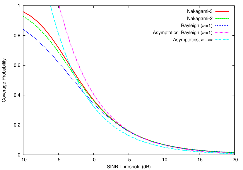
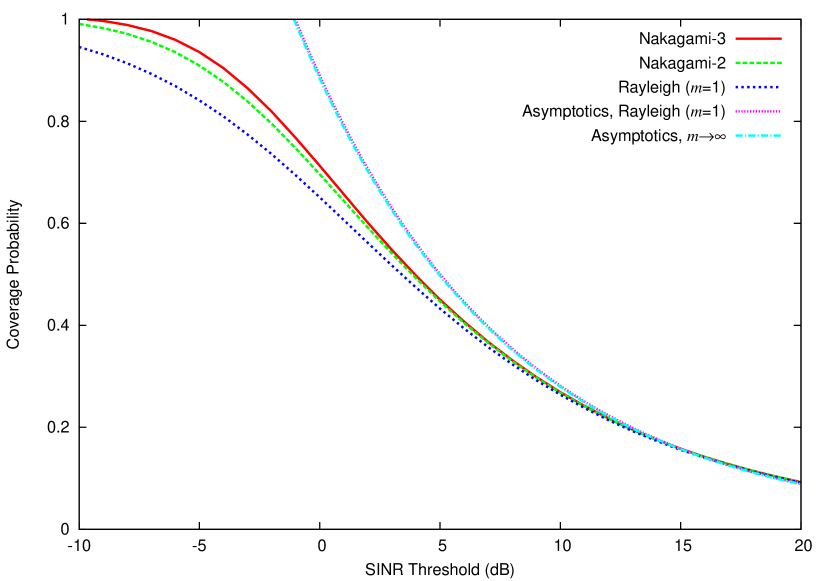
In the second experiment, we compare the downlink coverage probability in terms of $m$ of the Nakagami-$m$ fading. The coverage probability for $m=1$, $2$ and $3$ is plotted in Figure 2. The asymptotic results obtained in Proposition 2 and Theorem 2 are also drawn in the same figure, where the asymptotic constant $c^{(\infty)}$ for the case of $m\to\infty$ is estimated from 100 independent samples of $\bigl{(}\sum_{j=2}^{\infty}1/{Y_{j}}^{\beta}\bigr{)}^{-1/\beta}$ in (22). From the figure, indeed the downlink coverage probability seems increasing in $m=1$, $2$ and $3$. However, as $m\to\infty$, the asymptotic tail of the coverage probability is smaller than the others particularly for the value of $\beta$ close to $1$. This observation agrees with the results of Lemma 2 and Theorem 2. Anyway, a further investigation would be required concerning the impact of the value of $m$ of the Nakagami-$m$ fading.

Figure 2: Comparison of downlink coverage probability in terms of the value of $m$ for $\beta=1.25$ (top) and $\beta=2.0$ (bottom).

References

• [1] F. Baccelli and B. Błaszczyszyn, “Stochastic geometry and wireless networks, Volume I: Theory,” Foundations and Trends (R) in Networking, vol. 3, pp. 249–449, 2009.
• [2] ——, “Stochastic geometry and wireless networks, Volume II: Applications,” Foundations and Trends (R) in Networking, vol. 4, pp. 1–312, 2009.
• [3] M. Haenggi, Stochastic Geometry for Wireless networks.   Cambridge University Press, 2013.
• [4] S. Mukherjee, Analytical Modeling of Heterogeneous Cellular Networks: Geometry, Coverage, and Capacity.   Cambridge University Press, 2014.
• [5] N. Miyoshi and T. Shirai, “A cellular network model with Ginibre configured base stations,” Advances in Applied Probability, vol. 46, pp. 832–845, 2014.
• [6] G. L. Torrisi and E. Leonardi, “Large deviations of the interference in the Ginibre network model,” Stochastic Systems, vol. 4, pp. 1–33, 2014.
• [7] I. Nakata and N. Miyoshi, “Spatial stochastic models for analysis of heterogeneous cellular networks with repulsively deployed base stations,” Performance Evaluation, vol. 78, pp. 7–17, 2014.
• [8] N. Miyoshi and T. Shirai, “Cellular networks with α𝛼\alpha-Ginibre configurated base stations,” in The Impact of Applications on Mathematics: Proceedings of the Forum of Mathematics for Industry 2013.   Springer, 2014, pp. 211–226.
• [9] T. Kobayashi and N. Miyoshi, “Uplink cellular network models with Ginibre deployed base stations,” in 26th International Teletraffic Congress (ITC), 2014.
• [10] Y. Li, F. Baccelli, H. S. Dhillon, and J. G. Andrews, “Statistical modeling and probabilistic analysis of cellular networks with determinantal point processes,” 2014, arXiv:1412.2087 [cs.IT].
• [11] A. Soshnikov, “Determinantal random point fields,” Russian Mathematical Surveys, vol. 55, pp. 923–975, 2000.
• [12] T. Shirai and Y. Takahashi, “Random point fields associated with certain Fredholm determinants I: Fermion, Poisson and Boson processes,” Journal of Functional Analysis, vol. 205, pp. 414–463, 2003.
• [13] J. B. Hough, M. Krishnapur, Y. Peres, and B. Virág, Zeros of Gaussian Analytic Functions and Determinantal Point Processes.   American Mathematical Society, 2009.
• [14] S. Mukherjee, “Downlink SINR distribution in a heterogeneous cellular wireless network with max-SINR connectivity,” in 49th Annual Allerton Conference on Communication, Control and Computing, 2011, pp. 1649–1656.
• [15] P. Madhusudhanan, J. G. Restrepo, Y. Liu, and T. X. Brown, “Downlink coverage analysis in a heterogeneous cellular network,” in 2012 IEEE Global Communications Conference (GLOBECOM), 2012, pp. 4170–4175.
• [16] H. Keeler, B. Błaszczyszyn, and M. Karray, “SINR-based k𝑘k-coverage probability in cellular networks with arbitrary shadowing,” in 2013 IEEE International Symposium on Information Theory Proceedings (ISIT), 2013, pp. 1167–1171.
• [17] M. D. Renzo, A. Guidotti, and G. E. Corazza, “Average rate of downlink heterogeneous cellular networks over generalized fading channels: A stochastic geometry approach,” IEEE Transactions on Communications, vol. 61, pp. 3050–3071, 2013.
• [18] M. Nakagami, “The m𝑚m-distribution—A general formula of intensity distribution of rapid fading,” in Statistical Methods in Radio Wave Propagation: Proceedings of a Symposium Held at the University of California, Los Angeles, June 18–20, 1958, W. C. Hoffman, Ed.   Pergamon Press, 1960, pp. 3–36.
• [19] H. Huang, C. B. Papadias, and S. Venkatesan, MIMO Communication for Cellular Networks.   Springer, 2012.
• [20] H. S. Dhillon, M. Kountouris, and J. G. Andrews, “Downlink MIMO HetNets: Modeling, ordering results and performance analysis,” IEEE Transactions on Wireless Communications, vol. 12, pp. 5208–5222, 2013.
• [21] A. K. Gupta, H. S. Dhillon, S. Vishwanath, and J. G. Andrews, “Downlink coverage probability in MIMO HetNets with flexible cell selection,” in 2014 IEEE Global Communications Conference (GLOBECOM), 2014, pp. 1534–1539.
• [22] J. G. Andrews, F. Baccelli, and R. K. Ganti, “A tractable approach to coverage and rate in cellular networks,” IEEE Transactions on Communications, vol. 59, pp. 3122–3134, 2011.
• [23] A. Müller and D. Stoyan, Comparison Methods for Stochastic Models and Risks.   John Wiley & Sons, 2002.
• [24] E. Kostlan, “On the spectra of Gaussian matrices,” Linear Algebra and its Applications, vol. 162–164, pp. 385–388, 1992.
• [25] P. J. Olver, Applications of Lie Groups to Differential Equations.   Springer, 2000.
• [26] S. Roman, “The formula of Faà di Bruno,” American Mathematical Monthly, vol. 87, pp. 805–809, 1980.