A $(2+1)$-dimensional growth process with explicit stationary measures

Abstract.

We introduce a class of $(2+1)$-dimensional stochastic growth processes, that can be seen as irreversible random dynamics of discrete interfaces. “Irreversible” means that the interface has an average non-zero drift. Interface configurations correspond to height functions of dimer coverings of the infinite hexagonal or square lattice. The model can also be viewed as an interacting driven particle system and in the totally asymmetric case the dynamics corresponds to an infinite collection of mutually interacting Hammersley processes.

When the dynamical asymmetry parameter $(p-q)$ equals zero, the infinite-volume Gibbs measures $\pi_{\rho}$ (with given slope $\rho$) are stationary and reversible. When $p\neq q$, $\pi_{\rho}$ are not reversible any more but, remarkably, they are still stationary. In such stationary states, we find that the average height function at any given point $x$ grows linearly with time $t$ with a non-zero speed: $\mathbb{E}Q_{x}(t):=\mathbb{E}(h_{x}(t)-h_{x}(0))=V(\rho)t$ while the typical fluctuations of $Q_{x}(t)$ are smaller than any power of $t$ as $t\to\infty$.

In the totally asymmetric case of $p=0,q=1$ and on the hexagonal lattice, the dynamics coincides with the “anisotropic KPZ growth model” introduced by A. Borodin and P. L. Ferrari in [4, 5]. For a suitably chosen, “integrable”, initial condition (that is very far from the stationary state), they were able to determine the hydrodynamic limit and a CLT for interface fluctuations on scale $\sqrt{\log t}$, exploiting the fact that in that case certain space-time height correlations can be computed exactly. In the same setting they proved that, asymptotically for $t\to\infty$, the local statistics of height fluctuations tends to that of a Gibbs state (which led to the prediction that Gibbs states should be stationary).

2010 Mathematics Subject Classification: 82C20, 60J10, 60K35, 82C24
Keywords: Interface growth, Interacting particle system, Lozenge and domino tilings, Hammersley process, Anisotropic KPZ equation

1. Introduction

To motivate the object of our study, let us start with a well-known $(1+1)$-dimensional growth process. At all times $t$, the configuration is an integer-valued height function $x\in\mathbb{Z}\mapsto h_{x}(t)\in\mathbb{Z}$ with space increments $h_{x}-h_{x-1}=\pm 1$, see Fig. 1. Local minima turn to local maxima with rate $p$ (this corresponds to deposition of elementary squares) and local maxima to local minima with rate $q$ (evaporation of elementary squares). If positive interface gradients are identified with “particles” and negative gradients with “holes”, this process is equivalent to the one-dimensional Asymmetric Simple Exclusion process (ASEP).

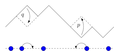
Figure 1. The ASEP: squares are deposed (i.e. minima turn to maxima) with rate $p$ and evaporate (i.e. maxima turn to minima) with rate $q$. In the particle interpretation, particles jump to the right/left with rate $q/p$ and cannot occupy the same site.

The study of this and similar stochastic growth processes in dimension $(1+1)$ witnessed a spectacular progress recently, especially in relation with the so-called KPZ equation, cf. e.g. [27, 16, 10] for recent reviews. Some of the basic questions that were solved for certain models include the identification of the translation-invariant stationary states (for ASEP, these are simply the combinations of Bernoulli measures for any intensity $\rho\in[0,1]$), the determination of the dynamic scaling exponents characterising the space-time correlation structure of height fluctuations, the study of the limit rescaled fluctuation process and its dependence on the type of initial condition. The same KPZ scaling relations appear also in the context of $(1+1)$-dimensional directed polymers in random environment, last passage percolation and random matrix theory, just to mention a few instances [27, 16, 10].

On the other hand, for $(d+1)$-dimensional stochastic growth models, $d\;\geqslant\;2$, the situation is much more rudimentary and mathematical results (see notably [26, 4]) are rare. In this work we introduce a $(2+1)$-dimensional stochastic growth process, for which we study the stationary measures and the corresponding large-time behavior of height fluctuations. The two-dimensional interfaces entering the definition of our process are discrete (i.e. heights are integer-valued) and are given by the height function associated to dimer coverings (perfect matchings) of either the infinite hexagonal or infinite square lattice [21]. Height functions corresponding to dimer coverings of bipartite planar graphs, or to the associated tilings of the plane, are classical examples of discrete two-dimensional interfaces. For instance, dimer coverings of the hexagonal lattice (i.e. tilings of the plane by lozenges of three different orientations) correspond to discrete monotone surfaces obtained by stacking unit cubes, see Figure 2. “Monotone” means that if we let $h_{x,y}$ denote the height w.r.t. the horizontal plane of the vertical column of cubes with horizontal coordinates $(x,y)$, then $h_{x,y}\;\geqslant\;\max(h_{x+1,y},h_{x,y+1})$. In a sense, discrete monotone height functions are the most natural $(2+1)$-dimensional analogue of the $(1+1)$-dimensional height functions appearing in the one-dimensional ASEP.

Given a density vector $\rho=(\rho_{1},\rho_{2},\rho_{3})\in\mathbb{R}_{+}^{3}$ with $\rho_{1}+\rho_{2}+\rho_{3}=1$, there exists [22] a unique infinite-volume translation-invariant ergodic Gibbs measure $\pi_{\rho}$ such that

• the three types of lozenges have densities $\rho_{i},i=1,2,3$ and

• conditioned on the tiling configuration outside a finite region $\Lambda$ of the plane, $\pi_{\rho}$ describes a uniformly random tiling of $\Lambda$.

The measures $\pi_{\rho}$ have an explicit determinantal structure that will play a role in this work and that is recalled in Section 2.2.

Figure 2. A lozenge tiling of a portion of the plane, or equivalently a monotone stacking of unit cubes

To model a growth process, we want to introduce a Markov evolution which is asymmetric or irreversible, in the sense that the interface has a net drift, proportional to an asymmetry parameter $p-q$. Moreover, as discussed in Section 1.1 below, in order that its fluctuations can be at least heuristically described by a $(2+1)$-dimensional KPZ-type equation, the average interface speed should be a non-linear function of the interface slope. The most natural $(2+1)$-dimensional generalization of the ASEP described above (but which is not the one we will study here) would be the following. Let

$$\Delta^{+}_{x,y}: =\min(h_{x-1,y},h_{x,y-1})-h_{x,y}\;\geqslant\;0$$ (1.1)

$$\Delta^{-}_{x,y}: =h_{x,y}-\max(h_{x+1,y},h_{x,y+1})\;\geqslant\;0,$$

and observe that $\Delta^{+}_{x,y}$ (resp. $\Delta^{-}_{x,y}$) is the maximal number of cubes we can add to (resp. remove from) column $(x,y)$ while respecting the condition $h_{x^{\prime},y^{\prime}}\;\geqslant\;\max(h_{x^{\prime}+1,y^{\prime}},h_{x^{\prime},y^{\prime}+1})$ for every $(x^{\prime},y^{\prime})$. For every column $(x,y)$, we add a single cube with rate $p$ if $\Delta^{+}_{x,y}>0$ and remove a single cube with rate $q$ if $\Delta^{-}_{x,y}>0$. In words, single elementary cubes are deposed (Fig. 4 top) with rate $p$ and removed (Fig. 4 bottom) with rate $q$ (compare with Fig. 1). We refer to this as the “single-flip dynamics”. If $p=q$ there is no drift and the infinite-volume Gibbs measures $\pi_{\rho}$ [22] are stationary and reversible. If instead $p\neq q$, the stationary states are not known, but they appear to be definitely very different from the equilibrium Gibbs measures [15, 32, 31]. This process has been studied numerically and one finds that typical interface fluctuations grow with time like $t^{\beta}$, with $\beta\simeq 0.24...$ [15, 32]. This is in sharp contrast with the ASEP, where the Bernoulli measures are stationary, irrespective of $p$ being equal or different from $q$. In the language of Section 1.1, the two-dimensional single-flip growth process is believed to belong to the so-called isotropic $(2+1)$-dimensional KPZ class when $q\neq p$. Unfortunately, the single-flip process is very hard to analyze mathematically and very little is known rigorously.

In this work we study, instead of the single-flip dynamics, a different $(2+1)$-dimensional irreversible growth process, that we call “bead dynamics” for reasons that will be clear later (in the hexagonal lattice case, “beads” or “particles” correspond to horizontal lozenges as in Fig. 2). As discussed in Section 1.1, the bead dynamics belongs (in contrast with the single-flip dynamics) to the so-called anisotropic $(2+1)$-dimensional KPZ class when $q\neq p$. Updates of the dynamics consist in adding or removing a random number $\;\geqslant\;1$ of cubes at some column $(x,y)$, in the following way (see Section 2.3 for a precise definition and Section 3.1 for the analogous construction on the square lattice). For every column $(x,y)$, we assign

• rate $p$ to the update $h_{x,y}\to h_{x,y}+i$ for every $i=1,\dots,\Delta^{+}_{x,y}$ (deposition of $i$ cubes to column $(x,y)$);

• rate $q$ to the update $h_{x,y}\to h_{x,y}-i$ for every $i=1,\dots,\Delta^{-}_{x,y}$ (removal of $i$ cubes from column $(x,y)$).

If $p=q$ again there is no drift and the measures $\pi_{\rho}$ [22] are stationary and reversible. Somewhat surprisingly, $\pi_{\rho}$ turns out to be stationary (but not reversible!) for any density vector $\rho$ and for any value of $p-q$. This is the content of our first result, Theorem 2.4. The same then clearly holds also if we add to the generator of the bead dynamics the generator of another process w.r.t. which $\pi_{\rho}$ is reversible. The measures $\pi_{\rho}$ and their convex combinations are the only stationary measures that can be obtained as $L\to\infty$ limits of stationary measures for the bead dynamics periodized on the torus of side $L$. In principle our result does not exclude the existence of other stationary measures that cannot be obtained this way; there might exist for instance analogs of the so-called “blocking measures” of one-dimensional asymmetric exclusion processes [13, 8].

We emphasize that it is a non-trivial fact that equilibrium Gibbs measures should remain stationary in presence of dynamical irreversibility. As we mentioned above, this is false for instance for the single-flip dynamics. Typically, one expects that a Gibbs measure of a reversible dynamics remains stationary after introduction of a drift only when the reversible dynamics satisfies a so-called “gradient condition” [30, 20, 2]. As we discuss in Section 4.1.1, for the symmetric dynamics with $p=q$ one can indeed identify a certain “gradient condition” that might help explain why Theorem 2.4 holds.

It is important to emphasize that stationarity of the Gibbs measures means that, if the process is started from the distribution $\pi_{\rho}$, the law of interface gradients is time-invariant. However, overall the height function has a time-dependent random shift $h_{x_{0}}(t)-h_{x_{0}}(0)$ where, say, $x_{0}$ is the origin of the plane. On average $h_{x_{0}}(t)-h_{x_{0}}(0)$ grows like $(p-q)t\,V$ for some non-zero and slope-dependent $V$ but the amplitude of its fluctuations cannot be deduced immediately from the stationary gradient measure $\pi_{\rho}$. Our second result, Theorem 3.1, says that the typical fluctuations of $h_{x}(t)-h_{x}(0)$ grow slower than any power of $t$. Under a certain (technical) restriction on the interface slope, we can actually prove that fluctuations are at most of order $\sqrt{\log t}$, which we believe to be the optimal order of magnitude. Recall that, in sharp contrast, for the single-flip dynamics fluctuations were observed numerically [15, 32] to grow like a non-trivial power of $t$.

A word about Theorem 2.4 (stationarity of $\pi_{\rho}$). Checking stationarity is easy for the process periodized on the torus of size $L$, see Section 4. The extension to the infinite lattice is, however, non-trivial. One may expect that, when $L$ is large, on local scales and for finite times the system does not feel the periodic boundary conditions and therefore locally the dynamics on the torus and on the infinite lattice could be coupled with high probability. The situation is however more subtle: while on the torus the process is always well-defined, in the infinite systems one can easily construct initial configurations such that, for instance, beads (horizontal lozenges) escape instantaneously to infinity. This is due to the fact that we allow for an unbounded amount of cubes to be deposed/removed at a time, since $\Delta^{\pm}_{x,y}$ is not bounded. In order for the coupling to work, one needs to prove that for typical initial conditions and with high probability, the random variables $\Delta^{\pm}_{x,y}$ remain sufficiently tight in time during the out-of-equilibrium evolution. An important ingredient in overcoming these difficulties is the work [28] by Seppäläinen on the one-dimensional Hammersley process [1, 28, 14]. In fact, viewing beads as particles, the bead dynamics can be seen as a two-dimensional generalization of the Hammersley process, or more precisely an infinite collection of interacting Hammersley processes, see Fig. 5 (a different two-dimensional generalization of the Hammersley process was introduced by Seppäläinen in [29]: in that case a full hydrodynamic limit was obtained, but the stationary measures and the size of height fluctuations remain unknown). As a side remark, the single-flip dynamics can be instead visualized in a natural way as an infinite collection of mutually interacting one-dimensional ASEPs, see caption of Fig. 5.

As we explain in some more detail in Section 3, in the totally asymmetric case $p=0,q=1$ and on the hexagonal lattice, the bead dynamics is the same as the interacting driven particle system introduced by A. Borodin and P. L. Ferrari in [4, 5]. In [4], for a specific, deterministic initial condition, the hydrodynamic limit and the convergence of height fluctuations on scale $\sqrt{\log t}$ to a Gaussian field were obtained. For such initial condition, the above-mentioned problem of proving that the dynamics is well-posed does not arise, simply because each bead has a deterministic, time-independent maximal position it can possibly reach, and therefore cannot escape to infinity. As we mention in Section 3, on the basis of [4, Prop. 3.2] it was natural to conjecture our Theorem 2.4.

1.1. Isotropic and anisotropic KPZ classes

In order to predict whether the fluctuations of a $(2+1)$-dimensional growth process should be described by a KPZ-type equation, one should look at the Hessian of $V$, the average interface velocity considered as a function of the interface slope. Indeed, the evolution of the fluctuations $h$ in the stationary state of slope $\nabla\phi$ should be governed on large space-time scales by a stochastic PDE of the type

$$\partial_{t}h=\nu\Delta h+Q(\partial_{x}h,\partial_{y}h)+\text{white noise},$$ (1.2)

with $\nu$ a diffusion coefficient and $Q(\cdot,\cdot)$ a quadratic form whose corresponding symmetric $2\times 2$ matrix is proportional to the Hessian of $V$ at $\nabla\phi$. (At present, it is not known how to regularize such equation in order to make it mathematically well-defined, as was done recently for its one-dimensional analog [18]).

The growth model is said to belong to the “anisotropic $(2+1)$-dimensional KPZ class” when the two eigenvalues of the quadratic form $Q$ have opposite sign, and to the “isotropic $(2+1)$-dimensional KPZ class” when they have the same sign. As discussed in [5], the bead dynamics belongs to the anisotropic class (the eigenvalues can be computed explicitly from formula (3.5) below for $V$).

Models in the anisotropic class are in a sense easier than those in the isotropic class. Indeed, in the former case it was predicted by Wolf [33] that the non-linearity $Q$ is irrelevant as far as the large-time behavior of the interface roughness is concerned, i.e. the fluctuations of $h_{x}(t)-h_{x}(0)$ should be of the same order $\sqrt{\log t}$ as for the linear Edwards-Wilkinson equation [12], where $Q$ is set to zero. Theorem 3.1 and Eq. (3.8) confirm this prediction, for the bead model. Apart from the bead dynamics we study here, there are a few other $(2+1)$-dimensional stochastic growth model models known to be in the anisotropic KPZ class, and all of them are exactly solvable in some sense. In this respect, let us mention the model introduced by Prähofer and Spohn in [26], for which height fluctuations are also known to grow like $\sqrt{\log t}$. See also [3, Sec. 3.3] for growth models in the same universality class: it would be interesting to see whether our result extend to these processes.

The situation is very different for models in the isotropic KPZ class. In this case there are, to our knowledge, no exactly solvable models and only numerical simulations are available (see [19] for an overview). The non-linearity $Q$ is expected to be relevant and to produce a non-trivial dynamical height fluctuation exponent. In particular, while neither the interface velocity $V$ nor the stationary states of the $(2+1)$-dimensional single-flip dynamics can be computed explicitly, the model is widely believed to belong to the isotropic KPZ class and, as mentioned above, the dynamical fluctuation exponent is numerically estimated to $\beta\simeq 0.24..$ [15, 32].

2. Irreversible lozenge dynamics and stationarity of Gibbs states

2.1. Configuration space

The Markov process we are interested in lives on $\Omega_{\mathcal{H}}$, the set of dimer coverings (perfect matchings) of the hexagonal lattice $\mathcal{H}$, or equivalently the set of lozenge tilings of the whole plane. See Figure 3.

Figure 3. A portion of dimer covering of $\mathcal{H}$ and the corresponding lozenge picture. The two beads in column $\ell$ are encircled and the vertices ${\rm b}_{0},{\rm w}_{0}$ are marked.

The “elementary moves” of the dynamics consist in rotating by an angle $\pi/3$ three dimers around a hexagonal face, see Figure 4.

Figure 4. The two elementary moves.

In this move, a horizontal dimer moves up or down a distance $1$. The generic move of the dynamics (defined precisely in Section 2.3), that was described in the introduction as the deposition/removal of $k$ cubes, can be seen as a concatenation of a random number $k\;\geqslant\;1$ of elementary moves in $k$ adjacent hexagons in the same vertical column. We can therefore see each “horizontal dimer/lozenge” (we call them “beads” hereafter) as attached to a “column” (an infinite vertical stack of hexagons): the bead can move up and down along the column but not change column. The set of possible bead positions can be identified with $\mathbb{Z}$ on, say, even columns and with $\mathbb{Z}+1/2$ on odd columns. Note that beads of neighboring columns are interlaced: if on column $\ell$ there are two beads at positions $z_{1}<z_{2}$ then necessarily in column $\ell-1$ there is a bead at a position $z_{1}<z_{3}<z_{2}$ and similarly for column $\ell+1$.

Definition 2.1.

For each dimer configuration $\sigma$ and bead $b$ we let $I^{+}_{b}=I^{+}_{b}(\sigma)$ be the collection of available positions above it, i.e. positions that $b$ can reach via a concatenation of elementary moves that do not touch any other bead and do not violate the interlacing constraints. We define similarly $I^{-}_{b}=I^{-}_{b}(\sigma)$ as the collection of available positions below it.

Remark 2.2.

Given a finite or infinite subset $\Lambda$ of $\mathcal{H}$, we denote $\sigma|_{\Lambda}$ the dimer configuration restricted to $\Lambda$ and $\eta|_{\Lambda}$ the configuration of beads restricted to $\Lambda$. If $\Lambda=\mathcal{H}$ we omit the index $\Lambda$. If (as will be the case in Theorem 2.4 below) every column contains at least one bead, $\sigma$ can be reconstructed by knowing just $\eta$. In this case we will identify a dimer covering with a bead configuration.

2.2. Height function

On $\mathcal{H}$, we take a coordinate frame where the axis $\vec{e}_{1}$ forms a clockwise angle $+5\pi/6$ with the usual horizontal axis and the axis $\vec{e}_{2}$ an angle $+\pi/6$, see Figure 3. We also set $\vec{e}_{3}=-\vec{e}_{1}-\vec{e}_{2}$ to be the vertical unit vector.

Definition 2.3.

Let $\mathcal{H}^{*}$ denote the dual graph of $\mathcal{H}$ (it is a triangular lattice, whose vertices are vertices of lozenges). Vertices of $\mathcal{H}^{*}$ are as usual identified with hexagonal faces of $\mathcal{H}$.

The height function $h:\mathcal{H}^{*}\mapsto\mathbb{Z}$ is an integer-valued function, defined up to an arbitrary additive constant. When moving one step in the $\vec{e}_{1}$ or $\vec{e}_{2}$ direction, the height increases by $1$ when a dimer (or equivalently lozenge) is crossed and stays constant otherwise.

Note that, with this convention, $h$ corresponds to minus the height function with respect to the horizontal plane, and observe also that when moving one step in the $\vec{e}_{3}$ direction, $h$ decreases by $1$ if no dimer is crossed and stays constant otherwise.

Given ${\rho}=(\rho_{1},\rho_{2})\in\mathbb{R}^{2}$ with $0<\rho_{1},\rho_{2}<1$, and $0<\rho_{1}+\rho_{2}<1$ (we call ${\rho}$ a non-extremal slope) there exists a unique translation-invariant ergodic Gibbs state $\pi_{{\rho}}$ with slope $\rho$. This is a translation invariant probability law on the set of dimer coverings of $\mathcal{H}$, that satisfies (cf. [21, Sec. 6]):

• $\pi_{{\rho}}$ is ergodic with respect to translations by $a\vec{e}_{1}+b\vec{e}_{2},a,b\in\mathbb{Z}$;

• it satisfies the Dobrushin-Lanford-Ruelle equations: conditionally on the dimer configuration $\sigma_{\mathcal{G}^{c}}$ outside a given finite subset $\mathcal{G}\subset\mathcal{H}$, $\pi_{{\rho}}$ is the uniform measure over all dimer coverings $\sigma_{\mathcal{G}}$ of $\mathcal{G}$ compatible with $\sigma_{\mathcal{G}^{c}}$, i.e. such that $\sigma_{\mathcal{G}^{c}}\cup\sigma_{\mathcal{G}}$ is a dimer covering of $\mathcal{H}$;

• it has slope $\rho$, i.e. $\pi_{{\rho}}(h_{x+\vec{e}_{i}}-h_{x})=\rho_{i},i=1,2$.

Note that $\rho_{1}$ is the density of south-east oriented lozenges, $\rho_{2}$ is the density of north-east lozenges and $\rho_{3}:=1-\rho_{1}-\rho_{2}$ the density of horizontal lozenges. The non-extremality requirement on ${\rho}$ means that all three types of lozenges have non-zero density.

The measure $\pi_{\rho}$ is in a sense completely known and has a determinantal representation, that we recall here briefly (cf. in particular (2.3)), since it will be needed in the following. See [22, 21] for further details. First of all, color sites of $\mathcal{H}$ white/black according to whether they are the left/right endpoint of a horizontal edge and let $\mathcal{H}_{W},\mathcal{H}_{B}$ be the sub-lattice of white/black vertices. We denote ${\rm w}_{0},{\rm b}_{0}$ the black/white vertices indicated in Figure 3 and we let ${\rm w}_{x},{\rm b}_{x}$, with $x=(x_{1},x_{2})\in\mathbb{Z}^{2}$, be the translation of ${\rm w}_{0},{\rm b}_{0}$ by $x_{1}\vec{e}_{1}+x_{2}\vec{e}_{2}$.

Take a triangle with angles $\theta_{i}=\pi\rho_{i},i=1,2,3$ and let $k_{i},i=1,2,3$ be the length of the side opposite to $\theta_{i}$. Define the Kasteleyn matrix $K=\{K({\rm b},{\rm w})\}_{{\rm b}\in\mathcal{H}_{B},{\rm w}\in\mathcal{H}_{W}}$ as follows: If ${\rm b},{\rm w}$ are not nearest neighbors, then $K({\rm b},{\rm w})=0$. If they are nearest neighbors, then $K({\rm b},{\rm w})=k_{1}$ or $k_{2}$ or $k_{3}$ according to whether the edge ${\rm b}{\rm w}$ is oriented south-east, north-east or horizontal.

Define also the matrix $K^{-1}=\{K^{-1}({\rm w},{\rm b})\}_{{\rm w}\in\mathcal{H}_{W},{\rm b}\in\mathcal{H}_{B}}$ as

$$K^{-1}({\rm w}_{x},{\rm b}_{x^{\prime}})=\frac{1}{(2\pi i)^{2}}\int_{\mathbb{T}}\frac{z^{-(x^{\prime}_{2}-x_{2})}w^{x_{1}^{\prime}-x_{1}}}{P(z,w)}\frac{dz}{z}\frac{dw}{w}:=\frac{1}{(2\pi i)^{2}}\int_{\mathbb{T}}\frac{z^{-(x^{\prime}_{2}-x_{2})}w^{x_{1}^{\prime}-x_{1}}}{k_{3}+k_{1}z+k_{2}w}\frac{dz}{z}\frac{dw}{w}$$ (2.1)

where the integral is taken over the two-dimensional unit torus $\mathbb{T}:=\{(z,w)\in\mathbb{C}^{2}:|z|=|w|=1\}$. The long-distance behavior of $K^{-1}$ is precisely known [22]: since the polynomial $P$ has two simple zeros on the torus, $K^{-1}$ decays like the inverse of the distance so that in particular

$$|K^{-1}({\rm w}_{0},{\rm b}_{x})|\;\leqslant\;\frac{C(\rho)}{|x_{1}|+|x_{2}|+1}$$ (2.2)

with $C(\rho)<\infty$ (this in general fails if $\rho$ is extremal, e.g. if only one of the three dimer orientations has positive density).

Given a set of (not necessarily horizontal) edges $e_{1}=({\rm w}_{1},{\rm b}_{1}),\dots,e_{k}=({\rm w}_{k},{\rm b}_{k})$ of $\mathcal{H}$, the correlation function $\pi_{\rho}(\delta_{e_{1}}\dots\delta_{e_{k}})$ (with $\delta_{e}$ the indicator function that there is a dimer at $e$) is given by

$$\pi_{\rho}(\delta_{e_{1}}\dots\delta_{e_{k}})=\left(\prod_{i=1}^{k}K({\rm b}_{i},{\rm w}_{i})\right)\det\left(K^{-1}({\rm w}_{i},{\rm b}_{j})\right)_{1\;\leqslant\;i,j\;\leqslant\;k}.$$ (2.3)

Note, also in view of formula (2.1), that the r.h.s. of (2.3) is invariant if we multiply all $k_{i}$ by a common factor $c$, so that we may for instance fix the sum $k_{1}+k_{2}+k_{3}$ to $1$.

2.3. Definition of the dynamics and stationarity of Gibbs states

The dynamics is informally defined as follows (cf. Fig. 5). To each column $\ell$ and to each possible bead position $z$ (horizontal edge of $\mathcal{H}$) we associate two independent Poisson clocks of mean $p\in[0,1]$ and $q\in[0,1]$ respectively. We call them $p$-clocks and $q$-clocks, with obvious meaning. Clocks at different locations are independent. When a $p$-clock (resp. a $q$-clock) at $(\ell,z)$ rings, if $(\ell,z)$ is occupied by a bead we do nothing. Otherwise, we look at the highest (resp. lowest) bead (if any) on column $\ell$ that is at position lower (resp. higher) than $z$: if it can be moved to $z$ without violating the interlacing constraints then we do so, otherwise we do nothing.

Figure 5. A portion of the lattice with the allowed moves and the respective rates. Beads are drawn as black lozenges. When $p=1,q=0$ or $p=0,q=1$ the process can be seen as an infinite set of discrete Hammersley processes, one per column, each interacting with the two neighboring processes. If instead we allowed particles to jump only by $\pm 1$ with rates $p/q$, the process would be the single-flip dynamics described in the introduction and would correspond to an infinite collection of mutually interacting asymmetric simple exclusion processes (ASEP), one per column.

It is not obvious that the process is well defined on the infinite lattice. The danger is that beads could escape to $+\infty$ or to $-\infty$ in finite time (even in an arbitrarily small time). This may occur when spacings between beads in the initial configuration grow sufficiently fast at infinity. The problem is that the rate at which a bead moves, say, upward is $p\times|I^{+}_{b}|$ and the average size of the jump is $(|I^{+}_{b}|+1)/2$, and $|I^{+}_{b}|$ is not bounded.

Our first result (Theorem 2.4) is that the process is well defined for almost every initial condition sampled from $\pi_{{\rho}}$ and that $\pi_{{\rho}}$ is invariant. “Well-defined” means that the displacement of every bead with respect to its position at time zero is almost surely finite for every $t\;\geqslant\;0$. In the symmetric case $p=q$, assuming that the process is well defined, invariance of the Gibbs measure is obvious because it is reversible.

To precisely formulate the result, let us start by defining, given $K=(K_{p},K_{q})\in(\mathbb{R}^{+})^{2}$, a cut-off process where $p$-clocks at distance more than $K_{p}$ (resp. $q$-clocks at distance more than $K_{q}$) from the origin of $\mathcal{H}$ are switched off. As long as $K_{p},K_{q}<\infty$ there is no problem in defining the process on the whole $\mathcal{H}$, since this is effectively a Markov jump process on a finite state space (once a particle is inside the ball of radius $\max(K_{q},K_{p})$ it cannot leave it and therefore there is only a finite number of particles, determined by the initial condition, that can ever move). We call $X^{\sigma}_{t;K}$ the configuration at time $t$, started from initial condition $\sigma$. Given a column $\ell$, let $z_{t}(\ell,n;K)$ be the position of its $n^{th}$ bead at time $t$, with $z_{t}(\ell,n;K)<z_{t}(\ell,n+1;K)$. The label $n$ is assigned in the initial condition and is attached to beads forever. For instance, one can assign the label $(\ell,0)$ to the lowest bead in $\ell$ with non-negative vertical coordinate (in the initial condition). We assume hereafter that in each column there is a doubly infinite set of beads, i.e. the index $n$ runs over all of $\mathbb{Z}$.

Two processes with different cut-offs $K$ and $K^{\prime}$ can be coupled in the obvious way: their $p$-clocks (resp. $q$-clocks) are the same in the ball of radius $\min(K_{p},K^{\prime}_{p})$ (resp. $\min(K_{q},K^{\prime}_{q})$). It is then easy to check that $z_{t}(\ell,n;K)$ is increasing w.r.t. $K_{p}$ and decreasing w.r.t. $K_{q}$. We will then define

$$z_{t}(\ell,n)=\lim_{K_{q}\to\infty}\lim_{K_{p}\to\infty}z_{t}(\ell,n;K)$$ (2.4)

to be the position of the $(\ell,n)$-th bead at time $t$ for the process without cut-off.

Assuming that $z_{t}(\ell,n)$ is finite for every $(\ell,n)$, call $X_{t}$ the corresponding bead configuration and let $\mathbb{P}_{\nu}$ be the law of the process $(X_{t})_{t\;\geqslant\;0}$ started with initial distribution $\nu$ (if $\nu$ is concentrated at some $\sigma$, then we write just $\mathbb{P}_{\sigma}$).

Theorem 2.4.

For almost every initial condition sampled from $\pi_{{\rho}}$, with ${\rho}$ a non-extremal slope, the limit (2.4) is almost surely finite for all $(\ell,n)$ and $t\;\geqslant\;0$. Moreover, $\pi_{{\rho}}$ is invariant. More precisely, if $f$ is a local bounded function of the dimer configuration one has for every $t\;\geqslant\;0$

$$\mathbb{E}_{\pi_{\rho}}(f(X_{t}))=\int\pi_{{\rho}}(d\sigma)\mathbb{E}_{\sigma}f(X_{t})=\pi_{{\rho}}(f).$$ (2.5)

Here, a function $f$ is said to be local if it depends only on $\sigma_{\Lambda}$ for some finite $\Lambda$. It is also possible to see (cf. Remark 7.7) that the limit (2.4) does not depend on the order how one takes the limits $\lim_{K_{q}\to\infty}$ and $\lim_{K_{p}\to\infty}$.

Theorem 2.4 is proven partly in Section 6 (existence of the dynamics) and partly in Section 8.1 (invariance of $\pi_{\rho}$).

Remark 2.5.

With this result in hand, it is clear that one can construct many other driven processes that leave $\pi_{\rho}$ invariant, simply adding to the generator of the bead dynamics another generator $\mathcal{L}$ with respect to which $\pi_{\rho}$ is reversible (for instance, $\mathcal{L}$ could be the generator of the single-flip dynamics with symmetric rates).

It is a relatively standard fact to deduce from Theorem 2.4 that, if we start from $\pi_{\rho}$ conditioned to have a bead say at the origin, then the law of the dimer configuration re-centered at the time-evolving position of this marked bead (tagged particle) is time-independent, see Section 8.2. More precisely, fix a horizontal edge $e_{0}$ of $\mathcal{H}$. Given an initial condition $\sigma$ such that there is a bead at $e_{0}$, call $\phi_{t}$ its vertical coordinate at time $t$ (the horizontal coordinate does not change). Let also $\hat{X}_{t}:=\tau_{\phi_{t}-\phi_{0}}X_{t}$, with $\tau_{x}$ the vertical translation by $x\in\mathbb{Z}$, be the dimer configuration viewed from the tagged bead and call $\hat{\mathbb{P}}_{\nu}$ the law of the process $(\hat{X}_{t})_{t\;\geqslant\;0}$ started from some initial distribution $\nu$. Finally, let $\hat{\pi}_{\rho}$ be the Gibbs measure $\pi_{\rho}$ conditioned on the event that there is a bead at $e_{0}$.

Proposition 2.6.

The measure $\hat{\pi}_{\rho}$ is invariant for the dynamics of the dimer configuration viewed from the tagged bead: for every bounded local function $f$ and $t\;\geqslant\;0$,

$$\hat{\pi}_{\rho}(f(\hat{X}_{t}))=\hat{\pi}_{\rho}(f).$$ (2.6)

3. Interface speed and fluctuations

The stationary states $\pi_{\rho}$ are characterized by an upward or downward flux of beads, according to whether $p>q$ or $p<q$. The particle flux is directly related to the average height increase in the stationary state. While the height function was defined only up to an additive constant, one can define unambiguously the increase of the height at a face $x$ from time $0$ to $t$: $Q_{x}(t):=h_{x}(t)-h_{x}(0)$ equals the number of beads that cross the face $x$ downward up to time $t$, minus the number of beads that cross it upward.

For each horizontal bond $e$ let $b^{+}(e)$ (resp. $b^{-}(e)$) be the lowest (resp. highest) bead in the column of $e$, at vertical position strictly higher (resp. strictly lower) than $e$. Also, call $V(e,\uparrow)$ the collection of hexagons that $b^{-}(e)$ has to cross to reach position $e$ and set $V(e,\uparrow)=\emptyset$ if this move is not possible (keeping the other beads where they are). Define $V(e,\downarrow)$ similarly.

The following result identifies the average height drift and shows that the fluctuations of $Q_{x}(t)$ in the stationary measure are smaller than any power of $t$:

Theorem 3.1.

For any face $x$,

$$\mathbb{E}_{\pi_{\rho}}(Q_{x}(t))=t\,(q-p)\,J$$ (3.1)

with

$$J=\pi_{\rho}(|\{e:x\in V(e,\uparrow)\}|)>0.$$ (3.2)

For every $\delta>0$,

$$\lim_{t\to\infty}\mathbb{P}_{\pi_{\rho}}(|Q_{x}(t)-\mathbb{E}_{\pi_{\rho}}(Q_{x}(t))|\;\geqslant\;t^{\delta})=0.$$ (3.3)

Note that only edges $e$ in the same column as $x$ and above it can contribute to $J$. The value of $J$ is independent of $x$ by translation invariance of $\pi_{\rho}$. The r.h.s. of (3.1) is linear in $t$ because of stationarity of $\pi_{\rho}$ and linear in $(q-p)$ because the stationary state $\pi_{\rho}$ does not depend on $p,q$.

Theorem 3.1 is proven in Section 9.

It is not obvious to compute $J$ explicitly in terms of the slope $\rho$, starting directly from the determinantal representation of the Gibbs states. In [4, 5], A. Borodin and P. L. Ferrari considered the dynamics for $p=0,q=1$ for a special, “integrable”, initial condition $\omega$, whose height function $(h_{0}(x))_{x\in\mathcal{H}^{*}}$ is deterministic and has non-constant slope (see Fig. 1.2 of [4]: lozenges with a dot correspond to our south-east oriented lozenges, white squares to our north-east lozenges, while dark lozenges correspond to our beads). Let us emphasize that with such initial condition, each bead has a deterministic lowest position it can possibly reach on its column (this is related to the fact that in [4, Fig. 1.1, 1.2] there is no dotted lozenge with coordinate $n<0$), so that the well-posedness of the process poses no problem in that case. One of the results of [4] is a hydrodynamic limit, that in our notations we can formulate as follows: for every $\xi,\eta$ and $\tau>0$ one has

$$\lim_{L\to\infty}\frac{1}{L}\mathbb{E}_{\omega}\left[h_{(\lfloor\xi L\rfloor,\lfloor\eta L\rfloor)}(\tau L)\right]={\bf h}(\xi,\eta,\tau)$$ (3.4)

and ${\bf h}$ satisfies

$$\partial_{\tau}{\bf h}=V(\partial_{\xi}{\bf h},\partial_{\eta}{\bf h})=\frac{1}{\pi}\frac{\sin(\pi\partial_{\eta}{\bf h})\sin(\pi\partial_{\xi}{\bf h})}{\sin(\pi(\partial_{\eta}{\bf h}+\partial_{\xi}{\bf h}))}$$ (3.5)

(this corresponds to formulas (1.9)-(1.11) in [4], after after a suitable change of coordinates due to the fact that in [4, 5] the height is not taken with respect to the horizontal plane and a different reference frame than our $\vec{e}_{1},\vec{e}_{2}$ frame is used). From this, one can naturally guess that $J$ in (3.2) should be given by

$$J=\frac{1}{\pi}\frac{\sin(\pi\rho_{1})\sin(\pi\rho_{2})}{\sin(\pi(\rho_{1}+\rho_{2}))}.$$ (3.6)

Since $\rho_{1},\rho_{2}$ and $\rho_{1}+\rho_{2}$ are in $(0,1)$, the above expression is immediately seen to be positive. After a first version of this work was completed, Chhita and Ferrari [9] proved, through a smart combinatorial identity based on the determinantal structure of the Gibbs states, that indeed (3.6) holds.

By the way, Proposition 3.2 of [4] says that the law of local dimer observables around point $(\lfloor\xi L\rfloor,\lfloor\eta L\rfloor)$ at time $\tau L$ tends as $L\to\infty$ to that of the same observables under the Gibbs state of slope $\rho=(\partial_{\xi}{\bf h}(\xi,\eta,\tau),\partial_{\eta}{\bf h}(\xi,\eta,\tau))$. On the basis of this, it was natural to conjecture that our Theorem 2.4 holds.

Referring to (3.3), we believe that the order of magnitude of the variance of $Q_{x}(t)$ is actually $\log t$: this is indeed the result found by Borodin and Ferrari [4, 5], in the particular case where $p=0$, $q=1$ and for the special initial condition $\omega$ mentioned above. In this respect, our method allows indeed to refine estimate (3.3), under a (purely technical, we believe) condition on the slope $\rho$, to the following:

Theorem 3.2.

If the slope $\rho$ satisfies

$$\sqrt{k_{1}k_{2}}C(\rho)<1,$$ (3.7)

with $C(\rho)$ defined in (A.25) and $k_{1},k_{2}$ as in (2.1), we have for some $c<\infty$

$$\limsup_{t\to\infty}\mathbb{P}_{\pi_{\rho}}(|Q_{x}(t)-\mathbb{E}_{\pi_{\rho}}(Q_{x}(t))|\;\geqslant\;u\sqrt{\log t})\;\leqslant\;\frac{c}{u^{2}}.$$ (3.8)

For instance, if $\rho=(1/3,1/3)$ (the three types of dimers have density $1/3$, in which case $k_{1},k_{2},k_{3}$ are all equal) one finds, evaluating numerically the integral in (A.25), that the l.h.s. of (3.7) is $0.896...<1$, so that (3.8) holds. By continuity, this remains true in a whole neighborhood of $\rho=(1/3,1/3)$ while, again numerically, (3.7) does not seem to be satisfied in the whole set of non-extremal slopes $\rho$.

Let us stress once more that we believe (3.8) to hold for every non-extremal $\rho$ and to be of the optimal order w.r.t. $t$, while we do not attach any particular meaning to condition (3.7).

Remark 3.3.

It is possible to define alternatively the stationary drift as follows. Sample $\sigma$ from $\hat{\pi}_{{\rho}}$ and call as above $\phi_{t}$ the vertical coordinate of the tagged bead $b_{0}$ at time $t$. From Proposition 2.6 it is easy to deduce that the average of $\phi_{t}-\phi_{0}$ is exactly linear in $t$, while from the definition of the process and the fact that $|I^{-}_{b_{0}}|$ has the same law as $|I^{+}_{b_{0}}|$ (the Gibbs measures are invariant by reflection through the center of any given hexagonal face; this follows e.g. from uniqueness of $\pi_{\rho}$ given the slope) one sees

$$v:=\frac{1}{t}\int\hat{\pi}_{\rho}(d\sigma)\mathbb{E}_{\sigma}(\phi_{t}-\phi_{0})=(p-q)\hat{\pi}_{\rho}(|I^{+}_{b_{0}}|(|I^{+}_{b_{0}}|+1)/2).$$ (3.9)

It is not hard to deduce from the stationarity of $\pi_{\rho}$ that

$$\mathbb{E}_{\pi_{\rho}}(h_{x}(t)-h_{x}(0))=-t\,\rho_{3}\,v,$$ (3.10)

where we recall that $\rho_{3}$ is the density of beads (the reason for the minus sign is that when a bead moves upward the height function decreases). Indeed, suppose for simplicity that $p=1,q=0$. The l.h.s. of (3.10) equals minus the sum over the the edges $e$ below $x$ of the probability that there is a bead at $e$ at time zero and that at time $t$ is has moved at least $n+1$ steps up, with $n\;\geqslant\;0$ the number of hexagonal faces between $e$ and $x$. By translation invariance of $\pi_{\rho}$, this equals

$$-\rho_{3}\sum_{n\;\geqslant\;0}\int\hat{\pi}_{\rho}(d\sigma)\mathbb{P}_{\sigma}(\phi_{t}-\phi_{0}>n)=-\rho_{3}\int\hat{\pi}_{\rho}(d\sigma)\mathbb{E}_{\sigma}(\phi_{t}-\phi_{0})=-t\,\rho_{3}\,v$$ (3.11)

where we used positivity of $\phi_{t}-\phi_{0}$ in the first equality and (3.9) in the second.

3.1. Extension to dominos (perfect matchings of $\mathbb{Z}^{2}$)

Our result extends to perfect matchings of $\mathbb{Z}^{2}$, or equivalently domino tilings of the plane, cf. Fig. 6: also in this case, one can define an asymmetric Markov dynamics (the height function has a non-zero drift) that leaves the Gibbs states invariant. We give only a sketchy description of the generalization, omitting those details that are identical to the case of the honeycomb lattice.

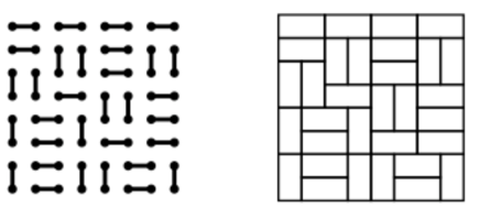
Figure 6. The correspondence between dimer covering (perfect matching) of $\mathbb{Z}^{2}$ and domino tiling of the plane.

Since $\mathbb{Z}^{2}$ is bipartite we can color its vertices black/white with the rule that each vertex has neighbors only of the opposite color. The height function $h$ on the set of faces of $\mathbb{Z}^{2}$ can be defined (modulo an arbitrary additive constant) as follows: for each $x,y$ choose any nearest-neighbor path $C_{x\to y}$ from $x$ to $y$ and set

$$h_{y}-h_{x}=\sum_{e\in C_{x\to y}}\sigma_{e}(\delta_{e}-1/4)$$ (3.12)

with the sum running over the edges crossed by the path, $\sigma_{e}=\pm 1$ according to whether $C_{x\to y}$ crosses $e$ with the white vertex on the left/right and $\delta_{e}$ the indicator function that there is a dimer at $e$. The definition is independent of the choice of path.

The classification of translation-invariant ergodic Gibbs states is analogue to the honeycomb lattice case (actually the structure is the same for all planar, periodic, infinite bipartite graphs [22]): there exists an open polygon $P\subset\mathbb{R}^{2}$ (for the lattice $\mathbb{Z}^{2}$ it is a square, while for $\mathcal{H}$ it is a triangle, as discussed in Section 2.2) such that for every $\rho=(\rho_{1},\rho_{2})\in P$ (non-extremal slope) there exists a unique translation-invariant ergodic Gibbs state $\pi_{\rho}$ satisfying

$$\pi_{\rho}(h_{x+\vec{e}_{i}}-h_{x})=\rho_{i},\;i=1,2,$$ (3.13)

where the vectors $\vec{e}_{i}$ are as in Figure 7. The determinantal representation (2.3) still holds, with a different polynomial $P(z,w)$ that however still has two simple zeros on the torus $\mathbb{T}$. In order to define the irreversible dynamics that leaves the Gibbs states invariant, we have to find an analogue of the “columns” and “beads”. This is inspired by [24, 23]. The set of square faces of $\mathbb{Z}^{2}$ is sub-divided into infinite “columns” (indexed by $\ell\in\mathbb{Z}$), i.e. diagonally oriented zig-zag paths, see Figure 7. Dimers that occupy an edge across a column are called “beads”. Each column is oriented along the positive $\vec{e}_{1}$ direction, so it makes sense to say that a bead $b_{1}$ in column $\ell$ is above a bead $b_{2}$ in the same column.

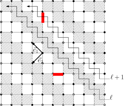
Figure 7. A portion of $\mathbb{Z}^{2}$ with vertices colored black/white. The colored graph is periodic, i.e. invariant w.r.t. translations by $n_{1}\vec{e}_{1}+n_{2}\vec{e}_{2},n_{1},n_{2}\in\mathbb{N}$. The white and shaded zig-zag regions are the “columns”, indexed by $\ell$. Columns are oriented in the positive $\vec{e}_{1}$ direction. The two thick bonds, transversal to columns, represent two beads.

Given columns $\ell,\ell+1$, call $Y_{\ell}$ the set of vertices of $\mathbb{Z}^{2}$ shared by the two columns and order the sites of $Y_{\ell}$ according their $\vec{e}_{1}$ coordinate. Then, a bead $b$ on column $\ell$ is said to be higher than a bead $b^{\prime}$ on $\ell+1$ if the vertex of $b$ on $Y_{\ell}$ is higher than the vertex of $b^{\prime}$ on $Y_{\ell}$. With this definition, it is easy to see that beads satisfy the same interlacement property as on the honeycomb graph: given beads $b_{1},b_{2}$ on $\ell$, there exists $b_{3}$ on $\ell-1$ and $b_{4}$ on $\ell+1$ with $b_{1}<b_{3}<b_{2}$ and $b_{1}<b_{4}<b_{2}$. Also, like on the honeycomb lattice, it is easy to see that if there is at least a bead in each column, then it is possible to reconstruct the whole dimer covering knowing only the bead positions.

The dynamics is then defined as follows. Assign to any possible bead position, i.e. to each edge that is transversal to some column, two independent Poisson clocks of rates $p$ and $q$, as before. All clocks are independent. When a $p$-clock (resp. $q$-clock) at edge $e$ of column $\ell$ rings, if there is a bead at $e$ then do nothing. Otherwise, move the first bead below (resp. above) $e$ in column $\ell$ to position $e$, provided this does not violate the interlacing constraints. Note that the dynamics is the same as on the honeycomb lattice, only the definition of “column” and “bead” being lattice-dependent. Observe also that each move can be seen as a concatenation of elementary moves on $n$ adjacent faces along the same column, each elementary move consisting in the rotation by $\pi/2$ of two dimers on the same face of $\mathbb{Z}^{2}$ (Fig. 8).

Figure 8. The two elementary moves of the domino dynamics

In fact, the effect of an elementary move is to shift a single bead one position up or down along its column. Note that, like in the case of the hexagonal lattice, when a bead moves one step upward crossing a face $f$, the height function at $f$ changes by $-1$.

As in Section 3, given an edge $e$ transversal to some column $\ell$, call $b^{-}(e)$ the highest bead in $\ell$, strictly lower than $e$ and let $V(e,\uparrow)$ the collection of square faces of $\ell$ that $b^{-}(e)$ crosses when it is moved to $e$ (with $V(e,\uparrow)=\emptyset$ if the move is not allowed). Then:

Theorem 3.4.

The claim of Theorems 2.4 and 3.1 hold also for the bead dynamics on dimer coverings of $\mathbb{Z}^{2}$.

With the exception of Section 4.2, in the rest of the work we will always consider the case of the hexagonal lattice.

4. Dynamics on the torus

4.1. Honeycomb lattice

We will let the torus $\mathbb{T}_{L}$ denote the hexagonal graph $\mathcal{H}$, periodized (with period $L$) along directions $\vec{e}_{2},\vec{e}_{3}$ and we assume that $L\;\geqslant\;3$. Note that now columns $\ell$ along which beads move are $L$ “circles” containing $L$ hexagonal faces. We will say as before that a bead moves “upward” or “downward”, but what we mean is that it moves in the positive or negative $\vec{e}_{3}$ direction around the torus.

Let $N^{L}_{{\rho}}$ be the set of configurations such that the height changes by $\lfloor\rho_{2}L\rfloor$ (resp. $\lfloor L\rho_{3}\rfloor-L$) along any closed path winding once in the positive $\vec{e}_{2}$ (resp. $\vec{e}_{3}$) direction. On each column $\ell$ there are $\lfloor\rho_{3}L\rfloor$ beads and bead positions on neighboring columns are again interlaced. We denote $\pi^{L}_{{\rho}}$ the uniform measure over $N^{L}_{{\rho}}$. It is known that $\pi^{L}_{{\rho}}$ converges weakly to $\pi_{{\rho}}$, if the configuration space is equipped with the product topology [22]. Essentially, averages of bounded local functions converge.

On $\mathbb{T}_{L}$ the process is defined similarly as in Section 2.3 for the infinite graph. For instance, when a $p$-clock at an edge $e$ rings, one moves to $e$ the first bead that is found when proceeding in the $-\vec{e}_{3}$ direction from $e$ along the same column, unless this move is forbidden by the interlacing constraint. The process is ergodic on $N^{L}_{{\rho}}$, actually it is known that we can go from any configuration to any other by positive-rate elementary moves as in Fig. 4 (see [11, Lemma 1] for details).

Proposition 4.1.

The measures $\pi^{L}_{{\rho}}$ are stationary.

It is actually easy to deduce, using ergodicity of the process in each of the sectors $N^{L}_{\rho}$, that the only stationary measures are convex combinations of $\pi^{L}_{\rho}$.

Proof of Proposition 4.1.

Call $\mathcal{L}^{L}$ the generator of the process. We want to check that

$$\pi^{L}_{{\rho}}\mathcal{L}^{L}=0$$

(stationarity of $\pi^{L}_{{\rho}}$). One can decompose the generator as $\mathcal{L}^{+,L}+\mathcal{L}^{-,L}$ with $\mathcal{L}^{+,L}$ involving only the up-jumps (related to the $p$-clocks) and $\mathcal{L}^{-,L}$ the down-jumps. It is sufficient to prove that $\pi^{L}_{{\rho}}\mathcal{L}^{+,L}=0$, for $\mathcal{L}^{-,L}$ the argument being the same. For every $\sigma\in N^{L}_{{\rho}}$ we have $\pi^{L}_{{\rho}}(\sigma)=1/|N^{L}_{{\rho}}|$. Given $\sigma\in N^{L}_{{\rho}}$ let $\Omega_{\sigma}$ be the collection of $\sigma^{\prime}\in N^{L}_{{\rho}}$ that can be reached from $\sigma$ by a single non-zero up-jump (not necessarily of length one) of a bead and let $\Omega^{(-1)}_{\sigma}$ be the collection of $\sigma^{\prime}\in N^{L}_{{\rho}}$ from which one can reach $\sigma$ with a single non-zero up-jump of a bead. For every $\sigma^{\prime}\in\Omega^{(-1)}_{\sigma}$ we have $\mathcal{L}^{+,L}(\sigma^{\prime},\sigma)=p$, while $\mathcal{L}^{+,L}(\sigma,\sigma)=-p|\Omega_{\sigma}|$ simply because the sum of row elements of the generator is zero. We see then

$$\left[\pi^{L}_{{\rho}}\mathcal{L}^{+,L}\right](\sigma)=\sum_{\sigma^{\prime}}\pi^{L}_{{\rho}}(\sigma^{\prime})\mathcal{L}^{+,L}(\sigma^{\prime},\sigma)=\frac{p}{|N^{L}_{{\rho}}|}(|\Omega^{(-1)}_{\sigma}|-|\Omega_{\sigma}|).$$ (4.1)

We want to see that $|\Omega^{(-1)}_{\sigma}|=|\Omega_{\sigma}|$. Note that $|\Omega_{\sigma}|=\sum_{b}|I^{+}_{b}|$ while $|\Omega^{(-1)}_{\sigma}|=\sum_{b}|I^{-}_{b}|$, with the sum running over beads and $I^{\pm}_{b}$ being as in Definition 2.1. We will prove that $K_{\sigma}:=|\Omega^{(-1)}_{\sigma}|-|\Omega_{\sigma}|$ is independent of $\sigma$: as a consequence, it must be zero because the sum over $\sigma$ of (4.1) is zero. Assume that $\sigma^{\prime}$ differs from $\sigma$ only by a single elementary up-move of some bead $b$ on some column $\ell$. Then, after the move the only beads $b^{\prime}$ that may have changed their values of $I^{\pm}_{b^{\prime}}$ are $b$ itself and $b^{\pm}_{\ell\pm 1}$, with $b^{+}_{\ell+1}$ the bead in column $\ell+1$ that is “just above $b$”

Figure 9. The configurations $\sigma$ and $\sigma^{\prime}$ around $b$. In this example, once the bead $b$ moves up by $1$, $I^{-}_{b^{+}_{\ell-1}}$ decreases by $1$, $I^{+}_{b^{-}_{\ell+1}}$ increases by $1$ while $I^{-}_{b^{+}_{\ell+1}}$ and $I^{+}_{b^{-}_{\ell-1}}$ stay constant.

(see Figure 9) and analogously for the others. It is clear that the contribution of $b$ to $K_{\sigma^{\prime}}-K_{\sigma}$ is $+2$: indeed, $|I^{+}_{b}|$ decreases by $1$ and $|I^{-}_{b}|$ increases by $1$. Then look at column $\ell-1$. One of the following two mutually exclusive cases occurs (Fig. 9): either $|I^{+}_{b^{-}_{\ell-1}}|$ increases by $1$ and $|I^{-}_{b^{+}_{\ell-1}}|$ stays constant or $|I^{+}_{b^{-}_{\ell-1}}|$ stays constant and $|I^{-}_{b^{+}_{\ell-1}}|$ decreases by $1$. In both cases, the net variation of $K_{\sigma^{\prime}}-K_{\sigma}$ from column $\ell-1$ is $-1$. The same holds for column $\ell+1$ (since we are assuming $L\;\geqslant\;3$, columns $\ell\pm 1$ are distinct). Altogether, $K_{\sigma^{\prime}}-K_{\sigma}=0$. We have proved that $K_{\sigma}$ is unchanged if we perform an elementary up-move. Given that the space state is connected, we proved that $K_{\sigma}$ is constant (and therefore zero) on $N^{L}_{{\rho}}$. ∎

The analog of Proposition 2.6 for the dynamics on the torus is the following.

Proposition 4.2.

Fix a horizontal edge $e_{0}$ on $\mathbb{T}_{L}$, let $\sigma$ be a configuration such that there is a bead at $e_{0}$ and call $\phi_{t}$ be the vertical position of this bead at time $t$. Let $\hat{\pi}^{L}_{\rho}$ be $\pi^{L}_{\rho}$ conditioned to the event that there is a bead at $e_{0}$. The law $\hat{\pi}^{L}_{\rho}$ is stationary for the re-centered process $\tau_{\phi_{t}-\phi_{0}}X_{t}$.

Proof.

The proof is very similar to that of Proposition 4.1. Call $\hat{\mathcal{L}}^{+,L}$ the part of the generator of the process involving only $p$-clocks. We have to show for every $\sigma$

$$\hat{\pi}^{L}_{\rho}\hat{\mathcal{L}}^{+,L}(\sigma)=0.$$ (4.2)

A symmetric argument then gives $\hat{\pi}^{L}_{\rho}\hat{\mathcal{L}}^{-,L}(\sigma)=0$.

The measure $\hat{\pi}^{L}_{\rho}$ is uniform among the $|\hat{N}^{L}_{\rho}|$ configurations with a bead at $e_{0}$. We have $\hat{\mathcal{L}}^{+,L}(\sigma,\sigma)$ equal $-p$ times the number of configurations $\sigma^{\prime}$ different from $\sigma$ that can be reached from $\sigma$ with a single move. The configuration can change either because a bead different from $b_{0}$ (the bead that is at $e_{0}$) moves, or because $b_{0}$ itself moves and then the dimer configuration has to be re-centered around the new tagged particle position. Note indeed that, when $b_{0}$ moves, necessarily the configuration viewed from it changes, since the distance from the first bead above it decreases. The number of reachable configurations is then $\sum_{b\neq b_{0}}|I^{+}_{b}|+|I^{+}_{b_{0}}|=\sum_{b}|I^{+}_{b}|$. Similarly, one sees that

$$\sum_{\sigma^{\prime}\neq\sigma}\hat{\pi}^{L}_{\rho}(\sigma^{\prime})\hat{\mathcal{L}}^{+,L}(\sigma^{\prime},\sigma)=\frac{p}{|\hat{N}^{L}_{\rho}|}\left(\sum_{b\neq b_{0}}|I^{-}_{b}|+|I^{-}_{b_{0}}|\right)=\frac{p}{|\hat{N}^{L}_{\rho}|}\sum_{b}|I^{-}_{b}|.$$

Then, the l.h.s. of (4.2) equals the r.h.s. of (4.1) (only with $1/|N^{L}_{\rho}|$ replaced by $1/|\hat{N}^{L}_{\rho}|$), that we know to be zero. ∎

4.1.1. A “gradient condition”

The bead dynamics on the torus has an trivial conserved quantity: the number of particles. There is however a less obvious one. For each of the $L$ columns $\ell=1,\dots,L$ define

$$X^{(\ell)}=\sum_{n}(|I^{+}_{n,\ell}|-|I^{-}_{n,\ell}|),$$ (4.3)

with the sum running over the beads of column $\ell$. We have seen in the proof of Proposition 4.1 that the “total charge” $X=\sum_{\ell}X^{(\ell)}$ is exactly zero. A simple computation shows that, when $p=q$, the instantaneous drift of $X^{(\ell)}$ is

$$\lim_{\delta\to 0}\frac{1}{\delta}\mathbb{E}(X^{(\ell)}(\sigma_{t+\delta})-X^{(\ell)}(\sigma_{t})|\sigma_{s},s\;\leqslant\;t)=(Z^{(\ell)}-Z^{(\ell-1)})(\sigma_{t})-(Z^{(\ell+1)}-Z^{(\ell)})(\sigma_{t})$$ (4.4)

with

$$Z^{(\ell)}=-\frac{p}{2}\sum_{n}(|I^{+}_{n,\ell}|(|I^{+}_{n,\ell}|+1))+\frac{p}{2}\sum_{n}(|I^{-}_{n,\ell}|(|I^{-}_{n,\ell}|+1)).$$ (4.5)

This is a “gradient condition” [30]: the derivative of the charge at $\ell$ is given by the divergence of a current, here $Z^{(\ell)}-Z^{(\ell-1)}$, which is itself the gradient of a function $Y$ of the configuration.

As we mentioned in the introduction, conditions of this type are typically the key to guarantee that a reversible Gibbs measure remains invariant once an external driving field that breaks reversibility is introduced, see e.g. [2, Sec. 2.5] and [20]. The unusual fact here (with respect to the more standard framework of e.g. the simple exclusion or zero range processes) is that the current associated to the local charge $X_{n,\ell}:=(|I^{+}_{n,\ell}|-|I^{-}_{n,\ell}|)$ does not seem to satisfy a gradient condition, while that of the non-local charge $X^{(\ell)}$ (integrated along the columns) does. Note that on the infinite lattice $X^{(\ell)}$ is not well-defined (it is just infinite).

4.2. Square lattice

The finite graph $\mathbb{T}_{L}$ with periodic boundary conditions is defined like for the honeycomb lattice, except that the directions along which one periodizes are now $\vec{e}_{1},\vec{e}_{2}$, see Fig. 7. Note that each periodized column is a “circle” containing $2L$ square faces. The measure $\pi^{L}_{\rho}$ is defined as the uniform measure over dimer coverings of $\mathbb{T}_{L}$ such that the height changes by $\lfloor L\rho_{i}\rfloor$ when winding once in the $\vec{e}_{i}$ direction, and $\pi^{L}_{\rho}(f)$ tends to $\pi_{\rho}(f)$ as $L\to\infty$ for every local observable $f$ [22].

Like for the honeycomb lattice, one has

Proposition 4.3.

The measure $\pi^{L}_{\rho}$ is stationary.

Proof.

The only point where the proof differs w.r.t. the honeycomb lattice case is the way one shows that $|\Omega_{\sigma}|:=\sum_{b}|I^{+}_{b}|=\sum_{b}|I^{-}_{b}|=:|\Omega_{\sigma}^{(-1)}|$, as after (4.1). Recall that it is sufficient to show that, after any elementary move, the difference $|\Omega_{\sigma}|-|\Omega_{\sigma}^{(-1)}|$ is unchanged, whatever the initial configuration $\sigma$ is.

When an elementary move is performed at a face $f$ in column $\ell$, a bead $b$ jumps from an edge $e$ to $e^{\prime}$ that has a common vertex with $e$. This common vertex belongs to either $Y_{\ell}$ or $Y_{\ell-1}$ (recall that $Y_{\ell}$ is the set of vertices common to columns $\ell,\ell+1$). Assume w.l.o.g. that the former is the case, as in Figure 10, and that $e^{\prime}$ is higher than $e$ in column $\ell$. After the move, $|I^{+}_{b}|$ decreases by $1$ and $|I^{-}_{b}|$ increases by $1$. On the other hand, it is clear that $|I^{\pm}_{b^{\prime}}|$ is unchanged for beads $b^{\prime}$ on column $\ell+1$, or on any other column except $\ell-1$. Therefore, we have to find a change $+2$ of $|\Omega_{\sigma}|-|\Omega_{\sigma}^{(-1)}|$ coming from column $\ell-1$. Call $b^{+}$, resp. $b^{-}$, the first bead above (resp. below) $b$ in column $\ell-1$, and call $b^{\prime}$ the bead “between” $b^{+}$ and $b^{-}$ in column $\ell-2$. (The notion of ordering for beads in neighboring columns was introduced in Section 3.1). Then, with reference to Fig. 10, note that:

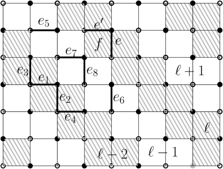
Figure 10.

• if $b^{\prime}$ is at or higher than edge $e_{3}$, then $b^{+}$ is at or higher than $e_{5}$ and $I^{-}_{b^{+}}$ is the same, irrespectively of whether $b$ is at $e$ or $e^{\prime}$. On the other hand, edges $e_{7},e_{8}$ are accessible to $b^{-}$ if $b$ is at $e^{\prime}$ and are not if $b^{-}$ is at $e$, so $|I^{+}_{b^{-}}|$ differs by $2$ in the two cases. Altogether, when $b$ is moved from $e$ to $e^{\prime}$, the contribution of $b^{-}$ to the change of $|\Omega_{\sigma}|-|\Omega_{\sigma}^{(-1)}|$ is $+2$, as desired;

• symmetrically, when $b^{\prime}$ is at or lower than $e_{4}$ then $b^{-}$ is at or lower than $e_{6}$. When $b$ is moved from $e$ to $e^{\prime}$, $I^{+}_{b^{-}}$ does not change, while $|I^{-}_{b^{+}}|$ decreases by $2$, since $e_{7},e_{8}$ are not available positions any more. Again, we get a change $+2$ for $|\Omega_{\sigma}|-|\Omega_{\sigma}^{(-1)}|$, this time coming from $b^{+}$.

• finally, suppose that $b^{\prime}$ is at $e_{1}$ or $e_{2}$. If $b$ is at $e$ then position $e_{7}$ is available for $b^{+}$ and $e_{8}$ is not available for $b^{-}$, while if $b$ is at $e^{\prime}$ the opposite holds. As a consequence, both $b^{+}$ and $b^{-}$ contribute $+1$ to the change of $|\Omega_{\sigma}|-|\Omega_{\sigma}^{(-1)}|$.

∎

Deducing stationarity of $\pi_{\rho}$ on the infinite graph from stationarity of $\pi^{L}_{\rho}$ on the torus works exactly the same on $\mathcal{H}$ or $\mathbb{Z}^{2}$; for definiteness, in Section 8 we will stick to the former case.

5. The discrete Hammersley dynamics (DHD)

On the way towards Theorem 2.4, let us switch for a moment to a one-dimensional interacting particle system known as Discrete Hammersley Dynamics (DHD) [14]. The configuration space of the DHD consists of particle configurations on $\mathbb{Z}$ (at most one particle per site). Each site of $\mathbb{Z}$ has an i.i.d. Poisson clock of rate $1$. When a clock rings at a site $x$, if the site is occupied then nothing happens; otherwise, take the first particle to the right of $x$ and move it to $x$. Note that each particle moves to the left with rate equal to the number $n$ of empty sites before the next particle to the left, and the new position is uniform among the $n$ sites. We call $z_{t}(n)$ the position of the $n^{th}$ particle ($n\in\mathbb{Z}$) at time $t$. Particles are labelled in the initial condition in such a way that $z_{0}(n)<z_{0}(n+1)$, with some arbitrary choice of whom to label $0$ (for instance, it could be the first particle to the right of the origin). Labels do not change as particles move.

The works [1, 28] consider instead the (continuous) Hammersley process [1], which is defined similarly as the DHD, except that particles live on $\mathbb{R}$ instead of $\mathbb{Z}$: again, each particle moves to the left with rate equal to the available space before the next particle and the new position is chosen uniformly in the available interval. In [28] it is proven (among many other results):

Theorem 5.1.

If $\lim_{n\to-\infty}n^{-2}z_{0}(n)=0$, then the dynamics is well defined at all times: the displacement of a particle with respect to the initial position is almost surely finite at all finite times.

Theorem 5.1 extends immediately to the DHD [14] and is obtained with the help of a Harris-type graphical construction, that we recall here. To each site of $\mathbb{Z}$ associate an independent Poisson point process of density $1$ on $\mathbb{R}^{+}$: this is the set of times when the clock at that site rings. Given a realization of all these i.i.d. Poisson processes and given $0\;\leqslant\;s<t$, $-\infty<a<b<\infty$, we can consider the set of all possible up-right paths in the rectangle $(a,b]\times(s,t]$, i.e. sequences $(x_{1},t_{1}),\dots,(x_{n},t_{n})$ of space-time points in the point process in the rectangle, with $x_{1}<\dots<x_{n}$ and $t_{1}<\dots<t_{n}$. Note that inequalities are strict (for times this is not restrictive since with probability one there is at most one clock ringing at a given time). Let as in [1, 28] ${\bf L}((a,s),(b,t))$ be the maximal number of points of the Poisson processes on one such path. Let also

$$\Gamma((a,s),t,k)=\inf\{h\;\geqslant\;0:{\bf L}((a,s),(a+h,t))\;\geqslant\;k\}.$$

Then (this is given in [1, 28] in the continuous Hammersley process where ${\bf L}$ and $\Gamma$ are defined similarly, but the same holds true also for the DHD) for every $t\;\geqslant\;0$

$$z_{t}(n)=\inf_{j\;\leqslant\;n}\{z_{0}(j)+\Gamma((z_{0}(j),0),t,n-j)\}.$$ (5.1)

Note that the DHD has the following monotonicity property:

Lemma 5.2 (Monotonicity for the DHD).

If we take two initial conditions such that $z_{0}(n)\;\leqslant\;z^{\prime}_{0}(n)$ for every $n$ and if we let them evolve using the same Poisson clocks, then the partial order is preserved at all later times.

Proof.

This is immediate from (5.1): if some $z_{0}(j)$ is changed to $z_{0}(j)-a,a\in\mathbb{N}$, then $\Gamma((z_{0}(j),0),t,n-j)$ increases at most by $a$. ∎

The representation (5.1) also allows to get an upper bound on the probability that the displacement of a particle is large. Indeed, if $z_{t}(n)-z_{0}(n)\;\leqslant\;-k$ then there exists $j\;\leqslant\;n$ such that

$${\bf L}((z_{0}(j),0),(z_{0}(j)-k+(z_{0}(n)-z_{0}(j)),t))\;\geqslant\;n-j.$$

With a union bound, the probability (conditionally on the initial positions) that $z_{t}(n)-z_{0}(n)\;\leqslant\;-k$ is upper bounded by

$$\sum_{j<n:z_{0}(j)-z_{0}(n)\;\leqslant\;-k}P({\bf L}((0,0),(0,z_{0}(n)-z_{0}(j)-k,t))\;\geqslant\;n-j),$$ (5.2)

where $P$ denotes the expectation only with respect to the Poisson clocks. One has

$$P({\bf L}((0,0),(h,t))\;\geqslant\;k)\;\leqslant\;(th)^{k}/(k!)^{2}.$$ (5.3)

Indeed, there are $h!/(k!(h-k)!)$ strictly increasing distinct sequences $0<x_{1}<\dots x_{k}\;\leqslant\;h$. Given one of these, the probability that there is an up-right path $(x_{1},t_{1}),\dots,(x_{k},t_{k})$ equals the probability that a Poisson random variable of average $t$ equals at least $k$. On the other hand, if $X$ is a Poisson variable of average $t$ then for $k\;\geqslant\;1$

$$P(X\;\geqslant\;k)=\sum_{n\;\geqslant\;k}e^{-t}\frac{t^{n}}{n!}=\sum_{m\;\geqslant\;0}e^{-t}\frac{t^{m+k}}{(m+k)!}\;\leqslant\;\frac{t^{k}}{k!}.$$ (5.4)

because $(m+k)!\;\geqslant\;k!m!$. Then, (5.3) follows from

$$\frac{h!}{(h-k)!}\frac{1}{k!}\;\leqslant\;\frac{h^{k}}{k!}.$$

Let us call $\mathbb{P}_{z}$ the law of the DHD started from an initial configuration $z=\{z_{0}(n)\}_{n\in\mathbb{Z}}$. From (5.3) we have then

$$\mathbb{P}_{z}(z_{t}(n)-z_{0}(n)\;\leqslant\;-k)\;\leqslant\;\sum_{j<n:z_{0}(j)-z_{0}(n)\;\leqslant\;-k}\frac{t^{n-j}(z_{0}(n)-z_{0}(j)-k)^{n-j}}{((n-j)!)^{2}}.$$ (5.5)

This bound will be used in Section 7.

6. The process started from $\pi_{\rho}$ is well-defined

Here we prove “the first (and easier) half” of Theorem 2.4, i.e. the bead displacement is finite for almost every initial condition sampled from $\pi_{\rho}$.

Proposition 6.1.

Suppose that the initial configuration $\sigma$ is in the set

$$Y=\{\sigma:\text{ for every $\ell$, }\lim_{n\to\infty}n^{-2}z_{0}(\ell,n)=0=\lim_{n\to\infty}n^{-2}z_{0}(\ell,-n)\}.$$ (6.1)

Then the process is well-defined at all times: for every $(\ell,n)$, almost surely $z_{t}(\ell,n)-z_{0}(\ell,n)$ as defined in (2.4) is finite for all $t\;\geqslant\;0$.

Actually, when $q=0$ (resp. when $p=0$) the condition $\lim_{n\to\infty}n^{-2}z_{0}(\ell,-n)=0$ (resp. $\lim_{n\to\infty}n^{-2}z_{0}(\ell,n)=0$) is not necessary. Note also that $\pi_{{\rho}}(Y)=1$ for any non-extremal slope. Indeed, $z_{0}(\ell,n)$ is just the sum of the first $n$ inter-bead distances along column $\ell$. Since the measure $\pi_{{\rho}}$ is ergodic for the action of $\mathbb{Z}^{2}$, $n^{-1}z_{0}(\ell,n)$ converges $\pi_{{\rho}}$-almost surely to the finite limit $1/\rho_{3}$.

Proof of Proposition 6.1.

Fix some column $\ell$. We want to prove that, say, $z_{t}(\ell,n;K)-z_{0}(\ell,n)$ is almost surely bounded away from minus infinity, uniformly in $K$ and for every $n$. Take the DHD slowed down by a factor $q$ (i.e. its clocks ring with rate $q$ and not $1$) with initial condition $z_{0}(n)=z_{0}(\ell,n)$ for every $n$ and couple the DHD and the bead dynamics by establishing that the $q$-clocks (within distance $K_{q}$ from the origin) on column $\ell$ of the lozenge dynamics are the same as the corresponding clocks of the DHD (the DHD has no $p$-clock). Then, bead positions are dominated by those of the DHD, in the sense that $z_{t}(n)\;\leqslant\;z_{t}(\ell,n;K)$ for all times and for all $n$. In fact, call $s_{i},i\;\geqslant\;1$ the ordered times when one of the finitely many clocks in column $\ell$ of the dynamics $X_{t;K}$ ring. We have $z_{0}(\cdot)\;\leqslant\;z_{0}(\ell,\cdot;K)$ (actually with equality). At time $s_{1}^{-}$ the inequality is still true, since the beads in $\ell$ have not moved while some DHD particles may have moved to the left. At time $s_{1}$, one of the following cases occurs:

• a $p$-clock rings. Then, a bead might move upward and nothing happens for the DHD. We have in this case obviously

  $$z_{s_{1}^{+}}(\cdot)\;\leqslant\;z_{s_{1}^{+}}(\ell,\cdot;K).$$ (6.2)

• a $q$-clock rings at an edge $e$ within distance $K_{q}$ from the origin, but no bead can be moved to $e$ without pushing other beads. Again (6.2) holds (for the DHD, a particle can move to the left).

• a $q$-clock rings at an edge $e$ within distance $K_{q}$ from the origin and the bead just above it, call $(\ell,n)$ its label, can be moved to $e$. By assumption, for the DHD, the first particle at position greater or equal to $e$ has index $m\;\geqslant\;n$. After the update, for the DHD one has particle $m$ at $e$ and for the lozenge process one has bead $(\ell,n)$ at $e$. All other particles/beads are unchanged. Clearly then (6.2) holds also in this case.

The argument is then repeated inductively starting from time $s_{1}^{+}$.

Since, by Theorem 5.1, $z_{t}(n)-z_{0}(n)>-\infty$ almost surely, we conclude that $z_{t}(\ell,n;K)-z_{0}(\ell,n)$ is almost surely bounded away from $-\infty$, uniformly in $K$. ∎

7. Large gaps and propagation of information

Let $B_{R}$ be the ball of radius $R$ centered at the origin of $\mathcal{H}$.

Definition 7.1.

Let $\Delta(R,t)$ be the largest integer $n$ such that there exist horizontal edges $e_{1}\in B_{R}$ and $e_{2}$ on the same column of $e_{1}$, at distance $n$ from it, such that at time $t$ there is no bead between them. Also, let $\Delta(R,\;\leqslant\;t)=\sup\{\Delta(R,s),s\;\leqslant\;t\}$.

We need a preliminary result, giving an upper bound on the probability of having a large gap among beads. We start from the case of the torus:

Lemma 7.2.

For $\zeta\in\mathbb{N}$ there exists a constant $C=C_{\zeta}$ such that, for all $T>0,R\;\geqslant\;1$ and $L$ large enough,

$$\int\pi^{L}_{\rho}(d\sigma)\mathbb{P}_{\sigma}[\Delta(R,\;\leqslant\;T)\;\geqslant\;C_{\zeta}\log R]\;\leqslant\;T\frac{C_{\zeta}}{R^{\zeta}}.$$ (7.1)

To be precise, the constant $C_{\zeta}$ also depends on the density vector $\rho$ (through the constant $C(\lambda,u,\rho)$ of Lemma A.1); in this section, for lightness of notation, we often keep the $\rho$ dependence implicit.

Proof of Lemma 7.2.

From Lemma A.1 and convergence of $\pi^{L}_{\rho}$ to $\pi_{\rho}$ it is easy to see that, for $L$ large enough,

$$\pi_{\rho}^{L}(\Delta(R,0)\;\geqslant\;C_{\zeta}\log R)\;\leqslant\;C_{\zeta}R^{-\zeta}$$ (7.2)

if $C_{\zeta}$ is chosen sufficiently large. Using stationarity of $\pi^{L}_{\rho}$, this holds for every fixed $t\;\geqslant\;0$. Then,

$$\mathbb{E}_{\pi^{L}_{\rho}}\left(\int_{0}^{T+1}{\bf 1}_{\{\Delta(R,t)\;\geqslant\;C_{\zeta}\log R\}}dt\right)\;\leqslant\;(T+1)C_{\zeta}\,R^{-\zeta}.$$ (7.3)

Let

$$\tau=\inf\{t>0:\Delta(R,t)>2C_{\zeta}\log R\}$$ (7.4)

and observe that, after time $\tau$, a clock has to ring in the ball $B_{R+C_{\zeta}\log R}$ before $\Delta(R,t)$ becomes strictly smaller than $C_{\zeta}\log R$ (this is just a necessary condition: not every ring in $B_{R+C_{\zeta}\log R}$ decreases $\Delta(R,t)$). Note that the realization of the Poisson clock rings at times $t>\tau$ is independent of the process up to $\tau$ (and of $\tau$ itself). On the other hand, with probability $u$ uniformly bounded away from zero, none of the $O(R^{2})$ clocks in $B_{R+C_{\zeta}\log R}$ rings in the time lag $[\tau,\tau+1/R^{2}]$. In conclusion,

$$\mathbb{E}_{\pi^{L}_{\rho}}\left(\left.\int_{0}^{T+1}{\bf 1}_{\{\Delta(R,t)\;\geqslant\;C_{\zeta}\log R\}}dt\right|\tau\;\leqslant\;T\right)\;\geqslant\;u/R^{2}.$$ (7.5)

Together with (7.3) we get that

$$\mathbb{P}_{\pi^{L}_{\rho}}(\tau\;\leqslant\;T)\;\leqslant\;(T+1)C_{\zeta}R^{2-\zeta}/u.$$ (7.6)

We conclude by observing that $\{\tau\;\leqslant\;T\}=\{\Delta(R,\;\leqslant\;T)>2C_{\zeta}\log R\}$ and recalling that $\zeta$ can be chosen as large as wished. ∎

For the dynamics on $\mathcal{H}$ the same argument does not work since we do not know (yet) that $\pi_{\rho}$ is stationary. A similar result however still holds, but the proof requires a comparison with the DHD we introduced above:

Lemma 7.3.

For any $T<\infty,\zeta\in\mathbb{N}$ there exists a constant $C=C(\zeta,T)$ such that for $R$ large

$$\int\pi_{\rho}(d\sigma)\mathbb{P}_{\sigma}[\Delta(R,\;\leqslant\;T)\;\geqslant\;C\log R]\;\leqslant\;\frac{C}{R^{\zeta}}.$$ (7.7)

A useful variant of Lemma 7.3 that we will use later (and whose proof follows almost exactly the same argument) is:

Corollary 7.4.

Fix a horizontal edge $e$ and a time $T>0$. For $n^{\pm}\;\geqslant\;0$ let $A_{T,n^{+},n^{-}}$ be the event that there exists a time $s\;\leqslant\;T$ and horizontal edges $e^{\pm}$ on the same column as $e$, with $e^{+}$ at distance $n^{+}$ above $e$ and $e^{-}$ at distance $n^{-}$ below it, such that at time $s$ there is a bead at $e^{\pm}$ and no bead between them. There exists $C=C(\rho,T)$ such that

$$\mathbb{P}_{\pi_{\rho}}(A_{T,n^{+},n^{-}})\;\leqslant\;Ce^{-(1/C)(n^{+}+n^{-})}.$$ (7.8)

For the proof of Lemma 7.3 we need the following preliminary result:

Lemma 7.5.

Recall that $\hat{\pi}_{\rho}$ is the Gibbs measure conditioned to have a bead at $e_{0}$ and that $\phi_{t}-\phi_{0}$ is the displacement of the tagged bead at time $t$. Then, for every $T>0$ there exists a positive constant $a=a(\rho,T)$ such that for every $D\;\geqslant\;0$

$$\mathbb{P}_{\hat{\pi}_{\rho}}(\exists t\;\leqslant\;T:|\phi_{t}-\phi_{0}|\;\geqslant\;D)\;\leqslant\;a\exp(-D/a).$$ (7.9)

Proof of Lemma 7.5.

To fix ideas let us prove that

$$\mathbb{P}_{\hat{\pi}_{\rho}}(\exists t\;\leqslant\;T:\phi_{t}-\phi_{0}\;\leqslant\;-D)\;\leqslant\;a\exp(-D/a).$$ (7.10)

We have seen in the proof of Proposition 6.1 that the downward displacement of a bead $b$ is at all times stochastically smaller than the leftward displacement of a DHD particle (for the DHD with clocks of rate $q$) up to the same time, started from a configuration where the particles are at the same position as the beads in the column corresponding to $b$. Since the DHD particles move only to the left, the event $\{\exists t\;\leqslant\;T:\phi_{t}-\phi_{0}\;\leqslant\;-D\}$ means that the DHD particle corresponding to $b$ has moved more than $D$ by the non-random time $T$.

Call $n$ the label of the tagged bead $b$ in its column, initially at position $z_{0}(n):=e_{0}$, and go back to (5.5). Observe that if $z_{0}(n)-z_{0}(n-r)\;\geqslant\;u$ then there are at most $r$ beads in a set of $u$ adjacent horizontal edges below $z_{0}(n)$. Using Lemma A.1 we see that, except with probability exponentially small in $D$, one has

$$z_{0}(n)-z_{0}(n-r)<\frac{1}{\varepsilon(\rho)}\max\left[r,\varepsilon(\rho)D\right]\quad\text{ for every }r\;\geqslant\;1$$ (7.11)

for some positive $\varepsilon$ depending only on the slope $\rho$. Then, from (5.5), on the event (7.11)

$$\mathbb{P}_{z}(z_{T}(n)-z_{0}(n)\;\leqslant\;-D)\;\leqslant\;\sum_{r>\varepsilon(\rho)D}\frac{T^{r}(r/\varepsilon(\rho))^{r}}{(r!)^{2}}\;\leqslant\;c(\rho,T)\,e^{-c^{\prime}(\rho,T)D\log D}$$ (7.12)

that decays super-exponentially in $D$. ∎

Proof of Lemma 7.3.

On the event $\Delta(R,\;\leqslant\;T)\;\geqslant\;C\log R$ there exists a time $s\;\leqslant\;T$ and a horizontal edge $e\in B_{R}$ such that at time $s$ there is no bead in the $C\log R$ horizontal edges immediately above or immediately below $e$. Assume w.l.o.g. that the former is the case. Let $e^{+}$ (resp. $e^{-}$) be the lowest horizontal edge above $e$ (resp. the highest edge below $e$) where there is some bead $b^{+}$ (resp. $b^{-}$) at time $s$. Call $N\;\geqslant\;C\log R$ the distance between $e^{+}$ and $e^{-}$. There are two possible cases:

• at time zero bead $b^{+}$ is within distance $N/10$ from $e^{+}$ and similarly $b^{-}$ is within distance $N/10$ from $e^{-}$. This implies that at time zero there is no bead in a vertical interval of length $N/2$, centered on the face at distance $N/2$ above $e$. Since in the stationary measure the distance between neighboring beads has exponential tails (Lemma A.1) and $N\;\geqslant\;C\log R$, this event has probability

  $$O\left(R^{2}\exp\left(-a(\rho)\,C\log R\right)\right)$$

  for some positive $a$ depending only on the slope $\rho$, where the factor $R^{2}$ comes from a union bound over all possible positions of $e$. Choosing $C=C_{\zeta}$ sufficiently large, we get a $O(R^{-\zeta})$ bound.

• At time zero, either $b^{+}$ is at distance $n\;\geqslant\;N/10$ from $e^{+}$, or $b^{-}$ is at distance $m\;\geqslant\;N/10$ from $e^{-}$. Say, to fix ideas, that the former is the case. This implies that at the (random) time $s\;\leqslant\;T$ the bead $b^{+}$ has moved, say downward, a distance $n\;\geqslant\;N/10$ with respect to the initial position. Thanks to Proposition 7.5, this has probability exponentially small in $n$. Summing over $n\;\geqslant\;N/10$, over the possible values of $N\;\geqslant\;C\log R$ and over the the $O(R^{2})$ possible positions of $e$ gives a bound $O(R^{-\zeta})$ if $C$ is chosen large enough.

∎

As an application, we show that information does not propagate instantaneously through the system: if two initial conditions sampled from equilibrium differ only outside a ball of radius $R$, it is very unlikely that in a short time the discrepancy propagates to reach the center of the ball. It is useful to give a proof of this fact, since an extremely similar argument will provide the proof of Theorem 2.4. For usual short-range systems one has a ballistic propagation bound: information does not travel more than a distance $const\times t$ in a time interval $t$ (cf. for instance [25, Sec. 3.3]). The situation is more intricate here due to the presence of a-priori unbounded gaps among beads.

Let the pair $(\sigma,\sigma^{\prime})\in\Omega_{\mathcal{H}}^{\otimes 2}$ be distributed according to some law $\nu$ such that $\sigma\sim\pi_{\rho}$, $\sigma^{\prime}\sim\pi_{\rho}$ and $\sigma,\sigma^{\prime}$ coincide in $B_{R}$. Couple the two processes by using the same Poisson clocks for both and call $\mathbb{P}_{\nu}$ the law of the joint process $(\sigma_{t},\sigma^{\prime}_{t})$. Let $\delta_{e}(t)\in\{0,1\}$ (resp. $\delta^{\prime}_{e}(t)\in\{0,1\}$) be the bead occupation variable at time $t$ at a fixed horizontal edge $e$ (say at the center of $B_{R}$) for the process started from $\sigma$ (resp. $\sigma^{\prime}$). Let also $\Delta_{max}=\max(\Delta(R,\;\leqslant\;T),\Delta^{\prime}(R,\;\leqslant\;T))$, with $\Delta^{\prime}(R,\;\leqslant\;T)$ referring to the process started from $\sigma^{\prime}$.

Proposition 7.6.

For every $T<\infty,\zeta\in\mathbb{N}$ there is a constant $C$ such that

$$\mathbb{P}_{\nu}((\delta_{e}(t))_{t\in[0,T]}\not\equiv(\delta^{\prime}_{e}(t))_{t\in[0,T]})\;\leqslant\;\frac{C}{R^{\zeta}}.$$ (7.13)

Proof of Proposition 7.6.

We have from Lemma 7.3

$$\mathbb{P}_{\nu}((\delta_{e}(t))_{t\in[0,T]}\not\equiv(\delta^{\prime}_{e}(t))_{t\in[0,T]})$$ (7.14)

$$\;\leqslant\;\mathbb{P}_{\nu}\left[(\delta_{e}(t))_{t\in[0,T]}\not\equiv(\delta^{\prime}_{e}(t))_{t\in[0,T]};\Delta_{max}\;\leqslant\;C_{\zeta}\log R\right]+C_{\zeta}/R^{\zeta}.$$ (7.15)

On the event $(\delta_{e}(t))_{t\in[0,T]}\not\equiv(\delta^{\prime}_{e}(t))_{t\in[0,T]}$ call $t_{1}\;\leqslant\;T$ the first time when $\delta_{e}(t_{1})\neq\delta^{\prime}_{e}(t_{1})$. There are two possible cases:

1. $\delta_{e}(t_{1}^{-})=\delta^{\prime}_{e}(t_{1}^{-})=1$ and say $\delta_{e}(t_{1})=0\neq\delta^{\prime}_{e}(t_{1})=1$. In this case at $t_{1}$ a clock rings in the column $0$ (the one of $e$) at a horizontal edge $x_{1}$ within distance $\Delta_{max}$ from $e$ and in configuration $\sigma^{\prime}_{t_{1}^{-}}$ (but not in $\sigma_{t_{1}^{-}}$) a bead in a neighboring column is preventing the bead at $e$ to move to $x_{1}$. At time $t_{1}$ there is therefore a horizontal edge $e_{1}$ in column $\pm 1$, with distance within $\Delta_{max}+1$ from $x_{1}$ (the $+1$ is because it is on the neighboring column), where the bead occupation variable is different.

2. $\delta_{e}(t_{1}^{-})=\delta^{\prime}_{e}(t_{1}^{-})=0$ and say $\delta_{e}(t_{1})=0\neq\delta^{\prime}_{e}(t_{1})=1$. This means that at $t_{1}$ the clock at $e$ rings (in this case we set $x_{1}:=e$) and that in configuration $\sigma_{t_{1}^{-}}$ (but not in $\sigma^{\prime}_{t_{1}^{-}}$) a particle in one of the two neighboring columns is preventing a certain bead (below $e$ if the clock is a $p$-clock and above the origin $e$ if it is a $q$-clock) to reach $e$. In particular, as in case (i), at time $t_{1}$ there is an edge $e_{1}$ in column $\pm 1$ within distance $\Delta_{max}+1$ from $x_{1}$, where the bead occupation variable is different.

Call $t_{2}<t_{1}$ the first time $s$ at which $\delta_{e_{1}}(s)\neq\delta^{\prime}_{e_{1}}(s)$. On the event $\Delta_{max}\;\leqslant\;C_{\zeta}\log R$, we have that $t_{2}>0$ because $e_{1}$ is in the ball $B_{R}$ where initial conditions coincide.

We iterate the argument (cf. Fig. 11), and as before we deduce that at $t_{2}$ there is an edge $x_{2}$ in the column of $e_{1}$, within distance $\Delta_{max}$ from it, where a clock rings and an edge $e_{2}$ in a column neighboring the one of $e_{1}$, and at distance within $\Delta_{max}+1$ from $x_{2}$, where the bead occupation variable is different. The iteration stops when $e_{n}$ is outside the ball $B_{R}$ of radius $R$. Note that $x_{i},x_{i+1}$ are within vertical distance $2(\Delta_{max}+1)\;\leqslant\;3\Delta_{max}$ and horizontal distance $1$ from each other.

Figure 11. An example of the iteration. We have that $|x_{i}-e_{i-1}|\;\leqslant\;\Delta_{max}$ and $|e_{i}-x_{i-1}|\;\leqslant\;(\Delta_{max}+1)$. When $x_{i+1}=e_{i}$ it means that we are in case (ii) above. The arrow follows the chain $x_{1},x_{2},\dots$

Altogether, if $(\delta_{e}(t))_{t\in[0,T]}\not\equiv(\delta^{\prime}_{e}(t))_{t\in[0,T]}$ then either $\Delta_{max}\;\geqslant\;C_{\zeta}\log R$, or there exists:

• a chain of sites $x_{1},\dots,x_{n}$, with $x_{i},x_{i+1}$ on neighboring columns, $x_{1}$ on the column $\ell=0$ and within distance $C_{\zeta}\log R$ from $e$ (the center of the ball $B_{R}$), $|x_{i}-x_{i+1}|\;\leqslant\;3C_{\zeta}\log R$ and $|x_{n}|\;\geqslant\;R/2$;

• a sequence of times $0\;\leqslant\;t_{n}<t_{n-1}<\dots t_{1}\;\leqslant\;T$ such that either the $p$-clock or the $q$-clock at $x_{i}$ rings at time $t_{i}$.

We get with a union bound

$$\mathbb{P}_{\nu}((\delta_{e}(t))_{t\in[0,T]}\not\equiv(\delta^{\prime}_{e}(t))_{t\in[0,T]})\;\leqslant\;C_{\zeta}/R^{\zeta}+\sum_{n\;\geqslant\;R/(6C_{\zeta}\log R)}N_{n}\,P_{n},$$ (7.16)

where $P_{n}$ is the probability that a Poisson variable of average $T(p+q)$ is at least $n$, while $N_{n}$ is the number of all possible distinct chains $x_{1},\dots,x_{n}$ of $n$ sites with the above specified properties. Of course $N_{n}\;\leqslant\;(C^{\prime}_{\zeta}\log R)^{n}$ for some constant $C^{\prime}_{\zeta}$ while (5.4) gives

$$P_{n}\;\leqslant\;e^{-n\log(n/T(p+q))+n}.$$

The sum in (7.16) is $o(R^{-\zeta})$. ∎

Remark 7.7.

Take $\sigma$ sampled from $\pi_{\rho}$ and let $\sigma_{t},\sigma^{\prime}_{t}$ be the coupled processes with the same Poisson clocks and the same initial condition, except that $\sigma_{t}$ has cutoff parameter $K=(K_{p},K_{q})$ and $\sigma^{\prime}_{t}$ has a different cutoff parameter $K^{\prime}=(K^{\prime}_{p},K^{\prime}_{q})$. With the same ideas as for Proposition 7.6 it is possible to prove that

$$\int\pi_{\rho}(d\sigma)\mathbb{P}_{\sigma}((\delta_{e}(t))_{t\in[0,T]}\not\equiv(\delta^{\prime}_{e}(t))_{t\in[0,T]})=\varepsilon(K,K^{\prime})$$ (7.17)

with $\varepsilon(K,K^{\prime})\to 0$ when $\min(K_{p},K^{\prime}_{p},K_{q},K^{\prime}_{q})\to\infty$. From this one can deduce that the order how the cutoffs in (2.4) are removed is irrelevant.

8. Stationarity of Gibbs measures in the infinite graph

We will prove Theorems 2.4 and 2.6 only for the honeycomb lattice. As for square lattice, once the result is proven on the torus (cf. Section 4.2), the extension to the infinite system works exactly the same.

8.1. Proof of Theorem 2.4

Let us first of all prove (2.5) in the case where $f=\prod_{i=1}^{k}\delta_{e_{i}}$, where $e_{1},\dots,e_{k}$ are horizontal edges ($k\in\mathbb{N}$) and $\delta_{e}$ is the indicator function that there is a dimer at $e$. Choose $R$ large enough so that all $e_{i}$ are in the ball $B_{R}$ and say close to its center. Call $\nu_{R}$ (resp. $\nu^{L}_{R}$) the marginal of $\pi_{\rho}$ (resp. $\pi^{L}_{\rho}$) on $B_{R}$ (or, to be pedantic, on $\mathcal{H}\cap B_{R}$) and let $\sigma_{B_{R}}$ be sampled from $\nu_{R}$ and $\sigma^{\prime}_{B_{R}}$ from $\nu^{L}_{R}$. From convergence of $\pi^{L}_{\rho}$ to $\pi_{\rho}$ as $L\to\infty$, we can choose $L$ sufficiently large and a coupling of $(\nu_{R},\nu^{L}_{R})$ such that $\sigma_{B_{R}}=\sigma^{\prime}_{B_{R}}$ except with probability $\varepsilon_{R}$ that tends to zero as $R\to\infty$.

Let $\sigma\in\Omega_{\mathcal{H}}$ and $\sigma^{\prime}\in\Omega_{\mathbb{T}_{L}}$ (with $\Omega_{\mathbb{T}_{L}}$ the set of dimer coverings of $\mathbb{T}_{L}$) be sampled as follows. The restrictions $(\sigma_{B_{R}},\sigma^{\prime}_{B_{R}})$ to $B_{R}$ are sampled from $(\nu_{R},\nu^{L}_{R})$. Given the realization of $(\sigma_{B_{R}},\sigma^{\prime}_{B_{R}})$, the configuration $(\sigma_{\mathcal{H}\setminus B_{R}},\sigma^{\prime}_{\mathbb{T}_{L}\setminus B_{R}})$ outside $B_{R}$ are sampled independently: $\sigma_{\mathcal{H}\setminus B_{R}}$ from $\pi_{\rho}(\cdot|\sigma_{B_{R}})$ and $\sigma^{\prime}_{\mathbb{T}_{L}\setminus B_{R}}$ from $\pi^{L}_{\rho}(\cdot|\sigma^{\prime}_{B_{R}})$. We have therefore that $\sigma\sim\pi_{\rho},\sigma^{\prime}\sim\pi^{L}_{\rho}$ and they coincide in $B_{R}$, except with probability $\varepsilon_{R}$.

Now couple the processes $(\sigma_{t})_{t\;\geqslant\;0},(\sigma^{\prime}_{t})_{t\;\geqslant\;0}$ started from $\sigma,\sigma^{\prime}$ by establishing that the Poisson clocks in $B_{R}$ are the same for the two, while those outside $B_{R}$ are independent. Proceeding exactly like in the proof of Proposition 7.6 and using both Lemma 7.2 and 7.3 to estimate the probability that $\Delta(R,T)\;\geqslant\;C_{\zeta}\log R$ in any of the two processes, one finds that, except with probability $\varepsilon_{R}+R^{-\zeta}=\varepsilon^{\prime}_{R}$, the bead occupation variables at all edges $e_{i},i\;\leqslant\;k$ for the two processes coincide up to time $T$. Therefore, for every $t\;\leqslant\;T$,

$$\mathbb{E}_{\pi_{\rho}}(f(X_{t}))=\mathbb{E}_{\pi^{L}_{\rho}}(f(X_{t}))+\varepsilon^{\prime}_{R}=\pi^{L}_{\rho}(f)+\varepsilon^{\prime}_{R}=\pi_{\rho}(f)+\varepsilon^{\prime}_{R}+\varepsilon^{\prime\prime}_{L}$$ (8.1)

where we used Proposition 4.1 (stationarity on the torus) in the second equality. Arbitrariness of $T<\infty$ and of $R$ proves (2.5) in the particular case $f=\prod_{i=1}^{k}\delta_{e_{i}}$ (the larger $T$ is, the larger we have to choose $R$ and therefore $L$).

When $f$ is any bounded local function depending only on the configuration of the horizontal dimers, it is always possible to write $f$ as a finite linear combination of functions of the form $\prod_{i=1}^{k}\delta_{e_{i}}$, so the claim of the theorem holds also in this case.

Finally, it remains to consider the case where $f$ is a local function depending also on the configuration of non-horizontal edges. This requires a slightly different argument.

Let us start with a simple observation, see Fig. 12.

Figure 12. Given the horizontal dimers at $a,b,c,d$, all the dimer occupation variables at edges of hexagons $s_{1},\dots,s_{k}$ is determined. In fact, all north-east oriented edges between $a$ and $c$ and between $d$ and $b$ are occupied by dimers, and the same is for south-east edges between $c$ and $b$ or between $a$ and $d$.

Let $a,b$ be two horizontal edges in the same column $\ell$ and let $s_{1},\dots,s_{k}$ be the hexagons of $\ell$ included between $a,b$. If we know that the only beads in $s_{1},\dots s_{k}$ are at $a,b$ and if we also know the location of the two beads, one in column $\ell+1$ and one in column $\ell-1$, whose vertical coordinate is between that of $a$ and of $b$, then we can reconstruct unambiguously the dimer occupation variables of all edges (not just horizontal ones) of hexagons $s_{1},\dots,s_{k}$.

Call $S$ a finite collection of hexagons such that the union of their edges contains the support of $f$. Let $\Lambda_{K}$ be the collection of hexagons that are at graph distance (on $\mathcal{H}^{*}$) at most $K$ from $S$ ($S$ itself is a subset of $\Lambda_{K}$). Let $E_{K}$ be the event that, for every $s\in S$, there are two beads in $\Lambda_{K}$, one below $s$ and one above it. From the discussion above we know that, on the event $E_{K}$, the dimer configuration on all the hexagons in $S$ is uniquely identified by $\eta|_{\Lambda_{K}}$, the bead configuration in $K$. Let

$$g(\eta):=g(\eta|_{\Lambda_{K}})=f(\sigma)1_{E_{\Lambda_{K}}}$$ (8.2)

which depends only on $\eta|_{\Lambda_{K}}$. Let also $\tilde{E}_{K}(t)$ the event that $E_{K}$ is realized at every $s\;\leqslant\;t$. We have

$$\mathbb{E}_{\pi_{{\rho}}}(f(X_{t}))=\mathbb{E}_{\pi_{{\rho}}}(g(\eta_{t});1_{\tilde{E}_{K}(t)})+O(\|f\|_{\infty}\mathbb{P}_{\pi_{\rho}}(\tilde{E}_{K}(t)^{c}))$$ (8.3)

$$=\mathbb{E}_{\pi_{{\rho}}}(g(\eta_{t}))+O(\|f\|_{\infty}\mathbb{P}_{\pi_{\rho}}(\tilde{E}_{K}(t)^{c})).$$ (8.4)

From Corollary 7.4 we deduce easily that $\varepsilon_{K,t}:=\mathbb{P}_{\pi_{\rho}}(\tilde{E}_{K}(t)^{c})$ tends to zero as $K\to\infty$, for every fixed $t$. Therefore,

$$\mathbb{E}_{\pi_{{\rho}}}(f(X_{t}))=\mathbb{E}_{{\pi_{\rho}}}(g(\eta_{t}))+O(\|f\|_{\infty}\varepsilon_{K,t})$$ (8.5)

$$={\pi_{\rho}}(g)+O(\|f\|_{\infty}\varepsilon_{K,t})=\pi_{\rho}(f)+O(\|f\|_{\infty}\varepsilon_{K,t})$$ (8.6)

where we used invariance of the Gibbs measure for functions of the bead configuration in the second equality and

$$\pi_{{\rho}}(g)=\pi_{{\rho}}(f)+O(\|f\|_{\infty}\varepsilon_{K,0})$$

in the last (note $\varepsilon_{K,0}\;\leqslant\;\varepsilon_{K,t}$). We conclude by letting $K\to\infty$.

8.2. Proof of Proposition 2.6

This is very similar to the proof of Theorem 2.4, so we will be very sketchy. Given any $R>0$ and $\varepsilon>0$ one can choose $L$ sufficiently large so that there is a probability law for the random couple $(\sigma,\sigma^{\prime})\in\Omega_{\mathcal{H}}\times\Omega_{\mathbb{T}_{L}}$ such that $\sigma\sim\hat{\pi}_{\rho},\sigma^{\prime}\sim\hat{\pi}^{L}_{\rho}$ and $\sigma,\sigma^{\prime}$ coincide, except with probability $\varepsilon$, in the ball $B_{R}$. This is done like at the beginning of the proof of Theorem 2.4: in fact, the total variation distance between the marginals on $B_{R}$ of $\hat{\pi}_{\rho},\hat{\pi}^{L}_{\rho}$ tends to zero as $L\to\infty$ (this is because the statement is true for the measures $\pi_{\rho},\pi^{L}_{\rho}$ not conditioned to have a bead at the edge $e_{0}$, and the probability to have a bead at $e_{0}$ is uniformly bounded away from zero). As in Theorem 2.4, given any $a>0$, the coupled bead processes $(\sigma_{t},\sigma^{\prime}_{t})$ that use the same clocks in $B_{R}$ coincide up to time $T$ in the ball $B_{a}$, except with probability $\varepsilon$, provided $R$ is larger than some $R_{0}(a,T)$. On the other hand, by comparing the displacement of a bead with that of a DHD particle, we see that if $a$ is sufficiently large (depending only on $T$) the “tagged bead” stays within distance $a/2$ from its initial position up to time $T$, except with probability $\varepsilon$. In conclusion, the processes $\hat{X}_{t},\hat{X}_{t}^{\prime}$ re-centered at the position of the tagged bead of $\sigma_{t},\sigma^{\prime}_{t}$ coincide (except with probability $2\varepsilon$) up to time $T$ in a ball of radius $a/2$ centered at the origin. Together with the fact that the re-centered process $\hat{X}_{t}^{\prime}$ has law $\hat{\pi}^{L}_{\rho}$ at all times (Proposition 4.2) this implies the claim.

9. Speed and fluctuations

Here we prove Theorem 3.1 and 3.2 about average speed and fluctuations of the growth process.

Let $\Lambda$ be the $\ell\times\ell$ box in $\mathcal{H}$ defined as the collection of hexagons obtained by translating a fixed hexagonal face $x$ (say, the one at the origin of $\mathcal{H}$) by $a\vec{e}_{1}+b\vec{e}_{2},0\;\leqslant\;a,b\;\leqslant\;\ell$. Let

$$Q_{\Lambda}(t)=\sum_{x\in\Lambda}(h_{x}(t)-h_{x}(0))=\sum_{x\in\Lambda}Q_{x}(t).$$ (9.1)

Remark that

$$Q_{\Lambda}(t+\delta)=Q_{\Lambda}(t)-\sum_{e}y^{(p)}_{e}|V(e,\uparrow)\cap\Lambda|+\sum_{e}y^{(q)}_{e}|V(e,\downarrow)\cap\Lambda|+R_{\Lambda,t,\delta}$$ (9.2)

with $y^{(p)}_{e}/y^{(q)}_{e}$ the indicator that the $p/q$-clock at $e$ rings once in the time interval $[t,t+\delta]$, while the “error term” $R_{\Lambda,t,\delta}$ includes the contribution to the change of $Q_{\Lambda}$ from the events where there are $n\;\geqslant\;2$ edges $e_{1},\dots,e_{n}$ where clocks ring in the time interval $[t,t+\delta]$ and where, for every $i\;\leqslant\;n$, either $|V(e_{i},\downarrow)\cap\Lambda|\neq 0$ or $|V(e_{i},\uparrow)\cap\Lambda|\neq 0$.

Proof of (3.1).

We want to see that

$$\mathbb{E}_{\pi_{\rho}}[Q_{\Lambda}(t)]=(q-p)t\ell^{2}J$$ (9.3)

with $J$ defined in (3.2). By linearity we can assume $\ell=1$, i.e. $\Lambda=\{x\}$.

To see that $R_{\{x\},t,\delta}$ can be neglected for $\delta\to 0$ let $b^{\pm}(t)$ be the lowest/highest bead above/below $x$ in the same column and let $I(t)$ be the collection of horizontal edges included between $b^{-}(t)$ and $b^{+}(t)$. Let also $I(t,\delta)=\cup_{s\in[t,t+\delta]}I(s)$. Then, observe that the only clock rings that can contribute $\pm 1$ to $Q_{x}(t+\delta)-Q_{x}(t)$ necessarily occur in $I(t,\delta)$. Then,

$$|R_{\{x\},t,\delta}|\;\leqslant\;N\,1_{\{N\;\geqslant\;2\}}$$ (9.4)

where $N$ is a Poisson variable of average $\delta(p+q)|I(t,\delta)|$. Note that the law of $|I(t,\delta)|$ for the stationary process of law $\mathbb{P}_{\pi_{\rho}}$ is independent of $t$ and that, from Corollary 7.4, the random variable $|I(0,\delta)|$ has exponential tails. Therefore, $\mathbb{E}_{\pi_{\rho}}|R_{\{x\},t,\delta}|=O(\delta^{2})$ and we see that

$$\frac{d}{dt}\mathbb{E}_{\pi_{\rho}}[Q_{x}(t)]=-p\,\pi_{\rho}(|\{e:x\in V(e,\uparrow)\}|)+\,q\,\pi_{\rho}(|\{e:x\in V(e,\downarrow)\}|)$$ (9.5)

$$=(q-p)\pi_{\rho}(|\{e:x\in V(e,\uparrow)\}|)$$ (9.6)

where we used stationarity of $\pi_{\rho}$ and in the last step its invariance by reflections through any hexagon. ∎

Proof of (3.3) and (3.8).

We compute the variance of $Q_{\Lambda}(t)$. We have (recall (9.2), where again we can see that $R_{\Lambda,t,\delta}\approx\delta^{2}$ for $\delta$ small with the same argument as above), letting for lightness of notation $\langle\cdot\rangle:=\mathbb{E}_{\pi_{\rho}}$,

$$\frac{d}{dt}\mathbb{\langle}Q_{\Lambda}(t)^{2}\rangle=2\langle Q_{\Lambda}(t)K_{1}(\sigma_{t})\rangle+\langle K_{2}(\sigma_{t})\rangle$$ (9.7)

where

$$K_{n}(\sigma)=(-1)^{n}p\sum_{e}|V(e,\uparrow)\cap\Lambda|^{n}+q\sum_{e}|V(e,\downarrow)\cap\Lambda|^{n}$$ (9.8)

and the sums run over all horizontal edges of $\mathcal{H}$. We have then, recalling also (9.3), $\langle K_{2}(\sigma_{t})\rangle=\pi_{\rho}(K_{2})$ and $\partial_{t}\langle Q_{\Lambda}(t)\rangle=\pi_{\rho}(K_{1})$,

$$\frac{d}{dt}M_{2}(t):=\frac{d}{dt}\langle(Q_{\Lambda}(t)-\langle Q_{\Lambda}(t)\rangle)^{2}\rangle=2\langle(Q_{\Lambda}(t)-\langle Q_{\Lambda}(t)\rangle)(K_{1}(\sigma_{t})-\pi_{\rho}(K_{1}))\rangle$$ (9.9)

$$+\pi_{\rho}(K_{2}).$$ (9.10)

One has (see Appendix A) that

$$\sup_{\ell}\ell^{-2}\pi_{\rho}(|K_{n}|)\;\leqslant\;C_{1}=C_{1}(n)<\infty$$ (9.11)

and, for every $\delta>0$,

$$\sup_{\ell}\frac{1}{\ell^{2+\delta}}\pi_{\rho}[(K_{1}-\pi_{\rho}(K_{1}))^{2}]\;\leqslant\;C_{2}(\delta)<\infty.$$ (9.12)

Remark 9.1.

It is likely that the variance of $K_{1}$ is actually of order $\ell^{2}$, without any spurious correction. Indeed it is proven in [7] that, if $f$ is a local dimer function and $f_{x}$ is $f$ translated by $x\in\mathbb{Z}^{2}$, then $(1/\ell)\sum_{|x|\;\leqslant\;\ell}[f_{x}-\pi_{\rho}(f_{x})]$ satisfies a CLT with finite variance. The problem with $K_{1}$ is that $|V(e,\uparrow)\cap\Lambda|,|V(e,\downarrow)\cap\Lambda|$ are not local functions. While in principle they are “almost-local” (the probability that they involve more than $n$ dimers decays at least exponentially in $n$, see Lemma A.1), even proving the weaker (9.12) requires some non-trivial work.

We have from (9.9), from stationarity and from (9.11), (9.12)

$$\frac{d}{dt}M_{2}(t)\;\leqslant\;\sqrt{M_{2}(t)}\sqrt{\pi_{\rho}[(K_{1}(\sigma_{t})-\pi_{\rho}(K_{1}))^{2}]}+2\ell^{2}C_{1}$$ (9.13)

$$\;\leqslant\;C_{3}(\delta)\ell^{1+\delta/2}\sqrt{M_{2}(t)}+2\ell^{2}C_{1}$$ (9.14)

from which it is then immediate to deduce that

$$M_{2}(t=\ell)\;\leqslant\;C_{4}\ell^{4+\delta}.$$ (9.15)

Now we are ready to prove (3.3). Let $x_{0}$ be a face in $\Lambda$. Write

$$\mathbb{P}_{\pi_{\rho}}(|Q_{x_{0}}(\ell)-\langle Q_{x_{0}}(\ell)\rangle|\;\geqslant\;\ell^{2\delta})$$ (9.16)

$$\;\leqslant\;\mathbb{P}_{\pi_{\rho}}(|Q_{x_{0}}(\ell)-\langle Q_{x_{0}}(\ell)\rangle|\;\geqslant\;\ell^{2\delta};|Q_{\Lambda}(\ell)-\langle Q_{\Lambda}(\ell)\rangle|\;\leqslant\;\ell^{2+\delta})+o(1)$$ (9.17)

where we used (9.15) to neglect the event that $|Q_{\Lambda}(\ell)-\langle Q_{\Lambda}(\ell)\rangle|\;\geqslant\;\ell^{2+\delta}$. On the other hand

$$Q_{\Lambda}(\ell)-\langle Q_{\Lambda}(\ell)\rangle=-A_{1}+A_{2}+A_{3}$$ (9.18)

$$:=-\sum_{x\in\Lambda}[h_{x}(0)-h_{x_{0}}(0)-\pi_{\rho}(h_{x}-h_{x_{0}})]$$ (9.19)

$$+\sum_{x\in\Lambda}[h_{x}(\ell)-h_{x_{0}}(\ell)-\pi_{\rho}(h_{x}-h_{x_{0}})]+\ell^{2}[Q_{x_{0}}(\ell)-\langle Q_{x_{0}}(\ell)\rangle].$$ (9.20)

We have (see again Appendix A)

$$\pi_{\rho}\left[A_{1}^{2}\right]=O(\ell^{4}\log\ell)$$ (9.21)

so that, using stationarity and Tchebyshev,

$$|A_{1}|,|A_{2}|\;\leqslant\;\ell^{2}\log\ell,$$ (9.22)

with probability $1-o(1)$. Finally, we note that if event (9.22) holds and at the same time $|Q_{\Lambda}(\ell)-\langle Q_{\Lambda}(\ell)\rangle|\;\leqslant\;\ell^{2+\delta}$, one cannot have $|Q_{x_{0}}(\ell)-\langle Q_{x_{0}}(\ell)\rangle|\;\geqslant\;\ell^{2\delta}$. Eq. (3.3) is then proven (just let $\ell:=t$).

Remark 9.2.

If for a given slope $\rho$ the condition (3.7) is satisfied, then one can prove (cf. Remark A.2 below) that $\pi_{\rho}[(K_{1}-\pi_{\rho}(K_{1}))^{2}]=O(\ell^{2}\log\ell)$, to be compared with (9.12). Going back to (9.13) one sees that (9.15) is then improved to $M_{2}(t=\ell)\;\leqslant\;C_{4}\ell^{4}\log\ell$. Repeating the argument that starts with (9.16), one sees immediately that (3.3) is improved into (3.8).

∎

Appendix A Some equilibrium estimates

Here we give upper bounds on the probability that, at equilibrium, there is a large gap between two consecutive beads in the same column. We use this information to deduce several useful equilibrium estimates.

Let $J_{r}$ be a set of $r$ adjacent horizontal edges in the same vertical column of $\mathcal{H}$ and $N_{r}$ the number of beads in $J_{r}$.

Lemma A.1.

Let $\rho$ be a non-extremal slope. For every $\lambda>0$ and $u>0$ there exists $C=C(\lambda,u,\rho)<\infty$ such that, for every $r\in\mathbb{N}$,

$$\pi_{\rho}(|N_{r}-\rho_{3}r|\;\geqslant\;ur)\;\leqslant\;C\exp(-\lambda ur).$$ (A.1)

Recall that $\pi_{\rho}(N_{r})=\rho_{3}r$.

Proof.

It is known (cf. [21, Sec. 6.3]) that $N_{r}$ is distributed like the sum of $r$ independent but not identically distributed Bernoulli random variables $B_{i},i\;\leqslant\;r$ of parameter $q_{i}$ satisfying $\sum_{i}q_{i}=r\rho_{3}$ and $\sum_{i}q_{i}(1-q_{i})\sim(1/\pi^{2})\log r$ as $r\to\infty$. One has then

$$\pi_{\rho}(N_{r}-\rho_{3}r\;\geqslant\;ur)=P(\sum_{i\;\leqslant\;r}(B_{i}-q_{i})\;\geqslant\;ur)$$ (A.2)

$$\;\leqslant\;\exp(-\lambda ur)\prod_{i}\left[q_{i}e^{\lambda(1-q_{i})}+(1-q_{i})e^{-\lambda q_{i}}\right].$$ (A.3)

Since for every $\lambda>0$ there exists $C_{1}=C_{1}(\lambda)$ such that $\exp(x)\;\leqslant\;1+x+C_{1}x^{2}$ for every $x\in[-\lambda,\lambda]$, we get for $r\;\geqslant\;r_{0}(\rho)$ large

$$\pi_{\rho}(N_{r}-\rho_{3}r\;\geqslant\;ur)\;\leqslant\;e^{-\lambda ur}\prod_{i}[1+C_{2}(\lambda)q_{i}(1-q_{i})]$$ (A.4)

$$\;\leqslant\;e^{-\lambda ur+C_{2}(\lambda)\sum_{i}q_{i}(1-q_{i})}\;\leqslant\;e^{-\lambda ur+C_{4}(\lambda)\log r}\;\leqslant\;C(\lambda,u)e^{-\lambda ur/2}.$$ (A.5)

The claim is immediately extended to $r\;\leqslant\;r_{0}(\rho)$, possibly changing $C$ to a new constant $C(\lambda,u,\rho)$. With a similar argument one estimates $\pi_{\rho}(N_{r}-\rho_{3}r\;\leqslant\;-ur)$. ∎

Proof of (9.11).

Just note that $|V(e,\uparrow)\cap\Lambda|=k$ implies that there are $k$ hexagons just below $e$ with no beads (or $k+d$ of them, if $e$ is at distance $d$ from $\Lambda$), an event that has probability exponentially small in $k$ (or $k+d$) thanks to Lemma A.1. The average of $K_{n}$ is then immediately seen to be of order $\ell^{2}$. ∎

Proof of (9.21).

It is well known [22] that the variance of $h_{x}-h_{y}$ under $\pi_{\rho}$ grows like the logarithm of $|x-y|$. Then, a Cauchy-Schwarz inequality implies the desired estimate. ∎

Proof of (9.12).

By Jensen’s inequality and symmetry it suffices to show that the variance of

$$f_{\Lambda}=\sum_{e}|V(e,\uparrow)\cap\Lambda|$$

is $O(\ell^{2+\delta})$. Write

$$f_{\Lambda}=f^{(1)}_{\Lambda}+f^{(2)}_{\Lambda}-f^{(3)}_{\Lambda}:=\sum_{e\in\Lambda}|V(e,\uparrow)|+\sum_{e\not\in\Lambda}|V(e,\uparrow)\cap\Lambda|-\sum_{e\in\Lambda}|V(e,\uparrow)\setminus\Lambda|$$ (A.6)

and, again by Jensen, it is enough to estimate the variance of each of the three terms. This is easy for $f^{(2)}_{\Lambda}$ and $f^{(3)}_{\Lambda}$. Indeed, for instance if $e$ is outside $\Lambda$ and at distance $d_{e}$ from it, then $|V(e,\uparrow)\cap\Lambda|\;\geqslant\;n$ implies that there is a sequence of at least $n+d_{e}$ adjacent hexagons starting from $e$, where no bead is present. This has probability exponentially small in $d_{e}+n$. As a consequence, if $e_{1},e_{2}\not\in\Lambda$ then

$$\pi_{\rho}[|V(e_{1},\uparrow)\cap\Lambda|\times|V(e_{2},\uparrow)\cap\Lambda|]\;\leqslant\;c\exp(-c^{\prime}(d_{e_{1}}+d_{e_{2}}))$$ (A.7)

from which a bound $O(\ell^{2})$ on the second moment (and therefore the variance) of $f^{(2)}_{\Lambda}$ easily follows. A similar argument works for $f^{(3)}_{\Lambda}$.

The case of $f^{(1)}_{\Lambda}$ is much more subtle. Observe (cf. Fig. 13) that having $|V(e,\uparrow)|=n>0$ is equivalent to the following: the horizontal edge $e^{-}_{n}$ that is at distance $n$ below $e$ is occupied by a dimer, and so are the $n$ edges $e^{l}_{1},\dots,e^{l}_{n}$ and $e^{r}_{1},\dots,e^{r}_{n}$, i.e.

$$1_{|V(e,\uparrow)|=n}=\delta_{e^{-}_{n}}\prod_{j=1}^{n}(\delta_{e^{l}_{j}}\delta_{e^{r}_{j}}).$$ (A.8)

Figure 13. The event $V(e,\uparrow)=n$ for $n=3$.

We have

$$f_{\Lambda}^{(1)}-\pi_{\rho}(f_{\Lambda}^{(1)})=\sum_{n>0}n(f_{n}-\pi_{\rho}(f_{n}))$$ (A.9)

with $f_{n}=\sum_{e\in\Lambda}1_{|V(e,\uparrow)|=n}.$ We use then Jensen’s inequality, $(\sum_{i}t_{i}a_{i})^{2}\;\leqslant\;\sum_{i}t_{i}a_{i}^{2}$ if $t_{i}\;\geqslant\;0,\sum_{i}t_{i}=1$, to get

$$\pi_{\rho}[(f_{\Lambda}^{(1)}-\pi_{\rho}(f_{\Lambda}^{(1)}))^{2}]\;\leqslant\;C\sum_{n>0}n^{4}\pi_{\rho}[(f_{n}-\pi_{\rho}(f_{n}))^{2}]$$ (A.10)

(we chose $t_{n}=1/(Cn^{2})$ with $C=\sum_{n>0}n^{-2}$). It remains to estimate the variance of $f_{n}$. Letting $V(e;n)=1_{|V(e,\uparrow)|=n}-\pi_{\rho}(|V(e,\uparrow)|=n)$, write

$$\pi_{\rho}[(f_{n}-\pi_{\rho}(f_{n}))^{2}]\;\leqslant\;\sum_{e,e^{\prime}\in\Lambda}|\pi_{\rho}[V(e;n)V(e^{\prime};n)]|.$$ (A.11)

Since the event $|V(e,\uparrow)|=n$ implies that there are $n-1$ adjacent hexagons without beads under $e$, we have from Lemma A.1, for any $\lambda>0,\delta>0$,

$$|\pi_{\rho}[V(e;n)V(e^{\prime};n)]|\;\leqslant\;C(\lambda,\delta,\rho)e^{-n\lambda/\delta}.$$

Together with (A.11) this gives

$$\pi_{\rho}[(f_{n}-\pi_{\rho}(f_{n}))^{2}]\;\leqslant\;C^{\prime}(\lambda,\delta,\rho)\sum_{e,e^{\prime}\in\Lambda}|\pi_{\rho}[V(e;n)V(e^{\prime};n)]|^{1-\delta}e^{-\lambda n},$$ (A.12)

where the constant $\lambda$ will be chosen later.

Recall from (A.8) that $1_{|V(e,\uparrow)|=n}$ is a product of dimer indicator functions on a certain set of $p=2n+1$ (not all horizontal) edges of $\mathcal{H}$. Call $e_{1}=({\rm b}_{1},{\rm w}_{1}),\dots,e_{p}=({\rm b}_{p},{\rm w}_{p})$ such edges and let $e_{p+1},\dots,e_{2p}$ be the analogous edges corresponding to $1_{|V(e^{\prime},\uparrow)|=n}$ (of course $e_{i+p}$ is just $e_{i}$ translated by $e^{\prime}-e$). Now we use formula (2.3):

$$\pi_{\rho}[V(e;n)V(e^{\prime};n)]=(k_{3})^{2}(k_{1}k_{2})^{2n}\widetilde{\det}(K^{-1}({\rm w}_{i},{\rm b}_{j}))_{1\;\leqslant\;i,j\;\leqslant\;2p}$$ (A.13)

where $\widetilde{\det}$ means that, since the variables $V(e;n)$ are centered, when we expand the determinant in permutations $\sigma$ of $\{1,\dots,2p\}$ we have to keep only the permutations such that in the product there are $N\;\geqslant\;2$ “special” terms of the type $K^{-1}({\rm w}_{i},{\rm b}_{\sigma(i)})$ with $i\;\leqslant\;p$ and $\sigma(i)>p$ or viceversa (note $N$ is always even). Thanks to (2.2), each of the $N$ special terms is of order $1/|e-e^{\prime}|$ for $|e-e^{\prime}|$ large. We will consider therefore only the contribution of permutations such that $N=2$ (those with $N>2$ will give a sub-dominant correction when the sum over $e,e^{\prime}\in\Lambda$ is performed; we skip details). W.l.o.g. we assume that the special terms are $K^{-1}({\rm w}_{i_{1}},{\rm b}_{\sigma(i_{1})})$ and $K^{-1}({\rm w}_{i_{2}},{\rm b}_{\sigma(i_{2})})$ with $i_{1},\sigma(i_{2})\;\leqslant\;p,i_{2},\sigma(i_{1})>p$ (one has afterwards to sum over the $O(p^{4})=O(n^{4})$ possible choices of $i_{1},i_{2},\sigma(i_{1}),\sigma(i_{2})$).

The contribution to $\widetilde{\det}(K^{-1}({\rm w}_{i},{\rm b}_{j}))_{1\;\leqslant\;i,j\;\leqslant\;2p}$ from such permutations is

$$\varepsilon_{i_{1},i_{2},\sigma(i_{1}),\sigma(i_{2})}\det(K^{-1}({\rm w}_{i},{\rm b}_{j}))_{\{1\;\leqslant\;i,j\;\leqslant\;p,i\neq i_{1},j\neq\sigma(i_{2})\}}$$ (A.14)

$$\times\det(K^{-1}({\rm w}_{i},{\rm b}_{j}))_{\{p+1\;\leqslant\;i,j\;\leqslant\;2p,i\neq i_{2},j\neq\sigma(i_{1})\}}$$ (A.15)

with $\varepsilon=\pm 1$ a sign that will play no role later. We claim that there exists $C(\rho)<\infty$ such that

$$\det(K^{-1}({\rm w}_{i},{\rm b}_{j}))_{i\in I,j\in J}\;\leqslant\;C(\rho)^{r}$$ (A.16)

for any $r\;\geqslant\;1$ and sets $I,J$ of cardinality $r$. If this is the case, from (A.13) we have

$$|\pi_{\rho}[V(e;n)V(e^{\prime};n)]|\;\leqslant\;\frac{c(\rho)}{|e-e^{\prime}|^{2}}[k_{1}\,k_{2}\,C(\rho)^{2}]^{2n}n^{4}\;\leqslant\;\frac{(C^{\prime})^{n}}{|e-e^{\prime}|^{2}}$$ (A.17)

(recall that $n^{4}$ comes from the summation over the possible values of $i_{1},i_{2},\sigma(i_{1}),\sigma(i_{2})$). Plugging into (A.12) and choosing $\lambda$ sufficiently large we get

$$\pi_{\rho}[(f_{n}-\pi_{\rho}(f_{n}))^{2}]\;\leqslant\;C^{\prime\prime}(\lambda,\delta)e^{-(n/2)\lambda}\sum_{e,e^{\prime}\in\Lambda}\frac{1}{|e-e^{\prime}|^{2(1-\delta)}}\;\leqslant\;C^{\prime\prime\prime}(\lambda,\delta)e^{-(n/2)\lambda}\ell^{2+2\delta}.$$ (A.18)

Using this estimate in (A.10) we finally get

$$\pi_{\rho}[(f_{\Lambda}^{(1)}-\pi_{\rho}(f_{\Lambda}^{(1)}))^{2}]\;\leqslant\;C^{\prime\prime}(\delta)\ell^{2+2\delta}$$ (A.19)

as desired. The contribution from permutations with $N>2$ gives instead $O(\ell^{2})$ since $|e-e^{\prime}|^{-2}$ is replaced by $|e-e^{\prime}|^{-N}$ that is summable over $e^{\prime}\in\mathcal{H}$.

It remains to prove (A.16). This is based on Gram-Hadamard type bounds (cf. for instance [17, App. A4]): if $f_{i},g_{i},i\;\leqslant\;m$ are vectors in a Hilbert space and $\|\cdot\|$ is the norm induced by the scalar product $\langle\cdot,\cdot\rangle$, then

$$|\det(\langle f_{i},g_{j}\rangle)_{i,j\;\leqslant\;m}|\;\leqslant\;\prod_{j\;\leqslant\;m}\|f_{j}\|\,\|g_{j}\|.$$ (A.20)

The second observation (this trick is often used in constructive Quantum Field Theory, see again [17, App. A4]) is that one can rewrite (2.1) as

$$K^{-1}({\rm w}_{x},{\rm b}_{x^{\prime}})=\frac{1}{(2\pi)^{2}}\int_{0}^{2\pi}d\theta\int_{0}^{2\pi}d\phi\frac{e^{-i\theta(x^{\prime}_{2}-x_{2})+i\phi(x^{\prime}_{1}-x_{1})}}{\tilde{P}(\theta,\phi)}$$ (A.21)

$$=\sum_{y\in\mathbb{Z}^{2}}\overline{A_{x}(y)}B_{x^{\prime}}(y)=:\langle A_{x},B_{x^{\prime}}\rangle$$ (A.22)

where $\tilde{P}(\theta,\phi)=P(e^{i\theta},e^{i\phi})$, $\overline{z}$ is the complex conjugate of a complex number $z$ and

$$A_{x}(y)=\frac{1}{(2\pi)^{2}}\int_{0}^{2\pi}d\theta\int_{0}^{2\pi}d\phi\frac{e^{-i\theta(x_{2}-y_{2})+i\phi(x_{1}-y_{1})}}{\sqrt{|\tilde{P}(\theta,\phi)|}}$$ (A.23)

$$B_{x^{\prime}}(y)=\frac{1}{(2\pi)^{2}}\int_{0}^{2\pi}d\theta\int_{0}^{2\pi}d\phi\frac{e^{-i\theta(x^{\prime}_{2}-y_{2})+i\phi(x^{\prime}_{1}-y_{1})}}{|\tilde{P}(\theta,\phi)|^{3/2}}\overline{\tilde{P}(\theta,\phi)}.$$ (A.24)

Finally one applies (A.16) together with the observation that $\|A_{x}(\cdot)\|,\|B_{x}(\cdot)\|$ are upper bounded by a constant. Indeed,

$$\|A_{x}(\cdot)\|^{2}=\|B_{x}(\cdot)\|^{2}=\frac{1}{(2\pi)^{2}}\int_{0}^{2\pi}d\theta\int_{0}^{2\pi}d\phi\frac{1}{|\tilde{P}(\theta,\phi)|}=:C(\rho)$$ (A.25)

which is finite since $\tilde{P}$ has only simple poles on the torus. ∎

Remark A.2.

For a given choice of $\rho$ (and therefore of $k_{1},k_{2},k_{3}$) it may happen that $C(\rho)$ in (A.25) satisfies $k_{1}k_{2}C(\rho)^{2}<1$. In this case, from the first inequality in (A.17) together with (A.11) and (A.10) we see that

$$\pi_{\rho}[(f_{\Lambda}^{(1)}-\pi_{\rho}(f_{\Lambda}^{(1)}))^{2}]=O\left(\sum_{e,e^{\prime}\in\Lambda}\frac{1}{|e-e^{\prime}|^{2}}\right)=O(\ell^{2}\log\ell).$$ (A.26)

References

- [1] D. Aldous, P. Diaconis, Hammersley’s interacting particle process and longest increasing subsequences, Probab. Theory Rel. Fields, 103 (1995), 199-213.
- [2] L. Bertini, A. De Sole, D. Gabrielli, G. Jona–Lasinio, C. Landim, Stochastic interacting particle systems out of equilibrium, J. Stat. Mech. Theory Exp., (2007) P07014
- [3] A. Borodin, A. Bufetov and G. Olshanski, Limit shapes for growing extreme characters of , Ann. Appl. Probab., 25 No. 4 (2015), 2339–2381
- [4] A. Borodin, P. L. Ferrari, Anisotropic KPZ growth in dimensions, Comm. Math. Phys. 325 (2014), 603-684.
- [5] A. Borodin, P. L. Ferrari, Anisotropic KPZ growth in dimensions: fluctuations and covariance structure, J. Stat. Mech. (2009) P02009
- [6] C. Boutillier, The bead model & limit behaviors of dimer models, Annals of Prob. 37 (2009), no 1, 107–142.
- [7] C. Boutillier, Pattern densities in non-frozen dimer models, Comm. Math. Phys. 271 (2007), 55-91.
- [8] M. Bramson, T. Mountford, Stationary blocking measures for one-dimensional nonzero mean exclusion processes, Ann. Probab. 30 (2002), 1082–1130.
- [9] S. Chhita, P. L. Ferrari, A combinatorial identity for the speed of growth in an anisotropic KPZ model, Ann. Inst. H. Poincaré D (Combinatorics, Physics and their Interactions), to appear, arXiv:1508.01665
- [10] I. Corwin, The Kardar-Parisi-Zhang equation and universality class, Random Matrices: Theory Appl., 01, 1130001 (2012)
- [11] I. Corwin, F. L. Toninelli, Stationary measure of the driven two-dimensional -Whittaker particle system on the torus, arXiv:1509.01605
- [12] S. F. Edwards, D. R. Wilkinson, The surface statistics of a granular aggregate, Proc. R. Soc. A 381 (1982), 17–31.
- [13] P. Ferrari, J. Lebowitz, E. Speer, Blocking measures for asymmetric exclusion processes via coupling, Bernoulli 7 (2001), 935–950.
- [14] P. Ferrari, J. Martin, Multi-Class Processes, Dual Points and M/M/1 queues, Markov Processes Relat. Fields 12 (2006), 175-201.
- [15] B. M. Forrest, L.-H. Tang, Surface roughening in a hypercube-stacking model, Phys. Rev. Lett. 64 (1990), 1405–1408.
- [16] P. L. Ferrari and H. Spohn, Random growth models, The Oxford Handbook of Random Matrix Theory, G. Akemann, J. Baik and P. Di Francesco (eds.) (2011).
- [17] G. Gentile, V. Mastropietro, Renormalization Group for one-dimensional fermions. A review on mathematical results, Physics Reports 352 (2001), 273-437.
- [18] M. Hairer, Solving the KPZ equation, Annals of Math. 178 (2013), pp. 559-664.
- [19] T. Halpin-Healy, K. A. Takeuchi, A KPZ Cocktail-Shaken, not Stirred…, J. Stat. Phys.
- [20] S. Katz, J. L. Lebowitz, H. Spohn, Nonequilibrium steady states of stochastic lattice gas models of fast ionic conductors, J. Statist. Phys. 34 (1984), 497-537.
- [21] R. Kenyon, Lectures on dimers, IAS/Park City Math. Ser., 16, Amer. Math. Soc., Providence, RI, 2009.
- [22] R. Kenyon, A. Okounkov, S. Sheffield, Dimers and amoebae, Ann. Math. 163, 1019-1056 (2006).
- [23] B. Laslier, F. L. Toninelli, How quickly can we sample a uniform domino tiling of the square via Glauber dynamics?, Prob. Theory Rel. Fields 161 (2015), 509–559
- [24] M. Luby, D. Randall, A. Sinclair, Markov chain algorithms for planar lattice structures, SIAM Journal on Computing, 31 (2001), 167-192.
- [25] F. Martinelli, Lectures on Glauber dynamics for discrete spin models, Lectures on probability theory and statistics (Saint-Flour, 1997), 93–191, Lecture Notes in Math., 1717, Springer, Berlin, 1999.
- [26] M. Prähofer and H. Spohn, An Exactly Solved Model of Three Dimensional Surface Growth in the Anisotropic KPZ Regime, J. Stat. Phys. 88 (1997), 999-1012.
- [27] J. Quastel, Introduction to KPZ, Current Developments in Mathematics vol. 2011, International press.
- [28] T. Seppäläinen, A microscopic model for the Burgers equation and longest increasing subsequences, Electr. J. Probab. 1 (1996), 1-51.
- [29] T. Seppäläinen, A growth model in multiple dimensions and the height of a random partial order, in Asymptotics: particles, processes and inverse problems, 204–233, IMS Lecture Notes Monogr. Ser., 55, Inst. Math. Statist., Beachwood, OH, 2007.
- [30] H. Spohn, Large scale dynamics of interacting particles, Berlin, Springer-Verlag, 1991.
- [31] M. Tamm, S. Nechaev, S. N. Majumdar, Statistics of layered zigzags: a two-dimensional generalization of TASEP, J. Phys. A: Math. Theor. 44 (2011) 012002.
- [32] L.-H. Tang, B. M. Forrest, D. E. Wolf, Kinetic surface roughening. II. Hypercube stacking models, Phys. Rev. A 45 (1992), 7162-7169.
- [33] D. E. Wolf, Kinetic roughening of vicinal surfaces, Phys. Rev. Lett. 67 (1991), 1783-1786.