Non-linear Langevin model for the early-stage dynamics of electrospinning jets.

Abstract

We present a non-linear Langevin model to investigate the early-stage dynamics of electrified polymer jets in electrospinning experiments. In particular, we study the effects of air drag force on the uniaxial elongation of the charged jet, right after ejection from the nozzle. Numerical simulations show that the elongation of the jet filament close to the injection point is significantly affected by the non-linear drag exerted by the surrounding air. These result provide useful insights for the optimal design of current and future electrospinning experiments.

1 Introduction

The dynamics of charged fluids under the effect of an external electrostatic fields represents a major theme of non-equilibrium thermodynamics and statistical mechanics [1, 2, 3, 4].

Charged liquid jets may develop several types of instabilities, depending on the relative strength of the various forces acting upon them, primarily electrostatic Coulomb self-repulsion, viscoelastic drag, surface tension effects and dissipative forces due to the interaction with the surrounding environment. Since these instabilities are central to many industrial processes, including the production of ultrathin fibers via the so-called electrospinning, they have been analyzed since the late 1960s [5]. However, due to inherent difficulties associated with the underlying long-range many-body problem, a thorough theoretical understanding is still lacking, whence an important role for computer simulation.

In the recent years, the production of ultrathin nanofibers has found increasing applications in micro and nanoengineering and life sciences as well [6, 7]. In the electrospinning process, electrospun nanofibers are produced at laboratory scale by the uniaxial stretching of a jet, which is ejected at the nozzle from the surface of a charged polymer solution. This initial elongation of a jet is produced by applying an externally electrostatic field. An intense electric field (typically $10^{5}-10^{6}\text{V}\cdot\text{m}^{-1}$) is applied between the spinneret and an oppositely charged collector, usually placed at about $20$ cm from the injector. Electrospinning involves mainly two sequential stages in the uniaxial elongation of the extruded polymer jet: an initial growth stage, in which the electric field stretches the jet along a straight path away from the nozzle of the ejecting apparatus, and a second stage characterized by a bending instability induced by small perturbations, which misalign the jet away from its axis of elongation. These small disturbances may originate from Coulomb repulsion on different portions of the jet, as well as from mechanical vibrations at the nozzle or aerodynamic perturbations within the experimental apparatus. As a consequence, the jet path length between the nozzle and the collector increases, and the stream cross-section undergoes a further decrease. The prime goal of electrospinning experiments is to minimize the radius of the collected fibers. By a simple argument of mass conservation, this is tantamount to maximizing the jet length by the time it reaches the collecting plane. Consequently, the bending instability is a desirable effect, as it produces a higher surface-area-to-volume ratio of the jet, which is transferred to the resulting nanofibers. By the same argument, it is therefore of interest to minimize the length of the initial stable jet region.

Simulation models provide a useful tool to elucidate the phenomenon and provide valuable information for the design of future electrospinning experiments. Numerical simulations enhance the capability of predicting the key process parameters and exert a better control on the resulting nanofiber structure. In recent years, with a renewed interest in nanotechnology, electrospinning studies attracted the attention of many researchers both from modeling and experimental points of view [8, 9]. These models treat the jet filament either as a charged continuum fluid, or as a series of discrete elements (beads) obeying the equations of Newtonian mechanics[7]. The latter standpoint is the one taken in this work. Each bead is subject to different types of interactions, namely long-range Coulomb repulsion, viscoelastic drag and the external electric field. The main aim of such models is to investigate the complexity of the resulting dynamics and provide the optimal set of parameters driving the process. Actually, due to the large number of experimental parameters, electrified jets are still treated via empirical approaches. The effect of fast-oscillating loads on the bending instability, have been explored in a modeling and computational study [10]. On the other hand, the effect of air drag in electrospinning process has been addressed only very recently [11], even though there is experimental evidence that the air drag affects the dynamics of the nanofiber via a non-linear dependence on the jet geometry[12].

Here, we investigate the uniaxial elongation of an electrified polymer jet in the early-stage of its dynamics at the nozzle of the ejecting apparatus and under stochastic-dissipative force. This perturbation effect is modeled by a Langevin approach. In particular, we assume that a Brownian term can adequately reproduce a stationary perturbation related to multiple simultaneous tiny impacts along the direction of the jet elongation axis, as in the case of an air drag force generated by the motion of a polymer jet through a gaseous medium. Relations between air drag force and Brownian motion were proposed in literature starting from experimental observations[13, 14]. In a recent work, we extended the one-dimensional bead-spring model developed by Pontrelli et al.[15], to include a linear dissipative-perturbing Langevin force which models the effects of the air drag force. This is accomplished by adding a random and a dissipative force to the equations of motion, and further assuming that the two terms obey the fluctuation-dissipation theorem [16]. As a result, the system was described by a Langevin-like linear stochastic differential equation [11].

Based on empirical evidences, in this paper we extend the previous approach to include non-linear effects due to air disturbances (see Sec 2). The resulting non-linear Langevin equation is numerically integrated to investigate different dynamical regimes under the effect of systematic and random air perturbations (see Sec 3).

2 The mathematical model

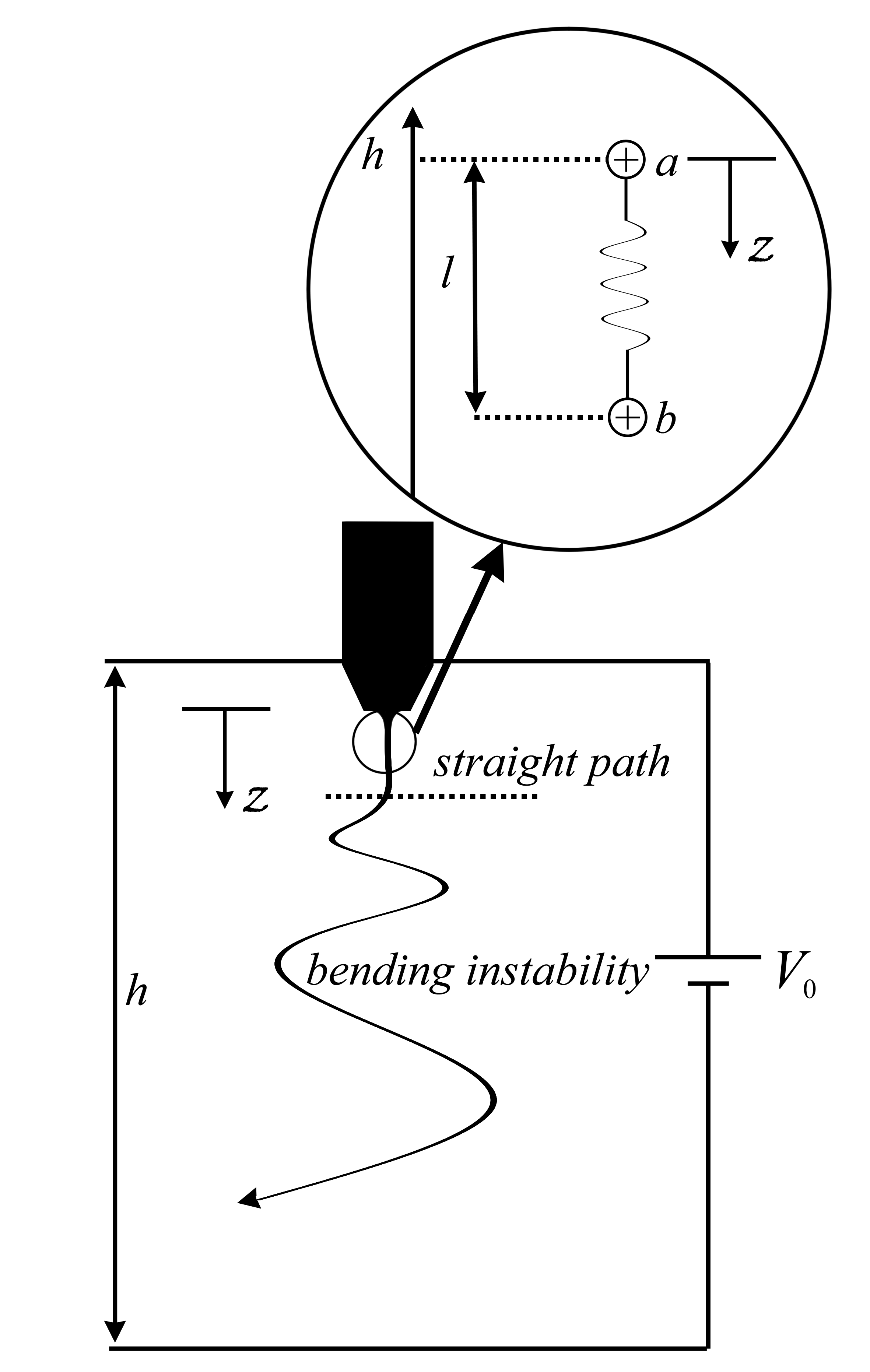
Figure 1: Schematic drawing of the electrospinning process (not in scale), showing $h$ the distance between the collector plate and the injection point (nozzle), $V_{0}$ the applied voltage between these two elements, and the $z$ reference axis whose origin is fixed at the injection point.

Let us consider a rectilinear electrified viscoelastic jet in a typical electrospinning experiment. In order to model the stretching, we represent the filament by a viscoelastic dumbbell (or dimer) with two charged beads ($a,b$) with the same mass $m$ and charge $e$ (not to be confused with the electron charge) located a distance $l$ apart (Fig. 1). One of the two beads ($a$) is held fixed to the nozzle, while the other one ($b$) is free to move under the effect of the various forces. The dumbbell $ab$ represents a schematic model for the jet. We denote by $h$ the distance of the collector plate from the injection point and by $V_{0}$ the applied voltage between them. The bead $b$ is subject to three different forces (gravity and surface tension are neglected): the external electrical field $V_{0}/h$, the Coulomb repulsive force between the two beads, and the viscoelastic force. As pointed out elsewhere [11, 15, 8], the competition between Coulomb and viscoelastic forces characterizes the early-stage of the jet elongation, while the second stage is dominated by the external electrical force, driving the fluid filament towards the collector.

The combined action of these three forces governs the elongation of the jet according to the following equation[8]:

$$m\frac{d\upsilon}{dt}=\frac{e^{2}}{l^{2}}+\frac{eV_{0}}{h}-\pi r^{2}\sigma,$$ (1)

where $\upsilon$ is the velocity of the bead $b$, $t$ the time, $r$ the cross-sectional radius of the filament, $\pi r^{2}\sigma$ the force pulling the bead $b$ back to $a$, with $\sigma$ the stress of the viscoelastic force. Assuming a viscoelastic Maxwellian liquid [7] the time evolution of the stress $\sigma$ related to the viscoelastic force is provided by the equation:

$$\frac{d\sigma}{dt}=G\frac{dl}{ldt}-\frac{G}{\mu}\sigma,$$ (2)

where $G$ is the elastic modulus, and $\mu$ the viscosity of the fluid. The velocity $\upsilon$ satisfies the kinematic relation:

$$\frac{dl}{dt}=\upsilon.$$ (3)

To include air drag effects on the dynamics of electrified jets, we add a random and dissipative term into Eq (1). Denoted $D_{\upsilon}$ the diffusion coefficient in velocity space and $\alpha$ the friction parameter, we assume that the dissipative term has the form $\alpha W$, while the random force term the form $\sqrt{2D_{\upsilon}}\eta\left(t\right)$, where $\eta\left(t\right)$ is a nowhere differentiable stochastic process with $<\eta\left(t_{1}\right)\eta\left(t_{2}\right)>=\delta\left(\left|t_{2}-t_{1}\right|\right)$, and $<\eta\left(t\right)>=0$. As a first approximation, we have taken $\alpha$ constant [11]. Adding these two force terms in Eq (1), we obtain a Langevin-like stochastic differential equation:

$$m\frac{d\upsilon}{dt}=\frac{e^{2}}{l^{2}}+\frac{eV_{0}}{h}-\pi r^{2}\sigma-m\alpha\upsilon+\sqrt{2m^{2}D_{\upsilon}}\eta\left(t\right)$$ (4)

A dependence of the dissipative term both on the velocity and on the length of nanofibers was experimentally reported [12, 14, 7], and the following empirical formula for the dissipative air drag force was proposed:

$$f_{air}=-m\alpha l^{0.905}\upsilon^{1.19},$$ (5)

where $\alpha$ denotes an empirical factor depending on the air density and kinematic viscosity of gaseous medium.

Therefore, we propose here a more comprehensive model for the Langevin-like stochastic differential equation (8.3) which takes the form:

$$m\frac{d\upsilon}{dt}=\frac{e^{2}}{l^{2}}+\frac{eV_{0}}{h}-\pi r^{2}\sigma-m\alpha l^{\,S}\upsilon^{1+P}+\sqrt{2m^{2}D_{\upsilon}}\eta\left(t\right),$$ (6)

where the parameter $P$ denotes the super-linearity of the dissipation term, and $S$ accounts for a sub-linear dependence of the dissipative term on the jet length. It is worth observing that Eq (6) reduces to Eq (4) in the limit $P,S\rightarrow 0$.

All the variables and equations are recast in a more convenient non-dimensional form [8]. To this aim, we define a length scale $L=\left(e^{2}/\pi r_{0}^{2}G\right)^{1/2}$, at which Coulomb repulsion matches the reference viscoelastic stress $G$, being $r_{0}$ the initial radius, and $\tau=\mu/G$ a relaxation time. By defining

$$\bar{t} =\frac{t}{\tau}$$ (7)

$$\bar{l} =\frac{l}{L}$$

$$\bar{W} =\upsilon\cdot\frac{\tau}{L}$$

$$\bar{\alpha} =\alpha\cdot\tau\,L^{S}\left(\frac{L}{\tau}\right)^{P}$$

$$\bar{D}_{\upsilon} =D_{\upsilon}\cdot\frac{\tau^{3}}{L^{2}}$$

and applying the conservation of the jet volume, $\pi r^{2}\,l=\pi r_{0}^{2}L$, the equations of motion in terms of non-dimensional (barred) variables take the following form:

$$\frac{d\bar{l}}{d\bar{t}} =\bar{W}$$ (8a)

$$\frac{d\bar{\sigma}}{d\bar{t}} =\frac{\bar{W}}{\bar{l}}-\bar{\sigma}$$ (8b)

$$\frac{d\bar{W}}{d\bar{t}} =\frac{Q}{\bar{l}^{2}}+V-F_{ve}\frac{\bar{\sigma}}{\bar{l}}-\bar{\alpha}\bar{l}^{\,S}\bar{W}^{1+P}+\sqrt{2\bar{D}_{\upsilon}}\eta\left(\bar{t}\right)$$ (8c)

The dimensionless groups are given by:

$$Q =\frac{e^{2}\mu^{2}}{L^{3}mG^{2}}$$ (9)

$$V =\frac{eV_{0}\mu^{2}}{hLmG^{2}}$$

$$F_{ve} =\frac{\pi r_{0}^{2}\mu^{2}}{mLG}$$

The three group measure the strength of Coulomb interactions, external field and viscoleastic forces in units of the inertial force $md\upsilon/dt$, respectively. In these units, $F_{ve}=Q$, so that we are left with four independent parameters (considering also $\bar{\alpha}$ and $\bar{D}_{\upsilon}$).

2.1 Numerical integration

The equations of motion equations are discretised on a uniform sequence $t_{i}=t_{0}+i\Delta t$, $i=1,\ldots,n_{steps}$. At each time step, we first integrate the stochastic Eq (8c) using the explicit “strong” order scheme proposed by E. Platen [17, 18], whereof the order of “strong” convergence was evaluated in literature equal to $1.5$.

The Platen scheme delivers:

$$Y_{t+\varDelta t}^{k}= Y_{t}^{k}+b^{k}\Delta\Omega+\frac{1}{2\left(\Delta t\right)^{\nicefrac{{1}}{{2}}}}\left[a^{k}\left(\vec{\boldsymbol{\Upsilon}}_{+}\right)-a^{k}\left(\vec{\boldsymbol{\Upsilon}}_{-}\right)\right]\Delta\varPsi$$ (10)

$$+\frac{1}{4}\left[a^{k}\left(\vec{\boldsymbol{\Upsilon}}_{+}\right)+2a^{k}+a^{k}\left(\vec{\boldsymbol{\Upsilon}}_{-}\right)\right]\Delta t$$

with $Y_{t}^{k}$ denoting the approximation for the k-th component of a generic vector $\vec{\textbf{X}}$ whereof the time derivative is $d\vec{\textbf{X}}/dt=\vec{\textbf{a}}\left(t,X^{1},\ldots,X^{d}\right)+\vec{\textbf{b}}\,d\Omega$, denoting $\Omega\left(t\right)$ a Wiener process. Here, the vector supporting values $\vec{\boldsymbol{\Upsilon}}_{\pm}$ are

$$\vec{\boldsymbol{\Upsilon}}_{\pm}=\vec{\textbf{Y}}_{t}+\vec{\textbf{a}}\Delta t\pm\vec{\textbf{b}}\left(\Delta t\right)^{\nicefrac{{1}}{{2}}},$$ (11)

and $\Delta\Omega$ and $\Delta\varPsi$ are normally distributed random variables related to two independent $N\left(0,1\right)$ standard Gaussian distributed random variables $U_{1}$ and $U_{2}$ via the linear transformation:

$$\Delta\Omega=U_{1}\left(\Delta t\right)^{\nicefrac{{1}}{{2}}}\qquad\Delta\varPsi=\frac{1}{2}\left(\Delta t\right)^{\nicefrac{{3}}{{2}}}\left(U_{1}+\frac{1}{\sqrt{3}}U_{2}\right).$$ (12)

Note that for $\left|\vec{\textbf{b}}\right|=0$ the Platen scheme reduces to the second-order Runge-Kutta scheme. Finally, the remaining Eqs (8a) and (8b) are integrated via a second order Runge-Kutta scheme with the $\bar{W}_{i+1}$ value previously obtained via the Platen scheme.

3 Results and Discussion

We investigate different regimes of electrified jets associated with the Eqs (6), with special focus on metastable states and asymptotic behavior. As a reference case, we consider the typical values of $Q=12$ and $V=2$, already investigated in previous works[15, 8]. All simulations start from the same initial conditions: $\bar{l}=1$, $\bar{\sigma}=0$ and $\bar{W}=0$. Note that for reference parameters developed by experimental results[8] the typical values of length scale $L$ and relaxation time $\tau$ are $3.19\>\text{\text{mm}}$, and $10^{-2}\,\text{s}$, respectively.

3.1 Parameter setup and asymptotes

First, we study the deterministic case, by imposing $\bar{\alpha}=\bar{D}_{\upsilon}=0$. We integrate in time forward and backward Eqs (8) in the interval $\bar{t}_{a}=0$ and $\bar{t}_{b}=5$ at different values of time-step $\Delta\bar{t}$ in order to assess a suitable value for the specific case under investigation. Exploiting the time reversibility, we measured an average absolute error $\Delta\bar{l}=\left|\bar{l}_{2n_{steps}}-\bar{l}_{0}\right|$ lower than $10^{-12}$ with time step $\Delta\bar{t}=10^{-2}$. Therefore, we take a time step $\Delta\bar{t}=10^{-3}$, as a conservative choice for the specific case under investigation.

We next discuss the elongation of the jet under stochastic perturbation. To estimate the parameters $\bar{\alpha}$, $S$ and $P$, we consider the empirical formula Eq (5) for the dissipative air drag force[12, 14, 7]. For typical air density, kinematic viscosity of air gaseous medium and jet mass (assumed constant), we obtain a $\bar{\alpha}\sim 0.5$ (with $\tau=10^{-2}\,\text{s}$), while the parameters $S$ and $P$ are set equal to $0.905$ and $0.19$, respectively. For all the investigated cases, we adopt for the sake of simplicity the value $\bar{D}_{\upsilon}=\bar{\alpha}$. In order to accumulate sufficient statistics, we have run $10000$ independent trajectories for each different case under investigation. Thence, we compute the time dependent mean value of our observables along the dynamics.

We integrate the Eqs (8c) for three different cases: in the first, we set $\bar{\alpha}=0$, $S=0$ and $P=0$ (deterministic case); in the second $\bar{\alpha}=0.5$, $S=0$ and $P=0$ (linear Langevin); for the third case (non-linear Langevin) $\bar{\alpha}=0.5$ while and $S=0.905$ and $P=0.19$, respectively.

Three basic time-asymptotic regimes can be identified:

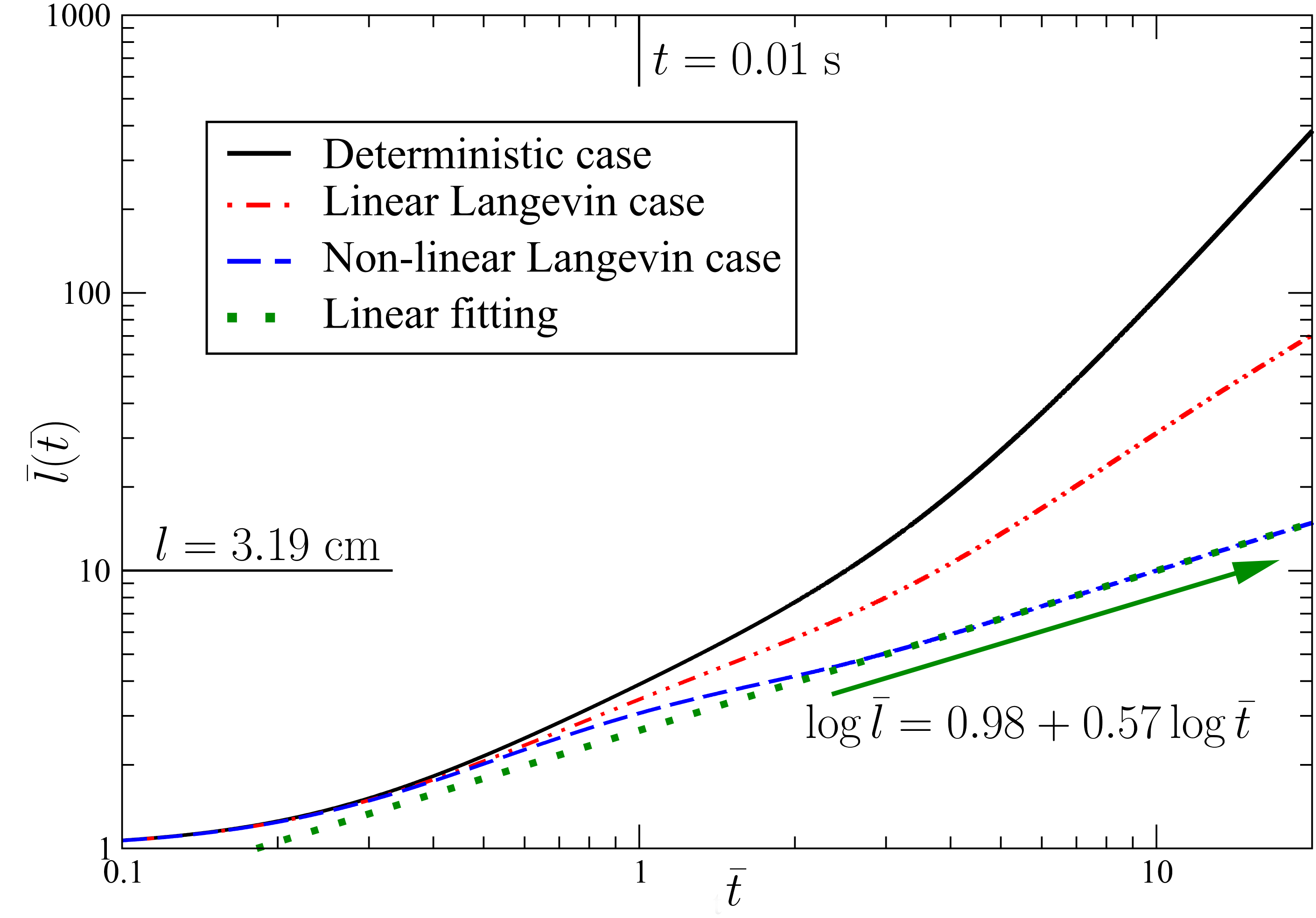
Figure 2: Time evolution of the jet elongation $\bar{l}\left(\bar{t}\right)$ for three different cases: 1) Deterministic: $\bar{\alpha}=0$, $S=0$ and $P=0$ in black continuous line; 2) Linear Langevin: $\bar{\alpha}=0.5$, $S=0$ and $P=0$ in red dashed line; 3) Non-linear Langevin: $\bar{\alpha}=0.5$, $S=0.905$ and $P=0.19$ in blue dotted-dashed line. In green dotted line we report the linear fitting (in log-log scale) for the Non-linear Langevin case with slope equal to the expected value $\nicefrac{{4}}{{7}}$. The horizontal line on the left side corresponds to the physical length $\l=3.19$ cm.

i) Deterministic: $\bar{W}\propto\bar{t}^{2}$, $\bar{l}\propto\bar{t}^{2}$. This is the free-fall regime driven by the external voltage, once every other force is extinguished (see Fig 2).

ii) Stochastic, Linear Dissipation: $\bar{W}\propto const$, $\bar{l}\propto\bar{t}$. This is the ballistic regime resulting from the balance between the external field and linear dissipation. Asymptotically, the jet moves at a constant speed, like electrons in a linear host media.

iii) Stochastic, Non-linear: $\bar{l}\propto\bar{t}^{4/7}$, $\bar{W}\propto\bar{t}^{-3/7}$. This is the regime resulting from the balance between the external field and non-linear dissipation with $S=0.905$ and $P=0.19$. Note that, even though these exponents are close to the case of standard diffusion, they result from a very different process, namely a constant force against a drag growing with the filament length. It is interesting to notice that the filament length is still unbounded in the limit $t\to\infty$ (see Fig 2), but much slower than the ballistic case associated with linear dissipation. We emphasize that these asymptotic regimes, although important for a qualitative analysis of the process, bear limited practical interest since, in the long-term, the jet undergoes a bending instability which cannot be described by the present one-dimensional model. The one-dimensional model is however very useful to discuss the early-stage of the evolution and incipient onset of the instability. In Fig 3, we report the velocity $\bar{W}\left(\bar{t}\right)$ versus time for the three cases above.

3.2 Deterministic case: no dissipation

In the deterministic case, we identify two sequential stages in the elongation process (denoted $A$ and $B$ in Fig 3). In the first regime, we observe a small increase of $\bar{W}\left(\bar{t}\right)$, which rises up to achieve a quasi stationary point denoted by $\bar{t}_{*}$, where the viscoelastic force ${\displaystyle\frac{F_{ve}\bar{\sigma}\left(\bar{t}_{*}\right)}{\bar{l}\left(\bar{t}_{*}\right)}}$ balances the sum of the two force terms ${\displaystyle\frac{Q}{\bar{l}\left(\bar{t}_{*}\right)^{2}}}$ and $V$, providing a zero total force. Subsequently, after about $20-40$ ms, the velocity attains a near-linearly increasing trend, close to the time-asymptotic solution discussed above (see also Ref [15]). Note that the instant $\bar{t}_{*}$ corresponds to the lower limit of the derivative $\partial\bar{W}\left(\bar{t}\right)/\partial\bar{t}$, and discerns the two stages of the dynamics, regime $A$ characterized by the competition between Coulomb and viscoelasticity, and regime $B$, characterized by the sole action of the external field.

3.3 Stochastic case: linear dissipation

Once linear dissipation is included, the jet elongation suffers an additional slow down, leading to a decrease of the velocity after the early peak driven by Coulomb forces. This leads to a local minimum at $\bar{t}_{**}$ with no counterpart in the deterministic case, as already discussed in Ref [11]. We observe that the time occurrence $\bar{t}_{*}$ of the peak is anticipated by the air drag, an the corresponding velocity slightly decreased. Subsequently, in the regime $B$ the velocity attains its asymptotic value (see Fig 3).

3.4 Stochastic case: non-linear dissipation

In the third case (non-linear Langevin), we observe that the non-linearity of the dissipative term largely alters the time evolution of velocity. In particular, it leads to just one quasi stationary point. Furthermore, the velocity $\bar{W}\left(\bar{t}\right)$ appears to tend asymptotically to zero, as it pertains to its asymptotic regime

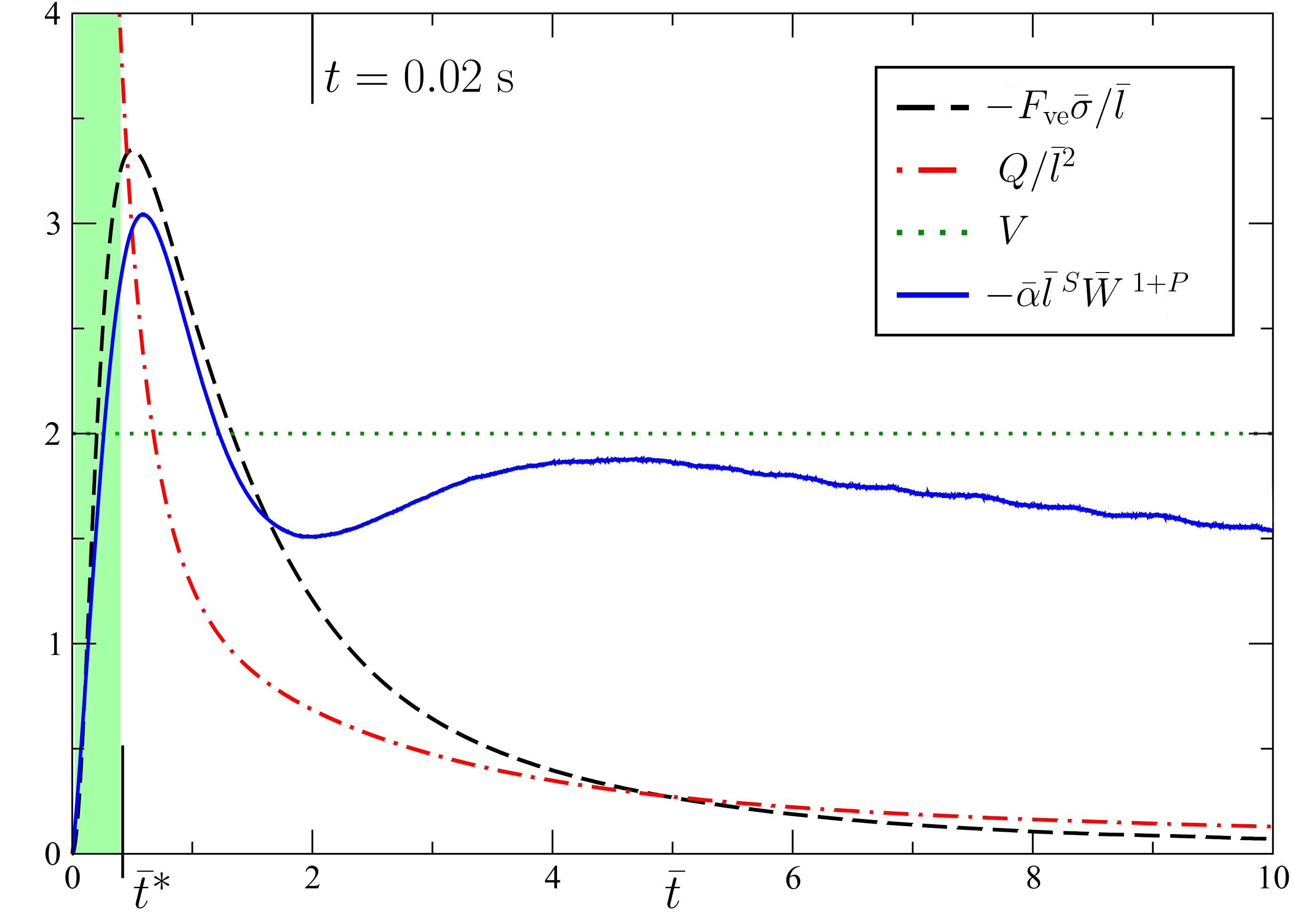
Figure 4: Time evolution of the four force terms versus time $\bar{t}$: $-{\displaystyle\bar{\alpha}\bar{l}^{\,S}\bar{W}^{1+P}}$ (continuous line), $-{\displaystyle\frac{F_{ve}\bar{\sigma}}{\bar{l}}}$ (dashed line), $V$ (dotted line), and ${\displaystyle\frac{Q}{\bar{l}^{2}}}$ (dashed-dotted line) for the non-linear Langevin case $\bar{\alpha}=0.5$. The quasi-stationary point $\bar{t}^{*}=0.4$ is highlighted. The viscoelastic force $-{\displaystyle\frac{F_{ve}\bar{\sigma}}{\bar{l}}}$ peaks at about $\bar{t}=0.5$. Subsequently, the force terms ${\displaystyle-\frac{F_{ve}\bar{\sigma}}{\bar{l}}}$ and ${\displaystyle\frac{Q}{\bar{l}^{2}}}$ decay to zero, while the term $-\bar{\alpha}\bar{l}^{S}\bar{W}^{1+P}$ and the external electrical field $V$ govern the jet dynamics.

We next examine the force terms, as shown in Fig 4. First, the Coulombic term ${\displaystyle\frac{Q}{\bar{l}\left(\bar{t}\right)^{2}}}$ decays rapidly so that it plays no role in regime $B$. The early-stage of the dynamics is characterized by the terms ${\displaystyle\frac{F_{ve}\bar{\sigma}\left(\bar{t}\right)}{\bar{l}\left(\bar{t}\right)}}$ and $\bar{\alpha}\bar{l}^{\,S}\bar{W}^{1+P}$, which increase as consequence of the jet stretching due to the external electric field. This early-stage comes to the quasi stationary point at time $\bar{t}_{*}$, where ${\displaystyle\frac{F_{ve}\bar{\sigma}\left(\bar{t}\right)}{\bar{l}\left(\bar{t}\right)}}$ and $\bar{\alpha}\bar{l}^{\,S}\bar{W}^{1+P}$ conspire to balance the external drive $V$.

After the instant $\bar{t}_{*}$, the term $\bar{\alpha}\bar{l}^{\,S}\bar{W}^{1+P}$ becomes larger in magnitude, leading to a decrease of the velocity $\bar{W}$, due to the dissipative and viscoelastic terms (see Fig 3). At the same time, the term ${\displaystyle\frac{F_{ve}\bar{\sigma}\left(\bar{t}\right)}{\bar{l}\left(\bar{t}\right)}}$ starts to decay, and the jet dynamics is governed only by the remaining opposite terms $V$ and $\bar{\alpha}\bar{l}^{\,S}\bar{W}^{1+P}$. Since dissipation grows quasi-linearly with the jet elongation, the velocity goes to zero in the time asymptotic limit.

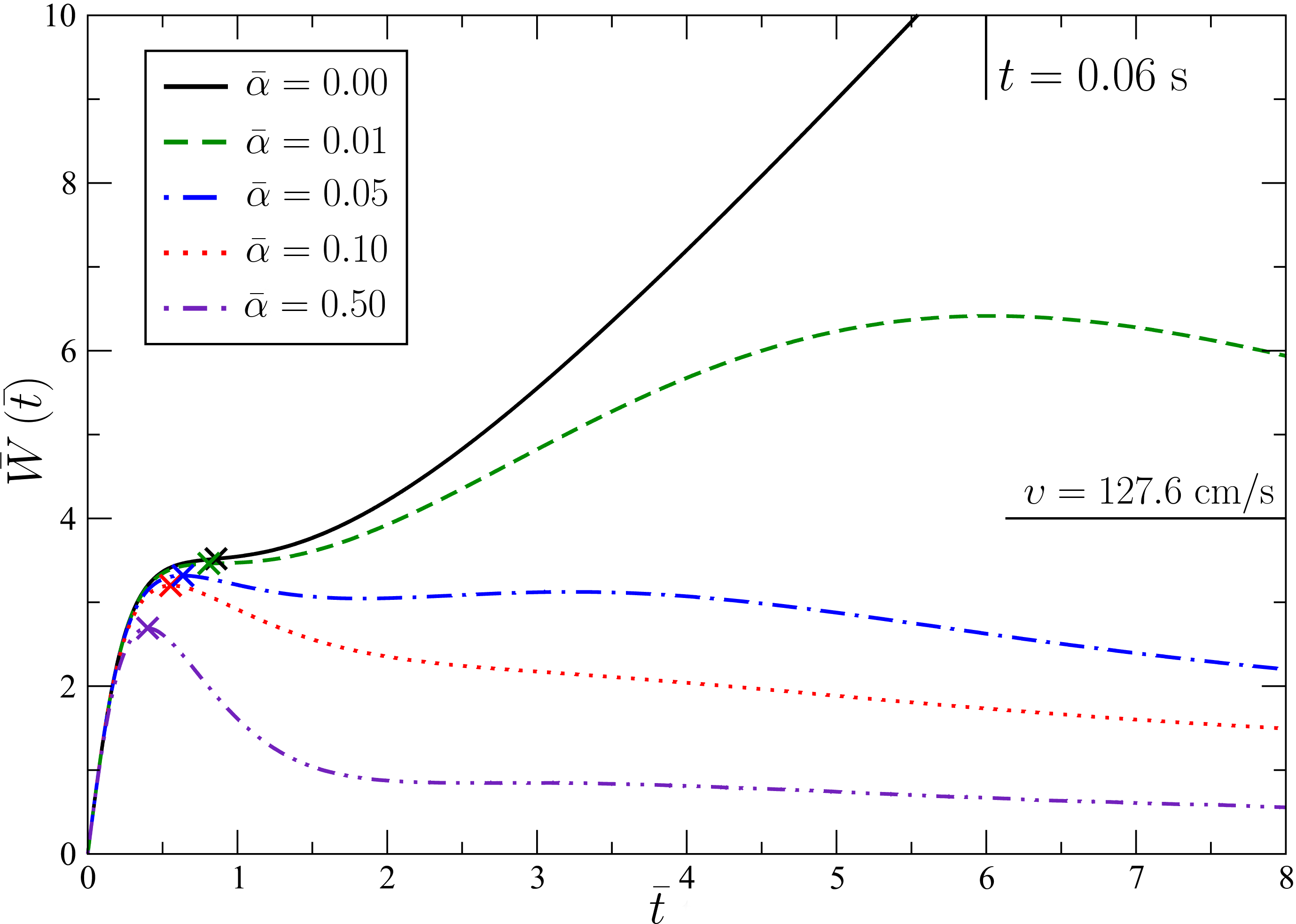
Figure 5: Time evolution of the velocity $\bar{W}\left(\bar{t}\right)$ for different values of $\bar{\alpha}$. From top to bottom curves: $\bar{\alpha}$ = 0 (continuous line), 0.01 (dashed line), 0.05 (dashed-dotted line), and 0.1 (dotted line), and 0.5 (dashed-dotted-dotted line), keeping $\bar{D}_{\upsilon}=\bar{\alpha}$ for all the cases. The quasi-stationary points are denoted by a star symbol. As expected, increasing the drag coefficient entails a substantial reduction of the filament velocity. The horizontal line on the right side corresponds to the physical speed $\upsilon=127.6$ cm/s.

Next, we investigate the elongation of jet under stochastic perturbation modelled by the non-linear Langevin equation for different values of $\bar{\alpha}$, keeping the condition $\bar{D}_{\upsilon}=\bar{\alpha}$. In particular, we explore the way that the position of $\bar{t}_{*}$ is altered by the dissipative-perturbing force $-\bar{\alpha}\bar{l}^{\,S}\bar{W}^{1+P}+\sqrt{2\bar{D}_{\upsilon}}\eta\left(\bar{t}\right)$ in Eq (8c). In Fig 5, we report the time evolution of the velocity $\bar{W}\left(\bar{t}\right)$ for different $\bar{\alpha}$. For all investigated regimes we observe a quasi stationary point at time $\bar{t}_{*}$, which decreases by increasing the term $\bar{\alpha}$ (see Tab 1).

The straight path of the electrified jet is described by the observable $\bar{l}\left(\bar{t}_{*}\right)$, which is seen to decrease by increasing $\bar{\alpha}$ (Fig 6). Useful hints for the optimal design of the electrospinning processes, resulting from deeper insights into the early-stage dynamics of the jet can be numerous, including the possibility of better controlling the subsequent development of three-dimensional instabilities, and consequently, the diameter and morphology of collected nanostructures, as well as the assembly and positions of nanofibers impinging onto the collector. A better control of these nanofabrication processes could therefore entail the identification and tailoring of air drag mechanisms, which can eventually be induced by a proper designed of gas-injecting systems nearby the spinneret.

4 Conclusions

Summarizing, we have investigated the flow of charged viscoelastic fluids in the presence of stationary stochastic perturbations. A Brownian term has been used to model the effects of a perturbing force on the stretching properties of electrically charged jets, providing significant qualitative new insights. We demonstrated that the non-linear dependence of the dissipative term on the geometry of the electrospun polymer provides important effects that cannot be properly modelled by a linear Langevin-like stochastic differential equation. We also observed that the air drag force significantly affects the dynamics of the electrospinning process, leading to a time-asymptotic vanishing velocity of the jet. Furthermore, a reduction of the linear extension of the jet is observed in the early-stage by increasing the dissipative force term. These results may contribute to the optimal set-up of the experimental conditions, so as to enhance the efficiency of the process and the quality of the electrospun fibers. These may include, among others, environmental vibrations and resulting micro-vorticity patterns.

Tables

$\bar{\alpha}$	$\bar{t}_{*}$	$\bar{l}\left(\bar{t}_{*}\right)$	$\bar{\sigma}\left(\bar{t}_{*}\right)$	$\bar{W}\left(\bar{t}_{*}\right)$
0	0.86	3.39	0.81	3.52
0.01	0.81	3.21	0.80	3.46
0.05	0.64	2.58	0.71	3.32
0.1	0.55	2.29	0.65	3.20
0.5	0.40	1.75	0.47	2.69

Table 1: Values of the dimensionless variables length $\bar{l}$, stress $\bar{\sigma}$ and velocity $\bar{W}$ at the quasi-stationary points $\bar{t}_{*}$ computed for different values of $\bar{\alpha}$. To be noted the decrease of $\bar{t}_{*}$ at increasing $\bar{\alpha}$ .Furthermore, we stress the decrease of the lenght $\bar{l}\left(\bar{t}_{*}\right)$ (see Fig. 6), proving that the initial stage of the elongation process contracts as a consequence of the uniaxial perturbation.

Figures

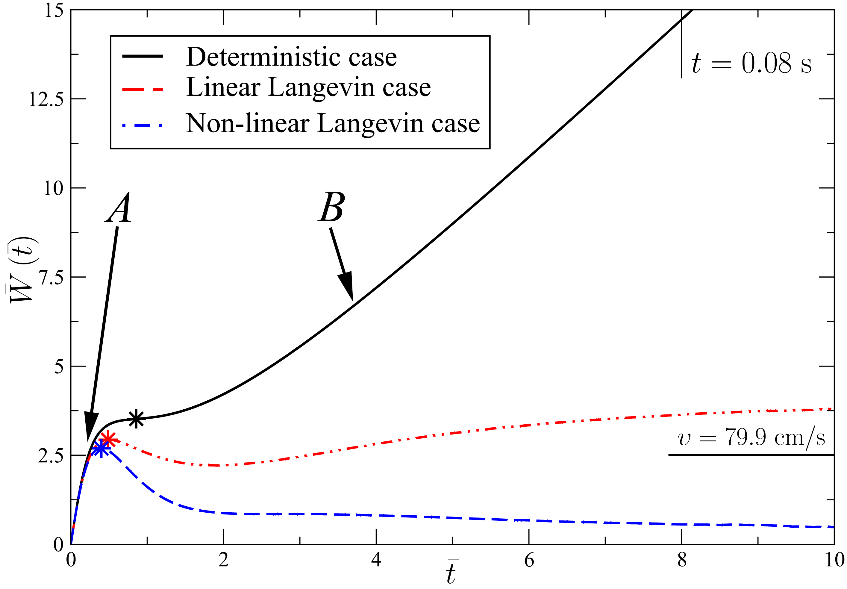
Figure 3: Time evolution of the velocity $\bar{W}\left(\bar{t}\right)$ for three different cases: 1) Deterministic: $\bar{\alpha}=0$, $S=0$ and $P=0$ in black continuous line; 2) Linear Langevin: $\bar{\alpha}=0.5$, $S=0$ and $P=0$ in red dashed line; 3) Non-linear Langevin: $\bar{\alpha}=0.5$, $S=0.905$ and $P=0.19$ in blue dotted-dashed line. Two stages of the elongation process are identified: an early transient ($A$), which comes to a quasi stationary point (denoted by a star symbol) and a later stage ($B$) controlled by the competition between the external field and air dissipation. The figure highlights the major role played by dissipation on the long-term evolution of the system, which is from free-fall acceleration to a constant velocity regime. As expected, the super-linear dissipation enhances the drag effect, leading to a further reduction of the time-asymptotic speed. The horizontal line on the right side corresponds to the physical speed $\upsilon=79.9$ cm/s.

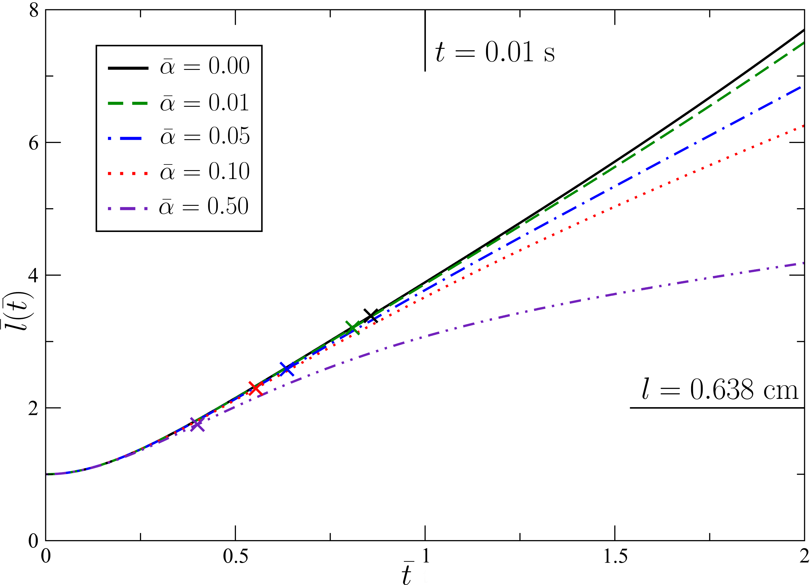
Figure 6: Time evolution of the jet elongation $\bar{l}\left(\bar{t}\right)$ for different values of $\bar{\alpha}$: $0$ (continuous line), $0.01$ (dashed line), $0.05$ (dashed-dotted line), and $0.1$ (dotted line), and $0.5$ (dashed-dotted-dotted line), keeping $\bar{D}_{\upsilon}=\bar{\alpha}$ for all the cases. The quasi-stationary points are depicted as star symbol. The horizontal line on the right side corresponds to the physical length $l=0.638$ cm.

Supplemental Information

In this paper, we use a recast form of the empirical formula for the air drag force $f_{air}$ usually found in literature. Here, we provide few details on our revised expression. The original empirical formula for the air drag force $f_{air}$ is

$$f_{air}=l\cdot 0.65\pi r\rho_{air}\upsilon^{2}\left(\frac{2\upsilon r}{\nu_{air}}\right)^{-0.81},$$ (1)

where we consider $l$ as the distance between the beads labeled $i$ and $i-1$ , $r$ the cross-sectional radius of the filament, $\upsilon$ is the velocity of the $i-th$ bead, $\rho_{a}$ is the air density, and $\nu_{a}$ is the air kinematic viscosity.

We rearrange the Eq as

$$f_{air}=l\cdot 0.65\pi\rho_{air}\left(\frac{2}{\nu_{air}}\right)^{-0.81}r^{0.19}\upsilon^{1.19}.$$ (2)

Assuming a constant volume of the jet $\pi r^{2}l=\pi r_{0}^{2}L$, so that $r=r_{0}\sqrt{L/l}$ with $L$ and $r_{0}$ respectively the length and the radius of the jet segment between the beads $i$ and $i-1$ at the nozzle before the stretching, we obtain

$$f_{air}=0.65\pi\rho_{air}\left(\frac{2}{\nu_{air}}\right)^{-0.81}l\left(r_{0}L^{0.5}l^{-0.5}\right)^{0.19}\upsilon^{1.19}.$$ (3)

Thus, we can write

$$f_{air}=\left[0.65\pi\rho_{air}\left(\frac{2}{\nu_{air}}\right)^{-0.81}L^{0.095}r_{0}^{0.19}\right]l^{0.905}\upsilon^{1.19}.$$ (4)

If we write $f_{air}$ as

$$f_{air}=m_{i}\alpha l^{0.905}\upsilon^{1+0.19},$$ (5)

denoting $m_{i}$ the mass of the bead $i$, we obtain an equivalent formula for the air drag force with the dissipative coefficient $\alpha$ equal to

$$\alpha=0.65\pi\rho_{air}\left(\frac{2}{\nu_{air}}\right)^{-0.81}\frac{L^{0.095}r_{0}^{0.19}}{m_{i}}.$$ (6)

References

- [1] Marc Baus and JP Hansen. Statistical mechanics of simple coulomb systems. Physics Reports, 59:1–94, 1980.
- [2] J.P. Hansen. Structure and dynamics of charged fluids. In NormanH. March, RobertA. Street, and MarioP. Tosi, editors, Amorphous Solids and the Liquid State, Physics of Solids and Liquids, pages 229–280. Springer US, 1985.
- [3] Lydéric Bocquet and Jean-Pierre Hansen. Dynamics of colloidal systems: Beyond the stochastic approach. In John Karkheck, editor, Dynamics: Models and Kinetic Methods for Non-equilibrium Many Body Systems, volume 371 of NATO Science Series, pages 1–16. Springer Netherlands, 2002.
- [4] Antoine Carof, Virginie Marry, Mathieu Salanne, Jean-Pierre Hansen, Pierre Turq, and Benjamin Rotenberg. Coarse graining the dynamics of nano-confined solutes: the case of ions in clays. Molecular Simulation, 40(1-3):237–244, 2014.
- [5] Geoffrey Taylor. Electrically driven jets. Proceedings of the Royal Society of London. A. Mathematical and Physical Sciences, 313(1515):453–475, 1969.
- [6] D. Pisignano. Polymer Nanofibers: Building Blocks for Nanotechnology. Royal Society of Chemistry, 2013.
- [7] Alexander L Yarin, Behnam Pourdeyhimi, and Seeram Ramakrishna. Fundamentals and Applications of Micro and Nanofibers. Cambridge University Press, 2014.
- [8] Darrell H Reneker, Alexander L Yarin, Hao Fong, and Sureeporn Koombhongse. Bending instability of electrically charged liquid jets of polymer solutions in electrospinning. Journal of Applied physics, 87(9):4531–4547, 2000.
- [9] L. Persano, A. Camposeo, C. Tekmen, D. Pisignano, Industrial upscaling of electrospinning and applications of polymer nanofibers: a review, Macromolecular Materials and Engineering 298 (5) (2013) 504–520.
- [10] Ivan Coluzza, Dario Pisignano, Daniele Gentili, Giuseppe Pontrelli, and Sauro Succi. Ultrathin fibers from electrospinning experiments under driven fast-oscillating perturbations. Physical Review Applied, 2(5):054011, 2014.
- [11] Marco Lauricella, Giuseppe Pontrelli, Ivan Coluzza, Dario Pisignano, and Sauro Succi. Different regimes of the uniaxial elongation of electrically charged viscoelastic jets due to dissipative air drag. Submitted to Mechanics Research Communications, 2014.
- [12] A. Ziabicki and H. Kawai. High-Speed Fiber Spinning: Science and Engineering Aspects. Krieger Publishing Co, 1991.
- [13] RA Antonia, BR Satyaprakash, and AKMF Hussain. Measurements of dissipation rate and some other characteristics of turbulent plane and circular jets. Physics of Fluids (1958-1988), 23(4):695–700, 1980.
- [14] Suman Sinha-Ray, Alexander L Yarin, and Behnam Pourdeyhimi. Meltblowing: I-basic physical mechanisms and threadline model. Journal of Applied Physics, 108(3):034912, 2010.
- [15] Giuseppe Pontrelli, Daniele Gentili, Ivan Coluzza, Dario Pisignano, and Sauro Succi. Effects of non-linear rheology on the electrospinning process: a model study. Mechanics Research Communications, 61:41–46, 2014.
- [16] Daniel Thomas Gillespie and Effrosyni Seitaridou. Simple Brownian Diffusion: An Introduction to the Standard Theoretical Models. Oxford University Press, 2012.
- [17] E Platen. Derivative free numerical methods for stochastic differential equations. In Stochastic Differential Systems, pages 187–193. Springer, 1987.
- [18] Peter E Kloeden and Eckhard Platen. Numerical solution of stochastic differential equations, volume 23. Springer, 1992.