On the Performance of Turbo Signal Recovery
with Partial DFT Sensing Matrices

Abstract

This letter is on the performance of the turbo signal recovery (TSR) algorithm for partial discrete Fourier transform (DFT) matrices based compressed sensing. Based on state evolution analysis, we prove that TSR with a partial DFT sensing matrix outperforms the well-known approximate message passing (AMP) algorithm with an independent identically distributed (IID) sensing matrix.

I Introduction

The approximate message passing (AMP) algorithm [1, 2, 3, 4, 5, 6, 7, 8, 9] is an efficient signal recovery method for compressed sensing. Its convergence is asymptotically guaranteed for sensing matrices with independent identically distributed (IID) entries using the state evolution technique [1, 2]. The fixed points of the state evolution for AMP include the optimal minimum mean squared-error estimation (MMSE) solution [11, 12, 13]. This indicates that AMP is asymptotically optimal when the state evolution equation has a unique solution.

AMP can also be applied to problems involving non-IID sensing matrices [14, 15]. However, the state evolution technique is not directly applicable in this case.

Alternative techniques have been developed for non-IID sensing matrices [16, 17, 18]. It has been observed that these techniques with partial discrete Fourier transform (DFT) matrices [19, 20, 21, 22] can outperform AMP with IID sensing matrices under proper normalization conditions. The comparisons in [16, 17, 18] were based on simulations and no analytical results have been reported so far.

This letter is on the performance analysis of turbo signal recovery (TSR) with a partial DFT sensing matrix [18]. We prove based on state evolution that TSR with a partial DFT matrix (TSR-DFT) outperforms AMP with an IID Gaussian matrix (AMP-IID). Since the state evolution technique for AMP does not apply to problems involving a partial DFT matrix (AMP-DFT), we compare TSR-DFT and AMP-DFT through simulations. Our numerical results suggest that TSR-DFT converges faster than AMP-DFT.

II Problem Description

Consider the following linear system:

$$\bm{y}=\bm{F}_{\mathrm{partial}}\bm{x}+\bm{n}$$ (1)

where $\bm{x}\in\mathbb{C}^{N\times 1}$ is a sparse signal, $\bm{n}\sim\mathcal{CN}(\mathbf{0},\sigma^{2}\bm{I})$ the additive white Gaussian noise (AWGN) and $\bm{F}_{\mathrm{partial}}\in\mathbb{C}^{M\times N}$ ($M<N$) a partial DFT matrix consisting of $M$ randomly selected rows of the normalized DFT matrix $\bm{F}$. The $(m,n)$th entry of $\bm{F}$ is given by $\frac{1}{\sqrt{N}}\exp\big{(}-\mathrm{j}\frac{2\pi(m-1)(n-1)}{N}\big{)}$.

We assume that the entries of $\bm{x}$ are IID. The $j$th entry $x_{j}$ follows the Bernoulli-Gaussian distribution [3]

$$x_{j}\sim\begin{cases}0&\text{probability}=1-\lambda,\\ \mathcal{CN}(0,\lambda^{-1})&\text{probability}=\lambda.\end{cases}$$ (2)

By this definition, $\mathrm{E}[|x_{j}|^{2}]=1$. Here $\lambda$ determines the sparsity of the system. The partial DFT matrix can be rewritten as

$$\bm{F}_{\mathrm{partial}}=\bm{SF},$$ (3)

where $\bm{S}$ consists of $M$ randomly selected rows of the identity matrix. We define the following auxiliary vector:

$$\bm{z}=\bm{Fx}.$$ (4)

Combining (1) and (4), we have

$$\bm{y}=\bm{S}\bm{z}+\bm{n}.$$ (5)

Our objective is to recover $\bm{x}$ based on $\bm{y}$ under the assumption that $\bm{x}$ is sparse with $\lambda<1$.

Figure 1: Functional diagram of a standard turbo processor.

III Turbo Signal Recovery

Figure 2: Functional diagram of the turbo signal recovery (TSR) algorithm [18].“ext” represents extrinsic message computation.

III-A Standard Turbo Processor

Fig. 1 shows a standard turbo-type signal processor [23] for the problem under consideration. The related operations can be grouped into two modules labeled as A and B. Module A is a linear minimum mean-squared error (LMMSE) estimator [24] of $\bm{x}$ based on (1) without the sparsity information, while module B estimates $\bm{z}$ based on the sparsity information in (2). The two modules work iteratively.

Since LMMSE estimation is standard, we will focus on module B. The input of module B, denoted by $\bm{x}_{B}^{pri}$ (see Fig. 1), is modeled as [18]

$$\bm{x}_{B}^{pri}=\bm{x}+\bm{w},$$ (6)

where $\bm{w}$ is IID Gaussian and independent of $\bm{x}$. For each $j$, the sparsity combiner produces the a posteriori mean $\mathrm{E}_{x_{j}}\{x_{j}|\bm{x}_{B}^{pri}\}$ based on the AWGN assumption in (6) and the sparsity constraint in (2). Let “_∼j” denote indices excluding $j$. The extrinsic mean is defined as $\mathrm{E}_{x_{j}}\{x_{j}|\bm{x}_{B,\sim j}^{pri}\}$. Since $\bm{x}_{B}^{pri}$ is assumed to be an AWGN observation of $\bm{x}$, the extrinsic mean will not improve during the iterative process based on Fig. 1. The problem here is that the sparsity constraint is symbol-by-symbol and so $\bm{x}_{B,\sim j}^{pri}$ does not provide any information about $x_{j}$. For details, see [18].

III-B Turbo Signal Recovery

The TSR algorithm proposed in [18] is listed in Algorithm 1 and graphically illustrated in Fig. 2. The TSR algorithm computes the extrinsic message of $\bm{z}$ (instead of $\bm{x}$) for module B. This avoids the above mentioned problem for the standard turbo processor. Refer to [18] for more details.
 
Algorithm 1: Turbo Signal Recovery (TSR)
 
Initialization: $\bm{z}^{pri}_{A}\leftarrow\mathbf{0}$, and $v^{pri}_{A}\leftarrow 1$.
for $iteration=1:T_{max}$
1) Update

$$\bm{x}_{A}^{pri}\leftarrow\bm{F}^{\mathrm{H}}\bm{z}_{A}^{pri}.$$ (7)

2) Compute the a posteriori mean/variance of $\bm{z}$

$${\bm{z}}_{A}^{post} \leftarrow{\bm{z}}_{A}^{pri}+\frac{{v_{A}^{pri}}}{{v_{A}^{pri}+\sigma^{2}}}{\bm{S}}^{\rm{H}}\left({{\bm{y}}-{\bm{Sz}}_{A}^{pri}}\right),$$ (8a)

$$v_{A,j}^{post} \leftarrow v_{A}^{pri}-\frac{{\left({v_{A}^{pri}}\right)^{2}}}{{v_{A}^{pri}+\sigma^{2}}}\left({{\bm{S}}^{\rm{H}}{\bm{S}}}\right)_{\left({j,j}\right)},$$ (8b)

where $\left(\bm{S}^{\mathrm{H}}\bm{S}\right)_{(j,j)}$ denotes the $(j,j)$th entry of $\bm{S}^{\mathrm{H}}\bm{S}$.
3) Compute the a posteriori mean/variance of $\bm{x}$

$${\bm{x}}_{A}^{post} \leftarrow{\bm{F}}^{\rm{H}}{\bm{z}}_{A}^{post},$$ (9a)

$$v_{A}^{post} \leftarrow\frac{1}{N}\sum\limits_{j=1}^{N}{v_{A,j}^{post}}=v_{A}^{pri}-\frac{M}{N}\frac{{\left({v_{A}^{pri}}\right)^{2}}}{{v_{A}^{pri}+\sigma^{2}}}.$$ (9b)

4) Compute the extrinsic mean/variance of $\bm{x}$

$$v_{B}^{pri} \leftarrow v_{A}^{ext}\leftarrow\left({\frac{1}{{v_{A}^{post}}}-\frac{1}{{v_{A}^{pri}}}}\right)^{-1},$$ (10a)

$${\bm{x}}_{B}^{pri} \leftarrow{\bm{x}}_{A}^{ext}\leftarrow v_{A}^{ext}\left({\frac{{{\bm{x}}_{A}^{post}}}{{v_{A}^{post}}}-\frac{{{\bm{x}}_{A}^{pri}}}{{v_{A}^{pri}}}}\right).$$ (10b)

5) Update

$${\bm{z}}_{B}^{pri}\leftarrow{\bm{Fx}}_{B}^{pri}.$$ (11)

6) Compute the a posteriori mean/variance of each $x_{j}$

$$x_{B,j}^{post} \leftarrow{\rm{E}}_{x_{j}}\left\{{x_{j}|x_{B,j}^{pri}}\right\}{\rm{,}}$$ (12a)

$$v_{B,j}^{post} \leftarrow{\rm{var}}_{x_{j}}\left\{{x_{j}|x_{B,j}^{pri}}\right\}.$$ (12b)

7) Compute the a posteriori mean/variance of $\bm{z}$

$${\bm{z}}_{B}^{post} \leftarrow{\bm{Fx}}_{B}^{post},$$ (13a)

$$v_{B}^{post} \leftarrow\frac{1}{N}\sum\limits_{j=1}^{N}{v_{B,j}^{post}}.$$ (13b)

8) Compute the extrinsic mean/variance of $\bm{z}$

$$v_{A}^{pri} \leftarrow v_{B}^{ext}\leftarrow\left({\frac{1}{{v_{B}^{post}}}-\frac{1}{{v_{B}^{pri}}}}\right)^{-1},$$ (14a)

$${\bm{z}}_{A}^{pri} \leftarrow{\bm{z}}_{B}^{ext}\leftarrow v_{B}^{ext}\left({\frac{{{\bm{z}}_{B}^{post}}}{{v_{B}^{post}}}-\frac{{{\bm{z}}_{B}^{pri}}}{{v_{B}^{pri}}}}\right).$$ (14b)

end
 

IV State Evolution Analysis

In the following, we analyze the state evolution of TSR-DFT [18], based on which we prove that TSR-DFT outperforms AMP-IID.

IV-A MMSE Properties for an AWGN System

Assume that $x$ has zero mean and unit variance. Consider the following observation of $x$ corrupted by AWGN,

$$r=x+w,$$ (15)

where $w\sim\mathcal{CN}(0,\eta^{-1})$ is independent of $x$ and $\eta$ is the signal-to-noise ratio (SNR). Following [25], define

$$\mathrm{var}_{x}\{x|r\}\equiv\mathrm{E}_{x}\Big{\{}\big{|}x-\mathrm{E}_{x}\{x|r\}\big{|}^{2}\big{|}r\Big{\}},$$ (16)

and

$$\mathrm{mmse}(\eta)\equiv\mathrm{E}_{r}\big{\{}\mathrm{var}_{x}\{x|r\}\big{\}}.$$ (17)

The following properties of $\mathrm{mmse}(\cdot)$ are due to [25, Propositions 4 and 9]:

$$\underline{\mathrm{Property1:}}\quad \mathrm{mmse}(\eta)\leq\frac{1}{\eta},$$ (18a)

$$\underline{\mathrm{Property2:}}\quad \frac{\mathrm{d}\,\mathrm{mmse}(\eta)}{\mathrm{d}\,\eta}=-\mathrm{E}_{r}\Big{\{}\big{(}\mathrm{var}_{x}\{x|r\}\big{)}^{2}\Big{\}}.$$ (18b)

The above two properties are useful to our later discussions.

IV-B State Evolution of TSR-DFT

We use the a priori variances $v_{A}^{pri}$ and $v_{B}^{pri}$ to measure the reliabilities of $\bm{x}_{A}^{pri}$ in (7) and $\bm{x}_{B}^{pri}$ in (10b), respectively. Our basic assumption is that $\bm{x}_{B}^{pri}$ in (10b) is an AWGN observation of $\bm{x}$:

$$\bm{x}_{B}^{pri}=\bm{x}+\bm{w},$$ (19)

where $\bm{w}\sim\mathcal{CN}(\mathbf{0},v_{B}^{pri}\bm{I})$ is independent of $\bm{x}$.

Define

$$v\equiv v_{A}^{pri}\text{ and }\eta\equiv\frac{1}{v_{B}^{pri}}.$$ (20)

It is shown in [18] that the state evolution equations of TSR are given by

$$\eta^{t+1}\equiv\phi(v^{t}) =\frac{1}{\frac{N-M}{M}\cdot v^{t}+\frac{N}{M}\cdot\sigma^{2}},$$ (21a)

$$v^{t+1}\equiv\psi(\eta^{t+1}) =\left(\frac{1}{\mathrm{mmse}(\eta^{t+1})}-\eta^{t+1}\right)^{-1},$$ (21b)

where the superscripts represent the iteration indices, with initialization $v^{0}=1$.

IV-C Convergence of State Evolution for TSR-DFT

Proposition 1

$\phi(\cdot)$ and $\psi(\cdot)$ in (21) are non-increasing functions.

Proof:

It is straightforward to see that $\phi(\cdot)$ in (21a) is a non-increasing function of $v^{t}$. We now rewrite (21b) as $\psi(\eta^{t+1})=[f(\eta^{t+1})]^{-1}$, where

$$f\left({\eta^{t+1}}\right)\equiv\frac{1}{{\mathrm{mmse}\left({\eta^{t+1}}\right)}}-\eta^{t+1}.$$ (22)

So,

$$\frac{{{\rm{d}\,}f\left({\eta^{t+1}}\right)}}{{{\rm{d}}\,\eta^{t+1}}}={\rm{-}}\frac{1}{{\left[{\mathrm{mmse}\left({\eta^{t+1}}\right)}\right]^{\rm{2}}}}\frac{{{\rm{d\,}}\mathrm{mmse}\left({\eta^{t+1}}\right)}}{{{\rm{d\,}}\eta^{t+1}}}-{\rm{1}}{\rm{.}}$$ (23)

From Property 2 in (18b), we have

$$\frac{{{\rm{d}}f\left({\eta^{t+1}}\right)}}{{{\rm{d}}\eta^{t+1}}}=\frac{{{\rm{E}}_{r}\big{\{}{\left({{\mathop{\rm var}}}\right)^{2}}\big{\}}-\left({{\rm{E}}_{r}\left\{{{\mathop{\rm var}}}\right\}}\right)^{2}}}{{\left({{\rm{E}}_{r}\left\{{{\mathop{\rm var}}}\right\}}\right)^{2}}}\geq 0$$ (24)

where $\mathrm{var}\equiv\mathrm{var}_{x}\left\{x|r=x+w\right\}$ and $w\sim\mathcal{CN}(0,\eta^{t+1})$. From (24), $f(\cdot)$ is a non-decreasing function and so $\psi(\cdot)=[f(\cdot)]^{-1}$ is a non-increasing function. ∎

Based on the monotonicity of the state transfer functions $\phi(\cdot)$ and $\psi(\cdot)$, it can be proved that $\{v^{t}\}$ and $\{\eta^{t+1}\}$ are monotone, i.e.,

$$v^{0}\geq v^{1}\geq\cdots\geq v^{\infty}\text{ and }\eta^{1}\leq\eta^{2}\leq\cdots\leq\eta^{\infty}.$$ (25)

In the first iteration, $t=0$ in (21a) so

$$v^{0}=1{\text{ and }}\eta^{1}=\left({\frac{{N-M}}{M}+\frac{N}{M}\cdot\sigma^{2}}\right)^{-1}>0.$$ (26)

Applying Property 1 in (18a) to (21b) yields

$$v^{\infty}=\left({\frac{1}{{\mathrm{mmse}\left({\eta^{\infty}}\right)}}-\eta^{\infty}}\right)^{-1}\geq 0.$$ (27)

Combining (27) and (21a), we have

$$\eta^{\infty}\leq\left({\frac{N}{M}\cdot\sigma^{2}}\right)^{-1}.$$ (28)

Finally, from (25) and (27)-(28), we get

$$1 =v^{0}\geq\cdots\geq v^{\infty}\geq{\rm{0,}}$$ (29a)

$$0 <\eta^{1}\leq\cdots\leq\eta^{\infty}\leq\frac{M}{N}\cdot\frac{1}{{\sigma^{2}}}.$$ (29b)

From (29), the state sequences $\{v^{t}\}$ and $\{\eta^{t+1}\}$ are monotonic and bounded, and so they converge. Combining (21a) and (21b), the stationary value $\eta^{\infty}$ is the solution of the following equation [18]:

$$\eta^{\infty}=\frac{{\mathrm{mmse}+\sigma^{2}-\sqrt{\left({\mathrm{mmse}+\sigma^{2}}\right)^{2}-4\sigma^{2}\cdot\mathrm{mmse}\cdot\frac{M}{N}}}}{{2\cdot\sigma^{2}\cdot\mathrm{mmse}}},$$ (30)

where $\mathrm{mmse}$ is an abbreviation for $\mathrm{mmse}(\eta^{\infty})$. Note that (30) is consistent with the optimal MMSE performance obtained by the replica method. See [13, Eqns. (17) and (37)].

IV-D Comparison of TSR-DFT and AMP-IID

Refer to the discussions in the Introduction. We now compare TSR-DFT and AMP-IID based on their state evolution equations.

The state evolution of AMP-IID is given by [10, Eqn. (41)],[19, Eqns. (18) and (20)].

$$\eta_{{\text{AMP-IID}}}^{t+1} =\frac{1}{{\frac{N}{M}\cdot v_{{\text{AMP-IID}}}^{t}+\frac{N}{M}\cdot\sigma^{2}}},$$ (31a)

$$v_{{\text{AMP-IID}}}^{t+1} =\mathrm{mmse}\left({\eta_{{\text{AMP-IID}}}^{t+1}}\right),$$ (31b)

with initiation $v^{0}_{\text{AMP-IID}}=1$.

For TSR-DFT, we rewrite (21) as

$$\eta_{{\text{TSR-DFT}}}^{t+1} =\frac{1}{{\frac{N}{M}\cdot v_{{\text{TSR-DFT}}}^{t}+\frac{N}{M}\cdot\sigma^{2}}},$$ (32a)

$$\frac{N}{{N-M}}\cdot v_{{\text{TSR-DFT}}}^{t+1} =\left({\frac{1}{{\mathrm{mmse}\left({\eta_{{\text{TSR-DFT}}}^{t+1}}\right)}}-\eta_{{\text{TSR-DFT}}}^{t+1}}\right)^{-1}.$$ (32b)

The following helps to see the equivalence of (21) and (32):

$$\frac{N}{{N-M}}\cdot v_{{\text{TSR-DFT}}}^{t}\equiv v^{t}{\text{ and }}\eta_{{\text{TSR-DFT}}}^{t+1}\equiv\eta^{t+1},\ \forall t.$$ (33)

A factor of $N/(N-M)$ is used (33) to match (32a) with (31a), which facilitates the proof of the proposition below.

Proposition 2

$v_{{\text{TSR-DFT}}}^{t}\leq v_{{\text{AMP-IID}}}^{t},\text{ for }t\geq 0.$

Proof:

We prove by induction on $t$. The initial conditions are $v_{\text{AMP-IID}}^{0}=1$ and $v^{0}=1$. So from (33),

$$v_{{\text{TSR-DFT}}}^{0}=\frac{{N-M}}{N}\cdot v^{0}=\frac{{N-M}}{N}<v_{{\text{AMP-IID}}}^{0}.$$ (34)

Now suppose

$$v_{{\text{TSR-DFT}}}^{t}\leq v_{{\text{AMP-IID}}}^{t}.$$ (35)

It suffices to prove that

$$v_{{\text{TSR-DFT}}}^{t+1}\leq v_{{\text{AMP-IID}}}^{t+1}.$$ (36)

Combining (32a) and (32b), we have

$$\frac{1}{{\left({\frac{N}{{N-M}}\cdot v_{{\text{TSR-DFT}}}^{t+1}}\right)^{-1}+\left({\frac{N}{M}\cdot v_{{\text{TSR-DFT}}}^{t}+\frac{N}{M}\cdot\sigma^{2}}\right)^{-1}}}$$ (37a)

$$=\mathrm{mmse}\left({\left({\frac{N}{M}v_{{\text{TSR-DFT}}}^{t}+\frac{N}{M}\sigma^{2}}\right)^{-1}}\right).$$ (37b)

From (25) and (33) we have

$$v_{{\text{TSR-DFT}}}^{t}\geq v_{{\text{TSR-DFT}}}^{t+1}.$$ (38)

Replacing $v^{t}$ by $v^{t+1}$ in (37a), and using (38), we obtain the following inequality

$$\frac{1}{{\left({\frac{N}{{N-M}}\cdot v_{{\text{TSR-DFT}}}^{t+1}}\right)^{-1}+\left({\frac{N}{M}\cdot v_{{\text{TSR-DFT}}}^{t+1}+\frac{N}{M}\cdot\sigma^{2}}\right)^{-1}}}$$ (39a)

$$\leq\frac{1}{{\left({\frac{N}{{N-M}}\cdot v_{{\text{TSR-DFT}}}^{t+1}}\right)^{-1}+\left({\frac{N}{M}\cdot v_{{\text{TSR-DFT}}}^{t}+\frac{N}{M}\cdot\sigma^{2}}\right)^{-1}}}$$ (39b)

$$=\text{mmse}\left({\left({\frac{N}{M}v_{{\text{TSR-DFT}}}^{t}+\frac{N}{M}\sigma^{2}}\right)^{-1}}\right).$$ (39c)

After some manipulations of (39a), we get

$$v_{{\text{TSR-DFT}}}^{t+1}+\frac{{\sigma^{2}\cdot v_{{\text{TSR-DFT}}}^{t+1}}}{{\frac{N}{M}\cdot v_{{\text{TSR-DFT}}}^{t+1}+\frac{{N-M}}{M}\cdot\sigma^{2}}}$$ (40a)

$$\leq\mathrm{mmse}\left({\left({\frac{N}{M}\cdot v_{{\text{TSR-DFT}}}^{t}+\frac{N}{M}\cdot\sigma^{2}}\right)^{-1}}\right).$$ (40b)

From (40) and noting the fact that $v^{t+1}_{\text{TSR-DFT}}\geq 0$ (from (25) and (33)), we have

$$v_{{\text{TSR-DFT}}}^{t+1}\leq\mathrm{mmse}\left({\left({\frac{N}{M}\cdot v_{{\text{TSR-DFT}}}^{t}+\frac{N}{M}\cdot\sigma^{2}}\right)^{-1}}\right).$$ (41)

Now consider AMP-IID. Combining (31a) and (31b), we have

$$v_{{\text{AMP-IID}}}^{t+1}=\mathrm{mmse}\left({\left({\frac{N}{M}\cdot v_{{\text{AMP-IID}}}^{t}+\frac{N}{M}\cdot\sigma^{2}}\right)^{-1}}\right).$$ (42)

Note that $\mathrm{mmse}(\cdot)$ is a monotonically decreasing function. Comparing (41) and (42) and based on the assumption that $v^{t}_{\text{TSR-DFT}}\leq v^{t}_{\text{AMP-IID}}$, we readily obtain $v^{t+1}_{\text{TSR-DFT}}\leq v^{t+1}_{\text{AMP-IID}}$, which proves (36). ∎

The MSE performances of TSR-DFT and AMP-IID at iteration $t$ are characterized by $\mathrm{mmse}\left({\eta_{{\text{TSR-DFT}}}^{t+1}}\right)$ and $\mathrm{mmse}\left({\eta_{{\text{AMP-IID}}}^{t+1}}\right)$, respectively. Corollary 1 below shows that TSR-DFT outperforms AMP-IID in terms of estimation MSE in each iteration.

Corollary 1

$\mathrm{mmse}\left({\eta_{{\text{TSR-DFT}}}^{t+1}}\right)\leq\mathrm{mmse}\left({\eta_{{\text{AMP-IID}}}^{t+1}}\right)$.

Proof:

By comparing (31a) and (32a), together with Proposition 2, it is straightforward to see that $\eta_{{\text{TSR-DFT}}}^{t+1}\geq\eta_{{\text{AMP-IID}}}^{t+1}$. Corollary 1 follows since $\mathrm{mmse}(\cdot)$ is a monotonically decreasing function. ∎

V Numerical Examples

Fig. 3 shows the numerical results for AMP-IID, AMP-DFT and TSR-DFT. First, we see that the simulation and evolution results for TSR-DFT and AMP-IID agree very well. Note that only simulation results are provided for AMP-DFT since no efficient analysis technique is available.

From Fig. 3, we see that TSR-DFT outperforms AMP-IID in terms of both convergence speed and convergent MSE, which verifies Corollary 1. Also, the simulation results show that TSR-DFT converges faster than AMP-DFT. From Fig. 3, it seems that the differences in the convergent MSEs are minor for TSR-DFT and AMP-DFT. However, if we decrease $M$, a more significant gain of TSR-DFT over AMP-DFT could be observed, see [18, Fig. 3].

In simulations, we find that the performance advantage of TSR over AMP shrinks as $\lambda$ decreases. We will not show the results here due to space limitation.

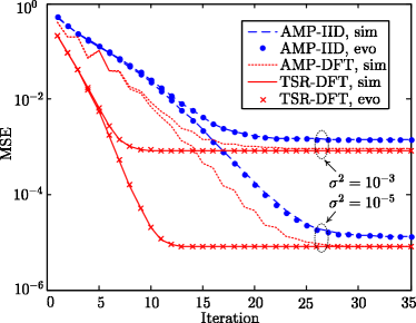
Figure 3: MSE performances of TSR and AMP. $\lambda=0.4$. $N=8192$. $M=5734\,(\approx 0.7N)$. The simulated MSEs are obtained by averaging over 500 realizations.

VI Conclusions

In this letter, we proved based on state evolution that TSR-DFT outperformed AMP-IID. In addition, our simulation results suggest that TSR-DFT converges faster than AMP-DFT. Possible future work includes extending the TSR algorithm to the IID setting and compare it with AMP-IID.

References

- [1] D. L. Donoho, A. Maleki, and A. Montanari, “Message-passing algorithms for compressed sensing,” in Proc. Nat. Acad. Sci., vol. 106, no. 45, Nov. 2009.
- [2] M. Bayati and A. Montanari, “The dynamics of message passing on dense graphs, with applications to compressed sensing,” IEEE Trans. Inf. Theory, vol. 57, no. 2, pp. 764–785, Feb. 2011.
- [3] S. Rangan. Generalized approximate message passing for estimation with random linear mixing. Preprint, 2010. [Online]. Available: http://arxiv.org/abs/1010.5141.
- [4] U. Kamilov, S. Rangan, A. Fletcher, and M. Unser, “Approximate message passing with consistent parameter estimation and applications to sparse learning,” IEEE Trans. Inf. Theory, vol. 60, no. 5, pp. 2969–2985, May, 2014.
- [5] F. Krzakala, M. Mézard, F. Sausset, Y. Sun, and L. Zdeborová, “Probabilistic reconstruction in compressed sensing: algorithms, phase diagrams, and threshold achieving matrices,” J. Statist. Mech.-Theory Exp., 2012.
- [6] D. Donoho, A. Javanmard, and A. Montanari, “Information-theoretically optimal compressed sensing via spatial coupling and approximate message passing,” in Proc. IEEE Int. Symp. Inf. Theory (ISIT), Jul. 2012, pp. 1231–1235.
- [7] J. Vila and P. Schniter, “Expectation-maximization gaussian-mixture approximate message passing,” IEEE Trans. Signal Process., vol. 61, no. 19, pp. 4658–4672, Oct. 2013.
- [8] J. Tan, Y. Ma, and D. Baron. Compressive imaging via approximate message passing with image denoising. Preprint, 2014. [Online]. Available: http://arxiv.org/abs/1405.4429.
- [9] C. Guo and M. E. Davies. Near optimal compressed sensing without priors: Parametric sure approximate message passing. Preprint, 2014. [Online]. Available: http://arxiv.org/abs/1409.0440.
- [10] G. Reeves and M. Gastpar, “The sampling rate-distortion tradeoff for sparsity pattern recovery in compressed sensing,” IEEE Trans. Inf. Theory, vol. 58, no. 5, pp. 3065–3092, May. 2012.
- [11] D. Guo and S. Verdu, “Randomly spread cdma: asymptotics via statistical physics,” IEEE Trans. Inf. Theory, vol. 51, no. 6, pp. 1983–2010, Jun. 2005.
- [12] D. Guo, D. Baron, and S. Shamai, “A single-letter characterization of optimal noisy compressed sensing,” in Proc. Allerton Conf. on Comm.,Control, and Computing, Sept. 2009, pp. 52–59.
- [13] A. Tulino, G. Caire, S. Verdu, and S. Shamai, “Support recovery with sparsely sampled free random matrices,” IEEE Trans. Inf. Theory, vol. 59, no. 7, pp. 4243–4271, Jul. 2013.
- [14] J. Barbier, F. Krzakala, and C. Schulke. Compressed sensing and approximate message passing with spatially-coupled fourier and hadamard matrices. Preprint, 2013. [Online]. Available: http://arxiv.org/abs/1312.1740.
- [15] S. Rangan, P. Schniter, and A. Fletcher, “On the convergence of approximate message passing with arbitrary matrices,” in Proc. IEEE Int. Symp. Inf. Theory (ISIT), Jun. 2014, pp. 236–240.
- [16] Y. Kabashima and M. Vehkapera, “Signal recovery using expectation consistent approximation for linear observations,” in Proc. IEEE Int. Symp. Inf. Theory (ISIT), Jun. 2014, pp. 226–230.
- [17] B. Cakmak, O. Winther, and B. Fleury, “S-amp: Approximate message passing for general matrix ensembles,” in Proc. ITW 2014, Nov. 2014, pp. 192–196.
- [18] J. Ma, X. Yuan, and L. Ping, “Turbo compressed sensing with partial dft sensing matrix,” IEEE Signal Process. Lett., vol. 22, no. 2, pp. 158–161, Feb. 2015.
- [19] C. Wen and K.Wong. Analysis of compressed sensing with spatially-coupled orthogonal matrices. Preprint, 2014. [Online]. Available: http://arxiv.org/abs/1402.3215.
- [20] M. Vehkapera, Y. Kabashima, and S. Chatterjee, “Analysis of regularized ls reconstruction and random matrix ensembles in compressed sensing,” in Proc. IEEE Int. Symp. Inf. Theory (ISIT), Jun. 2014, pp. 3185–3189.
- [21] C. Wen, J. Zhang, K. Wong, J. Chen, and C. Yuen. On sparse vector recovery performance in structurally orthogonal matrices via lasso. Preprint, 2014. [Online]. Available: http://arxiv.org/abs/1410.7295.
- [22] S. Oymak and B. Hassibi, “A case for orthogonal measurements in linear inverse problems,” in Proc. IEEE Int. Symp. Inf. Theory (ISIT), Jun. 2014, pp. 3175–3179.
- [23] C. Berrou and A. Glavieux, “Near optimum error correcting coding and decoding: turbo-codes,” IEEE Trans. Commun., vol. 44, no. 10, pp. 1261–1271, Oct. 1996.
- [24] S. M. Kay, Fundamentals of Statistical Signal Processing: Estimation Theory. NJ: Prentice-Hall PTR, 1993.
- [25] D. Guo, Y. Wu, S. Shamai, and S. Verdu, “Estimation in gaussian noise: Properties of the minimum mean-square error,” IEEE Trans. Inf. Theory, vol. 57, no. 4, pp. 2371–2385, Apr. 2011.