The inclusive jet production in the BFKL-Bartels approach with a running coupling introduced via bootstrap

Abstract

The inclusive cross-section for production of a jet with a given transverse momentum off a heavy nucleus is derived in the BFKL framework with a running coupling on the basis of the bootstrap relation. The cross-section depends on the same three different coupling constants as the total cross-section unlike the cross-section for gluon production derived in the dipole approach.

1 Introduction

Attempts to introduce the running coupling into the BFKL dynamics have a long history. As early as in 1986 L.N.Lipatov introduced the running coupling by using an approximate form of the BFKL equation and a semi-classical approach [1]. In his derivation a single running coupling $\alpha_{s}(r)$ appears with $r\to 0$. As a result he found that the cut in the complex angular momentum $J$ transforms into a sequence of poles, which condensate in a certain region depending on the total pomeron momentum. Later in our papers we introduced the running coupling into the BFKL equation by imposing the so-called bootstrap condition necessary for the fulfilment of unitarity  [2, 3]. In this approach three different running couplings appear. The structure of the singularities in the $J$ plane turned out dependent on the assumpsions about the uncontrolled low energy behaiour of the coupling. Remarkably it turned out that the bootstrap method correctly reproduced the running of the coupling in the reggeon interaction both in the forward and non-forward directions  [4, 5] explicitly calculated in  [6, 7, 8]. Still later, with the advent of the dipole picture and construction of the Balitski-Kovchegov equation for the pomeron in a heavy nucleus the running coupling was introduced by explicitly taking into account quark-antiquark loops in the evolution of the gluon density  [9, 10, 11, 12]. Again three different coupling constants appeared in the final equation. Remarkably this procedure turned out to be fully equivalent to the bootstrap approach, which leads to the same results with much less labour  [13]. Finally a few years ago the dipole approach was generalized to the case of inclusive production off a heavy nucleus  [14]. There at the leading order the number of different coupling constants proliferated up to seven. Still the authors made a conjecture for the form of the final inclusive cross-section, in whih the number of different coupling constants is reduced to three with one of them depending on the collinearity of the final jet components $\Lambda_{coll}$, that is essentially on the experimental setup.

In this paper we study the inclusive cross-section off a heavy nucleus within the bootstrap approach. It enables us to introduce the running coupling keeping the same number of them (three) as for the total cross-section. All the coupling constants remain depending only on the QCD scale $\Lambda$, with no dependence on the experimental conditions. Actually this approach allows to obtain only the inclusive cross-section for the production of a jet with a given transverse momentum, without specifying its other characteristics.

Note that this observable is different from the one calculated in  [14], where the jet (or a ”particle’) not only had a fixed transverse momentum but also had an upper bound on its collinearity $\Lambda_{coll}$. The latter was assumed to be small and only the singlular terms terms at $\Lambda_{coll}\to 0$ were kept. In the case of hadron production it appears that $\Lambda_{coll}$ would become the factorization scale between the hard process and fragmentation function. In our approach $\Lambda_{coll}$ seems to be effectively taken to infinity, making both the observable and its calculation very different.

In any case our cross-section has a well determined physical meaning and can well be related to experimental observations. So we believe that it is worth studying, especially since it turns out much simpler than the conjectured cross-sections in  [14], which are more specific and so dependent on the experimental resolution.

In our derivation we use the well-known two-dimensional transverse picture of BFKL and J.Bartels. (see e.g. [15]) We invoke the relative coefficients between different configurations in assumed correspondence with the standard AGK rules, which is confirmed by calculations with a fixed coupling.

2 Triple-Pomeron vertex

As mentioned in the Introduction, in this paper we follow the idea to introduce a running coupling via the bootstrap  [2, 3]. Derivation of the triple-pomeron vertex in the limit $N_{c}\to\infty$ then goes as presented in  [16, 17] for the fixed coupling case. The same derivation for the running coupling case is presented in  [13], which we briefly recapitulate here.

Basic formulas for the introduction of a running coupling via the bootstrap condition consist in expressing both the gluon trajectory $\omega$ and intergluon interaction in the vacuum channel $V$ in terms of a single function $\eta(q)$ of the gluon momentum, which then can be chosen to conform to the high-momentum behaviour of the gluon density with a running coupling. Explicitly

$$\omega(q)=-\frac{1}{2}N_{c}\int\frac{d^{2}q_{1}}{(2\pi)^{2}}\frac{\eta(q)}{\eta(q_{1})\eta(q_{2})},$$ (1)

$$V(q_{1},q_{2}|q^{\prime}_{1},q^{\prime}_{2})=N_{c}\Big{[}\Big{(}\frac{\eta(q_{1})}{\eta(q^{\prime}_{1})}+\frac{\eta(q_{2})}{\eta(q^{\prime}_{2})}\Big{)}\frac{1}{\eta(q_{1}-q^{\prime}_{1})}-\frac{\eta(q_{1}+q_{2})}{\eta(q^{\prime}_{1})\eta(q^{\prime}_{2})}\Big{]}.$$ (2)

In these definitions it is assumed that $q_{1}+q_{2}=q^{\prime}_{1}+q^{\prime}_{2}=q$. Note that the unsymmetric form (2) assumes that the initial pomeron with momenta $q^{\prime}_{1}$ and $q^{\prime}_{2}$ is ”amputated”, that is multiplied by $\eta(q^{\prime}_{1})\eta(q^{\prime}_{2})$. This factor appears explicitly in the denominators in (2). For arbitrary $\eta(q)$ the following bootstrap relation is satisfied:

$$\frac{1}{2}\int\frac{d^{2}q^{\prime}_{1}}{(2\pi)^{2}}V(q,q_{1},q^{\prime}_{1})=\omega(q)-\omega(q_{1})-\omega(q_{2}).$$ (3)

The fixed coupling corresponds to the choice

$$\eta^{fix}(q)=\frac{2\pi}{g^{2}}q^{2}.$$ (4)

Then one finds the standard expression for the trajectory $\omega(q)$ and

$$V^{fix}(q,q_{1},q^{\prime}_{1})=\frac{g^{2}N_{c}}{2\pi}V_{BFKL}(q,q_{1},q^{\prime}_{1}),$$

where $V_{BFKL}$ is the standard BFKL interaction. Note that the extra $2\pi$ in the denominator corresponds to the BFKL weight $1/(2\pi)^{3}$ in the momentum integration, which we prefer to take standardly as $1/(2\pi)^{2}$.

From the high-momentum behaviour of the gluon distribution with a running coupling one finds

$$\eta(q)=\frac{1}{2\pi}bq^{2}\ln\frac{q^{2}}{\Lambda^{2}},\ \ q^{2}>>\Lambda^{2},$$ (5)

where $\Lambda$ is the standard QCD parameter and

$$b=\frac{1}{12}\Big{(}11N_{c}-\frac{2}{3}N_{f}\Big{)}.$$ (6)

As to the behaviour of $\eta(q)$ at small momenta, we shall assume

$$\eta(0)=0,$$ (7)

which guarantees that the gluon trajectory $\omega(q)$ passes through zero at $q=0$ in accordance with the gluon properties. The asymptotic (5) and condition (7) are the only properties of $\eta(q)$ which follow from the theoretical reasoning. A concrete form of $\eta(q)$ interpolating between (7) and (5) may be chosen differently. One hopes that the following physical results will not strongly depend on the choice.

Our old derivation in  [16] of the triple-pomeron vertex was actually based on the property (7) obviously valid for (4), the bootstrap relation and the relation between the Bartels transition vertex for a fixed coupling constant $W^{fix}_{2\to 3}$ and intergluon BFKL interaction $V_{BFKL}$ (Eq. (12) in  [16])

$$W^{fix}_{2\to 3}(1,2,3|1^{\prime},3^{\prime})=V_{BFKL}(2,3|1^{\prime}-1,3^{\prime})-V_{BFKL}(12,3|1^{\prime}3^{\prime}).$$ (8)

Here and in the following we frequently denote gluon momenta just by numbers: $1\equiv q_{1}$, $1^{\prime}\equiv q^{\prime}_{1}$ etc. Also we use $12\equiv q_{1}+q_{2}$. All the rest conclusions were obtained from these three relations in a purely algebraic manner.

If we define the transition vertex for a running coupling by a similar relation in terms of the new intergluon vertex $V$, Eq. (2),

$$W_{2\to 3}(1,2,3|1^{\prime},3^{\prime})=V(2,3|1^{\prime}-1,3^{\prime})-V(12,3|1^{\prime}3^{\prime}).$$ (9)

where $V$ is given by (2) then all the results will remain valid also for arbitrary $\eta(q)$ satisfying (7) and thus for a running coupling, provided $\eta(q)$ is chosen appropriately. In this way in the momentum space one can find the the three-pomeron vertex with the running coupling  [13] and write the corresponding Balitski- Kovchegov equation . It has a simpler form in the cordinate space. In the forward case at fixed impact parameter $b$ the resulting Balitski-Kovchegov equation with the running coupling  [13] is obtained as

$$\frac{\partial}{\partial y}\Phi(y,r)=\frac{1}{2\pi^{2}}N_{c}\int d^{2}r_{2}d^{2}r_{3}\delta(r-r_{1}+r_{2})\Big{(}\frac{\alpha_{s}(r_{1})}{r_{1}^{2}}+\frac{\alpha_{s}(r_{2})}{r_{2}^{2}}-2\frac{\alpha_{s}(r_{1})\alpha_{s}(r_{2})}{\alpha_{s}(r_{1},r_{2})}\frac{{\bf r}_{1}{\bf r}_{2}}{r_{1}^{2}r_{2}^{2}}\Big{)}$$

$$\Big{(}\Phi(y,r_{1},b)+\Phi(y,r_{2},b)-\Phi(y,r,b)-\Phi(y,r_{1},b)\Phi(y,r_{2},b)\Big{)}.$$ (10)

where the two running coupling constants $\alpha_{s}(r)$ and $\alpha_{s}(r_{1},r_{2})$ are defined as

$$\alpha_{s}(r)=-\pi^{2}r^{2}f(r,r),\ \ \alpha_{s}(r_{1},r_{2})=-\pi^{2}({\bf r}_{1}{\bf r}_{2})\frac{f(r_{1},r_{1})f(r_{2},r_{2})}{f(r_{1},r_{2})}$$ (11)

and

$$f(r_{1},r_{2})=\int d^{2}\rho\tilde{\eta}(\rho)\xi(r_{1}-\rho)\xi(r_{2}-\rho).$$ (12)

where $\tilde{\eta}(r)$ is the Fourier transform of $\eta(q)$ and $\xi(r)$ is the Fourier transform of $1/\eta(q)$. Eq. (10) formally coincides with the running coupling equation obtained in the dipole aproach in  [9, 11]. However in our approach the couplings $\alpha_{s}(r)$ and $\alpha_{s}(r_{1},r_{2})$ are not directly taken from the QCD. Rather it is function $\eta(q)$ that is taken from the QCD and the coupling constants are determined by it.

3 Inclusive cross-sections

Diagrammatically contributions to the forward amplitude for the collision of the projectile with the nucleus are identical to those which appear in the fixed coupling case. The difference is totally restricted to the new form of the reggeized gluon trajectory, interaction between the reggeons and the splitting vertex. Correspondingly the inclusive cross-sections will be obtained either by cutting the interaction in the uppermost pomeron (before all splitting) or by cutting the first splitting vertex. All the rest contributions will be eliminated by the AGK cancellations.

However one should take into account that the inclusive cross-sections obtained in this manner do not refer to precisely gluon production. The form of the function $\eta(p)$ desribing the intermediate $s$-channel state with the single-loop $\beta$ function includued implies that one has to take into account not only the single real gluon state but also states which contribute to this $\beta$-function, namely the quark-antiquark and two-gluon states. So the inclusive cross-section obtained by fixing the intermediate $s$-state momentum $p$ actually refers to all possible states having this momentum. It does not discriminate between contributions from gluons (single or in pairs) and (anti)quarks. So it is rather the inclusive cross-section for emission of a jet with a total transverse momentum $p$. The diagrams for this cross-section are illustrated in Fig. 1. We think that this quantity has a well-defined physical meaning and is accessible for experimental observation and so worth theoretical investigation. In all the following we study precisiely this generalized inclusive cross-section for jet production.

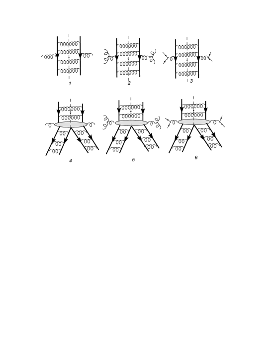
Figure 1: Diagrams for the cross-section corresponding to emission from the upper pomeron (1-3) and from the triple pomeron vertex (4-6). Thick solid lines denote reggeons, thin lines denote real quarks, wavy lines denote real and virtual gluons.

4 Jet production from the pomeron

This part of the total cross-section is calculated in full analogy with the fixed coupling case. If only a single pomeron is exchanged between the projectile and target then we have the impulse approximation contribution

$$I(Y,y,p)=\frac{(2\pi)^{3}d\sigma}{dyd^{2}p}=\frac{4N_{c}}{\eta(p)}\int\frac{d^{2}k}{(2\pi)^{2}}\eta(k)\eta(p-k)P(Y-y,p-k)P(y,k).$$ (13)

Here it is assumed that the ”semi-amputated” forward pomeron wave function $\phi(y,p)=\eta(p)P(y,p)$ in the momentum space satisfies the equation

$$\frac{\partial\phi(y,p)}{\partial y}=2\omega(p)\phi(y,p)+2N_{c}\int\frac{d^{2}k}{(2\pi)^{2}}\frac{P(y,k)}{\eta(p-k)}\phi(y,k).$$ (14)

With a fixed coupling $P(y,p)$ obviously has order $g^{4}$ so that $I$ has order $g^{6}$, which takes into account two impact factors each of order $g^{2}$

For a nucleus target the pomeron coupled to the target has to be substituted by the solution of the Balitski-Kovchegov equation (10) at fixed impact parameter $b$ (transformed to the momentum space):

$$I_{1}(Y,y,p,b)=\frac{(2\pi)^{3}d\sigma_{1}}{dyd^{2}pd^{2}b}=\frac{4N_{c}}{\eta(p)}\int\frac{d^{2}k}{(2\pi)^{2}}\eta(k)\eta(p-k)P(Y-y,p-k)\Phi(y,k,b).$$ (15)

5 Jet production from the vertex: generalities

The three-pomeron vertex has a fixed rapidity and does not include evolution. This makes it possible to study the contribution to jet emission from the vertex in the lowest order of perturbation theory, that is for the target consisting of only two centers. It also allows to simplify treatment choosing for the projectile and target quarks, modeling the pomeron exchanges by colorless double reggeon exchanges. The inclusive cross-section will be obtained from the diagrams for the forward scattering off two centers, in which reggeon interactions and splittings are described by functions $V$ and $W$, given by Eqs. (2) and (9) with the running coupling. All the diagrams may be divided into two configurations depending on the way the four final reggeons are combined into pomerons. The diffractive one includes diagrams with two consecutive colourless exchanges (Figs. 2-4). The non-diffractive configuration includes diagrams with parallel colourless exchanges (Figs. 5-7) when one of the colourless pair of reggeons is enclosed in the other. In these diagrams vertical lines denote reggeons, solid horizontal lines denote projectile and target quarks and wavy lines denote $s$-channel gluons. Diagrams in which the colourless pairs partially overlap do not give contribution to the inclusive cross-section and we do not show them. Note that the number of reggeons coupled to the projectile may vary from two to four. However, as shown long ago, all contributions reduce to that of a colourless pair of reggeons forming the initial pomeron (amputated with the forms (2) and (9)). If one subtracts the contribution from the so-called reggeized term (see e.g.  [15]) or alternatively from the Glauber initial condition in the dipole formalism) the the rest gives the contribution from the triple pomeron vertex, which is our goal

To obtain the inclusive cross-section for the production of a jet with momentum $p$ one has to fix function $\eta(p)$ in intermediate states in the $s$ channel. These intermediate states are obtained by cutting the diagrams in the $s$-channel. Different cuts may pass through one of the targets (single cuts, S), through both targets (double cuts, DC) or do not pass through targets at all (diffractive cuts, D). In the diffractive configuration only diffractive and single cuts are possible. In the non-diffractive configuration only single and double cuts are possible. According to the AGK rules the relative weights of the contributions from diffractive, single and double cuts are $1:-1:2$.

We denote the reggeon momenta of the first final pomeron as $q_{1}$ and $q_{2}$ and of the second as $q_{3}$ and $q_{4}$. In the forward direction $q_{2}=-q_{1}$ and $q_{3}=-q_{4}$. So the final pomerons carry momenta $q_{1}$ and $q_{4}$.

6 A. Diffractive configuration

We divide all contributions according to the number of initial reggeons (R): A2, A3 and A4 for two three and four initial reggeons respectively.

6.1 A4: 4R$\to$ 4R

We have 6 diagrams shown in Fig. 2.

Figure 2: 4R$\to$ 4R in the diffractive configuration

They contribute either in D or S configurations. Due to assumed relation between D and S diagrams 2 and 5 are ancelled. 1 and 6 give only S. 4 contains only D. Finally 3 contains D+2S=-D. Due to the properies of the pomeron $SD_{1}=SD_{6}=0$. So we are left only with 3 and 4. Colour factors:

$$C_{3}=C_{4}=\frac{1}{4}N_{c}^{4}.$$

So taking $(-V)$ for the interaction we find

$$(3)=-C_{3}(-V(q_{1},q_{4}|q_{1}+p,q_{4}-p)),$$ (16)

$$(4)=C_{4}(-V(-q_{1},-q_{4}|-q_{1}+p,-q_{4}+p)).$$ (17)

Changing signs of $q_{1}$ and $q_{4}$ does not change $V$. So in the end (3)+(4)=0 and the diagrams $D_{4\to 4}$ give no contribution.

6.2 A2: 2R$\to$ 4R

There is a single diagram 2R$\to$4R, shown in Fig. 3.

Figure 3: 2R$\to$ 4R in the diffractive configuration

It contributes in both D and S configurations. Colour factor is $C=N_{c}^{4}$. The D contribution is

$$A_{2D}=-CW(q_{1},-q_{1}-q_{4},q_{4}|p,-p).$$ (18)

The two S contributions give

$$A_{2SD}=+CW(q_{1},-q_{1}-q_{4},q_{4}|q_{1}+p,-q_{1}-p)+CW(q_{1},-q_{1}-q_{4},q_{4}|-q_{4}+p,q_{4}-p).$$ (19)

6.3 A3: 3R$\to$ 4R

We have 4 diagrams which contribute in $D$ or $SD$ configurations, shown in Fig. 4

Figure 4: 3R$\to$4R in the diffractive configuration

Note that $C_{1}=C_{2}=-1/2$ and $C_{3}=C_{4}=+1/2$.

So the S contribution from (1) cancels the left S contribution from (3) and the S conttibution from 2 cancels the right contribution from (4). Moreover the D contribution from (3) cancels the right SD contribution from (3) and the D contribution from (4) canceles the left S contribution drom (4). As a result the only remaining contribution is D contribution from diagrams (1) and (2)

$$A3=A3_{D}=-C_{1}W(q_{1},-q_{1},-q_{4}|p,-q_{4}-p)-C_{1}W(-q_{1},-q_{4},q_{4}|-q_{1}+p,-p),$$ (20)

where we have taken into account that D contributions from (1) and (2) are equal.

6.4 The total diffractive contribution

Suppressing the overall colour coefficient $N_{c}^{4}$ we have found

$$A=A_{2D}+A_{2S}+A_{3D}=-W(q_{1},-q_{1}-q_{4},q_{4}|p,-p)$$

$$+W(q_{1},-q_{1}-q_{4},q_{4}|q_{1}+p,-q_{1}-p)+W(q_{1},-q_{1}-q_{4},q_{4}|-q_{4}+p,q_{4}-p)$$

$$-\frac{1}{2}W(q_{1},-q_{1},-q_{4}|p,-q_{4}-p)-\frac{1}{2}W(-q_{1},-q_{4},q_{4}|-q_{1}+p,-p).$$

7 B. Non-diffractive configuration

7.1 B4: 4R$\to$ 4R

Six diagrams with transitions 4R$\to$ 4R are shown in Fig. 5.

Figure 5: 4R$\to$ 4R in the non-diffractive configuration

Since the double cut (DC) contribuition enters with coefficient 2 diagram (3) is cancelled. Diagrams 2 and 5 give the same contribution. The S in both cancels one half of the DC contribution, so that the total coefficient is reduced to 1. Diagram (4) is zero. Diagram 1 and 6 contribute only to the S contribution. So in the end the DC and S contributions are

$$B4_{DC}=(2)+(5),\ \ B4_{S}=-(1)-(6).$$ (21)

Colour factors are

$$C_{2}=C_{5}=-\frac{1}{4}N_{c}^{4},\ \ C_{1}=c_{6}=\frac{1}{4}N_{c}^{4}.$$

So we get (again suppressing $N_{c}^{4}$)

$$B4_{DC}=\frac{1}{4}\Big{(}V(-q_{4},-q_{1}|-q_{4}+p,-q_{1}-p),\ \ +V(q_{1},q_{4}|q_{1}+p,q_{4}-p)\Big{)},$$ (22)

$$B4_{S}=\frac{1}{4}\Big{(}V(-q_{4},q_{1}|-q_{4}+p,q_{1}-p)+V(-q_{1},q_{4}|-q_{1}+p,q_{4}-p)\Big{)}.$$ (23)

7.2 B2: 2R$\to$ 4R

There is a single diagram for transitions 2$\to 4$ shown in Fig. 6.

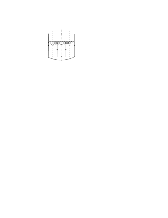
Figure 6: 2R$\to$ 4R in the non-diffractive configuration

It contains DC and S contributions. The colour factor is $C=N^{4}$, so suppressing it

$$B2_{DC}=-2W(-q_{4},0,q_{4}|q_{1}-q_{4}+p,-q_{1}+q_{4}-p)$$ (24)

and

$$B2_{S}=2W(-q_{4},0,q_{4}|-q_{4}+p,q_{4}-p).$$ (25)

In fact the S contribution gives zero: it does not depend on $q_{1}$.

7.3 B3: 3R$\to$ 4R

Four diagrams with transitions 3$\to$4 are shown in Fig. 7.

Figure 7: 3R$\to$ 4R in the non-diffractive configuration

We observe that the right S contribution in (3) cancels one half of the DC contribution in (3) and the left S contribution in (4) cancels one half of the DC contribution in (3). Thus we get

$$B3_{DC}=2(1)_{DC}+2(2)_{DC}+(3)_{DC}+(4)_{DC}$$ (26)

and

$$B3_{S}=-(1)_{S}-(2)_{S}-(3)_{Sl}-(4)_{Sr},$$ (27)

where $Sl$ and $Sr$ refer to left and right single cuts.

The colour factors are

$$C_{1}=C_{2}=\frac{1}{2}N_{c}^{4},\ \ C_{3}=C_{4}=-\frac{1}{4}N_{c}^{4}.$$

So suppressing $N_{c}^{4}$

$$B3_{DC}=-W(-q_{4},q_{1},-q_{1}|-q_{4}+q_{1}+p,-q_{1}-p)+-W(q_{1},-q_{1},q_{4}|q_{1}+p,q_{4}-q_{1}-p)$$

$$++\frac{1}{4}W(-q_{4},q_{1},q_{4}|q_{1}-q_{4}+p,q_{4}-p)+\frac{1}{4}W(-q_{4},-q_{1},q_{4}|-q_{4}+p,q_{4}-q_{1}-p)$$

and

$$B3_{S}=\frac{1}{2}W(-q_{4},q_{1},-q_{1}|-q_{4}+p,-p)\frac{1}{2}W(q_{1},-q_{1},q_{4}|p,q_{4}-p)$$

$$-\frac{1}{4}W(-q_{4},q_{1},q_{4}|-q_{4}+p,q_{1}+q_{4}-p)-\frac{1}{4}W(-q_{4},-q_{1},q_{4}|-q_{1}-q_{4}+p,q_{4}-p).$$

7.4 The total non-diffractive contribution

$$B=B4_{DC}+B4_{SDC}+B2_{DC}+B2_{S}+B3_{DC}+B3_{S}=$$

$$\frac{1}{4}\Big{(}V(-q_{4},-q_{1}|-q_{4}+p,-q_{1}-p)+V(q_{1},q_{4}|q_{1}+p,q_{4}-p)$$

$$+(V(-q_{4},q_{1}|-q_{4}+p,q_{1}-p)+V(-q_{1},q_{4}|-q_{1}+p,q_{4}-p)\Big{)}$$

$$-2W(-q_{4},0,q_{4}|q_{1}-q_{4}+p,-q_{1}+q_{4}-p)$$

$$-W(-q_{4},q_{1},-q_{1}|-q_{4}+q_{1}+p,-q_{1}-p)-W(q_{1},-q_{1},q_{4}|q_{1}+p,q_{4}-q_{1}-p)$$

$$+\frac{1}{4}W(-q_{4},q_{1},q_{4}|q_{1}-q_{4}+p,q_{4}-p)+\frac{1}{4}W(-q_{4},-q_{1},q_{4}|-q_{4}+p,q_{4}-q_{1}-p)$$

$$+\frac{1}{2}W(-q_{4},q_{1},-q_{1}|-q_{4}+p,-p)+\frac{1}{2}W(q_{1},-q_{1},q_{4}|p,q_{4}-p)$$

$$-\frac{1}{4}W(-q_{4},q_{1},q_{4}|-q_{4}+p,q_{1}+q_{4}-p)-\frac{1}{4}W(-q_{4},-q_{1},q_{4}|-q_{1}-q_{4}+p,q_{4}-p).$$

8 Jet production from the vertex: the final form

The found contributions to inclusive cross-sections from the two configurations are numerous and contain many terms. To analyze them it is convenient to introduce function

$$F(q|p)\equiv(q|p)=\frac{\eta(q)}{\eta(p)\eta(q-p)}=(q|q-p)=(-q|-p).$$ (28)

In terms of this function

$$V(q_{1},q_{2}|k_{1},k_{2})=(k_{12}|k_{1})-(q_{1}|k_{1})-(q_{2}|k_{2}),$$ (29)

$$W(q_{1},q_{2},q_{3}|k_{1},k_{2})=(k_{12}|k_{1})-(q_{12}|k_{1})-(q_{23}|k_{2})+(q_{2}|k_{1}-q_{1}),$$ (30)

where $k_{12}=k_{1}+k_{2}$ etc. The analysis of the found inclusive cross-section in terms of function $F(q|p)$ is performed in Appendix. It is important to take into account that all contributions which do not depend on the momenta of one of the final pomerons, $q_{1}$ or $q_{4}$, vanish, since the Pomeron vanishes when its two reggeized gluons are at the same spatial point.

After some cancellations one finally finds the contribution

$$A+B=2\Big{[}(q_{14}|p)+(q_{14}|-p)\Big{]}.$$ (31)

With the fixed coupling constant one finds instead

$$(A+B)^{fix}=\frac{g^{2}}{\pi}\Big{[}\frac{q_{14}^{2}}{p^{2}(q_{14}-p)^{2}}+\Big{(}p\to-p\Big{)}\Big{]}.$$ (32)

It was shown that in the fixed coupling case half of this expression comes from the reggeized piece (or the Glauber initial condition in the dipole approach)  [19]. By the same reasoning the contribution from the triple pomeron vertex is one half of (31). As we see, to find our inclusive cross-section for jet production with the running couling all the necessary change is the substitution of all momenta according to the rule

$$q^{2}\to\frac{g^{2}}{2\pi}\eta(q).$$ (33)

Using the known form of the inclusive cross-section in the fixed coupling case ([18], see also [19] for closer notations) one can immediately write the final expression for it with the running coupling as

$$I_{2}(Y,y,p)=-\frac{2N_{c}}{\eta(p)}\int\frac{d^{2}q_{1}d_{2}q_{4}}{(2\pi)^{4}}\eta(q_{14}-p)P(Y-y,q_{14}-p)\eta(q_{14})\Phi(y,q_{1})\Phi(y,q_{4}).$$ (34)

The total inclusive cross-section is the sum of (15) and (34):

$$I(Y,y,p,b)=\frac{(2\pi)^{3}d\sigma}{dyd^{2}pd^{2}b}=\frac{2N_{c}}{\eta(p)}\int\frac{d^{2}q_{1}d^{2}q_{4}}{(2\pi)^{4}}$$

$$\eta(q_{(}14-p)P(Y-y,q_{14}-p)\Big{[}2\eta(q_{1})\Phi(y,q_{1},b))(2\pi)^{2}\delta(q_{4})-\eta(q_{14})\Phi(y,q_{1})\Phi(y,q_{4})\Big{]}.$$ (35)

9 Discussion

Our final expression for the inclusive cross-section Eq. (35) has a strong similarity with the one conjectured in  [14]). It contains three factors $\eta$, which can be put in correspondence with the three coupling constants depending on different arguments in  [14]. However in our formula the arguments of functions $\eta$ directly depend on the three momenta involved: that of the observed jet and two of the gluon distributions involved. In contrast, in the conjecture of  [14] the argument of one of the coupling constants depends only on the assumed value of collinearity of the observed jet and the arguments of two others are complex and depend on all three momenta in a very complicated manner. However, as mentioned in the Introduction, the literal comparison of the two cross-sections is not possible, since in fact they refer to different processes: to jet production with a given momentum in our case and with additional restriction on jet collinearity in  [14]. Besides the cross-section in  [14] is after all only conjecture, whereas ours is more or less consitently derived from the bootstrap condition which demonstrated its validity for the total cross-section.

It remains to be seen by practical applications to what extent this difference is felt in the actual inclusive cross-sections. To do this consistently one has to previously solve our equation for the unintegrated gluon density (10). With all its similarity to the currently used equation in the dipole picture, the actual values of the three running couplings involved are not identical, so that the already found solutions in the dipole picture cannot be directly used for our inclusive cross-section. We postpone this problem for future studies.

In conclusion we stress that that our equations take in account terms of the order $(\alpha(q))^{n}$ with $\alpha(q)$ taken in the leading order. Subleading terms of the relative order $1/\ln(q^{2}/\Lambda^{2})$ remain undetermined, since they correspond to the next-to-leading order in the running coupling.

10 Appendix.Analysis of the found inclusive cross-sections

In terms of $F$ we find

$$A=-\Big{(}0-(-q_{4}|p)-(-q_{1}|-p)+(-q_{1}-q_{4}|p-q_{1})\Big{)}$$

$$+\Big{(}0-(-q_{4}|q_{1}+p)-(-q_{1}|-q_{1}-p)+(-q_{1}-q_{4}|p)\Big{)}$$

$$+\Big{(}0-(-q_{4}|-q_{4}+p)-(-q_{1}|q_{4}-p)+(-q_{1}-q_{4}|-p)\Big{)}$$

$$\frac{1}{2}\Big{(}(-q_{4}|p)-(-q_{1}-q_{4}|-q_{4}-p)+(-q_{1}|p-q_{1})\Big{)}\frac{1}{2}\Big{(}(-q_{1}|-p)-(-q_{1}-q_{4}|-q_{1}+p)+(-q_{4}|p)\Big{)}$$

We take into account that terms which do not depend on $q_{1}$ or do not depend on $q_{4}$ are integrated ober $q_{1}$ and $q_{4}$ to give zero. Dropping these terms

$$A=-(-q_{1}-q_{4}|p-q_{1})-(-q_{4}|q_{1}+p)+(-q_{1}-q_{4}|p)$$

$$-(-q_{1}|q_{4}-p)+(-q_{1}-q_{4}|-p)$$

$$-\frac{1}{2}(-q_{1}-q_{4}|-q_{4}-p)-\frac{1}{2}(-q_{1}-q_{4}|-q_{1}+p)$$

Now non-diffractive contributions

$$B=\frac{1}{4}\Big{(}(-q_{4}-q_{1}|-q_{4}+p)-(-q_{4}|-q_{4}+p)-(-q_{1}|-q_{1}-p)$$

$$+(q_{1}+q_{4}|q_{1}+p)-(q_{1}|q_{1}+p)-(q_{4}|q_{4}-p)$$

$$+(q_{1}-q_{4}|-q_{4}+p)-(-q_{4}|-q_{4}+p)-(q_{1}|q_{1}-p)$$

$$+(q_{4}-q_{1}|-q_{1}+p)(-q_{1}|-q_{1}+p)-(q_{4}|q_{4}-p)\Big{)}$$

$$-2\Big{(}-(-q_{4}|q_{1}-q_{4}+p)-(q_{4}|-q_{1}+q_{4}-p)\Big{)}$$

$$-\Big{(}(-q_{4}|-q_{1}-p)-(q_{1}-q_{4}|q_{1}-q_{4}+p)+(q_{1}|q_{1}+p)\Big{)}$$

$$-\Big{(}(q_{4}|q_{1}+p)-(q_{4}-q_{1}|q_{4}-q_{1}-p)+(-q_{1}|p)\Big{)}$$

$$+\frac{1}{4}\Big{(}(q_{1}|q_{4}-p)-(q_{1}-q_{4}|q_{1}-q_{4}+p)-(q_{1}+q_{4}|q_{4}-p)+(q_{1}|q_{1}+p)\Big{)}$$

$$+\frac{1}{4}\Big{(}(-q_{1}|-q_{4}+p)-(-q_{1}-q_{4}|-q_{4}+p)-(q_{4}-q_{1}|q_{4}-q_{1}-p)+(-q_{1}|p)\Big{)}$$

$$+\frac{1}{2}\Big{(}(-q_{4}|-p)-(q_{1}-q_{4}|-q_{4}+p)+(q_{1}|-p)\Big{)}+\frac{1}{2}\Big{(}(q_{4}|p)-(q_{4}-q_{1}|q_{4}-p)+(-q_{1}|-p)\Big{)}$$

$$-\frac{1}{4}\Big{(}(q_{1}|-q_{4}+p)-(q_{1}-q_{4}|-q_{4}+p)-(q_{1}+q_{4}|q_{1}+q_{4}-p)(q_{1}|p)\Big{)}$$

$$-\frac{1}{4}\Big{(}(-q_{1}|q_{4}-p)-(-q_{1}-q_{4}|-q_{1}-q_{4}+p)-(q_{4}-q_{1}|q_{4}-p)+(-q_{1}|-p)\Big{)}$$

Again we remove terms which do not depend on one of the variables $q_{1}$ or $q_{4}$. Dropping these terms

$$B=\frac{1}{4}\Big{(}(-q_{4}-q_{1}|-q_{4}+p)+(q_{1}+q_{4}|q_{1}+p)+(q_{1}-q_{4}|-q_{4}+p)+(q_{4}-q_{1}|-q_{1}+p)\Big{)}$$

$$-2\Big{(}-(-q_{4}|q_{1}-q_{4}+p)-(q_{4}|-q_{1}+q_{4}-p)\Big{)}$$

$$-\Big{(}(-q_{4}|-q_{1}-p)-(q_{1}-q_{4}|q_{1}-q_{4}+p)\Big{)}-\Big{(}-(q_{4}-q_{1}|q_{4}-q_{1}-p)+(q_{4}|q_{1}+p)\Big{)}$$

$$+\frac{1}{4}\Big{(}(q_{1}|q_{4}-p)-(q_{1}-q_{4}|q_{1}-q_{4}+p)-(q_{1}+q_{4}|q_{4}-p)\Big{)}$$

$$+\frac{1}{4}\Big{(}(-q_{1}|-q_{4}+p)-(-q_{1}-q_{4}|-q_{4}+p)-(q_{4}-q_{1}|q_{4}-q_{1}-p)\Big{)}$$

$$+\frac{1}{2}\Big{(}-(q_{1}-q_{4}|-q_{4}+p)\Big{)}+\frac{1}{2}\Big{(}-(q_{4}-q_{1}|q_{4}-p)\Big{)}$$

$$-\frac{1}{4}\Big{(}(q_{1}|-q_{4}+p)-(q_{1}-q_{4}|-q_{4}+p)-(q_{1}+q_{4}|q_{1}+q_{4}-p)\Big{)}$$

$$-\frac{1}{4}\Big{(}(-q_{1}|q_{4}-p)-(-q_{1}-q_{4}|-q_{1}-q_{4}+p)-(q_{4}-q_{1}|q_{4}-p)\Big{)}$$

Next we simplify our expressions using the possibility to change $q_{1,4}\leftrightarrow-q_{1,4}$ and $q_{1,4}\leftrightarrow q_{4,1}$. We reduce all terms to two basic structures $(q_{14}|a)$ and $(q_{1}|a)$. Then we get

$$A=-(q_{14}|q_{1}+p)-(q_{1}|q_{4}+p)+(q_{14}|p)-(q_{1}|q_{4}-p)+(q_{14}|-p)$$

$$-\frac{1}{2}(q_{14}|q_{1}+p)-\frac{1}{2}(q_{14}|q_{1}+p)$$

and

$$B=(q_{14}|q_{1}+p)-2\Big{(}-(q_{1}|q_{4}-p)-(q_{1}|q_{4}+p)\Big{)}$$

$$-(q_{1}|q_{4}-p)+(q_{14}|-p)+(q_{14}|p)-(q_{1}|q_{4}+p)$$

$$+\frac{1}{4}\Big{(}(q_{1}|q_{4}-p)-(q_{14}|-p)-(q_{14}|q_{1}+p)\Big{)}$$

$$+\frac{1}{4}\Big{(}(q_{1}|q_{4}+p)-(q_{14}|q_{1}+p)-(q_{14}|p)\Big{)}-(q_{14}|q_{1}+p)$$

$$-\frac{1}{4}\Big{(}(q_{1}|q_{4}+p)-(q_{14}|q_{1}+p)-(q_{14}|p)\Big{)}$$

$$-\frac{1}{4}\Big{(}(q_{1}|q_{4}-p)-(q_{14}|-p)-(q_{14}|q_{1}+p)\Big{)}$$

Note that

$$(q_{14}|q_{1}-p)=(q_{14}|q_{4}-p)=(q_{14}|q_{1}+p)$$

Let us find the coefficients for our basic structures

$$(q_{14}|q_{1}+p)$$

A2:-1, A3:+1, B4:+1,B2: 0,B3:-1/4-1/4-1+1/4+1/4=-1, total=0.

$$(q_{1}|q_{4}-p)$$

A2:-1, A3:0, B4:0, B2:2, B3:-1+1/4-1/4=-1, total=0.

$$(q_{1}|q_{4}+p)$$

A2:-1, A3:0, B4:0, B2:+2, B3:-1+1/4-1/4=-1, total=0.

$$(q_{14}|p)$$

A2:+1, A3:0, B4:0, B2:0, B3:+1-1/4+1/4=+1, total =2.

$$(q_{14}|-p)$$

A2:+1, A3:0, B4:0, B2:0, B3:+1-1/4+1/4=1, total =2.

This brings us to the final result (31).

11 Acknowledgements

The author would like to thank Yu. Kovchegov for numerous informative discussions. This work has been supported by grants RFFI 11.15.360.2015 and SPSU 11,38.223.2015.

References

• [1] Zh.Eksp.Teor.Fiz 90 (1986) 1536 (Sov.Phys. JETP 63 (1986) 904).
• [2] M.A.Braun, Phys.Lett. B 345 (1995) 155.
• [3] M.A.Braun, Phys.Lett. B 348 (1995) 190.
• [4] M.A.Braun, G.P.Vacca, Phys. Lett. B 454 (1999) 319
• [5] M.A.Braun, G.P.Vacca, Phys. Lett. B 477 (2000) 156
• [6] V.S.Fadin, L.N.Lipatov, Phys. Lett. B 429(1998) 127
• [7] G.Camici, M.Ciafaloni, Phys. Lett. B 395 (1997) 118.
• [8] V.S.Fadin, R.Fiore, A.Papa, Phys. Rev. D 60 (1999) 074025.
• [9] Yu.V.Kovchegov and H.Weigert, hep-ph/0609090.
• [10] E.Gardi, J.Kuokkanen, K.Rummukainen, H.Weigert, Nucl. Phys. A 784 (2007) 282
• [11] Yu.V.Kovchegov and H.Weigert, hep-ph/0612071.
• [12] I.I.Balitsky, Phys. Rev. D 75 (2007) 014001
• [13] M.A.Braun, Eur. Phys. J. C 51 (2007) 625.
• [14] W.A.Horowitz and Yu.V.Kovchegov, Nucl. Phys. A 849 (2011) 72.
• [15] J.Bartels and C.Ewerz, JHEP 9909 (1999) 026
• [16] M.A.Braun, Eur. Phys. J C 6 (1999) 321.
• [17] M.A.Braun and G.P.Vacca, Eur. Phys. J. C 6 (1999) 147.
• [18] Yu.V.Kovchegov and K.Tuchin, Phys. Rev. D 65 (2002) 074026.
• [19] M.A.Braun, Eur. Phys. J C 48 (2006) 501. (1999) 319; B 447 (2000) 156. 074025. (1999) 114036.