Discrete Signal Reconstruction by
Sum of Absolute Values

Abstract

In this letter, we consider a problem of reconstructing an unknown discrete signal taking values in a finite alphabet from incomplete linear measurements. The difficulty of this problem is that the computational complexity of the reconstruction is exponential as it is. To overcome this difficulty, we extend the idea of compressed sensing, and propose to solve the problem by minimizing the sum of weighted absolute values. We assume that the probability distribution defined on an alphabet is known, and formulate the reconstruction problem as linear programming. Examples are shown to illustrate that the proposed method is effective.

I Introduction

Signal reconstruction is a fundamental problem in signal processing. Recently, a paradigm called compressed sensing [1, 2, 3] has been proposed for signal reconstruction from incomplete measurements. The idea of compressed sensing is to utilize the property of sparsity in the original signal; if the original signal is sufficiently sparse, practical algorithms such as the basis pursuit [4], the orthogonal matching pursuit [5], etc, may give exact recovery under an assumption on the measurement matrix (see e.g. [3]).

On the other hand, it is also important to reconstruct discrete signals whose elements are generated from a finite alphabet with a known probability distribution. This type of reconstruction, called discrete signal reconstruction, arises in black-and-white or grayscale sparse image reconstruction [6, 7], blind estimation in digital communications [8], machine-type multi-user communications [9], discrete control signal design [10], to name a few.

The difficulty of discrete signal reconstruction is that the reconstruction has a combinatorial nature and the computational time becomes exponential. For example, 200-dimensional signal reconstruction with two symbols (i.e. binary signal reconstruction) needs at worst about $1.5\times 10^{36}$ years with a computer of 34 peta FLOPS (see Section II below), which cannot be executed, obviously.

To overcome this difficulty, we borrow the idea of compressed sensing based on $\ell^{1}$ optimization as used in the basis pursuit [4]. Our idea is that if the original discrete signal, say ${\boldsymbol{x}}$, includes $L$ symbols $r_{1},r_{2},\dots,r_{L}$, then each vector ${\boldsymbol{x}}-r_{i}$ is sparse. For example, a binary vector ${\boldsymbol{x}}$ on alphabet $\{1,-1\}$ includes a number of $1$ and $-1$, and hence both ${\boldsymbol{x}}-1$ and ${\boldsymbol{x}}+1$ are sparse. To recover such a discrete signal, we propose to minimize the sum of weighted absolute values of the elements in ${\boldsymbol{x}}-r_{i}$. The weights are determined by the probability distribution on the alphabet. The problem is reduced to a standard linear programming problem, and effectively solved by numerical softwares such as cvx in MATLAB [11, 12].

For discrete signal reconstruction, there have been researches based on compressed sensing, called integer compressed sensing: [13] has proposed a Bayesian-based method, which works only for binary sparse signals (i.e., $0$-$1$ valued signals that contain many 0’s). [9] considers arbitrary finite alphabet that contains $0$. More recently, motivated by decision feedback equalization, [14] proposes to use $\ell^{1}$ optimization for discrete signal estimation under the assumption of sparsity. [15, 16, 7] also propose methods based on the finiteness of the measurement matrix (i.e., the elements of the measurement matrix are also in a finite alphabet). As mentioned in [15], this type of integer compressed sensing is connected with error correcting coding. Compared with these researches, the proposed method in this paper considers arbitrary finite alphabet that does not necessarily contain $0$.

The remainder of this letter is organized as follows: Section II formulates the problem of discrete signal reconstruction and discusses the difficulty of the problem. Section III proposes to use the sum of weighted absolute values for discrete signal reconstruction, and show a sufficient and necessary condition for exact recovery by extending the notion of the null space property [17]. Examples of one-dimensional signals and two-dimensional images are included in Section IV. Section V draws conclusions.

Notation

For a vector ${\boldsymbol{x}}=[x_{1},x_{2},\ldots,x_{N}]^{\top}\in{\mathbb{R}}^{N}$, we define the $\ell^{1}$ and $\ell^{2}$ norms respectively as

$$\|{\boldsymbol{x}}\|_{1}\triangleq\sum_{n=1}^{N}|x_{n}|,~{}\|{\boldsymbol{x}}\|_{2}\triangleq\sqrt{{\boldsymbol{x}}^{\top}{\boldsymbol{x}}},$$

where $\top$ denotes the transpose. For a vector ${\boldsymbol{x}}$ and a scalar $r$, we define

$${\boldsymbol{x}}-r\triangleq[x_{1}-r,x_{2}-r,\ldots,x_{N}-r]^{\top}.$$

For a matrix $\Phi\in{\mathbb{C}}^{M\times N}$, $\mathrm{ker}\,\Phi$ is the kernel (or the null space) of $\Phi$, that is,

$$\mathrm{ker}\,\Phi\triangleq\{{\boldsymbol{x}}\in{\mathbb{C}}^{N}:\Phi{\boldsymbol{x}}={\boldsymbol{0}}\}.$$

$I_{n}$ is the $n$-dimensional identity matrix, and ${\boldsymbol{1}}_{k}$ is a $k$-dimensional vector whose elements are all $1$, that is,

$${\boldsymbol{1}}_{k}\triangleq[1,1,\ldots,1]^{\top}\in{\mathbb{R}}^{k}.$$

For two matrices $A\in{\mathbb{R}}^{M\times N}$ and $B\in{\mathbb{R}}^{K\times L}$, $A\otimes B$ denotes the Kronecker product, that is,

$$A\otimes B\triangleq\begin{bmatrix}A_{11}B&A_{12}B&\ldots&A_{1N}B\\ \vdots&\vdots&\ddots&\vdots\\ A_{M1}B&A_{M2}B&\ldots&A_{MN}B\end{bmatrix}\in{\mathbb{R}}^{M\!K\times N\!L},$$

where $A_{ij}$ is the $ij$-th element of $A$. For two real-valued vectors ${\boldsymbol{x}}$ and ${\boldsymbol{y}}$ of the same size, ${\boldsymbol{x}}\leq{\boldsymbol{y}}$ denotes the element-wise inequality, that is, ${\boldsymbol{x}}\leq{\boldsymbol{y}}$ means $x_{i}\leq y_{i}$ for all $i$.

II Problem Formulation

Assume that the original signal ${\boldsymbol{x}}$ is an $N$-dimensional vector whose elements are discrete. That is,

$$\begin{split}{\boldsymbol{x}}&\triangleq[x_{1},x_{2},\ldots,x_{N}]^{\top}\in{\mathcal{X}}^{N},\\ {\mathcal{X}}&\triangleq\{r_{1},r_{2},\ldots,r_{L}\},\end{split}$$

where $r_{i}\in{\mathbb{R}}$ and we assume

$$r_{1}<r_{2}<\cdots<r_{L}.$$ (1)

If a symbol, say $r$, is a complex number, then taking $r_{j}\triangleq\mathrm{Re}(r)$ and $r_{k}\triangleq\mathrm{Im}(r)$ gives a real-valued alphabet, and hence the assumption (1) is not restrictive. We here assume that the values of $r_{i}$ are known and the probability distribution of them is given by

$${\mathbb{P}}(r_{i})=p_{i},\quad i=1,2,\ldots,L,$$ (2)

where we assume

$$p_{i}>0,\quad p_{1}+p_{2}+\cdots+p_{L}=1.$$ (3)

Then we consider a linear measurement process modelled by

$${\boldsymbol{y}}=\Phi{\boldsymbol{x}}\in{\mathbb{C}}^{M},$$ (4)

where $\Phi\in{\mathbb{C}}^{M\times N}$. Note that we consider a complex-valued matrix $\Phi$ since $\Phi$ can be constructed from e.g. a complex-valued DFT (Discrete Fourier Transform) matrix; see the image processing example in Section IV. We assume incomplete measurements, that is, $M<N$. The objective here is to reconstruct ${\boldsymbol{x}}\in{\mathcal{X}}^{N}$ from the measurement vector ${\boldsymbol{y}}\in{\mathbb{C}}^{M}$ in (4).

First of all, we discuss the uniqueness of the solution of the discrete signal reconstruction. We have the following proposition:

Proposition 1

Given $\Phi\in{\mathbb{C}}^{M\times N}$, the following properties are equivalent:

1. If $\Phi{\boldsymbol{x}}_{1}=\Phi{\boldsymbol{x}}_{2}$ and both ${\boldsymbol{x}}_{1}$ and ${\boldsymbol{x}}_{2}$ are in $\mathcal{X}^{N}$, then ${\boldsymbol{x}}_{1}={\boldsymbol{x}}_{2}$.

2. Define the difference set of ${\mathcal{X}}$ as

   $$\tilde{{\mathcal{X}}}\triangleq\{r_{i}-r_{j}:i,j=1,2,\ldots,L\}.$$

   Then

   $$\mathrm{ker}\,\Phi\cap\tilde{\mathcal{X}}^{N}=\{{\boldsymbol{0}}\}.$$ (5)

3. The matrix $\Phi$ is injective as a map from $\tilde{\mathcal{X}}^{N}$ to $\mathbb{C}^{M}$.

Proof:

(A)$\Rightarrow$(B): Assume (A) holds. Take any ${\boldsymbol{v}}\in\mathrm{ker}\,\Phi\cap\tilde{\mathcal{X}}^{N}$. Since ${\boldsymbol{v}}\in\tilde{\mathcal{X}}^{N}$, there exist ${\boldsymbol{x}}_{1},{\boldsymbol{x}}_{2}\in{\mathcal{X}}^{N}$ such that ${\boldsymbol{v}}={\boldsymbol{x}}_{1}-{\boldsymbol{x}}_{2}$. Then we have $\Phi{\boldsymbol{v}}=\Phi{\boldsymbol{x}}_{1}-\Phi{\boldsymbol{x}}_{2}={\boldsymbol{0}}$ since ${\boldsymbol{v}}\in\mathrm{ker}\,\Phi$. Then from (A), we have ${\boldsymbol{x}}_{1}={\boldsymbol{x}}_{2}$. It follows that ${\boldsymbol{v}}={\boldsymbol{0}}$.

(B)$\Rightarrow$(C): Assume (B) holds. Take any ${\boldsymbol{v}}\in\tilde{{\mathcal{X}}}^{N}$ and assume $\Phi{\boldsymbol{v}}={\boldsymbol{0}}$. Then from (B), we have ${\boldsymbol{v}}={\boldsymbol{0}}$. This proves $\Phi$ is an injective map from $\tilde{\mathcal{X}}^{N}$ to ${\mathbb{C}}^{M}$.

(C)$\Rightarrow$(A):  Assume that (C) holds. Take any ${\boldsymbol{x}}_{1},{\boldsymbol{x}}_{2}\in{\mathcal{X}}^{N}$ such that $\Phi{\boldsymbol{x}}_{1}=\Phi{\boldsymbol{x}}_{2}$. Since ${\boldsymbol{x}}_{1}-{\boldsymbol{x}}_{2}\in\tilde{\mathcal{X}}^{N}$ and $\Phi$ is injective on $\tilde{\mathcal{X}}^{N}$, we have ${\boldsymbol{x}}_{1}-{\boldsymbol{x}}_{2}={\boldsymbol{0}}$, or ${\boldsymbol{x}}_{1}={\boldsymbol{x}}_{2}$. ∎

Throughout the letter, we assume the uniqueness of the solution, that is, the pair $({\mathcal{X}},\Phi)$ is chosen to satisfy (5). If the uniqueness assumption holds, we can find the exact solution in a finite number of steps via an exhaustive computation as follows. The set ${\mathcal{X}}^{N}$ is a finite set, and we can write $\mathcal{X}^{N}=\{{\boldsymbol{x}}_{1},{\boldsymbol{x}}_{2},\ldots,{\boldsymbol{x}}_{\mu}\}$. For each ${\boldsymbol{x}}_{i}$, we compute ${\boldsymbol{y}}_{i}=\Phi{\boldsymbol{x}}_{i}$ and check if ${\boldsymbol{y}}_{i}={\boldsymbol{y}}$. Thanks to the uniqueness assumption, we can find the exact solution in a finite time. The problem is that the size of ${\mathcal{X}}^{N}$ is $\mu=L^{N}$, and hence the computational complexity is exponential. For example, if $L=2$ (two symbols) and $N=200$, then

$$\mu=2^{200}\approx 1.7\times 10^{60},$$

which takes at worst about $1.5\times 10^{36}$ years (much longer than the lifetime of the universe) by the current fastest computer with $34$ peta FLOPS. To overcome this, we adopt a relaxation technique based on the sum of absolute values in the next section.

III Solution via Sum of Absolute Values

We here propose a relaxation method for discrete signal reconstruction. By borrowing the idea of compressed sensing, we can assume that each vector ${\boldsymbol{x}}-r_{i}$, $i=1,2,\ldots,L$, is sparse (if the probability $p_{i}$ given in (2) is not so small), and the sparsity is proportional to the probability $p_{i}$. Hence, we consider the following minimization problem:

$$\underset{{\boldsymbol{z}}}{\mathrm{minimize}}~{}F({\boldsymbol{z}})\triangleq\sum_{i=1}^{L}p_{i}\|{\boldsymbol{z}}-r_{i}\|_{1}~{}\mathrm{subject~{}to}~{}{\boldsymbol{y}}=\Phi{\boldsymbol{z}},$$ (6)

where we use the $\ell^{1}$ norm for the measure of sparsity as in compressed sensing. By the definition of the $\ell^{1}$ norm, we rewrite the cost function $F({\boldsymbol{z}})$ as

$$F({\boldsymbol{z}})=\sum_{i=1}^{L}p_{i}\sum_{n=1}^{N}|z_{n}-r_{i}|=\sum_{n=1}^{N}L(z_{n}),$$ (7)

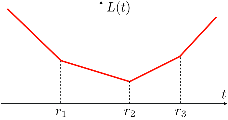
where $L(t)$ is the sum of weighted absolute values

$$L(t)\triangleq\sum_{i=1}^{L}p_{i}|t-r_{i}|.$$

An example of this function is shown in Fig. 1.

Figure 1: Piecewise linear function $L(t)$ in the cost function (7).

As is shown in this figure, the function $L(t)$ is continuous, convex, and piecewise linear. In fact, we have the following proposition:

Proposition 2

The function $L(t)$ is continuous and convex on ${\mathbb{R}}$ and is a piecewise linear function given by

$$L(t)=\begin{cases}-t+\overline{r},&\text{if~{}}t\in(-\infty,r_{1}]\\ a_{i}t+b_{i},&\text{if~{}}t\in(r_{i},r_{i+1}],~{}i=1,2,\ldots,L-1\\ t-\overline{r},&\text{if~{}}t\in[r_{L},\infty).\end{cases}$$

where

$$\overline{r}\triangleq\sum_{i=1}^{L}p_{i}r_{i},$$

$$a_{i}\triangleq\sum_{j=1}^{i}p_{j}-\sum_{j=i+1}^{L}p_{j},~{}~{}b_{i}\triangleq-\sum_{j=1}^{i}p_{j}r_{j}+\sum_{j=i+1}^{L}p_{j}r_{j}.$$

Proof:

Since each function $|t-r_{i}|$ in $L(t)$ is continuous and convex on $\mathbb{R}$, the function $L(t)$, which is the convex combination of $|t-r_{i}|$, $i=1,2,\ldots,L$, is also continuous and convex on $\mathbb{R}$.

Suppose $t\leq r_{1}$. From the inequality (1), we have $t-r_{i}\leq 0$ for $i=1,2,\ldots,L$, and hence

$$L(t)=-\sum_{i=1}^{L}p_{i}(t-r_{i})=-t+\overline{r},$$

where we used (3). Next, suppose $r_{i}<t\leq r_{i+1}$ ($i=1,2,\ldots,L-1$). The inequality (1) gives $t-r_{j}>0$ for $j=1,2,\ldots,i$ and $t-r_{j}\leq 0$ for $j=i+1,i+2,\ldots,L$. It follows that

$$L(t)=\sum_{j=1}^{i}p_{j}(t-r_{j})-\sum_{j=i+1}^{L}p_{j}(t-r_{j})=a_{i}t+b_{i}.$$

Finally, if $t\geq r_{L}$, then $t-r_{i}\geq 0$ for $i=1,2,\ldots,L$ due to (1), and hence

$$L(t)=\sum_{i=1}^{L}p_{i}(t-r_{i})=t-\overline{r}.$$

∎

Note that the function $L(t)$ is rewritten as

$$L(t)=\max_{i=0,1,\ldots,L}\{a_{i}t+b_{i}\},$$

where $a_{0}=-1$, $b_{0}=\overline{r}$, $a_{L}=1$, and $b_{L}=-\overline{r}$. It follows that the optimization (6) is equivalently described as

$$\underset{{\boldsymbol{\theta}}\in{\mathbb{R}}^{N}}{\text{minimize}} {\boldsymbol{1}}_{N}^{\top}{\boldsymbol{\theta}}$$ (8)

subject to $${\boldsymbol{y}}=\Phi{\boldsymbol{z}}, A{\boldsymbol{z}}+{\boldsymbol{b}}\leq E{\boldsymbol{\theta}},$$

where ${\boldsymbol{\theta}}\in{\mathbb{R}}^{N}$ is an auxiliary variable, and

$$\begin{split}A&\triangleq I_{N}\otimes{\boldsymbol{a}}\in{\mathbb{R}}^{N(L+1)\times N},{\boldsymbol{a}}\triangleq[a_{0},a_{1},\ldots,a_{L}]^{\top}\in{\mathbb{R}}^{L+1},\\ {\boldsymbol{b}}&\triangleq{\boldsymbol{1}}_{N}\otimes{\boldsymbol{b}}\in{\mathbb{R}}^{N(L+1)},{\boldsymbol{b}}\triangleq[b_{0},b_{1},\ldots,b_{L}]^{\top}\in{\mathbb{R}}^{L+1},\\ E&\triangleq I_{N}\otimes{\boldsymbol{1}}_{L+1}\in{\mathbb{R}}^{N(L+1)\times N}.\end{split}$$

This is a standard linear programming problem and can be efficiently solved by numerical optimization softwares, such as cvx in MATLAB [11, 12].

Now, we discuss the validity of the relaxation optimization given in (6) or (8). To see this, we extend the notion of the null space property [17] in compressed sensing to our problem:

Definition 1

A matrix $\Phi\in{\mathbb{C}}^{M\times N}$ is said to satisfy the null space property for an alphabet $\mathcal{X}$ if

$$F({\boldsymbol{x}})<F({\boldsymbol{x}}-{\boldsymbol{v}}),$$ (9)

for any ${\boldsymbol{x}}\in{\mathcal{X}}^{N}$ and any ${\boldsymbol{v}}\in{\mathrm{ker}}\,\Phi\setminus\{{\boldsymbol{0}}\}$.

Then we have the following theorem:

Theorem 1

Let $\Phi\in{\mathbb{C}}^{M\times N}$. Every ${\boldsymbol{x}}\in{\mathcal{X}}^{N}$ is uniquely recovered from the $\ell^{1}$ optimization (6) with ${\boldsymbol{y}}=\Phi{\boldsymbol{x}}$ if and only if $\Phi$ satisfies the null space property for $\mathcal{X}$.

Proof:

($\Rightarrow$): Take any ${\boldsymbol{v}}\in{\mathrm{ker}}~{}\Phi\setminus\{0\}$ and ${\boldsymbol{x}}\in{\mathcal{X}}^{N}$. Put ${\boldsymbol{z}}\triangleq{\boldsymbol{x}}-{\boldsymbol{v}}$. Since ${\boldsymbol{v}}\in\mathrm{ker}\,\Phi$, we have $\Phi{\boldsymbol{v}}=\Phi({\boldsymbol{v}}-{\boldsymbol{x}}+{\boldsymbol{x}})={\boldsymbol{0}}$, or $\Phi{\boldsymbol{x}}=\Phi{\boldsymbol{z}}$. This means that ${\boldsymbol{z}}$ is in the feasible set of the optimization problem (6) with ${\boldsymbol{y}}=\Phi{\boldsymbol{x}}$. Also, we have ${\boldsymbol{x}}\neq{\boldsymbol{z}}$ since ${\boldsymbol{v}}\neq{\boldsymbol{0}}$. Now, by assumption, ${\boldsymbol{x}}$ is the unique solution of (6) with ${\boldsymbol{y}}=\Phi{\boldsymbol{x}}$, and hence we have $F({\boldsymbol{x}})<F({\boldsymbol{z}})=F({\boldsymbol{x}}-{\boldsymbol{v}})$.

($\Leftarrow$): Take any ${\boldsymbol{x}}\in{\mathcal{X}}^{N}$ and ${\boldsymbol{z}}\in{\mathbb{C}}^{N}$ such that ${\boldsymbol{x}}\neq{\boldsymbol{z}}$ and $\Phi{\boldsymbol{x}}=\Phi{\boldsymbol{z}}$. Put ${\boldsymbol{v}}\triangleq{\boldsymbol{x}}-{\boldsymbol{z}}$. Then we have ${\boldsymbol{v}}\in\mathrm{ker}\,\Phi\setminus\{0\}$. From the null space property for ${\mathcal{X}}$, we have $F({\boldsymbol{x}})<F({\boldsymbol{x}}-{\boldsymbol{v}})=F({\boldsymbol{z}})$. It follows that ${\boldsymbol{x}}$ is the unique solution of (6). ∎

IV Examples

In this section, we show two examples to illustrate the effectiveness of the proposed method.

The first example is one-dimensional signal reconstruction with multiple symbols. Let the original signal ${\boldsymbol{x}}$ be a $200$-dimensional vector (i.e. $N=200$) and the elements are drawn from the following alphabets with probability distributions:

$$\begin{split}{\mathcal{X}}_{2}&\triangleq\{0,1\}:{\mathbb{P}}(0)=p,~{}{\mathbb{P}}(1)=1-p,\\ {\mathcal{X}}_{3}&\triangleq\{-1,0,1\}:{\mathbb{P}}(0)=p,~{}{\mathbb{P}}(1)={\mathbb{P}}(-1)=\frac{1-p}{2},\\ {\mathcal{X}}_{5}&\triangleq\{-2,-1,0,1,2\}:{\mathbb{P}}(0)=p,\\ &\quad{\mathbb{P}}(-2)={\mathbb{P}}(-1)={\mathbb{P}}(1)={\mathbb{P}}(2)=\frac{1-p}{4},\end{split}$$ (10)

where $p\in[0,1]$. We assume the measurement vector ${\boldsymbol{y}}$ is a $100$-dimensional vector (i.e. $M=100$), and the measurement matrix $\Phi$ is generated such that each element is independently drawn from the Gaussian distribution with a mean of 0 and a standard deviation of $1$ by using a MATLAB command, randn(100,200). The original vector ${\boldsymbol{x}}$ is also generated such that each element is independently drawn from the distribution (10) with varying parameter $p\in[0,1]$.

Figure 2: Averaged NSR $\|{\boldsymbol{x}}-\hat{{\boldsymbol{x}}}\|_{2}/\|{\boldsymbol{x}}\|_{2}$ vs probability $p$ for $\mathcal{X}_{2}$ (top), $\mathcal{X}_{3}$ (middle), $\mathcal{X}_{5}$ (bottom), by the proposed (solid) and the basis pursuit (dash)

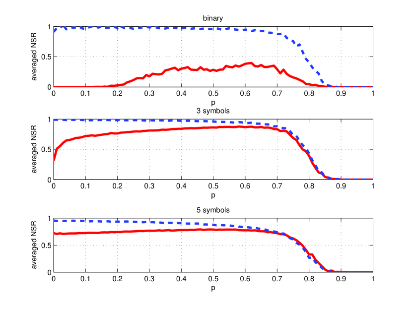
Fig. 2 shows the graphs of the averaged NSR (noise-to-signal ratio) $\|{\boldsymbol{x}}-\hat{{\boldsymbol{x}}}\|_{2}/\|{\boldsymbol{x}}\|_{2}$ for $\mathcal{X}_{2},\mathcal{X}_{3},\mathcal{X}_{5}$ in (10), where $\hat{{\boldsymbol{x}}}$ is the reconstructed signal, with 200 trials of random $\Phi$ and ${\boldsymbol{x}}$ for each $p\in[0,1]$. If $p$ is large (i.e., $p\approx 1$), then the original vector ${\boldsymbol{x}}$ is sparse, and we also reconstruct the original signal by the basis pursuit

$$\min_{{\boldsymbol{z}}\in{\mathbb{R}}^{N}}\|{\boldsymbol{z}}\|_{1}\text{~{}subject to~{}}{\boldsymbol{y}}=\Phi{\boldsymbol{z}},$$

and then round off the values by the basis pursuit to the nearest integer. The error graphs by the basis pursuit are also shown in Fig. 2. For the binary alphabet $\mathcal{X}_{2}=\{0,1\}$, one may exchange the roles of 0 and 1 before performing the basis pursuit, and the error curve below $p=0.5$ is pessimistic. However, such a simple strategy cannot be applied to $\mathcal{X}_{3}$ and $\mathcal{X}_{5}$ for the basis pursuit, while the proposed method works well for small $p$. This is because the basis pursuit does not fully utilize the information of the alphabet (i.e., the basis pursuit only uses the information of the value $0$ through the sparsity). We also note that the basis pursuit can be used only when the alphabet includes $0$, while the proposed method works as well when $0$ is not an element of the alphabet. Fig. 2 also implies a conjecture that the performance of the proposed method converges that of the basis pursuit as the size of the alphabet goes to infinity.

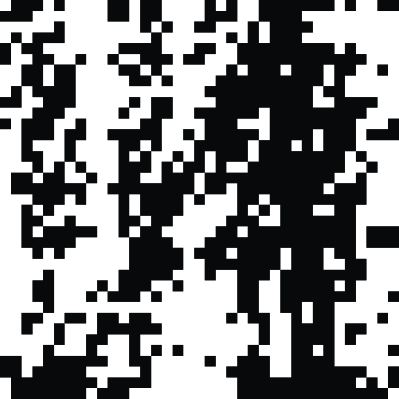
Next, we see an example from image processing. Let us consider a binary (or black-and-white) image shown in Fig. 3 (left), which is a $37\times 37$-pixel binary-valued image. We add random Gaussian noise with a mean of 0 and a standard deviation of $0.1$ to each pixel to obtain a disturbed image as shown in Fig. 3 (right). We represent this disturbed image as a real-valued matrix $X\in{\mathbb{R}}^{37\times 37}$. Then we apply the discrete Fourier transform (DFT) to $X$ to obtain

$$\hat{X}=WXW$$ (11)

where $W$ is the DFT matrix defined by

$$W\triangleq\begin{bmatrix}1&1&1&\ldots&1\\ 1&\omega&\omega^{2}&\ldots&\omega^{K-1}\\ \vdots&\vdots&\vdots&\ddots&\vdots\\ 1&\omega^{K-1}&\omega^{2(K-1)}&\ldots&\omega^{(K-1)(K-1)}\end{bmatrix},$$

where $K=37$ and $\omega\triangleq\exp(-\mathrm{j}2\pi/K)$. The relation can be equivalently represented by

$$\mathrm{vec}(\hat{X})=(W\otimes W)\mathrm{vec}(X)\in\mathbb{C}^{1369}.$$

We then randomly down-sample the vector $\mathrm{vec{(\hat{X})}}$ to obtain a half-sized vector ${\boldsymbol{y}}\in\mathbb{C}^{685}$. The measurement matrix $\Phi$ is then a $685\times 1369$ matrix generated by randomly down-sampling row vectors from $W\otimes W$. Fig. 4 shows the reconstructed images by the basis pursuit with rounding off (left) and by the proposed method (right). For the proposed method, we assumed $\mathbb{P}(0)=\mathbb{P}(1)=1/2$. The results clearly show the effectiveness of our method also for image reconstruction.

Figure 3: Original image (left) and disturbed image by random noise (right)

Figure 4: Reconstructed images by the basis pursuit (left) and by the proposed method (right)

V Conclusion

In this letter, we have proposed a reconstruction method for discrete signals based on the sum of absolute values (or the weighted $\ell^{1}$ norm). The reconstruction algorithm is described as linear programming, which can be solved effectively by numerical optimization softwares. Examples have been shown that the proposed method is much more effective than the basis pursuit which only uses the information of sparsity. Future work includes an accessible condition that ensures the null space property, as the restricted isometry property in compressed sensing.

References

- [1] D. L. Donoho, “Compressed sensing,” IEEE Trans. Inf. Theory, vol. 52, no. 4, pp. 1289–1306, Apr. 2006.
- [2] Y. C. Eldar and G. Kutyniok, Compressed Sensing: Theory and Applications. Cambridge University Press, 2012.
- [3] K. Hayashi, M. Nagahara, and T. Tanaka, “A user’s guide to compressed sensing for communications systems,” IEICE Trans. on Communications, vol. E96-B, no. 3, pp. 685–712, Mar. 2013.
- [4] S. S. Chen, D. L. Donoho, and M. A. Saunders, “Atomic decomposition by basis pursuit,” SIAM J. Sci. Comput., vol. 20, no. 1, pp. 33–61, Aug. 1998.
- [5] Y. C. Pati, R. Rezaiifar, and P. S. Krishnaprasad, “Orthogonal matching pursuit: Recursive function approximation with applications to wavelet decomposition,” in Proc. the 27th Annual Asilomar Conf. on Signals, Systems and Computers, Nov. 1993, pp. 40–44.
- [6] M. Duarte, M. Davenport, D. Takhar, J. Laska, T. Sun, K. Kelly, and R. Baraniuk, “Single-pixel imaging via compressive sampling,” IEEE Signal Process. Mag., vol. 25, no. 2, pp. 83–91, Mar. 2008.
- [7] V. Bioglio, G. Coluccia, and E. Magli, “Sparse image recovery using compressed sensing over finite alphabets,” in Proc. IEEE International Conference on Image Processing (ICIP), Oct. 2014.
- [8] A.-J. van der Veen, S. Talwar, and A. Paulraj, “Blind estimation of multiple digital signals transmitted over FIR channels,” Signal Processing Letters, IEEE, vol. 2, no. 5, pp. 99–102, May 1995.
- [9] B. Knoop, F. Monsees, C. Bockelmann, D. Peters-Drolshagen, S. Paul, and A. Dekorsy, “Compressed sensing K-best detection for sparse multi-user communications,” in Proc. 22nd European Signal Processing Conference (EUSIPCO), Sep. 2014.
- [10] A. Bemporad and M. Morari, “Control of systems integrating logic, dynamics, and constraints,” Automatica, vol. 35, no. 3, pp. 407–427, 1999.
- [11] M. Grant and S. Boyd, “CVX: Matlab software for disciplined convex programming, version 2.1,” http://cvxr.com/cvx, Mar. 2014.
- [12] ——, “Graph implementations for nonsmooth convex programs,” in Recent Advances in Learning and Control, ser. Lecture Notes in Control and Information Sciences, V. Blondel, S. Boyd, and H. Kimura, Eds. Springer, 2008, vol. 371, pp. 95–110.
- [13] Z. Tian, G. Leus, and V. Lottici, “Detection of sparse signals under finite-alphabet constraints,” in Proc. IEEE Int. Conf. Acoust. Speech Signal Process (ICASSP), Apr. 2009, pp. 2349–2352.
- [14] J. Ilic and T. Strohmer, “Sparsity enhanced decision feedback equalization,” IEEE Trans. Signal Process., vol. 60, no. 5, pp. 2422–2432, May 2012.
- [15] S. Sarvotham, D. Baron, and R. G. Baraniuk, “Compressed sensing reconstruction via belief propagation,” 2006.
- [16] A. K. Das and S. Vishwanath, “On finite alphabet compressive sensing,” in Proc. IEEE Int. Conf. Acoust. Speech Signal Process (ICASSP), May 2013, pp. 5890–5894.
- [17] A. Cohen, W. Dahmen, and R. DeVore, “Compressed sensing and best -term approximation,” J. Amer. Math. Soc., no. 22, pp. 211–231, 2009.