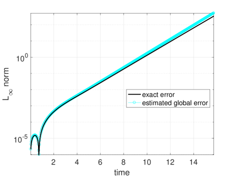
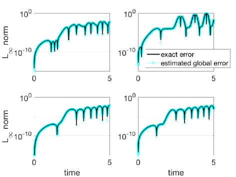
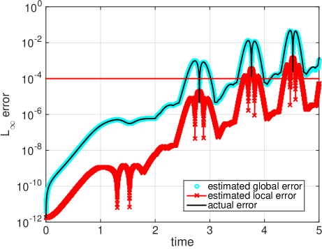
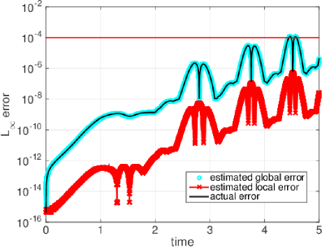
Estimating Global Errors in Time Steppingthanks: This material is based upon work supported by the U.S. Department of Energy, Office of Science, Advanced Scientific Computing Research Program under contract DE-AC02-06CH11357, FWP #56706 and #57K87.

Emil Constantinescu Mathematics and Computer Science Division, Argonne National Laboratory, 9700 S. Cass Avenue, Argonne, IL 60439 (emconsta@mcs.anl.gov).
Abstract

This study introduces new time-stepping strategies with built-in global error estimators. The new methods propagate the defect along with the numerical solution much like solving for the correction or Zadunaisky’s procedure; however, the proposed approach allows for overlapped internal computations and, therefore, represents a generalization of the classical numerical schemes for solving differential equations with global error estimation. The resulting algorithms can be effectively represented as general linear methods. We present a few explicit self-starting schemes akin to Runge-Kutta methods with global error estimation and illustrate the theoretical considerations on several examples.

keywords:
time integration, local and global error estimation, general linear methods
AMS:
65L05, 65L06, 65L20, 65L70

1 Introduction

The global error or a posteriori error represents the actual numerical error resulting after applying a time-stepping algorithm. Calculating this error and controlling it by step-size reduction are generally viewed as expensive processes, and therefore in practice only local error or the error from one step to the next is used for error estimation and control [49, 2, 47, 61]. In general, however, local error estimates cannot predict how those local errors will propagate through the simulation, and for some problems these local errors can grow to be larger than intended. Therefore, from the end-user perspective, local error estimation (LEE) is not always suitable, especially for problems with unstable modes or long integration times [48, 43] because the solution may end up having unexpectedly large numerical errors. This aspect prompts us to revisit global error estimation in order to make it more transparent and practical, which ultimately leads to better error control and reliable accuracy.

In this study we introduce and analyze efficient strategies for estimating global errors for time-stepping algorithms. We present a unifying approach that includes most of the classical strategies as particular cases, and we develop new algorithms that fall under general linear time-stepping schemes. One of the most comprehensive surveys for global error estimation is by Skeel [78]. We focus on a subset of the methods discussed therein and generalize some of the results presented there.

Global error estimation in time stepping has a long history [52, 1, 72, 69, 62, 73, 32, 30, 33, 31, 60, 67, 70, 74, 58, 34, 83, 36]. A posteriori global error estimation has been recently discussed in [21, 37, 54, 3]. Step-size control with multimethod Runge-Kutta (RK) is discussed in [76, 75, 73, 22]. Global error estimation for stiff problems is discussed in [29, 55, 81, 82]. Adjoint methods for global error estimation for PDEs [4, 59] are analyzed in [39, 25]. These studies cover most of the types of strategy that have been proposed to address global error estimation. The Zadunaisky procedure [86] and the related procedure for solving for the correction [78] are arguably the most popular global-error estimation strategies [1, 52]. The work of Dormand et al. [30, 33] relies on this procedure and is extended to a composition of RK methods in [31]. Further extensions are introduced by Murua and Makazaga [63, 60]. Shampine [73] proposes using multiple methods to estimate global errors.

Recent work on global error control by Kulikov, Weiner, et al. [85, 56, 57] extends the quasi-consistency property introduced by Skeel [77] and recently advanced by Kulikov [53]. Moreover, these ideas were extended to peer methods by using a peer-triplets strategy by Weiner and Kulikov [84]. These strategies seem to give very good results in terms of global error control on prototypical problems. The general linear (GL)-based algorithm proposed in this study bears a more general representation of the methods discussed above. We will also show how Runge-Kutta triplets [33] and by proxy the peer triplets [84] are naturally represented as GL methods.

Our work builds on similar ideas introduced by Shampine [73] and Zadunaisky [86] and the followups in the sense that the strategy evolves the defect along with the solution; however, in our strategy the internal calculations of the two quantities can be overlapped by using a single scheme to evolve them simultaneously. Therefore, the new method automatically integrates the local truncation error or defect. Previous strategies can be cast as particular cases of the one introduced in this study when the overlapping part is omitted. This leads to new types of schemes that are naturally represented as GL methods, which are perfectly suited for this strategy, as we demonstrate.

The general linear methods introduced in this study have built-in asymptotically correct global and local error estimators. These methods propagate at least two quantities; one of them is the solution, and the other one can be either the global error or equivalently another solution that can be used to determine the global errors. We show that two new elements are required for GL methods to propagate global errors: (i)𝑖(i) a particular relation between the truncation error of the two quantities and (ii)𝑖𝑖(ii) a decoupling property between the errors of its two outputs. The GL framework encapsulates all linear time-stepping algorithms and provides a platform for robust algorithms with built-in error estimates. Moreover, this encapsulated treatment simplifies the analysis of compound schemes used for global error analysis; for instance, stability analysis turns out to be much simpler in this representation.

We consider the first-order system of nonautonomous ordinary differential equations

(1) y(t)=f(t,y(t));y(t0)=y0,t0<tT,ym,f:m+1m,\displaystyle y(t)^{\prime}=f(t,y(t))\,;~{}y(t_{0})=y_{0}\,,~{}t_{0}<t\leq T\,,~{}y\in\mathbb{R}^{m},f:\mathbb{R}^{m+1}\rightarrow\mathbb{R}^{m}\,,

of size m𝑚m with y0subscript𝑦0y_{0} given. We will use the tensor notation denoting the components in (1) by y{j}superscript𝑦𝑗y^{\{j\}} and f{j}superscript𝑓𝑗f^{\{j\}}, j=1, 2,,m𝑗12𝑚j=1,\,2,\,\dots,\,m. We will often consider nonautonomous systems because the exposition is less cluttered. In order to convert (1) to autonomous form, the system can be augmented with (y{m+1})=1superscriptsuperscript𝑦𝑚11(y^{\{m+1\}})^{\prime}=1, with y{m+1}(t0)=t0superscript𝑦𝑚1subscript𝑡0subscript𝑡0y^{\{m+1\}}(t_{0})=t_{0}; hence, t=y{m+1}(t)𝑡superscript𝑦𝑚1𝑡t=y^{\{m+1\}}(t). This is likely not a restrictive theoretical assumption, but there can be exceptions [64]; however, in practice it is preferable to treat the temporal components separately. For brevity, we will refer to (1) in both autonomous and nonautonomous forms depending on the context.

The purpose of this study is to analyze strategies for estimating the global error at every time step n𝑛n,

(2) ε(tn)=y(tn)yn,n=1,2,,NT,formulae-sequence𝜀subscript𝑡𝑛𝑦subscript𝑡𝑛subscript𝑦𝑛𝑛12subscript𝑁𝑇\displaystyle\varepsilon(t_{n})=y(t_{n})-y_{n}\,,~{}n=1,2,\dots,N_{T}\,,

that is, the difference between the exact solution y(tn)𝑦subscript𝑡𝑛y(t_{n}) and a numerical approximation ynsubscript𝑦𝑛y_{n} from a sequence of NTsubscript𝑁𝑇N_{T} steps. A priori and a posteriori error bounds under appropriate smoothness assumptions are well known [46, 43]. This study focuses on efficient a posteriori estimates of ε(tn)𝜀subscript𝑡𝑛\varepsilon(t_{n}).

This study has several limitations. Stiff differential equations are not directly addressed. Although the theory presented here, more precisely the consistency result, applies to the stiff case; however, additional constraints are believed to be necessary to preserve the asymptotic correctness of the error estimators. Moreover, we do not discuss global error control. Although algorithms introduced in this study work well with variable time steps as we illustrate through the results in Fig. 8, we do not address error control strategies here. This is a topic for a future study; however, local error control can be used as before with global error estimates being a diagnostic of the output.

We aim to bring a self-contained view of global error estimation. New results are interlaced with classical theory to provide a contained picture for this topic. We also illustrate the connection among different strategies. The proposed algorithm generalizes all the strategies reviewed in this study and provides a robust instrument for estimating a posteriori errors in numerical integration. Section 2 introduces the background for the theoretical developments and discusses different strategies to estimate the global errors, which include developments that form the basis of the proposed approach. In Sec. 3 we discuss the general linear methods that are used to represent practical algorithms. The analysis of these schemes and examples are provided in Sec. 4. In Sec. 5 we discuss the relationship between the approach introduced here and related strategies and show how the latter are particular instantiations of the former. Several numerical experiments are presented in Sec. 6, and concluding remarks are discussed in Sec. 7.

2 Global error estimation

Let us consider a one-step linear numerical discretization method for (1),

(3) yn+1=yn+ΔtΦ(tn,yn,Δtn),y0=y(t0),n=1,2,,NT,formulae-sequencesubscript𝑦𝑛1subscript𝑦𝑛Δ𝑡Φsubscript𝑡𝑛subscript𝑦𝑛Δsubscript𝑡𝑛formulae-sequencesubscript𝑦0𝑦subscript𝑡0𝑛12subscript𝑁𝑇\displaystyle y_{n+1}=y_{n}+{\Delta t}\Phi(t_{n},y_{n},{\Delta t}_{n})\,,~{}y_{0}=y(t_{0})\,,~{}n=1,2,\dots,N_{T}\,,

where ΦΦ\Phi is called the Taylor increment function with Φ(tn,yn,0)=f(tn,yn)Φsubscript𝑡𝑛subscript𝑦𝑛0𝑓subscript𝑡𝑛subscript𝑦𝑛\Phi(t_{n},y_{n},0)=f(t_{n},y_{n}). We denote the time series obtained via (3) with step ΔtΔ𝑡{\Delta t} by {yΔt}subscript𝑦Δ𝑡\{y_{\Delta t}\}. A method of order p𝑝p for a sufficiently smooth function f𝑓f satisfies

(4a) y(tn+Δt)yn+1C1Δtp+1,yn=y(tn),formulae-sequencenorm𝑦subscript𝑡𝑛Δ𝑡subscript𝑦𝑛1subscript𝐶1Δsuperscript𝑡𝑝1subscript𝑦𝑛𝑦subscript𝑡𝑛\displaystyle||y(t_{n}+{\Delta t})-y_{n+1}||\leq C_{1}{\Delta t}^{p+1}\,,y_{n}=y(t_{n})\,,
for a constant C1subscript𝐶1C_{1}. The local error then satisfies
(4b) y(t+Δt)y(t)ΔtΦ(t,y(t),Δt)=dp+1(t)Δtp+1+𝒪(Δtp+2).𝑦𝑡Δ𝑡𝑦𝑡Δ𝑡Φ𝑡𝑦𝑡Δ𝑡subscript𝑑𝑝1𝑡Δsuperscript𝑡𝑝1𝒪Δsuperscript𝑡𝑝2\displaystyle y(t+{\Delta t})-y(t)-{\Delta t}\Phi(t,y(t),{\Delta t})=d_{p+1}(t){\Delta t}^{p+1}+{\mathcal{O}}({\Delta t}^{p+2})\,.

The following classical result states the bounds on the global errors.

Theorem 1.

Let U𝑈U be a neighborhood of {(t,y(t))|t0tT}conditional-set𝑡𝑦𝑡subscript𝑡0𝑡𝑇\{(t,y(t))|t_{0}\leq t\leq T\}, where y(t)𝑦𝑡y(t) is the exact solution of (1) and there exists a constant L𝐿L such that f(t,y)f(t,z)Lyznorm𝑓𝑡𝑦𝑓𝑡𝑧𝐿norm𝑦𝑧||f(t,y)-f(t,z)||\leq L||y-z|| and (4) is satisfied for (t,x)𝑡𝑥(t,x), (t,y)U𝑡𝑦𝑈(t,y)\in U. Then

(5) ε(t)ΔtpC2L(eL(tt0)1)norm𝜀𝑡Δsuperscript𝑡𝑝subscript𝐶2𝐿superscript𝑒𝐿𝑡subscript𝑡01\displaystyle||\varepsilon(t)||\leq{\Delta t}^{p}\frac{C_{2}}{L}\left(e^{L(t-t_{0})}-1\right)\,

for a constant C2subscript𝐶2C_{2}.

This is proved in several treatises [46, 79, 43]. Under sufficient smoothness assumptions [46, 42], it follows that the global error satisfies

(6) ε(t)=y(t)yΔt(t)=ep(t)Δtp+o(Δtp),𝜀𝑡𝑦𝑡subscript𝑦Δ𝑡𝑡subscript𝑒𝑝𝑡Δsuperscript𝑡𝑝𝑜Δsuperscript𝑡𝑝\displaystyle\varepsilon(t)=y(t)-y_{{\Delta t}}(t)=e_{p}(t){\Delta t}^{p}+{o}({\Delta t}^{p})\,,

where yn:=yΔt(t)assignsubscript𝑦𝑛subscript𝑦Δ𝑡𝑡y_{n}:=y_{{\Delta t}}(t) at t=t0+nΔt𝑡subscript𝑡0𝑛Δ𝑡t=t_{0}+n{\Delta t}. These results are obtained by comparing the expansions of the exact and the numerical solutions. To alleviate the analysis difficulties that come with large p𝑝p, we use the B-series representation of the derivatives.

Definition 2 (Rooted trees and labeled trees [6, 24]).

Let 𝒯𝒯{\mathcal{T}} be a set of ordered indexes 𝒯q={j1<j2<j3<<jq}subscript𝒯𝑞subscript𝑗1subscript𝑗2subscript𝑗3subscript𝑗𝑞{\mathcal{T}}_{q}=\{j_{1}<j_{2}<j_{3}<\cdots<j_{q}\} with cardinality q𝑞q. A labeled tree of order q𝑞q is a mapping τ:𝒯q\{j1}𝒯q:𝜏\subscript𝒯𝑞subscript𝑗1subscript𝒯𝑞{\tau}:{\mathcal{T}}_{q}\backslash\{j_{1}\}\rightarrow{\mathcal{T}}_{q} such that τ(j)<j𝜏𝑗𝑗{\tau}(j)<j, j𝒯q\{j1}for-all𝑗\subscript𝒯𝑞subscript𝑗1\forall j\in{\mathcal{T}}_{q}\backslash\{j_{1}\}. The set of all labeled trees of order q𝑞q is denoted by LTq𝐿subscript𝑇𝑞{LT}_{q}. The order of a tree is denoted by ρ(τ)=q𝜌𝜏𝑞{\rho}({\tau})=q. Furthermore, we define an equivalence class of order q𝑞q as the permutation σ:𝒯q𝒯q:𝜎subscript𝒯𝑞subscript𝒯𝑞\sigma:{\mathcal{T}}_{q}\rightarrow{\mathcal{T}}_{q} such that σ(j)=j𝜎𝑗𝑗\sigma(j)=j, τkσ=στsubscript𝜏𝑘𝜎𝜎subscript𝜏{\tau}_{k}\sigma=\sigma{\tau}_{\ell}, τk,τLTqsubscript𝜏𝑘subscript𝜏𝐿subscript𝑇𝑞{\tau}_{k},{\tau}_{\ell}\in{LT}_{q}. These unlabeled trees of order q𝑞q are denoted by Tqsubscript𝑇𝑞{T}_{q}, and the number of different monotonic labelings of τTq𝜏subscript𝑇𝑞{\tau}\in{T}_{q} is denoted by α(τ)𝛼𝜏\alpha({\tau}). Also, Tq#=Tqsuperscriptsubscript𝑇𝑞#subscript𝑇𝑞{T}_{q}^{\#}={T}_{q}\cup{\emptyset}, where \emptyset is the empty tree and the only one with ρ()=0𝜌0{\rho}(\emptyset)=0.

Definition 3 (Elementary differentials [6, 24]).

For a labeled tree τLTq𝜏𝐿subscript𝑇𝑞{\tau}\in{LT}_{q} we call an elementary differential the expression

(7) F{K1}(τ)(y)=K2,K3,,Kqi=1qfτ1(Ki){Ki},superscript𝐹subscript𝐾1𝜏𝑦subscriptsubscript𝐾2subscript𝐾3subscript𝐾𝑞superscriptsubscriptproduct𝑖1𝑞subscriptsuperscript𝑓subscript𝐾𝑖superscript𝜏1subscript𝐾𝑖\displaystyle F^{\{K_{1}\}}({\tau})(y)=\sum_{K_{2},K_{3},\dots,K_{q}}\prod_{i=1}^{q}f^{\{K_{i}\}}_{{\tau}^{-1}(K_{i})}\,,

where K1,K2,,Kq=1,2,,mformulae-sequencesubscript𝐾1subscript𝐾2subscript𝐾𝑞12𝑚K_{1},K_{2},\dots,K_{q}=1,2,\dots,m, and fK1,K2,,Kr{J}=rf{J}/y{K1}y{K2}y{Kr}subscriptsuperscript𝑓𝐽subscript𝐾1subscript𝐾2subscript𝐾𝑟superscript𝑟superscript𝑓𝐽superscript𝑦subscript𝐾1superscript𝑦subscript𝐾2superscript𝑦subscript𝐾𝑟f^{\{J\}}_{K_{1},K_{2},\dots,K_{r}}=\partial^{r}f^{\{J\}}/\partial y^{\{K_{1}\}}y^{\{K_{2}\}}\dots y^{\{K_{r}\}}. We denote by F(τ)(y)=[F{1}(τ)(y),F{2}(τ)(y),,F{m}(τ)(y)]T𝐹𝜏𝑦superscriptsuperscript𝐹1𝜏𝑦superscript𝐹2𝜏𝑦superscript𝐹𝑚𝜏𝑦𝑇F({\tau})(y)=[F^{\{1\}}({\tau})(y),F^{\{2\}}({\tau})(y),\dots,F^{\{m\}}({\tau})(y)]^{T}.

We use the graphical notation to represent derivatives discussed in [15, 43].

Example

The tree corresponds to ff′′(f,f)superscript𝑓superscript𝑓′′𝑓𝑓f^{\prime}f^{\prime\prime}(f,f). The trees of order 4 are T4={,,,}subscript𝑇4{T}_{4}=\left\{\begin{pspicture}(0.0pt,0.0pt)(12.0pt,18.0pt){\psdot(5.0pt,0.0pt)}{\psdot(5.0pt,6.0pt)}{\psdot(0.0pt,6.0pt)}{\psdot(10.0pt,6.0pt)}{\psline(5.0pt,0.0pt)(5.0pt,6.0pt)}{\psline(5.0pt,0.0pt)(0.0pt,6.0pt)}{\psline(5.0pt,0.0pt)(10.0pt,6.0pt)}\end{pspicture},\begin{pspicture}(0.0pt,0.0pt)(12.0pt,18.0pt){\psdot(5.0pt,0.0pt)}{\psdot(5.0pt,12.0pt)}{\psdot(0.0pt,6.0pt)}{\psdot(10.0pt,6.0pt)}{\psline(5.0pt,0.0pt)(10.0pt,6.0pt)}{\psline(10.0pt,6.0pt)(5.0pt,12.0pt)}{\psline(5.0pt,0.0pt)(0.0pt,6.0pt)}\end{pspicture},\begin{pspicture}(0.0pt,0.0pt)(12.0pt,18.0pt){\psdot(5.0pt,0.0pt)}{\psdot(5.0pt,6.0pt)}{\psdot(0.0pt,12.0pt)}{\psdot(10.0pt,12.0pt)}{\psline(5.0pt,0.0pt)(5.0pt,6.0pt)}{\psline(5.0pt,6.0pt)(0.0pt,12.0pt)}{\psline(5.0pt,6.0pt)(10.0pt,12.0pt)}\end{pspicture},\begin{pspicture}(0.0pt,0.0pt)(12.0pt,18.0pt){\psdot(5.0pt,0.0pt)}{\psdot(5.0pt,5.0pt)}{\psdot(5.0pt,10.0pt)}{\psdot(5.0pt,15.0pt)}{\psline(5.0pt,0.0pt)(5.0pt,5.0pt)}{\psline(5.0pt,5.0pt)(5.0pt,10.0pt)}{\psline(5.0pt,10.0pt)(5.0pt,15.0pt)}\end{pspicture}\right\}, α(τ)=1𝛼𝜏1\alpha({\tau})=1 for τT4\{}𝜏\subscript𝑇4{\tau}\in{T}_{4}\backslash\left\{\begin{pspicture}(0.0pt,0.0pt)(12.0pt,18.0pt){\psdot(5.0pt,0.0pt)}{\psdot(5.0pt,12.0pt)}{\psdot(0.0pt,6.0pt)}{\psdot(10.0pt,6.0pt)}{\psline(5.0pt,0.0pt)(10.0pt,6.0pt)}{\psline(10.0pt,6.0pt)(5.0pt,12.0pt)}{\psline(5.0pt,0.0pt)(0.0pt,6.0pt)}\end{pspicture}\right\}, α()=3𝛼3\alpha\left(\begin{pspicture}(0.0pt,0.0pt)(12.0pt,18.0pt){\psdot(5.0pt,0.0pt)}{\psdot(5.0pt,12.0pt)}{\psdot(0.0pt,6.0pt)}{\psdot(10.0pt,6.0pt)}{\psline(5.0pt,0.0pt)(10.0pt,6.0pt)}{\psline(10.0pt,6.0pt)(5.0pt,12.0pt)}{\psline(5.0pt,0.0pt)(0.0pt,6.0pt)}\end{pspicture}\right)=3.

Definition 4 (B-series [45]).

Let a:T:𝑎𝑇a:{T}\rightarrow\mathbb{R} be a mapping between the tree set and real numbers. The following is called a B-series:

B(a,y)𝐵𝑎𝑦\displaystyle B(a,y) =a()y+Δta()f(y)+Δt22a()F()(y)+absent𝑎𝑦Δ𝑡𝑎𝑓𝑦Δsuperscript𝑡22𝑎𝐹𝑦\displaystyle=a(\emptyset)y+{\Delta t}\,a(\begin{pspicture}(0.0pt,0.0pt)(12.0pt,12.0pt){\psdot(5.0pt,6.0pt)}\end{pspicture})f(y)+\frac{{\Delta t}^{2}}{2}a(\begin{pspicture}(0.0pt,0.0pt)(12.0pt,12.0pt){\psdot(5.0pt,0.0pt)}{\psdot(5.0pt,6.0pt)}{\psline(5.0pt,0.0pt)(5.0pt,6.0pt)}\end{pspicture})F(\begin{pspicture}(0.0pt,0.0pt)(12.0pt,12.0pt){\psdot(5.0pt,0.0pt)}{\psdot(5.0pt,6.0pt)}{\psline(5.0pt,0.0pt)(5.0pt,6.0pt)}\end{pspicture})(y)+\cdots
(8) =τTΔtρ(τ)α(τ)ρ(τ)!a(τ)F(τ)(y),absentsubscript𝜏𝑇Δsuperscript𝑡𝜌𝜏𝛼𝜏𝜌𝜏𝑎𝜏𝐹𝜏𝑦\displaystyle=\sum_{{\tau}\in{T}}\frac{{\Delta t}^{{\rho}({\tau})}\alpha({\tau})}{{\rho}({\tau})!}a({\tau})F({\tau})(y)\,,

where T={}T1T2𝑇subscript𝑇1subscript𝑇2{T}=\{\emptyset\}\bigcup{T}_{1}\bigcup{T}_{2}\bigcup\cdots.

The exact solution of an ODE system is a B-series [45]. Formally we have the following result.

Theorem 5 (Exact solution as B-series[45]).

The exact solution of (1)satisfies

y(q)(τ)=τTα(τ)F(τ)(y).superscript𝑦𝑞𝜏subscript𝜏𝑇𝛼𝜏𝐹𝜏𝑦\displaystyle y^{(q)}({\tau})=\sum_{{\tau}\in{T}}\alpha({\tau})F({\tau})(y)\,.

Therefore the exact solution is given by (8) with a(τ)=1𝑎𝜏1a({\tau})=1, and the coefficient of Δtρ(τ)F(τ)(y)Δsuperscript𝑡𝜌𝜏𝐹𝜏𝑦{\Delta t}^{{\rho}({\tau})}F({\tau})(y) in the expansion is given by α(τ)ρ(τ)!𝛼𝜏𝜌𝜏\frac{\alpha({\tau})}{{\rho}({\tau})!}, τTkfor-all𝜏subscript𝑇𝑘\forall{\tau}\in{T}_{k}, k=1,2,,p𝑘12𝑝k=1,2,\dots,p.

The elementary weights in the expression of the B-series are independent. The following result captures this aspect.

Lemma 6 (Independence of elemetary differentials [15]).

The elementary differentials are independent. Moreover, the values of the distinct elementary differentials for (y{j})=j=1k(y{j})mj/mj!superscriptsuperscript𝑦𝑗superscriptsubscriptproduct𝑗1𝑘superscriptsuperscript𝑦𝑗subscript𝑚𝑗subscript𝑚𝑗(y^{\{j\}})^{\prime}=\prod_{j=1}^{k}(y^{\{j\}})^{m_{j}}/m_{j}!, y{j}(t0)=0superscript𝑦𝑗subscript𝑡00y^{\{j\}}(t_{0})=0 are given by F(τi)(y(t0))=ei𝐹subscript𝜏𝑖𝑦subscript𝑡0subscript𝑒𝑖F({\tau}_{i})(y(t_{0}))=e_{i}, where k𝑘k is the number of resulting trees when the root is removed and mjsubscript𝑚𝑗m_{j} is the number of copies of τjsubscript𝜏𝑗{\tau}_{j}.

The order of the numerical method can be defined in terms of a B-series as follows.

Definition 7 (Order of time-stepping methods).

A numerical method applied to (1) with f𝑓f p𝑝p-times continuous differentiable is of order p𝑝p if the expansion of the numerical solution satisfies (8) with ρ(τ)p𝜌𝜏𝑝{\rho}({\tau})\leq p.

2.1 Error equation

We now analyze the propagation of numerical errors through the time-stepping processes.

Theorem 8 (Asymptotic expansion of the global errors [46, 43]).

Suppose that method (3) possesses an expansion (4b) under smoothness conditions of Theorem 1. Then the global error has an asymptotic expansion of form

(9) y(t)yΔt(t)=ep(t)Δtp++eN(t)ΔtN+EΔt(t)ΔtN+1,𝑦𝑡subscript𝑦Δ𝑡𝑡subscript𝑒𝑝𝑡Δsuperscript𝑡𝑝subscript𝑒𝑁𝑡Δsuperscript𝑡𝑁subscript𝐸Δ𝑡𝑡Δsuperscript𝑡𝑁1\displaystyle y(t)-y_{\Delta t}(t)=e_{p}(t){\Delta t}^{p}+\dots+e_{N}(t){\Delta t}^{N}+E_{\Delta t}(t){\Delta t}^{N+1}\,,

where EΔt(t)subscript𝐸Δ𝑡𝑡E_{\Delta t}(t) is bounded on t0<tTsubscript𝑡0𝑡𝑇t_{0}<t\leq T and 0ΔtΔT0Δ𝑡Δ𝑇0\leq{\Delta t}\leq{\Delta T} for some ΔTΔ𝑇{\Delta T}, and ep(t)subscript𝑒𝑝𝑡e_{p}(t) satisfies

(10) ep(t)=fy(t,y)ep(t)+dp+1(t),ep(t0)=0.formulae-sequencesuperscriptsubscript𝑒𝑝𝑡𝑓𝑦𝑡𝑦subscript𝑒𝑝𝑡subscript𝑑𝑝1𝑡subscript𝑒𝑝subscript𝑡00\displaystyle e_{p}^{\prime}(t)=\frac{\partial f}{\partial y}(t,y)\cdot e_{p}(t)+d_{p+1}(t)\,,\quad e_{p}(t_{0})=0\,.

The other ej(t)subscript𝑒𝑗𝑡e_{j}(t) terms satisfy similar equations.

Proof.

Consider a perturbed method y^Δt(t):=yΔt(t)+ep(t)Δtpassignsubscript^𝑦Δ𝑡𝑡subscript𝑦Δ𝑡𝑡subscript𝑒𝑝𝑡Δsuperscript𝑡𝑝\widehat{y}_{{\Delta t}}(t):=y_{{\Delta t}}(t)+e_{p}(t){\Delta t}^{p}. Then y^Δt(t)subscript^𝑦Δ𝑡𝑡\widehat{y}_{{\Delta t}}(t) can be represented as the numerical solution of a new method: y^n+1=y^n+ΔtΦ^(tn,y^n,Δt)subscript^𝑦𝑛1subscript^𝑦𝑛Δ𝑡^Φsubscript𝑡𝑛subscript^𝑦𝑛Δ𝑡\widehat{y}_{n+1}=\widehat{y}_{n}+{\Delta t}\widehat{\Phi}(t_{n},\widehat{y}_{n},{\Delta t}). By comparison with (3) we obtain {y^n}subscript^𝑦𝑛\{\widehat{y}_{n}\},

(11) Φ^(t,y^n,Δt)^Φ𝑡subscript^𝑦𝑛Δ𝑡\displaystyle\widehat{\Phi}(t,\widehat{y}_{n},{\Delta t}) =Φ(tn,y^nep(tn)Δtp,Δt)+(ep(tn+Δt)ep(tn))Δtp1.absentΦsubscript𝑡𝑛subscript^𝑦𝑛subscript𝑒𝑝subscript𝑡𝑛Δsuperscript𝑡𝑝Δ𝑡subscript𝑒𝑝subscript𝑡𝑛Δ𝑡subscript𝑒𝑝subscript𝑡𝑛Δsuperscript𝑡𝑝1\displaystyle=\Phi(t_{n},\widehat{y}_{n}-e_{p}(t_{n}){\Delta t}^{p},{\Delta t})+(e_{p}(t_{n}+{\Delta t})-e_{p}(t_{n})){\Delta t}^{p-1}\,.

Expanding the local error of the perturbed method with the Taylor function defined by (11) yields in general

y(t+Δt)y(t)ΔtΦ^(t,y(t),Δt)𝑦𝑡Δ𝑡𝑦𝑡Δ𝑡^Φ𝑡𝑦𝑡Δ𝑡\displaystyle y(t+{\Delta t})-y(t)-{\Delta t}\widehat{\Phi}(t,y(t),{\Delta t})
(12) =(dp+1(t)+fy(t,y)ep(t)ep(t))Δtp+1+𝒪(Δtp+2).absentsubscript𝑑𝑝1𝑡𝑓𝑦𝑡𝑦subscript𝑒𝑝𝑡superscriptsubscript𝑒𝑝𝑡Δsuperscript𝑡𝑝1𝒪Δsuperscript𝑡𝑝2\displaystyle\qquad=\left(d_{p+1}(t)+\frac{\partial f}{\partial y}(t,y)e_{p}(t)-e_{p}^{\prime}(t)\right){\Delta t}^{p+1}+{\mathcal{O}}({\Delta t}^{p+2})\,.

We take ep(t)subscript𝑒𝑝𝑡e_{p}(t) to satisfy (10), so that by Theorem 1 it follows that

(13) y(t)yΔt(t)=ep(t)Δtp+𝒪(Δtp+1)𝑦𝑡subscript𝑦Δ𝑡𝑡subscript𝑒𝑝𝑡Δsuperscript𝑡𝑝𝒪Δsuperscript𝑡𝑝1\displaystyle y(t)-y_{{\Delta t}}(t)=e_{p}(t){\Delta t}^{p}+{\mathcal{O}}({\Delta t}^{p+1})\,

determines the asymptotic expansion. For more details see [43]. ∎

Equations for the next terms in the global error expansion can be obtained by using the same procedure; however, this is not pursued in this study.

2.1.1 Estimating global errors using two methods

We now introduce the general global error estimation strategy used in this study. This approach relies on propagating two solutions through a linear time-stepping process that has the property of maintaining a fixed ratio between the truncation error terms. This result will play a crucial role in constructing the new methods discussed in Sec. 4 and can be stated as follows.

Theorem 9 (Global error estimation with two methods).

Consider numerical solutions {yn}subscript𝑦𝑛\{y_{n}\} and {y~n}subscript~𝑦𝑛\{\tilde{y}_{n}\} of (1) obtained by two time-stepping methods started from the same exact initial condition under the conditions of Theorem 8. If the local errors of the two methods with increments ΦΦ\Phi and Φ~~Φ\tilde{\Phi} satisfy

(14a) y(t+Δt)y(t)ΔtΦ(t,y(t),Δt)𝑦𝑡Δ𝑡𝑦𝑡Δ𝑡Φ𝑡𝑦𝑡Δ𝑡\displaystyle y(t+{\Delta t})-y(t)-{\Delta t}\Phi(t,y(t),{\Delta t}) =dp+1(tn)Δtp+1+𝒪(Δtp+2),absentsubscript𝑑𝑝1subscript𝑡𝑛Δsuperscript𝑡𝑝1𝒪Δsuperscript𝑡𝑝2\displaystyle=d_{p+1}(t_{n}){\Delta t}^{p+1}+{\mathcal{O}}({\Delta t}^{p+2})\,,
(14b) y(t+Δt)y(t)ΔtΦ~(t,y(t),Δt)𝑦𝑡Δ𝑡𝑦𝑡Δ𝑡~Φ𝑡𝑦𝑡Δ𝑡\displaystyle y(t+{\Delta t})-y(t)-{\Delta t}\tilde{\Phi}(t,y(t),{\Delta t}) =γdp+1(tn)Δtp+1+𝒪(Δtp+2),absent𝛾subscript𝑑𝑝1subscript𝑡𝑛Δsuperscript𝑡𝑝1𝒪Δsuperscript𝑡𝑝2\displaystyle=\gamma d_{p+1}(t_{n}){\Delta t}^{p+1}+{\mathcal{O}}({\Delta t}^{p+2})\,,

where dp+1(tn)=1(p+1)!τTp+1α(τ)a(τ)F(τ)(yn)subscript𝑑𝑝1subscript𝑡𝑛1𝑝1subscript𝜏subscript𝑇𝑝1𝛼𝜏𝑎𝜏𝐹𝜏subscript𝑦𝑛d_{p+1}(t_{n})=\frac{1}{(p+1)!}\sum_{{\tau}\in{T}_{p+1}}\alpha({\tau})a({\tau})F({\tau})(y_{n}) with constant γ1𝛾1\gamma\neq 1, then the global error can be estimated as

(15) εp(tn)=11γ(y~nyn)=ep(tn)Δtp+𝒪(Δtp+1)=ε(tn)+O(Δtp+1),subscript𝜀𝑝subscript𝑡𝑛11𝛾subscript~𝑦𝑛subscript𝑦𝑛subscript𝑒𝑝subscript𝑡𝑛Δsuperscript𝑡𝑝𝒪Δsuperscript𝑡𝑝1𝜀subscript𝑡𝑛𝑂Δsuperscript𝑡𝑝1\displaystyle\varepsilon_{p}(t_{n})=\frac{1}{1-\gamma}\left(\tilde{y}_{n}-y_{n}\right)=e_{p}(t_{n}){\Delta t}^{p}+{\mathcal{O}}({\Delta t}^{p+1})=\varepsilon(t_{n})+O({\Delta t}^{p+1})\,,

when y0=y~0=y(t0)subscript𝑦0subscript~𝑦0𝑦subscript𝑡0y_{0}=\tilde{y}_{0}=y(t_{0}); hence, εny(tn)ynasymptotically-equalssubscript𝜀𝑛𝑦subscript𝑡𝑛subscript𝑦𝑛\varepsilon_{n}\asymp y(t_{n})-y_{n}.

Proof.

Use (9) and (10) to write the global error equations for the two methods with nearby solutions:

(16a) ep(t)superscriptsubscript𝑒𝑝𝑡\displaystyle e_{p}^{\prime}(t) =fy(t,y)ep(t)+dp+1(t),ep(t0)=0,formulae-sequenceabsent𝑓𝑦𝑡𝑦subscript𝑒𝑝𝑡subscript𝑑𝑝1𝑡subscript𝑒𝑝subscript𝑡00\displaystyle=\frac{\partial f}{\partial y}(t,y)\cdot e_{p}(t)+d_{p+1}(t)\,,\quad e_{p}(t_{0})=0\,,
(16b) e~p(t)superscriptsubscript~𝑒𝑝𝑡\displaystyle\tilde{e}_{p}^{\prime}(t) =fy(t,y)e~p(t)+γdp+1(t),e~p(t0)=0.formulae-sequenceabsent𝑓𝑦𝑡𝑦subscript~𝑒𝑝𝑡𝛾subscript𝑑𝑝1𝑡subscript~𝑒𝑝subscript𝑡00\displaystyle=\frac{\partial f}{\partial y}(t,y)\cdot\tilde{e}_{p}(t)+\gamma d_{p+1}(t)\,,\quad\tilde{e}_{p}(t_{0})=0\,.

It follows that the solutions of the two ordinary differential equations satisfy γep(t)=e~p(t)𝛾subscript𝑒𝑝𝑡subscript~𝑒𝑝𝑡\gamma e_{p}(t)=\tilde{e}_{p}(t). We can then verify (15) by inserting (13):

εp(tn)subscript𝜀𝑝subscript𝑡𝑛\displaystyle\varepsilon_{p}(t_{n}) =11γ(y~nyn)absent11𝛾subscript~𝑦𝑛subscript𝑦𝑛\displaystyle=\frac{1}{1-\gamma}\left(\tilde{y}_{n}-y_{n}\right)
=11γ(y(tn)e~p(tn)Δtpy(t)+ep(tn)Δtp+𝒪(Δtp+1))\displaystyle=\frac{1}{1-\gamma}\left(y(t_{n})-\tilde{e}_{p}(t_{n}){\Delta t}^{p}-y(t_{)}+e_{p}(t_{n}){\Delta t}^{p}+{\mathcal{O}}({\Delta t}^{p+1})\right)
=ep(tn)Δtp+𝒪(Δtp+1)absentsubscript𝑒𝑝subscript𝑡𝑛Δsuperscript𝑡𝑝𝒪Δsuperscript𝑡𝑝1\displaystyle=e_{p}(t_{n}){\Delta t}^{p}+{\mathcal{O}}({\Delta t}^{p+1})

for n=1,2,𝑛12n=1,2,\dots. ∎

We will refer to ε𝜀\varepsilon as the exact global error and to εpsubscript𝜀𝑝\varepsilon_{p} as the order-p𝑝p global error estimate. A particular case is γ=0𝛾0\gamma=0. Moreover, under the assumptions of Theorem 9, one can always compute a higher-order approximation by combining the two solutions.

Corollary 10.

If γ=0𝛾0\gamma=0 in Theorem 9, then we revert to the case of using two methods of different orders, p𝑝p and p+1𝑝1p+1, to estimate the global errors for the method of order p𝑝p.

Corollary 11.

A method of order p+1𝑝1p+1 can be obtained with conditions of Theorem 9 by

(17) y^n=yn+εp=11γy~nγ1γyn.subscript^𝑦𝑛subscript𝑦𝑛subscript𝜀𝑝11𝛾subscript~𝑦𝑛𝛾1𝛾subscript𝑦𝑛\displaystyle\widehat{y}_{n}=y_{n}+\varepsilon_{p}=\frac{1}{1-\gamma}\tilde{y}_{n}-\frac{\gamma}{1-\gamma}y_{n}\,.

We note that a related analysis has been carried out in [73] with an emphasis of reusing standard codes for solving ODEs with global error estimation. Moreover, Murua and Makazaga take a similar approach at identifying the global error from two related numerical solutions [63].

The result presented above is the basis for the developments in this study. We introduce a new type of methods that provide a posteriori error estimates, and we show that this procedure generalizes all strategies that compute global errors by propagating multiple solutions or integrating related problems. The validity of this approach when variable time steps are used is discussed next.

2.1.2 Global errors with variable time steps

Following [43], for variable time stepping we consider tn+1tn=ν(tn)Δtsubscript𝑡𝑛1subscript𝑡𝑛𝜈subscript𝑡𝑛Δ𝑡t_{n+1}-t_{n}=\nu(t_{n}){\Delta t}, n=1,2,𝑛12n=1,2,\dots .

Then the local error expansion (4b) becomes

y(t+ν(t)Δt)y(t)ν(t)ΔtΦ(t,y(t),Δt)=𝑦𝑡𝜈𝑡Δ𝑡𝑦𝑡𝜈𝑡Δ𝑡Φ𝑡𝑦𝑡Δ𝑡absent\displaystyle y(t+\nu(t){\Delta t})-y(t)-\nu(t){\Delta t}\,\Phi(t,y(t),{\Delta t})=
dp+1(t)ν(t)p+1Δtp+1++dN+1(t)ν(t)N+1ΔtN+1+𝒪(ΔtN+2),subscript𝑑𝑝1𝑡𝜈superscript𝑡𝑝1Δsuperscript𝑡𝑝1subscript𝑑𝑁1𝑡𝜈superscript𝑡𝑁1Δsuperscript𝑡𝑁1𝒪Δsuperscript𝑡𝑁2\displaystyle\qquad d_{p+1}(t)\nu(t)^{p+1}{\Delta t}^{p+1}+\cdots+d_{N+1}(t)\nu(t)^{N+1}{\Delta t}^{N+1}+{\mathcal{O}}({\Delta t}^{N+2})\,,

and instead of (11) we obtain

Φ^(t,y^n,ν(t)Δt)=Φ(t,y^nep(t)Δtp,ν(t)Δt)+(ep(t+ν(t)Δt)ep(t))Δtpν(t)Δt.^Φ𝑡subscript^𝑦𝑛𝜈𝑡Δ𝑡Φ𝑡subscript^𝑦𝑛subscript𝑒𝑝𝑡Δsuperscript𝑡𝑝𝜈𝑡Δ𝑡subscript𝑒𝑝𝑡𝜈𝑡Δ𝑡subscript𝑒𝑝𝑡Δsuperscript𝑡𝑝𝜈𝑡Δ𝑡\displaystyle\widehat{\Phi}(t,\widehat{y}_{n},\nu(t){\Delta t})=\Phi(t,\widehat{y}_{n}-e_{p}(t){\Delta t}^{p},\nu(t){\Delta t})+(e_{p}(t+\nu(t){\Delta t})-e_{p}(t))\frac{{\Delta t}^{p}}{\nu(t){\Delta t}}\,.

Then (12) becomes

y(t+ν(t)Δt)y(t)ν(t)ΔtΦ^(t,y(t),ν(t)Δt)𝑦𝑡𝜈𝑡Δ𝑡𝑦𝑡𝜈𝑡Δ𝑡^Φ𝑡𝑦𝑡𝜈𝑡Δ𝑡\displaystyle y(t+\nu(t){\Delta t})-y(t)-\nu(t){\Delta t}\widehat{\Phi}(t,y(t),\nu(t){\Delta t})
=ν(t)(dp+1(t)ν(t)p+fy(t,y)ep(t)ep(t))Δtp+1+𝒪(Δtp+2).absent𝜈𝑡subscript𝑑𝑝1𝑡𝜈superscript𝑡𝑝𝑓𝑦𝑡𝑦subscript𝑒𝑝𝑡superscriptsubscript𝑒𝑝𝑡Δsuperscript𝑡𝑝1𝒪Δsuperscript𝑡𝑝2\displaystyle\qquad=\nu(t)\left(d_{p+1}(t)\nu(t)^{p}+\frac{\partial f}{\partial y}(t,y)e_{p}(t)-e_{p}^{\prime}(t)\right){\Delta t}^{p+1}+{\mathcal{O}}({\Delta t}^{p+2})\,.

Instead of (10), the global error ep(t)subscript𝑒𝑝𝑡e_{p}(t) satisfies the following equation:

(18) ep(t)=fy(t,y)ep(t)+ν(t)pdp+1(t),ep(0)=0.formulae-sequencesuperscriptsubscript𝑒𝑝𝑡𝑓𝑦𝑡𝑦subscript𝑒𝑝𝑡𝜈superscript𝑡𝑝subscript𝑑𝑝1𝑡subscript𝑒𝑝00\displaystyle e_{p}^{\prime}(t)=\frac{\partial f}{\partial y}(t,y)\cdot e_{p}(t)+\nu(t)^{p}d_{p+1}(t)\,,\quad e_{p}(0)=0\,.

The results introduced in this study and summarized by Theorem 9 carry over to variable time stepping with ΔtΔ𝑡{\Delta t} replaced by Δtmax=max(ν(t)Δt)Δsubscript𝑡max𝜈𝑡Δ𝑡{\Delta t}_{\rm max}=\max(\nu(t){\Delta t}) and, therefore, allow the application of such strategies in practical contexts.

In this study we do not address the problem of time-step adaptivity based on global error estimates. In practice, the adaptivity can be based on asymptotically correct local error estimates that are provided directly by the methods proposed here.

2.1.3 Methods satisfying the exact principal error equation

We next review a class of methods used for global error estimation. Consider an asymptotic error expansion in (10) of

(19) e(t)=τTpα(τ)a(τ)F(τ)(y(t)),t>t0,ande(t0)=τTpα(τ)a(τ)F(τ)(y(t0)),formulae-sequence𝑒𝑡subscript𝜏subscript𝑇𝑝𝛼𝜏𝑎𝜏𝐹𝜏𝑦𝑡formulae-sequence𝑡subscript𝑡0and𝑒subscript𝑡0subscript𝜏subscript𝑇𝑝𝛼𝜏𝑎𝜏𝐹𝜏𝑦subscript𝑡0\displaystyle e(t)=\sum_{{\tau}\in{T}_{p}}\alpha({\tau})a({\tau})F({\tau})(y(t))\,,~{}t>t_{0}\,,~{}\textnormal{and}~{}e(t_{0})=\sum_{{\tau}\in{T}_{p}}\alpha({\tau})a({\tau})F({\tau})(y(t_{0}))\,,

for some constant a(τ)𝑎𝜏a({\tau}). By inserting (19) in (10) we obtain

dp+1(t)=subscript𝑑𝑝1𝑡absent\displaystyle d_{p+1}(t)= ddt[τTpα(τ)𝐞(τ)F(τ)(y(t))]fy(y(t))τTpα(τ)𝐞(τ)F(τ)(y(t))𝑑𝑑𝑡delimited-[]subscript𝜏subscript𝑇𝑝𝛼𝜏𝐞𝜏𝐹𝜏𝑦𝑡𝑓𝑦𝑦𝑡subscript𝜏subscript𝑇𝑝𝛼𝜏𝐞𝜏𝐹𝜏𝑦𝑡\displaystyle\frac{d}{dt}\left[\sum_{{\tau}\in{T}_{p}}\alpha({\tau})\mathbf{e}({\tau})F({\tau})(y(t))\right]-\frac{\partial f}{\partial y}(y(t))\cdot\sum_{{\tau}\in T_{p}}\alpha({\tau})\mathbf{e}({\tau})F({\tau})(y(t))
(20) =\displaystyle= τTpα(τ)𝐞(τ)[ddtF(τ)(y(t))fy(y(t))F(τ)(y(t))].subscript𝜏subscript𝑇𝑝𝛼𝜏𝐞𝜏delimited-[]𝑑𝑑𝑡𝐹𝜏𝑦𝑡𝑓𝑦𝑦𝑡𝐹𝜏𝑦𝑡\displaystyle\sum_{{\tau}\in{T}_{p}}\alpha({\tau})\mathbf{e}({\tau})\left[\frac{d}{dt}F({\tau})(y(t))-\frac{\partial f}{\partial y}(y(t))F({\tau})(y(t))\right]\,.

This expression implies that if the local error satisfies (20), then (19) is the exact solution of (10), and therefore the global errors can be estimated directly, as described below.

This strategy was indirectly introduced by Butcher [9] in an attempt to break the order barriers of multistage methods under the alias “effective order.” Stetter [80] observed the relationship between (20) and the global error (10). This strategy requires a starting procedure 𝕊𝕊\mathbb{S} to enforce e(t0)𝑒subscript𝑡0e(t_{0}), a method 𝕄𝕄\mathbb{M} that satisfies (20), and a finalizing procedure 𝔽𝔽\mathbb{F} to extract the global error. We denote by 𝕊()𝕊\mathbb{S}(\circ), 𝕄()𝕄\mathbb{M}(\circ), 𝔽()𝔽\mathbb{F}(\circ) the application of each method on solution \circ. Stetter [80] found that 𝕊𝕊\mathbb{S} and 𝔽𝔽\mathbb{F} can be one order less than 𝕄𝕄\mathbb{M}. Examples of such triplets can be found in many studies [9, 80, 72, 69, 62, 67, 70].

Algorithm [A:ExPrErEq]: Methods with exact principal error equation [80] Solve (21a) y1=𝕊(y0),subscript𝑦1𝕊subscript𝑦0\displaystyle y_{1}=\mathbb{S}(y_{0})\,, y(t0)=y0𝑦subscript𝑡0subscript𝑦0\displaystyle y(t_{0})=y_{0} (21d) {yn=𝕄(yn1)εn=yn𝔽(yn1)n=2, 3,,casessubscript𝑦𝑛𝕄subscript𝑦𝑛1subscript𝜀𝑛subscript𝑦𝑛𝔽subscript𝑦𝑛1𝑛23\displaystyle\left\{\begin{array}[]{l}y_{n}=\mathbb{M}(y_{n-1})\\ \varepsilon_{n}=y_{n}-\mathbb{F}(y_{n-1})\end{array}\right.~{}~{}n=2,\,3,\,\dots\,, so that(20).so thatitalic-(20italic-)\displaystyle\textnormal{so~{}that}~{}\eqref{eq:global-local:error:ode:expansion}.

One such scheme is provided in Appendix C. However, a caveat is that methods based on explicit Runge-Kutta schemes require as many nonzero stage coefficients as the order of the method because 𝕄𝕄\mathbb{M} needs to have a nonzero tall tree of p+1𝑝1p+1, hence, the effective order is limited by ps𝑝𝑠p\leq s. For instance, an order 5 method requires at least five stages. This requirement comes from the fact that tall trees need to be nonzero in (20). However, this strategy is still effective for high orders. Recently the effective order was discussed in [17, 18, 11, 19, 16, 41]. Effective order through method composition has recently been discussed in [23].

Although this concept is attractive in terms of efficiency, Prince and Wright [67] noted a severe problem with using it for global error estimation: If the system has unstable components, then the error approximation becomes unreliable, as can be seen in Fig. 5 discussed later. This is a severe limitation because having unstable components makes the local error estimates unreliable, and this is precisely the case when one would need to use global error estimation.

2.2 Differential correction

The differential correction techniques for global error estimation are based on the work of Zadunaisky [86] and Skeel [77]. The discussion of these procedures is deferred to Sec. 2.2.3.

2.2.1 Error equation and the defect

We follow the exposition in [58, 86] and assume that there exists a solution z(t)𝑧𝑡z(t) of a perturbed system

(22) z(t)=f(t,z(t))r(t);z(t0)=z0,r(0)=y0z0,t0<tT,formulae-sequence𝑧superscript𝑡𝑓𝑡𝑧𝑡𝑟𝑡formulae-sequence𝑧subscript𝑡0subscript𝑧0formulae-sequence𝑟0subscript𝑦0subscript𝑧0subscript𝑡0𝑡𝑇\displaystyle z(t)^{\prime}=f(t,z(t))-r(t)\,;~{}z(t_{0})=z_{0}\,,~{}r(0)=y_{0}-z_{0}\,,~{}t_{0}<t\leq T\,,

close to y(t)𝑦𝑡y(t). The error function (between the solutions of (1) and (22)) is given by [58]

(23) e(t)𝑒𝑡\displaystyle e(t) =y(t)z(t),absent𝑦𝑡𝑧𝑡\displaystyle=y(t)-z(t)\,,
(24) e(t)superscript𝑒𝑡\displaystyle e^{\prime}(t) =A(t)e(t)r(t),A=01f(t,y(t)+se(t))𝑑s.formulae-sequenceabsent𝐴𝑡𝑒𝑡𝑟𝑡𝐴superscriptsubscript01superscript𝑓𝑡𝑦𝑡𝑠𝑒𝑡differential-d𝑠\displaystyle=A(t)e(t)-r(t)\,,\qquad A=\int_{0}^{1}f^{\prime}(t,y(t)+se(t))\>ds\,.

If e(t0)=0𝑒subscript𝑡00e(t_{0})=0 and we approximate A(t)=ft(t,y)+𝒪(e(t))𝐴𝑡𝑓𝑡𝑡𝑦𝒪𝑒𝑡A(t)=\frac{\partial f}{\partial t}(t,y)+{\mathcal{O}}(e(t)) in (24), then we obtain

(25) e(t)superscript𝑒𝑡\displaystyle e^{\prime}(t) =ft(t,y)e(t)r(t),e(t0)=0,t0<tT,formulae-sequenceabsent𝑓𝑡𝑡𝑦𝑒𝑡𝑟𝑡formulae-sequence𝑒subscript𝑡00subscript𝑡0𝑡𝑇\displaystyle=\frac{\partial f}{\partial t}(t,y)e(t)-r(t)\,,~{}e(t_{0})=0\,,~{}t_{0}<t\leq T\,,

with r(t)=dp+1(t)Δtp𝑟𝑡subscript𝑑𝑝1𝑡Δsuperscript𝑡𝑝r(t)=-d_{p+1}(t){\Delta t}^{p}. This is asymptotically equivalent to solving the first variation (leading term) of the global error equation for epsubscript𝑒𝑝e_{p}; i.e., (10). Consider now that the nearby solution, z(t)𝑧𝑡z(t), is obtained through an interpolatory function P(t)𝑃𝑡P(t), and define the defect D(t)𝐷𝑡D(t) as

(26) D(t)=f(t,P(t))P(t).𝐷𝑡𝑓𝑡𝑃𝑡superscript𝑃𝑡\displaystyle D(t)=f(t,P(t))-P^{\prime}(t)\,.

Estimates of the local truncation errors can be obtained by using continuous output [35]. Lang and Verwer [58] showed that if P(t)𝑃𝑡P(t) is obtained through Hermite interpolation, then

D(t)=[y(t)f(t,y(t))][f(t,P(t))P(t)]=𝒪(Δt3),t(tn,tn+1),formulae-sequence𝐷𝑡delimited-[]superscript𝑦𝑡𝑓𝑡𝑦𝑡delimited-[]𝑓𝑡𝑃𝑡superscript𝑃𝑡𝒪Δsuperscript𝑡3𝑡subscript𝑡𝑛subscript𝑡𝑛1\displaystyle D(t)=[y^{\prime}(t)-f(t,y(t))]-[f(t,P(t))-P^{\prime}(t)]={\mathcal{O}}({\Delta t}^{3})\,,~{}~{}t\in(t_{n},t_{n+1})\,,

and in particular D(tn+Δt2)=𝒪(Δt4)𝐷subscript𝑡𝑛Δ𝑡2𝒪Δsuperscript𝑡4D(t_{n}+\frac{{\Delta t}}{2})={\mathcal{O}}({\Delta t}^{4}). Furthermore, a relation between the defect at tn+Δt2subscript𝑡𝑛Δ𝑡2t_{n}+\frac{{\Delta t}}{2} and the leading term of the local truncation error, D(tn+12)=32dp+1(tn)Δt+𝒪(Δtp+1),1p3formulae-sequence𝐷subscript𝑡𝑛1232subscript𝑑𝑝1subscript𝑡𝑛Δ𝑡𝒪Δsuperscript𝑡𝑝11𝑝3D(t_{n+\frac{1}{2}})=\frac{3}{2}d_{p+1}(t_{n}){\Delta t}+{\mathcal{O}}({\Delta t}^{p+1})\,,~{}~{}1\leq p\leq 3, can be obtained. We can then set r(t)=23D(tn+12)𝑟𝑡23𝐷subscript𝑡𝑛12r(t)=\frac{2}{3}D(t_{n+\frac{1}{2}}), t(tn,tn+1)𝑡subscript𝑡𝑛subscript𝑡𝑛1t\in(t_{n},t_{n+1}), and (10) and (25) become

(27) e(t)superscript𝑒𝑡\displaystyle e^{\prime}(t) =f(tn,yn)e(t)r(tn+12),e(t0)=0,tn<ttn+1,n=0,1,,N.formulae-sequenceformulae-sequenceabsentsuperscript𝑓subscript𝑡𝑛subscript𝑦𝑛𝑒𝑡𝑟subscript𝑡𝑛12formulae-sequence𝑒subscript𝑡00subscript𝑡𝑛𝑡subscript𝑡𝑛1𝑛01𝑁\displaystyle=f^{\prime}(t_{n},y_{n})e(t)-r(t_{n+\frac{1}{2}})\,,~{}e(t_{0})=0\,,~{}t_{n}<t\leq t_{n+1}\,,~{}~{}n=0,1,\dots,N\,.

2.2.2 Solving the error equation

If the Jacobian of f𝑓f is available, then (27) can be solved directly as in [58].

Algorithm [A:SoErEq]: Solving the error equation [58] Solve (28a) ysuperscript𝑦\displaystyle y^{\prime} =f(t,y),absent𝑓𝑡𝑦\displaystyle=f(t,y)\,, y(t0)=y0𝑦subscript𝑡0subscript𝑦0\displaystyle y(t_{0})=y_{0} (28b) ε(t)superscript𝜀𝑡\displaystyle\varepsilon^{\prime}(t) =Jε(t)+[dp+1(tn)Δt],absent𝐽𝜀𝑡delimited-[]subscript𝑑𝑝1subscript𝑡𝑛Δ𝑡\displaystyle=J\varepsilon(t)+[d_{p+1}(t_{n}){\Delta t}]\,, ε(t0)=0𝜀subscript𝑡00\displaystyle\varepsilon(t_{0})=0 dp+1(tn)subscript𝑑𝑝1subscript𝑡𝑛\displaystyle d_{p+1}(t_{n}) =y(tn+1)yn+1+𝒪(Δtp+2),J=fy.formulae-sequenceabsent𝑦subscript𝑡𝑛1subscript𝑦𝑛1𝒪Δsuperscript𝑡𝑝2𝐽𝑓𝑦\displaystyle=y(t_{n+1})-y_{n+1}+{\mathcal{O}}({\Delta t}^{p+2})\,,~{}J=\frac{\partial f}{\partial y}\,.

The authors of [58] argue that (28b) can be solved with a cheaper, lower-order method. In this case, however, the bulk of the work resides on determining dp+1subscript𝑑𝑝1d_{p+1}, which can be estimated by following the steps discussed in the previous section.

2.2.3 Solving for the correction

This approach follows the developments presented in [86, 78, 65] and further refined in [30, 33, 32, 31]. We start from (22) and denote by P(t)𝑃𝑡P(t) its exact solution. Equation (23) becomes

(29a) e(t)𝑒𝑡\displaystyle e(t) =y(t)P(t),andabsent𝑦𝑡𝑃𝑡and\displaystyle=y(t)-P(t)\,,~{}\textnormal{and}
(29b) e(t)superscript𝑒𝑡\displaystyle e^{\prime}(t) =(y(t)P(t))=f(t,y(t))P(t)=f(t,P(t)+e(t))P(t).absentsuperscript𝑦𝑡𝑃𝑡𝑓𝑡𝑦𝑡𝑃superscript𝑡𝑓𝑡𝑃𝑡𝑒𝑡superscript𝑃𝑡\displaystyle=(y(t)-P(t))^{\prime}=f(t,y(t))-P(t)^{\prime}=f(t,P(t)+e(t))-P^{\prime}(t)\,.

We can see the connection between (29b) and (10) by starting with (10):

e(t)superscript𝑒𝑡\displaystyle e^{\prime}(t) =f(t,y(t))e(t)+D(t)=f(t,y(t))f(t,y(t)e(t))+f(t,P(t))P(t)+𝒪(e2)absentsuperscript𝑓𝑡𝑦𝑡𝑒𝑡𝐷𝑡𝑓𝑡𝑦𝑡𝑓𝑡𝑦𝑡𝑒𝑡𝑓𝑡𝑃𝑡superscript𝑃𝑡𝒪superscript𝑒2\displaystyle=f^{\prime}(t,y(t))e(t)+D(t)=f(t,y(t))-f(t,y(t)-e(t))+f(t,P(t))-P^{\prime}(t)+{\mathcal{O}}(e^{2})
f(t,y(t))P(t)=f(t,P(t)+e(t))P(t),absent𝑓𝑡𝑦𝑡superscript𝑃𝑡𝑓𝑡𝑃𝑡𝑒𝑡superscript𝑃𝑡\displaystyle\approx f(t,y(t))-P^{\prime}(t)=f(t,P(t)+e(t))-P^{\prime}(t)\,,

where we neglected the higher-order terms and used (26) and (29a). The equations to be solved are known as the procedure for solving for the correction [78].

Algorithm [A:SolCor]: Solving for the correction[78] Solve (30a) ysuperscript𝑦\displaystyle y^{\prime} =f(t,y),absent𝑓𝑡𝑦\displaystyle=f(t,y)\,, y(t0)=y0𝑦subscript𝑡0subscript𝑦0\displaystyle y(t_{0})=y_{0} (30b) εsuperscript𝜀\displaystyle\varepsilon^{\prime} =f(t,P(t)+ε)P(t),absent𝑓𝑡𝑃𝑡𝜀superscript𝑃𝑡\displaystyle=f(t,P(t)+\varepsilon)-P^{\prime}(t)\,, ε(t0)=0𝜀subscript𝑡00\displaystyle\varepsilon(t_{0})=0 P(t)𝑃𝑡\displaystyle P(t) y(t)yΔt(t).absent𝑦𝑡subscript𝑦Δ𝑡𝑡\displaystyle\approx y(t)-y_{{\Delta t}}(t)\,.

We will show that equations (30) (in [A:SolCor]) can be solved by using a general linear method representation (98) described in Sec. 5.1.

The related Zadunaisky procedure [86] is as follows. Calculate the polynomial of order p𝑝p, P(t)𝑃𝑡P(t), by using Lagrange interpolation p(yΔt(t))subscript𝑝subscript𝑦Δ𝑡𝑡{\mathcal{L}}_{p}(y_{{\Delta t}}(t)) over several steps and then apply a similar procedure as in (30) on a perturbed system.

Algorithm [A:ZaPr]: Zadunaisky procedure[86] Solve (31a) ysuperscript𝑦\displaystyle y^{\prime} =f(t,y),absent𝑓𝑡𝑦\displaystyle=f(t,y)\,, y(t0)=y0𝑦subscript𝑡0subscript𝑦0\displaystyle y(t_{0})=y_{0} (31b) zsuperscript𝑧\displaystyle z^{\prime} =f(t,P(t))P(t)f(t,z),absent𝑓𝑡𝑃𝑡superscript𝑃𝑡𝑓𝑡𝑧\displaystyle=f(t,P(t))-P^{\prime}(t)-f(t,z)\,, z(t0)=y0𝑧subscript𝑡0subscript𝑦0\displaystyle z(t_{0})=y_{0} εnsubscript𝜀𝑛\displaystyle\varepsilon_{n} =znynabsentsubscript𝑧𝑛subscript𝑦𝑛\displaystyle=z_{n}-y_{n} P(t)=p(yΔt(t)).𝑃𝑡subscript𝑝subscript𝑦Δ𝑡𝑡\displaystyle P(t)={\mathcal{L}}_{p}(y_{{\Delta t}}(t))\,.

2.3 Extrapolation approach

The global error estimation through extrapolation dates back to [68]. The procedure is the following. Propagate two solutions yΔt,nsubscript𝑦Δ𝑡𝑛y_{{\Delta t},n} and yΔt2,nsubscript𝑦Δ𝑡2𝑛y_{\frac{{\Delta t}}{2},n}, one with ΔtΔ𝑡{\Delta t} and one with Δt/2Δ𝑡2{\Delta t}/2, each with global errors εΔt,n=y(tn)yΔt,nsubscript𝜀Δ𝑡𝑛𝑦subscript𝑡𝑛subscript𝑦Δ𝑡𝑛\varepsilon_{{\Delta t},n}=y(t_{n})-y_{{\Delta t},n}, εΔt2,n=y(tn)yΔt2,nsubscript𝜀Δ𝑡2𝑛𝑦subscript𝑡𝑛subscript𝑦Δ𝑡2𝑛\varepsilon_{\frac{{\Delta t}}{2},n}=y(t_{n})-y_{\frac{{\Delta t}}{2},n}, respectively.

Then it follows that by using a method of order p𝑝p one obtains [46]

εΔt,nsubscript𝜀Δ𝑡𝑛\displaystyle\varepsilon_{{\Delta t},n} =y(tn)yΔt,n=epΔtp+𝒪(Δtp+1),absent𝑦subscript𝑡𝑛subscript𝑦Δ𝑡𝑛subscript𝑒𝑝Δsuperscript𝑡𝑝𝒪Δsuperscript𝑡𝑝1\displaystyle=y(t_{n})-y_{{\Delta t},n}=e_{p}{\Delta t}^{p}+{\mathcal{O}}({\Delta t}^{p+1})\,,
εΔt2,nsubscript𝜀Δ𝑡2𝑛\displaystyle\varepsilon_{\frac{{\Delta t}}{2},n} =y(tn)yΔt2,n=ep(Δt2)p+𝒪(Δtp+1).absent𝑦subscript𝑡𝑛subscript𝑦Δ𝑡2𝑛subscript𝑒𝑝superscriptΔ𝑡2𝑝𝒪Δsuperscript𝑡𝑝1\displaystyle=y(t_{n})-y_{\frac{{\Delta t}}{2},n}=e_{p}\left(\frac{{\Delta t}}{2}\right)^{p}+{\mathcal{O}}({\Delta t}^{p+1})\,.
The global error and a solution of one order higher can be obtained as
(32a) εΔt,nsubscript𝜀Δ𝑡𝑛\displaystyle\varepsilon_{{\Delta t},n} =2p12p(yΔt,nyΔt2,n)+𝒪(Δtp+1),absentsuperscript2𝑝1superscript2𝑝subscript𝑦Δ𝑡𝑛subscript𝑦Δ𝑡2𝑛𝒪Δsuperscript𝑡𝑝1\displaystyle=\frac{2^{p}}{1-2^{p}}(y_{{\Delta t},n}-y_{\frac{{\Delta t}}{2},n})+{\mathcal{O}}({\Delta t}^{p+1})\,,
(32b) y^Δt,nsubscript^𝑦Δ𝑡𝑛\displaystyle\widehat{y}_{{\Delta t},n} =yΔt,n+εΔt,n=112pyΔt,n2p12pyΔt2,n=y(tn)+𝒪(Δtp+1).absentsubscript𝑦Δ𝑡𝑛subscript𝜀Δ𝑡𝑛11superscript2𝑝subscript𝑦Δ𝑡𝑛superscript2𝑝1superscript2𝑝subscript𝑦Δ𝑡2𝑛𝑦subscript𝑡𝑛𝒪Δsuperscript𝑡𝑝1\displaystyle=y_{{\Delta t},n}+\varepsilon_{{\Delta t},n}=\frac{1}{1-2^{p}}y_{{\Delta t},n}-\frac{2^{p}}{1-2^{p}}y_{\frac{{\Delta t}}{2},n}=y(t_{n})+{\mathcal{O}}({\Delta t}^{p+1})\,.

These statements are a particular instantiation of (15) and (17) with γ=1/2p𝛾1superscript2𝑝\gamma=1/2^{p}.

Algorithm [A:Ex]: Extrapolation Solve y=f(t,y)superscript𝑦𝑓𝑡𝑦y^{\prime}=f(t,y) by using a method of order p𝑝p with two time steps ΔtΔ𝑡{\Delta t} and Δt/2Δ𝑡2{\Delta t}/2 (33a) ysuperscript𝑦\displaystyle y^{\prime} =f(t,y)yΔt,n,yΔt2,n,formulae-sequenceabsent𝑓𝑡𝑦subscript𝑦Δ𝑡𝑛subscript𝑦Δ𝑡2𝑛\displaystyle=f(t,y)\Rightarrow y_{{\Delta t},n}\,,~{}y_{\frac{{\Delta t}}{2},n}\,, y(t0)=y0𝑦subscript𝑡0subscript𝑦0\displaystyle y(t_{0})=y_{0} (33b) ε𝜀\displaystyle\varepsilon =2p12p(yΔt,nyΔt2,n).absentsuperscript2𝑝1superscript2𝑝subscript𝑦Δ𝑡𝑛subscript𝑦Δ𝑡2𝑛\displaystyle=\frac{2^{p}}{1-2^{p}}(y_{{\Delta t},n}-y_{\frac{{\Delta t}}{2},n})\,.

2.4 Underlying higher-order method

All the methods described in this study attempt to use an underlying higher-order method to estimate the global error. In the case of [A:ExPrErEq] the exact principal error algorithm (21) and of [A:SoErEq] solving the error equation (28), we find that the actual equation being solved is modified to include the truncation error term. By adding (28a) and (28b) one obtains

y+ε=y^superscript𝑦superscript𝜀superscript^𝑦\displaystyle y^{\prime}+\varepsilon^{\prime}=\widehat{y}^{\prime} =f(y)+Jε+D(y)absent𝑓𝑦𝐽𝜀𝐷𝑦\displaystyle=f(y)+J\varepsilon+D(y)
y^superscript^𝑦\displaystyle\widehat{y}^{\prime} =f(y^ε)+Jε+D(y)absent𝑓^𝑦𝜀𝐽𝜀𝐷𝑦\displaystyle=f(\widehat{y}-\varepsilon)+J\varepsilon+D(y)
y^superscript^𝑦\displaystyle\widehat{y}^{\prime} =f(y^)+D(y).absent𝑓^𝑦𝐷𝑦\displaystyle=f(\widehat{y})+D(y)\,.

In the case of the Zadunaisky algorithm [A:SolCor] (30), one can recover the underlying higher-order method by replacing the error term in (30b) with y^^𝑦\widehat{y} from (17) and using the conditions imposed on P𝑃P (see [30]). We show an example in Sec. 5.1. The extrapolation algorithm [A:Ex] (33) reveals the higher-order estimate directly in (32b).

3 General linear methods

The methods introduced in this study are represented by GL schemes. In this context, we take advantage of the existing theory underlying GL methods and augment it with global error estimation capabilities. Two key elements are required. The first is a consequence of Theorem 9, which imposes a restriction on the truncation error. The second has to do with restricting the interaction between the two outputs. Both will be addressed in Sec. 4. The advantage of representing existing global error strategies in a more general framework is that it allows for the development of more robust methods. For this we need GL methods that carry at least two quantities as discussed above. In this section we present the GL methods theory without built-in error estimates.

General linear methods were introduced by Burrage and Butcher [5]; however, many GL-type schemes have been proposed to extend either Runge-Kutta methods [40] to linear multistep (LM) or vice versa [7, 38], as well as other extensions [8, 28, 44, 77] or directly as peer methods [71, 66]. GL methods are thus a generalization of both RK and LM methods, and we use the GL formalism to introduce new methods that provide asymptotically correct global error estimates.

Denote the solution at the current step (n1𝑛1n-1) by an r𝑟r-component vector 𝕪[n1]=[𝕪(1)[n1]𝕪(2)[n1]𝕪(r)[n1]]Tsuperscript𝕪delimited-[]𝑛1superscriptdelimited-[]superscriptsubscript𝕪1delimited-[]𝑛1superscriptsubscript𝕪2delimited-[]𝑛1superscriptsubscript𝕪𝑟delimited-[]𝑛1𝑇\mathbbm{y}^{[n-1]}=[\mathbbm{y}_{(1)}^{[n-1]}\,\mathbbm{y}_{(2)}^{[n-1]}\dots\mathbbm{y}_{(r)}^{[n-1]}]^{T}, which contains the available information in the form of numerical approximations to the ODE (1) solutions and their derivatives at different time indexes. To increase clarity, we henceforth denote the time index inside square brackets. The stage values (at step n𝑛n) are denoted by 𝐘(i)subscript𝐘𝑖{\bf Y}_{(i)} and stage derivatives by 𝐟(i)=f(𝐘(i))subscript𝐟𝑖𝑓subscript𝐘𝑖\mathbf{f}_{(i)}=f\left(\mathbf{Y}_{(i)}\right), i=1, 2,,s𝑖12𝑠i=1,\,2,\,\dots,\,s, and can be compactly represented as 𝐘=[𝐘(1)T𝐘(2)T𝐘(s)T]T𝐘superscriptdelimited-[]superscriptsubscript𝐘1𝑇superscriptsubscript𝐘2𝑇superscriptsubscript𝐘𝑠𝑇𝑇\mathbf{Y}=\left[\mathbf{Y}_{(1)}^{T}\,\mathbf{Y}_{(2)}^{T}\dots\mathbf{Y}_{(s)}^{T}\right]^{T} and 𝐟=[𝐟(1)T𝐟(2)T𝐟(s)T]T𝐟superscriptdelimited-[]superscriptsubscript𝐟1𝑇superscriptsubscript𝐟2𝑇superscriptsubscript𝐟𝑠𝑇𝑇\mathbf{f}=\left[\mathbf{f}_{(1)}^{T}\,\mathbf{f}_{(2)}^{T}\dots\mathbf{f}_{(s)}^{T}\right]^{T}.

The r𝑟r-value s𝑠s-stage GL method is described by

(36) 𝐘(i)=Δtj=1s𝐀ij𝐟(j)+j=1r𝐔ij𝕪(j)[n1],i=1, 2,,s,𝕪(i)[n]=Δtj=1s𝐁ij𝐟(j)+j=1r𝐕ij𝕪(j)[n1],i=1, 2,,r,subscript𝐘𝑖absentformulae-sequenceΔ𝑡superscriptsubscript𝑗1𝑠subscript𝐀𝑖𝑗subscript𝐟𝑗superscriptsubscript𝑗1𝑟subscript𝐔𝑖𝑗superscriptsubscript𝕪𝑗delimited-[]𝑛1𝑖12𝑠superscriptsubscript𝕪𝑖delimited-[]𝑛absentformulae-sequenceΔ𝑡superscriptsubscript𝑗1𝑠subscript𝐁𝑖𝑗subscript𝐟𝑗superscriptsubscript𝑗1𝑟subscript𝐕𝑖𝑗superscriptsubscript𝕪𝑗delimited-[]𝑛1𝑖12𝑟\displaystyle\begin{array}[]{rl}\displaystyle\mathbf{Y}_{(i)}=&\displaystyle{\Delta t}\sum_{j=1}^{s}\mathbf{A}_{ij}\mathbf{f}_{(j)}+\sum_{j=1}^{r}\mathbf{U}_{ij}\mathbbm{y}_{(j)}^{[n-1]}\,,~{}i=1,\,2,\,\dots,\,s\,,\\ \displaystyle\mathbbm{y}_{(i)}^{[n]}=&\displaystyle{\Delta t}\sum_{j=1}^{s}\mathbf{B}_{ij}\mathbf{f}_{(j)}+\sum_{j=1}^{r}\mathbf{V}_{ij}\mathbbm{y}_{(j)}^{[n-1]}\,,~{}i=1,\,2,\,\dots,\,r\,,\end{array}

where (𝐀,𝐔,𝐁,𝐕𝐀𝐔𝐁𝐕\mathbf{A},\mathbf{U},\mathbf{B},\mathbf{V}) are the coefficients that define each method and can be grouped further into the GL matrix 𝕄𝕄\mathbb{M}:

(45) [𝐘𝕪[n]]=[𝐀Im𝐔Im𝐁Im𝐕Im][Δt𝐟𝕪[n1]]=𝕄[Δt𝐟𝕪[n1]].delimited-[]𝐘superscript𝕪delimited-[]𝑛delimited-[]tensor-product𝐀subscript𝐼𝑚tensor-product𝐔subscript𝐼𝑚tensor-product𝐁subscript𝐼𝑚tensor-product𝐕subscript𝐼𝑚delimited-[]Δ𝑡𝐟superscript𝕪delimited-[]𝑛1𝕄delimited-[]Δ𝑡𝐟superscript𝕪delimited-[]𝑛1\displaystyle\left[\begin{array}[]{c}\mathbf{Y}\\ \mathbbm{y}^{[n]}\end{array}\right]=\left[\begin{array}[]{cc}\mathbf{A}\otimes I_{m}&\mathbf{U}\otimes I_{m}\\ \mathbf{B}\otimes I_{m}&\mathbf{V}\otimes I_{m}\end{array}\right]\left[\begin{array}[]{c}{\Delta t}\mathbf{f}\\ \mathbbm{y}^{[n-1]}\end{array}\right]=\mathbb{M}\left[\begin{array}[]{c}{\Delta t}\mathbf{f}\\ \mathbbm{y}^{[n-1]}\end{array}\right]\,.

Expression (36) is the most generic representation of GL methods [43, p. 434] and encompasses both RK methods (r=1𝑟1r=1, s>1𝑠1s>1) and LM methods (r>1𝑟1r>1, s=1𝑠1s=1) as particular cases. In this work we consider methods with r=2𝑟2r=2, where the first component represents the primary solution of the problem (14a) and the second component can represent either the defect (15) or the secondary component (14b). Only multistage-like methods are considered; however, multistep-multistage methods (r>2𝑟2r>2) are also possible.

If method (36) is consistent (there exist vectors q0subscript𝑞0q_{0}, q1subscript𝑞1q_{1} such that 𝐕q0=q0𝐕subscript𝑞0subscript𝑞0\mathbf{V}q_{0}=q_{0}, 𝐔q0=𝟙𝐔subscript𝑞01\mathbf{U}q_{0}=\mathbbm{1}, and 𝐁𝟙+𝐕q1=q0+q1𝐁1𝐕subscript𝑞1subscript𝑞0subscript𝑞1\mathbf{B}\mathbbm{1}+\mathbf{V}q_{1}=q_{0}+q_{1} [14, Def. 3.2 and 3.3]) and stable (𝐕nnormsuperscript𝐕𝑛\|\mathbf{V}^{n}\| remains bounded, n=1,2,for-all𝑛12\forall n=1,2,\dots [14, Def. 3.1]), then the method (36) is convergent [14, Thm. 3.5], [15, 51]. In-depth descriptions and survey materials on GL methods can be found in [12, 14, 15, 43, 51]. In this study we use self-starting methods that do not require a solution history and specialized starting procedures. In general the initial input vector 𝕪[0]superscript𝕪delimited-[]0\mathbbm{y}^{[0]} can be generated through a starting procedure, 𝕊={Si:mm}i=1r𝕊subscriptconditional-setsubscript𝑆𝑖superscript𝑚superscript𝑚𝑖1𝑟\mathbb{S}=\left\{S_{i}:\mathbb{R}^{m}\rightarrow\mathbb{R}^{m}\right\}_{i=1\dots r}, represented by generalized RK methods; see [15, Chap. 53] and [27]. The final solution is typically obtained by applying a “finishing procedure,” 𝔽={Fi:mm}i=1r𝔽subscriptconditional-setsubscript𝐹𝑖superscript𝑚superscript𝑚𝑖1𝑟\mathbb{F}=\left\{F_{i}:\mathbb{R}^{m}\rightarrow\mathbb{R}^{m}\right\}_{i=1\dots r}, to the last output vector, in our case this is also trivial. We denote by the GL process the GL method applied n𝑛n times and described by 𝕊𝕄n𝔽𝕊superscript𝕄𝑛𝔽\mathbb{S}\mathbb{M}^{n}\mathbb{F}; that is, 𝕄𝕄\mathbb{M} is applied n𝑛n times on the vector provided by 𝕊𝕊\mathbb{S}, and then 𝔽𝔽\mathbb{F} is used to extract the final solution.

3.1 Order conditions for GL methods

The order conditions rely on the theory outlined by Butcher et al. [15, 26, 27]. The derivatives of the numerical and exact solution are represented by rooted trees and expressed as a B-series [10, 45] as delineated in Theorem 5 and order definition 7. We use an algebraic criterion to characterize the order conditions for GL methods as follows. Let τT𝜏𝑇{\tau}\in{T} and E(θ):T:superscript𝐸𝜃𝑇E^{(\theta)}:{T}\rightarrow\mathbb{R}, the “exact solution operator” of differential equation (1), which represents the elementary weights for the exact solution at θΔt𝜃Δ𝑡\theta{\Delta t}. If θ=1𝜃1\theta=1, then E(1)(τ)=E(τ)=(σ(τ)α(τ))/ρ(τ)!superscript𝐸1𝜏𝐸𝜏𝜎𝜏𝛼𝜏𝜌𝜏E^{(1)}({\tau})=E({\tau})=(\sigma({\tau})\alpha({\tau}))/{\rho}({\tau})! and E({,,,})={1,1/2,1/3,1/6}𝐸1121316E\left(\left\{\begin{pspicture}(0.0pt,0.0pt)(12.0pt,12.0pt){\psdot(5.0pt,6.0pt)}\end{pspicture},\begin{pspicture}(0.0pt,0.0pt)(12.0pt,12.0pt){\psdot(5.0pt,0.0pt)}{\psdot(5.0pt,6.0pt)}{\psline(5.0pt,0.0pt)(5.0pt,6.0pt)}\end{pspicture},\begin{pspicture}(0.0pt,0.0pt)(12.0pt,12.0pt){\psdot(5.0pt,0.0pt)}{\psdot(0.0pt,6.0pt)}{\psdot(10.0pt,6.0pt)}{\psline(5.0pt,0.0pt)(0.0pt,6.0pt)}{\psline(5.0pt,0.0pt)(10.0pt,6.0pt)}\end{pspicture},\begin{pspicture}(0.0pt,0.0pt)(12.0pt,14.0pt){\psdot(5.0pt,0.0pt)}{\psdot(5.0pt,6.0pt)}{\psdot(5.0pt,12.0pt)}{\psline(5.0pt,0.0pt)(5.0pt,6.0pt)}{\psline(5.0pt,6.0pt)(5.0pt,12.0pt)}\end{pspicture}\right\}\right)=\{1,1/2,1/3,1/6\} for ρ(τ)3𝜌𝜏3{\rho}({\tau})\leq 3. The order can be analyzed algebraically by introducing a mapping ξi:T:subscript𝜉𝑖𝑇\xi_{i}:{T}\rightarrow\mathbb{R}, ξi()=1subscript𝜉𝑖1\xi_{i}(\emptyset)=1 in our case, ξi(τ)=Φ(i)(τ)subscript𝜉𝑖𝜏superscriptΦ𝑖𝜏\xi_{i}({\tau})=\Phi^{(i)}({\tau}), where Φ(i)(τ)superscriptΦ𝑖𝜏\Phi^{(i)}({\tau}), i=1,,r𝑖1𝑟i=1,\dots,r, results from the starting procedure and \emptyset represents the “empty tree.” Then for the general linear method (𝐀,𝐔,𝐁,𝐕)𝐀𝐔𝐁𝐕(\mathbf{A},\mathbf{U},\mathbf{B},\mathbf{V}), one has

(46) η(τ)=𝐀ηD(τ)+𝐔ξ(τ),ξ^(τ)=𝐁ηD(τ)+𝐕ξ(τ),τT,formulae-sequence𝜂𝜏𝐀𝜂𝐷𝜏𝐔𝜉𝜏formulae-sequence^𝜉𝜏𝐁𝜂𝐷𝜏𝐕𝜉𝜏𝜏𝑇\displaystyle\eta({\tau})=\mathbf{A}\eta D({\tau})+\mathbf{U}\xi({\tau})\,,\qquad\widehat{\xi}({\tau})=\mathbf{B}\eta D({\tau})+\mathbf{V}\xi({\tau})\,,~{}~{}{\tau}\in{T}\,,

where η𝜂\eta, ηD𝜂𝐷\eta D are mappings from T𝑇{T} to scalars that correspond to the internal stages and stage derivatives and ξ^^𝜉\widehat{\xi} represents the output vector. The exact weights are obtained from [Eξ](τ)delimited-[]𝐸𝜉𝜏[E\xi]({\tau}). The order of the GL method can be determined by a direct comparison between ξ^(τ)^𝜉𝜏\widehat{\xi}({\tau}) and [Eξ](τ)delimited-[]𝐸𝜉𝜏[E\xi]({\tau}). More details can be found in [15], where a criterion for order p𝑝p is given for a GL method described by 𝕄𝕄\mathbb{M} and 𝕊𝕊\mathbb{S}. Therefore, in general, an order p𝑝p GL method results from the direct comparison of elementary wights of [𝕄n](τj)=[Enξ](τj)delimited-[]superscript𝕄𝑛subscript𝜏𝑗delimited-[]superscript𝐸𝑛𝜉subscript𝜏𝑗[\mathbb{M}^{n}]({\tau}_{j})=[E^{n}\xi]({\tau}_{j}) τj,ρ(τj)pfor-allsubscript𝜏𝑗𝜌subscript𝜏𝑗𝑝\forall{\tau}_{j},\,{\rho}({\tau}_{j})\leq p. This criterion is a direct consequence of [26, Def. 3 and Prop. 1]. In our particular case, methods satisfying Theorem 9 can be developed by enforcing (14) on the corresponding solution vector. We further elaborate the order conditions in our particular case in Sec. 4.2.

3.2 Linear stability of GL methods

The linear stability analysis of method (36) is performed on a linear scalar test problem: y(t)=ay(t)superscript𝑦𝑡𝑎𝑦𝑡y^{\prime}(t)=ay(t), a𝑎a\in\mathbb{C}. Applying (36) to the test problem yields a solution of form y[n+1]=R(z)y[n]superscript𝑦delimited-[]𝑛1𝑅𝑧superscript𝑦delimited-[]𝑛y^{[n+1]}=R(z)\,y^{[n]},

(47) R(z)𝑅𝑧\displaystyle R(z) =𝐕+z𝐁(Isz𝐀)1𝐔,absent𝐕𝑧𝐁superscriptsubscript𝐼𝑠𝑧𝐀1𝐔\displaystyle=\mathbf{V}+z\mathbf{B}\left(I_{s}-z\mathbf{A}\right)^{-1}\mathbf{U}\,,
(48) Φ(w,z)Φ𝑤𝑧\displaystyle\Phi(w,z) =det(wIrR(z)),absent𝑤subscript𝐼𝑟𝑅𝑧\displaystyle=\det(wI_{r}-R(z))\,,

where z=aΔt𝑧𝑎Δ𝑡z=a{\Delta t}, R(z)𝑅𝑧R(z) is referred to as the stability matrix of the scheme, and Φ(w,z)Φ𝑤𝑧\Phi(w,z) is the stability function.

For given z𝑧z, method (36) is linearly stable if the spectral radius of R(z)𝑅𝑧R(z) is contained by the complex unit disk. The stability region is defined as the set 𝒮={z:|R(z)|1}𝒮conditional-set𝑧𝑅𝑧1{\mathcal{S}}=\left\{z\in\mathbb{C}:|R(z)|\leq 1\right\}. The linear stability region provides valuable insight into the method’s behavior with nonlinear systems. Additional details can be found in [15].

4 Methods with global error estimation (GEE)

We now introduce GL methods with global and local error estimation. We focus on Runge-Kutta-like schemes in the sense that the resulting GL methods are self-starting multistage schemes. We therefore restrict our exposition to methods that carry two solutions explicitly and where r=2𝑟2r=2. Generalizations are possible but not addressed here. The methods are given in two forms that use different input and output quantities. The first form used for numerical analysis results in a scheme denoted by GLyy~GLy~y{\rm GLy\tilde{y}} that evolves two solutions of the ODE problem y𝑦y and y~~𝑦\tilde{y}. Methods GLyy~GLy~y{\rm GLy\tilde{y}} take the following form:

(52) Y(i)=Δtj=1s𝐀ijf(Y(j))+𝐔i,1y(1)[n1]+𝐔i,2y(2)[n1],i=1, 2,,s,y(1)[n]=Δtj=1s𝐁1,jf(Y(j))+𝐕1,1y(1)[n1]+𝐕1,2y(2)[n1],y(2)[n]=Δtj=1s𝐁2,jf(Y(j))+𝐕2,1y(1)[n1]+𝐕2,2y(2)[n1].subscript𝑌𝑖absentformulae-sequenceΔ𝑡superscriptsubscript𝑗1𝑠subscript𝐀𝑖𝑗𝑓subscript𝑌𝑗subscript𝐔𝑖1superscriptsubscript𝑦1delimited-[]𝑛1subscript𝐔𝑖2superscriptsubscript𝑦2delimited-[]𝑛1𝑖12𝑠superscriptsubscript𝑦1delimited-[]𝑛absentΔ𝑡superscriptsubscript𝑗1𝑠subscript𝐁1𝑗𝑓subscript𝑌𝑗subscript𝐕11superscriptsubscript𝑦1delimited-[]𝑛1subscript𝐕12superscriptsubscript𝑦2delimited-[]𝑛1superscriptsubscript𝑦2delimited-[]𝑛absentΔ𝑡superscriptsubscript𝑗1𝑠subscript𝐁2𝑗𝑓subscript𝑌𝑗subscript𝐕21superscriptsubscript𝑦1delimited-[]𝑛1subscript𝐕22superscriptsubscript𝑦2delimited-[]𝑛1\displaystyle\begin{array}[]{rl}\displaystyle Y_{(i)}=&\displaystyle{\Delta t}\sum_{j=1}^{s}\mathbf{A}_{ij}f(Y_{(j)})+\mathbf{U}_{i,1}y_{(1)}^{[n-1]}+\mathbf{U}_{i,2}y_{(2)}^{[n-1]}\,,~{}i=1,\,2,\,\dots,\,s\,,\\ \displaystyle y_{(1)}^{[n]}=&\displaystyle{\Delta t}\sum_{j=1}^{s}\mathbf{B}_{1,j}f(Y_{(j)})+\mathbf{V}_{1,1}y_{(1)}^{[n-1]}+\mathbf{V}_{1,2}y_{(2)}^{[n-1]}\,,{}\\ \displaystyle y_{(2)}^{[n]}=&\displaystyle{\Delta t}\sum_{j=1}^{s}\mathbf{B}_{2,j}f(Y_{(j)})+\mathbf{V}_{2,1}y_{(1)}^{[n-1]}+\mathbf{V}_{2,2}y_{(2)}^{[n-1]}\,.{}\end{array}

We will consider V=Ir𝑉subscript𝐼𝑟V=I_{r}, although more general forms can also be considered. The second form, denoted by GLyεGLy𝜀{\rm GLy}\varepsilon, is given as a method that evolves the solution of the base method and the error explicitly, y𝑦y and ε𝜀\varepsilon, as {y[n],ε[n]}=GLyε({y[n1],ε[n1]})superscript𝑦delimited-[]𝑛superscript𝜀delimited-[]𝑛GLy𝜀superscript𝑦delimited-[]𝑛1superscript𝜀delimited-[]𝑛1\{y^{[n]},\varepsilon^{[n]}\}={\rm GLy}\varepsilon(\{y^{[n-1]},\varepsilon^{[n-1]}\}), and has a more practical flavor. Both forms can be expressed as GL methods with tableaux (𝐀yy~,𝐔yy~,𝐁yy~,𝐕yy~)subscript𝐀𝑦~𝑦subscript𝐔𝑦~𝑦subscript𝐁𝑦~𝑦subscript𝐕𝑦~𝑦(\mathbf{A}_{y\tilde{y}},\mathbf{U}_{y\tilde{y}},\mathbf{B}_{y\tilde{y}},\mathbf{V}_{y\tilde{y}}) and (𝐀yε,𝐔yε,𝐁yε,𝐕yε)subscript𝐀𝑦𝜀subscript𝐔𝑦𝜀subscript𝐁𝑦𝜀subscript𝐕𝑦𝜀(\mathbf{A}_{y\varepsilon},\mathbf{U}_{y\varepsilon},\mathbf{B}_{y\varepsilon},\mathbf{V}_{y\varepsilon}), respectively; and one can switch between the forms as explained below.

Lemma 12.

GL methods of form (52) that satisfy the conditions of Theorem 9 with coefficients (𝐀yy~,𝐔yy~,𝐁yy~,𝐕yy~)subscript𝐀𝑦~𝑦subscript𝐔𝑦~𝑦subscript𝐁𝑦~𝑦subscript𝐕𝑦~𝑦(\mathbf{A}_{y\tilde{y}},\allowbreak\mathbf{U}_{y\tilde{y}},\allowbreak\mathbf{B}_{y\tilde{y}},\allowbreak\mathbf{V}_{y\tilde{y}}), where 𝕪[n]=[(y[n])T,(y~[n])T]Tsuperscript𝕪delimited-[]𝑛superscriptsuperscriptsuperscript𝑦delimited-[]𝑛𝑇superscriptsuperscript~𝑦delimited-[]𝑛𝑇𝑇\mathbbm{y}^{[n]}=[(y^{[n]})^{T},(\tilde{y}^{[n]})^{T}]^{T}, and (𝐀yε,𝐔yε,𝐁yε,𝐕yε)subscript𝐀𝑦𝜀subscript𝐔𝑦𝜀subscript𝐁𝑦𝜀subscript𝐕𝑦𝜀(\mathbf{A}_{y\varepsilon},\mathbf{U}_{y\varepsilon},\mathbf{B}_{y\varepsilon},\mathbf{V}_{y\varepsilon}), where 𝕪[n]=[(y[n])T,(ε[n])T]Tsuperscript𝕪delimited-[]𝑛superscriptsuperscriptsuperscript𝑦delimited-[]𝑛𝑇superscriptsuperscript𝜀delimited-[]𝑛𝑇𝑇\mathbbm{y}^{[n]}={[(y^{[n]})^{T},(\varepsilon^{[n]})^{T}]}^{T}, are related by

(53) 𝐀yy~=𝐀yε,𝐕yy~=𝐕yε,𝐔yy~=𝐔yεTyε1,𝐁yy~(1,:)=Tyε𝐁yε,formulae-sequencesubscript𝐀𝑦~𝑦subscript𝐀𝑦𝜀formulae-sequencesubscript𝐕𝑦~𝑦subscript𝐕𝑦𝜀formulae-sequencesubscript𝐔𝑦~𝑦subscript𝐔𝑦𝜀superscriptsubscript𝑇𝑦𝜀1subscript𝐁𝑦~𝑦1:subscript𝑇𝑦𝜀subscript𝐁𝑦𝜀\displaystyle\mathbf{A}_{y\tilde{y}}=\mathbf{A}_{y\varepsilon}\,,~{}\mathbf{V}_{y\tilde{y}}=\mathbf{V}_{y\varepsilon}\,,~{}\mathbf{U}_{y\tilde{y}}=\mathbf{U}_{y\varepsilon}T_{y\varepsilon}^{-1}\,,~{}\mathbf{B}_{y\tilde{y}}(1,:)=T_{y\varepsilon}\mathbf{B}_{y\varepsilon}\,,

where Tyε=[1011γ]subscript𝑇𝑦𝜀delimited-[]1011𝛾T_{y\varepsilon}=\left[\begin{array}[]{cc}1&0\\ 1&1-\gamma\end{array}\right].

Proof.

We start with a GLyεGLy𝜀{\rm GLy}\varepsilon method defined by (𝐀yε,𝐔yε,𝐁yε,𝐕yε)subscript𝐀𝑦𝜀subscript𝐔𝑦𝜀subscript𝐁𝑦𝜀subscript𝐕𝑦𝜀(\mathbf{A}_{y\varepsilon},\mathbf{U}_{y\varepsilon},\mathbf{B}_{y\varepsilon},\mathbf{V}_{y\varepsilon}) and write the resulting expression by applying (52) with y(1)[n]=y[n]superscriptsubscript𝑦1delimited-[]𝑛superscript𝑦delimited-[]𝑛y_{(1)}^{[n]}=y^{[n]} and y(2)[n]=ε[n]superscriptsubscript𝑦2delimited-[]𝑛superscript𝜀delimited-[]𝑛y_{(2)}^{[n]}=\varepsilon^{[n]}. We then replace ε[n]superscript𝜀delimited-[]𝑛\varepsilon^{[n]} with 11γ(y~[n]y[n])11𝛾superscript~𝑦delimited-[]𝑛superscript𝑦delimited-[]𝑛\frac{1}{1-\gamma}\left(\tilde{y}^{[n]}-y^{[n]}\right) as in Theorem 9, (15). The resulting expression can then be written as a GLyy~GLy~y{\rm GLy\tilde{y}} scheme with y(1)[n]=y[n]superscriptsubscript𝑦1delimited-[]𝑛superscript𝑦delimited-[]𝑛y_{(1)}^{[n]}=y^{[n]} and y(2)[n]=y~[n]superscriptsubscript𝑦2delimited-[]𝑛superscript~𝑦delimited-[]𝑛y_{(2)}^{[n]}=\tilde{y}^{[n]}. This calculation leads to (53). This transformation is unique as long as γ1𝛾1\gamma\neq 1. ∎

The following algorithm is proposed.

Algorithm [A:GLMGEE]: General linear methods with global error estimation Initialize: y[0]=y(t0)=y0superscript𝑦delimited-[]0𝑦subscript𝑡0subscript𝑦0y^{[0]}=y(t_{0})=y_{0}, ε[0]=ε(t0)=0superscript𝜀delimited-[]0𝜀subscript𝑡00\varepsilon^{[0]}=\varepsilon(t_{0})=0. Solve: y=f(t,y)superscript𝑦𝑓𝑡𝑦y^{\prime}=f(t,y) using (54a) {y[n],ε[n]}=superscript𝑦delimited-[]𝑛superscript𝜀delimited-[]𝑛absent\displaystyle\{y^{[n]},\varepsilon^{[n]}\}= GLyε({y[n1],ε[n1]}),GLy𝜀superscript𝑦delimited-[]𝑛1superscript𝜀delimited-[]𝑛1\displaystyle{\rm GLy}\varepsilon(\{y^{[n-1]},\varepsilon^{[n-1]}\})\,, [solution, GEE]delimited-[]solution, GEE\displaystyle[\textnormal{solution,~{}GEE}] (54b) εloc=subscript𝜀locabsent\displaystyle\varepsilon_{\rm loc}= ε[n]ε[n1],superscript𝜀delimited-[]𝑛superscript𝜀delimited-[]𝑛1\displaystyle\varepsilon^{[n]}-\varepsilon^{[n-1]}\,, [local error]delimited-[]local error\displaystyle[\textnormal{local~{}error}] (54c) y^[n]=superscript^𝑦delimited-[]𝑛absent\displaystyle\widehat{y}^{[n]}= y[n]+ε[n]=11γy~[n]γ1γy[n].superscript𝑦delimited-[]𝑛superscript𝜀delimited-[]𝑛11𝛾superscript~𝑦delimited-[]𝑛𝛾1𝛾superscript𝑦delimited-[]𝑛\displaystyle y^{[n]}+\varepsilon^{[n]}=\frac{1}{1-\gamma}\tilde{y}^{[n]}-\frac{\gamma}{1-\gamma}y^{[n]}\,. [high order]delimited-[]high order\displaystyle[\textnormal{high~{}order}]

We note that the algorithm above is suitable for self-starting GL methods using fixed and adaptive time steps (see Sec. 2.1.2 and results in Fig. 8). For methods that are not self-starting, a finalizing procedure might be necessary after each step to extract the error components in (54a); however, this aspect is not addressed in this study. Moreover, as expected the cumulative sum of the local errors yields the global error as suggested by (54b) and illustrated through results in Fig. 8.

4.1 Consistency and preconsistency analysis

We now discuss consistency and preconsistency conditions in the case of a method with r=2𝑟2r=2. Following [51], we require that

(55a) yi[n1]=subscriptsuperscript𝑦delimited-[]𝑛1𝑖absent\displaystyle y^{[n-1]}_{i}= qi,0y(tn1)+Δtqi,1y(tn1)+𝒪(Δt2),i=1,2formulae-sequencesubscript𝑞𝑖0𝑦subscript𝑡𝑛1Δ𝑡subscript𝑞𝑖1superscript𝑦subscript𝑡𝑛1𝒪Δsuperscript𝑡2𝑖12\displaystyle q_{i,0}y(t_{n-1})+{\Delta t}q_{i,1}y^{\prime}(t_{n-1})+{\mathcal{O}}({\Delta t}^{2})\,,\quad i=1,2
(55b) Yi=subscript𝑌𝑖absent\displaystyle Y_{i}= y(tn1+ciΔt)+𝒪(Δt2),i=1,2,,sformulae-sequence𝑦subscript𝑡𝑛1subscript𝑐𝑖Δ𝑡𝒪Δsuperscript𝑡2𝑖12𝑠\displaystyle y(t_{n-1}+c_{i}{\Delta t})+{\mathcal{O}}({\Delta t}^{2})\,,\quad i=1,2,\dots,s
(55c) yi[n]=subscriptsuperscript𝑦delimited-[]𝑛𝑖absent\displaystyle y^{[n]}_{i}= qi,0y(tn)+Δtqi,1y(tn)+𝒪(Δt2),i=1,2.formulae-sequencesubscript𝑞𝑖0𝑦subscript𝑡𝑛Δ𝑡subscript𝑞𝑖1superscript𝑦subscript𝑡𝑛𝒪Δsuperscript𝑡2𝑖12\displaystyle q_{i,0}y(t_{n})+{\Delta t}q_{i,1}y^{\prime}(t_{n})+{\mathcal{O}}({\Delta t}^{2})\,,\quad i=1,2\,.

From (55b) we obtain

y(tn1)𝑦subscript𝑡𝑛1\displaystyle y(t_{n-1})\qquad\qquad =(ui,1q1,0+ui,2q2,0)y(tn1)absentsubscript𝑢𝑖1subscript𝑞10subscript𝑢𝑖2subscript𝑞20𝑦subscript𝑡𝑛1\displaystyle=(u_{i,1}q_{1,0}+u_{i,2}q_{2,0})y(t_{n-1})
+ciΔty(tn1)subscript𝑐𝑖Δ𝑡superscript𝑦subscript𝑡𝑛1\displaystyle\qquad+c_{i}{\Delta t}y^{\prime}(t_{n-1}) +Δt(ui,1q1,1+ui,2q2,1)y(tn1)Δ𝑡subscript𝑢𝑖1subscript𝑞11subscript𝑢𝑖2subscript𝑞21superscript𝑦subscript𝑡𝑛1\displaystyle~{}~{}+{\Delta t}(u_{i,1}q_{1,1}+u_{i,2}q_{2,1})y^{\prime}(t_{n-1})
+Δtjai,jy(tn1)+𝒪(Δt2),i=1,2,,s,formulae-sequenceΔ𝑡subscript𝑗subscript𝑎𝑖𝑗superscript𝑦subscript𝑡𝑛1𝒪Δsuperscript𝑡2𝑖12𝑠\displaystyle~{}~{}+{\Delta t}\sum_{j}a_{i,j}y^{\prime}(t_{n-1})+{\mathcal{O}}({\Delta t}^{2})\,,\quad i=1,2,\dots,s\,,

and therefore 𝐔q0=1𝐔subscript𝑞01\mathbf{U}q_{0}=1 and the abscissa vector c=𝐀𝟙+𝐔q1𝑐𝐀1𝐔subscript𝑞1c=\mathbf{A}\mathbbm{1}+\mathbf{U}q_{1}, where q0={q}i,0subscript𝑞0subscript𝑞𝑖0q_{0}=\{q\}_{i,0} and q1={q}i,1subscript𝑞1subscript𝑞𝑖1q_{1}=\{q\}_{i,1}, i=1,,r𝑖1𝑟i=1,\dots,r. We next combine (55a) and (55c):

qi,0(y(tn1)+Δty(tn1))+Δtqi,1y(tn1)subscript𝑞𝑖0𝑦subscript𝑡𝑛1Δ𝑡superscript𝑦subscript𝑡𝑛1Δ𝑡subscript𝑞𝑖1superscript𝑦subscript𝑡𝑛1\displaystyle q_{i,0}(y(t_{n-1})+{\Delta t}y^{\prime}(t_{n-1}))+{\Delta t}q_{i,1}y^{\prime}(t_{n-1}) =qi,0y(tn1)+Δtqi,1y(tn1)absentsubscript𝑞𝑖0𝑦subscript𝑡𝑛1Δ𝑡subscript𝑞𝑖1superscript𝑦subscript𝑡𝑛1\displaystyle=q_{i,0}y(t_{n-1})+{\Delta t}q_{i,1}y^{\prime}(t_{n-1})
+Δtjb1,jy(tn1)+𝒪(Δt2),Δ𝑡subscript𝑗subscript𝑏1𝑗superscript𝑦subscript𝑡𝑛1𝒪Δsuperscript𝑡2\displaystyle\qquad+{\Delta t}\sum_{j}b_{1,j}y^{\prime}(t_{n-1})+{\mathcal{O}}({\Delta t}^{2})\,,

where we have considered that 𝐕=I𝐕𝐼\mathbf{V}=I. The consistency condition 𝐁𝟙=q0𝐁1subscript𝑞0\mathbf{B}\mathbbm{1}=q_{0} follows.

4.2 Order conditions for GEE methods

The order conditions are based on the algebraic representation of the propagation of the B-series through the GL process as discussed in Sec. 3.1. For form GLyy~GLy~y{\rm GLy\tilde{y}}, we need to set ξ{1,2}()=1subscript𝜉121\xi_{\{1,2\}}(\emptyset)=1 and ξ{1,2}(τq)=0subscript𝜉12subscript𝜏𝑞0\xi_{\{1,2\}}({\tau}_{q})=0, q=1,2,𝑞12q=1,2,\dots, resulting in Runge-Kutta like conditions such as ξ^{i}()=jbi,jsubscript^𝜉𝑖subscript𝑗subscript𝑏𝑖𝑗\widehat{\xi}_{\{i\}}(\begin{pspicture}(0.0pt,0.0pt)(12.0pt,12.0pt){\psdot(5.0pt,6.0pt)}\end{pspicture})=\sum_{j}b_{i,j}, [Eξ]{i}()=1subscriptdelimited-[]𝐸𝜉𝑖1[E\xi]_{\{i\}}(\begin{pspicture}(0.0pt,0.0pt)(12.0pt,12.0pt){\psdot(5.0pt,6.0pt)}\end{pspicture})=1, and ξ^{i}()=𝐁i,:𝐀𝟙subscript^𝜉𝑖subscript𝐁𝑖:𝐀1\widehat{\xi}_{\{i\}}(\begin{pspicture}(0.0pt,0.0pt)(12.0pt,12.0pt){\psdot(5.0pt,0.0pt)}{\psdot(5.0pt,6.0pt)}{\psline(5.0pt,0.0pt)(5.0pt,6.0pt)}\end{pspicture})=\mathbf{B}_{i,:}\mathbf{A}\mathbbm{1}, [Eξ]{i}()=1/2subscriptdelimited-[]𝐸𝜉𝑖12[E\xi]_{\{i\}}(\begin{pspicture}(0.0pt,0.0pt)(12.0pt,12.0pt){\psdot(5.0pt,0.0pt)}{\psdot(5.0pt,6.0pt)}{\psline(5.0pt,0.0pt)(5.0pt,6.0pt)}\end{pspicture})=1/2, where ξ^^𝜉\widehat{\xi} represents the numerical output as introduced in (46), and Eξ𝐸𝜉E\xi corresponds to the elementary weights of the exact solution.

Additional constraints are imposed so that Theorem 9 applies directly as a result of the GL process. In particular, we need to enforce relations (14). To this end, we consider an order p𝑝p GLyy~GLy~y{\rm GLy\tilde{y}} method by setting Eξ1(τ)=ξ^1(τ)=ξ^2(τ)𝐸subscript𝜉1𝜏subscript^𝜉1𝜏subscript^𝜉2𝜏E\xi_{1}({\tau})=\widehat{\xi}_{1}({\tau})=\widehat{\xi}_{2}({\tau}), for all τTp𝜏subscript𝑇𝑝{\tau}\in{T}_{p}, and

(56) γ(Eξ1(τ)ξ^1(τ))=𝛾𝐸subscript𝜉1𝜏subscript^𝜉1𝜏absent\displaystyle\gamma\left(E\xi_{1}({\tau})-\widehat{\xi}_{1}({\tau})\right)= Eξ2(τ)ξ^2(τ),τTp+1,γ1,formulae-sequence𝐸subscript𝜉2𝜏subscript^𝜉2𝜏𝜏subscript𝑇𝑝1𝛾1\displaystyle E\xi_{2}({\tau})-\widehat{\xi}_{2}({\tau})\,,\quad{\tau}\in{T}_{p+1}\,,\gamma\neq 1\,,

assuming that the inputs of the GL process γξ1(τ)=ξ2(τ)𝛾subscript𝜉1𝜏subscript𝜉2𝜏\gamma{\xi}_{1}({\tau})={\xi}_{2}({\tau}), τTp+1𝜏subscript𝑇𝑝1{\tau}\in{T}_{p+1}. For instance, if p=2𝑝2p=2 and r=2𝑟2r=2, then (56) yields: γ(16𝐁1,:𝐀𝐀𝟙)=(16𝐁2,:𝐀𝐀𝟙)𝛾16subscript𝐁1:𝐀𝐀116subscript𝐁2:𝐀𝐀1\gamma\left(\frac{1}{6}-\mathbf{B}_{1,:}\mathbf{A}\mathbf{A}\mathbbm{1}\right)=\left(\frac{1}{6}-\mathbf{B}_{2,:}\mathbf{A}\mathbf{A}\mathbbm{1}\right) for τ=𝜏{\tau}=\begin{pspicture}(0.0pt,0.0pt)(12.0pt,14.0pt){\psdot(5.0pt,0.0pt)}{\psdot(5.0pt,6.0pt)}{\psdot(5.0pt,12.0pt)}{\psline(5.0pt,0.0pt)(5.0pt,6.0pt)}{\psline(5.0pt,6.0pt)(5.0pt,12.0pt)}\end{pspicture} and γ(13𝐁1,:(𝐀𝟙)2)=(13𝐁2,:(𝐀𝟙)2)𝛾13subscript𝐁1:superscript𝐀1213subscript𝐁2:superscript𝐀12\gamma\left(\frac{1}{3}-\mathbf{B}_{1,:}(\mathbf{A}\mathbbm{1})^{2}\right)=\left(\frac{1}{3}-\mathbf{B}_{2,:}(\mathbf{A}\mathbbm{1})^{2}\right) for , where the exponent is applied componentwise. Then the error of the base method satisfies

εp=subscript𝜀𝑝absent\displaystyle\varepsilon_{p}= Δtpp!τTp+1(Eξ1(τ)ξ^1(τ))F(τ)(y)+𝒪(Δtp+1).Δsuperscript𝑡𝑝𝑝subscript𝜏subscript𝑇𝑝1𝐸subscript𝜉1𝜏subscript^𝜉1𝜏𝐹𝜏𝑦𝒪Δsuperscript𝑡𝑝1\displaystyle\frac{{\Delta t}^{p}}{p!}\sum_{{\tau}\in{T}_{p+1}}(E\xi_{1}({\tau})-\widehat{\xi}_{1}({\tau}))F({\tau})(y)+{\mathcal{O}}({\Delta t}^{p+1})\,.

Expression (56) is equivalent to imposing (14). We also impose stability order [13] p~=p+3~𝑝𝑝3\tilde{p}=p+3: Φ(exp(z),z)=𝒪(Δtp~)Φ𝑧𝑧𝒪Δsuperscript𝑡~𝑝\Phi(\exp(z),z)={\mathcal{O}}({\Delta t}^{\tilde{p}}) defined in (48), to obtain robust methods.

The two solutions that evolve through the GL process are connected internally, and therefore the error estimation may be hindered in the case of unstable dynamics as discussed in [67]. In Fig. 5 we illustrate such a behavior, and in Fig. 6 we show how the convergence is affected if the decoupling conditions (see Proposition 14) are satisfied in turn. To this end, we require that the elementary differentials of the two methods resulting from applying the GL method be independent from each other’s entries for all trees of order p+1𝑝1p+1 and p+2𝑝2p+2. According to (46), the output weights depend on the method coefficients and the input weights. This requirement therefore can be expressed as

(57) ξ^{}(τj)(ξ{1}(τk),ξ{2}(τk),ξ{1,2}(τq))=ξ^{}(τj)(ξ{}(τk),ξ{1,2}(τq)),subscript^𝜉subscript𝜏𝑗subscript𝜉1subscript𝜏𝑘subscript𝜉2subscript𝜏𝑘subscript𝜉12subscript𝜏𝑞subscript^𝜉subscript𝜏𝑗subscript𝜉subscript𝜏𝑘subscript𝜉12subscript𝜏𝑞\displaystyle\widehat{\xi}_{\{\ell\}}({\tau}_{j})(\xi_{\{1\}}({\tau}_{k}),\xi_{\{2\}}({\tau}_{k}),\xi_{\{1,2\}}({\tau}_{q}))=\widehat{\xi}_{\{\ell\}}({\tau}_{j})(\xi_{\{\ell\}}({\tau}_{k}),\xi_{\{1,2\}}({\tau}_{q}))\,,
j,k,ρ(τk),ρ(τj){p+1,p+2},ρ(τq){1,,p},formulae-sequencefor-all𝑗𝑘𝜌subscript𝜏𝑘𝜌subscript𝜏𝑗𝑝1𝑝2𝜌subscript𝜏𝑞1𝑝\displaystyle\qquad\forall j,k,~{}~{}{\rho}({\tau}_{k})\,,~{}{\rho}({\tau}_{j})\in\{p+1\,,~{}p+2\}\,,~{}{\rho}({\tau}_{q})\in\{1,\dots,p\}\,,

where ξ{}(τj)subscript𝜉subscript𝜏𝑗\xi_{\{\ell\}}({\tau}_{j}) is the coefficient of input \ell corresponding to tree index j𝑗j and ξ^{i}(τk)subscript^𝜉𝑖subscript𝜏𝑘\widehat{\xi}_{\{i\}}({\tau}_{k}) is the coefficient of GL output i𝑖i corresponding to tree index k𝑘k. In other words, output 1 that corresponds to tree index j𝑗j does not depend on input 2 of tree index k𝑘k, and the same for output 2 and input 1.

We now establish a mechanism by which conditions for the method’s coefficients are set so that (57) is satisfied.

Lemma 13.

The elementary weights of a GL method (52) with 𝐕=I𝐕𝐼\mathbf{V}=I satisfy

ξ^(τj)^𝜉subscript𝜏𝑗\displaystyle\widehat{\xi}({\tau}_{j}) =K+ξ(τj)+𝐁𝐔ξ(τ[p1])+G(τ[{1,2,,p2}]),ρ(τj)=p,j=1,2,,formulae-sequenceabsent𝐾𝜉subscript𝜏𝑗𝐁𝐔𝜉subscript𝜏delimited-[]𝑝1𝐺subscript𝜏delimited-[]12𝑝2formulae-sequence𝜌subscript𝜏𝑗𝑝𝑗12\displaystyle=K+\xi({\tau}_{j})+\mathbf{B}\mathbf{U}\xi({\tau}_{[p-1]})+G({\tau}_{[\{1,2,\dots,p-2\}]})\,,~{}{\rho}({\tau}_{j})=p\,,~{}j=1,2,\dots\,,

where K𝐾K is a constant that depends on the tree index, τ[]subscript𝜏delimited-[]{\tau}_{[\ell]} are all the trees that correspond to order \ell (ρ(τi)=𝜌subscript𝜏𝑖{\rho}({\tau}_{i})=\ell, ifor-all𝑖\forall i), and G𝐺G is a function of τ𝜏{\tau} of order 111 to p2𝑝2p-2, and ξ(τq)=[ξ1(τq),ξ2(τq)]T𝜉subscript𝜏𝑞superscriptsubscript𝜉1subscript𝜏𝑞subscript𝜉2subscript𝜏𝑞𝑇\xi({\tau}_{q})=[\xi_{1}({\tau}_{q}),\xi_{2}({\tau}_{q})]^{T}.

Proof.

For the first tree τsubscript𝜏{\tau}_{\emptyset} we have ηD(τ)=0𝜂𝐷subscript𝜏0\eta D({\tau}_{\emptyset})=0. The next tree is τ1=subscript𝜏1{\tau}_{1}=\begin{pspicture}(0.0pt,0.0pt)(12.0pt,12.0pt){\psdot(5.0pt,6.0pt)}\end{pspicture}, for which ηD()=1𝜂𝐷1\eta D(\begin{pspicture}(0.0pt,0.0pt)(12.0pt,12.0pt){\psdot(5.0pt,6.0pt)}\end{pspicture})=1. Relation (46) gives

η(τ1)𝜂subscript𝜏1\displaystyle\eta({\tau}_{1}) =𝐀ηD(τ1)+𝐔ξ(τ1)=𝐀𝟙s+𝐔ξ(τ1).absent𝐀𝜂𝐷subscript𝜏1𝐔𝜉subscript𝜏1𝐀subscript1𝑠𝐔𝜉subscript𝜏1\displaystyle=\mathbf{A}\eta D({\tau}_{1})+\mathbf{U}\xi({\tau}_{1})=\mathbf{A}\mathbbm{1}_{s}+\mathbf{U}\xi({\tau}_{1})\,.

This is allowed by Lemma 6. Next, for order 2, we have ηD(τ2)=ηD()=η(τ1)𝜂𝐷subscript𝜏2𝜂𝐷𝜂subscript𝜏1\eta D({\tau}_{2})=\eta D(\begin{pspicture}(0.0pt,0.0pt)(12.0pt,12.0pt){\psdot(5.0pt,0.0pt)}{\psdot(5.0pt,6.0pt)}{\psline(5.0pt,0.0pt)(5.0pt,6.0pt)}\end{pspicture})=\eta({\tau}_{1}) and

η(τ2)𝜂subscript𝜏2\displaystyle\eta({\tau}_{2}) =𝐀ηD(τ2)+𝐔ξ(τ2)=𝐀(𝐀𝟙+𝐔ξ(τ1))+𝐔ξ(τ2).absent𝐀𝜂𝐷subscript𝜏2𝐔𝜉subscript𝜏2𝐀𝐀1𝐔𝜉subscript𝜏1𝐔𝜉subscript𝜏2\displaystyle=\mathbf{A}\eta D({\tau}_{2})+\mathbf{U}\xi({\tau}_{2})=\mathbf{A}\cdot(\mathbf{A}\mathbbm{1}+\mathbf{U}\xi({\tau}_{1}))+\mathbf{U}\xi({\tau}_{2})\,.

For the next tree we have ηD(τ3)=ηD()=(η(τ1))2𝜂𝐷subscript𝜏3𝜂𝐷superscript𝜂subscript𝜏12\eta D({\tau}_{3})=\eta D(\begin{pspicture}(0.0pt,0.0pt)(12.0pt,12.0pt){\psdot(5.0pt,0.0pt)}{\psdot(0.0pt,6.0pt)}{\psdot(10.0pt,6.0pt)}{\psline(5.0pt,0.0pt)(0.0pt,6.0pt)}{\psline(5.0pt,0.0pt)(10.0pt,6.0pt)}\end{pspicture})=(\eta({\tau}_{1}))^{2} and

η(τ3)𝜂subscript𝜏3\displaystyle\eta({\tau}_{3}) =𝐀(𝐀𝟙s+𝐔ξ(τ1))2+𝐔ξ(τ3),absent𝐀superscript𝐀subscript1𝑠𝐔𝜉subscript𝜏12𝐔𝜉subscript𝜏3\displaystyle=\mathbf{A}(\mathbf{A}\mathbbm{1}_{s}+\mathbf{U}\xi({\tau}_{1}))^{2}+\mathbf{U}\xi({\tau}_{3})\,,

where the power is taken componentwise. The last third-order tree gives ηD(τ4)=ηD()=η(τ2)𝜂𝐷subscript𝜏4𝜂𝐷𝜂subscript𝜏2\eta D({\tau}_{4})=\eta D(\begin{pspicture}(0.0pt,0.0pt)(12.0pt,14.0pt){\psdot(5.0pt,0.0pt)}{\psdot(5.0pt,6.0pt)}{\psdot(5.0pt,12.0pt)}{\psline(5.0pt,0.0pt)(5.0pt,6.0pt)}{\psline(5.0pt,6.0pt)(5.0pt,12.0pt)}\end{pspicture})=\eta({\tau}_{2}) and

η(τ4)𝜂subscript𝜏4\displaystyle\eta({\tau}_{4}) =𝐀(𝐀(𝐀ηD(τ1)+𝐔ξ(τ1))+𝐔ξ(τ2))+𝐔ξ(τ4)absent𝐀𝐀𝐀𝜂𝐷subscript𝜏1𝐔𝜉subscript𝜏1𝐔𝜉subscript𝜏2𝐔𝜉subscript𝜏4\displaystyle=\mathbf{A}(\mathbf{A}\cdot(\mathbf{A}\eta D({\tau}_{1})+\mathbf{U}\xi({\tau}_{1}))+\mathbf{U}\xi({\tau}_{2}))+\mathbf{U}\xi({\tau}_{4})
=𝐀3𝟙+𝐀2𝐔ξ(τ1)+𝐀𝐔ξ(τ2))+𝐔ξ(τ4).\displaystyle=\mathbf{A}^{3}\mathbbm{1}+\mathbf{A}^{2}\mathbf{U}\xi({\tau}_{1})+\mathbf{A}\mathbf{U}\xi({\tau}_{2}))+\mathbf{U}\xi({\tau}_{4})\,.

We then arrive at the following recurrence formula:

(58) ηD(τ[p])𝜂𝐷subscript𝜏delimited-[]𝑝\displaystyle\eta D({\tau}_{[p]}) =W(η(τ[{1,2,,p2}]))+𝐔ξ(τ[p1]),absent𝑊𝜂subscript𝜏delimited-[]12𝑝2𝐔𝜉subscript𝜏delimited-[]𝑝1\displaystyle=W(\eta({\tau}_{[\{1,2,\dots,p-2\}]}))+\mathbf{U}\xi({\tau}_{[p-1]})\,,

where W(η(τ[{1,2,,p2}]))𝑊𝜂subscript𝜏delimited-[]12𝑝2W(\eta({\tau}_{[\{1,2,\dots,p-2\}]})) is a function of trees that are of order 1,2,,p212𝑝21,2,\dots,p-2 and of the method’s coefficients 𝐀𝐀\mathbf{A} and 𝐔𝐔\mathbf{U}. Similarly, one can verify that the recurrence for the output quantities satisfies

(59) ξ^(τ[p])^𝜉subscript𝜏delimited-[]𝑝\displaystyle\widehat{\xi}({\tau}_{[p]}) =𝐁W(η(τ[{1,2,,p2}))+𝐁𝐔ξ(τ[p1])+ξ(τ[p]).\displaystyle=\mathbf{B}W(\eta({\tau}_{[\{1,2,\dots,p-2\}}))+\mathbf{B}\mathbf{U}\xi({\tau}_{[p-1]})+\xi({\tau}_{[p]})\,.

For p=3𝑝3p=3 we have trees with index 3 and 4, and the output is obtained again from (46) and using the above derivations as

ξ^(τ3)^𝜉subscript𝜏3\displaystyle\widehat{\xi}({\tau}_{3}) =𝐁((𝐀𝟙s)2+(𝐔ξ(τ1))2)+ξ(τ3)=𝐁W(ξ(τ1))+ξ(τ3),absent𝐁superscript𝐀subscript1𝑠2superscript𝐔𝜉subscript𝜏12𝜉subscript𝜏3𝐁𝑊𝜉subscript𝜏1𝜉subscript𝜏3\displaystyle=\mathbf{B}((\mathbf{A}\mathbbm{1}_{s})^{2}+(\mathbf{U}\xi({\tau}_{1}))^{2})+\xi({\tau}_{3})=\mathbf{B}W(\xi({\tau}_{1}))+\xi({\tau}_{3})\,,
ξ^(τ4)^𝜉subscript𝜏4\displaystyle\widehat{\xi}({\tau}_{4}) =𝐁(𝐀(𝐀𝟙+𝐔ξ(τ1)))+𝐁𝐔ξ(τ2)+ξ(τ4)=𝐁W(ξ(τ1))+𝐁𝐔ξ(τ2)+ξ(τ4),absent𝐁𝐀𝐀1𝐔𝜉subscript𝜏1𝐁𝐔𝜉subscript𝜏2𝜉subscript𝜏4𝐁𝑊𝜉subscript𝜏1𝐁𝐔𝜉subscript𝜏2𝜉subscript𝜏4\displaystyle=\mathbf{B}(\mathbf{A}\cdot(\mathbf{A}\mathbbm{1}+\mathbf{U}\xi({\tau}_{1})))+\mathbf{B}\mathbf{U}\xi({\tau}_{2})+\xi({\tau}_{4})=\mathbf{B}W(\xi({\tau}_{1}))+\mathbf{B}\mathbf{U}\xi({\tau}_{2})+\xi({\tau}_{4})\,,

which gives off the recurrence. For arbitrary p𝑝p an inductive argument can be made. One needs to repeat the steps above by using (46) and computing the derivatives (58), which will yield 𝐁𝐔ξ(τj)𝐁𝐔𝜉subscript𝜏𝑗\mathbf{B}\mathbf{U}\xi({\tau}_{j}) terms for ρ(τj)=p1𝜌subscript𝜏𝑗𝑝1{\rho}({\tau}_{j})=p-1, ξ(τj)𝜉subscript𝜏𝑗\xi({\tau}_{j}) for ρ(τj)=p𝜌subscript𝜏𝑗𝑝{\rho}({\tau}_{j})=p, and more complicated expressions for ρ(τj)=1,2,,p2𝜌subscript𝜏𝑗12𝑝2{\rho}({\tau}_{j})=1,2,\dots,p-2 as in (59). ∎

Proposition 14 provides sufficient conditions for the independence assumptions (57).

Proposition 14 (Output independence of GEE method).

A GEE method (52) with r=2𝑟2r=2 for which the off-diagonal elements of matrix 𝐁𝐔𝐁𝐔\mathbf{B}\mathbf{U} are zero satisfies the independence assumption (57).

Proof.

Using the results of Lemma 13, we compute the output i𝑖i for trees of order p+1𝑝1p+1 and assume that the input is consistent of order p𝑝p, that is, ξi(τ[{1,2,,p]})=0subscript𝜉𝑖subscript𝜏delimited-[}12𝑝0\xi_{i}({\tau}_{[\{1,2,\dots,p]\}})=0. We obtain

ξi^(τ[p+1])^subscript𝜉𝑖subscript𝜏delimited-[]𝑝1\displaystyle\widehat{\xi_{i}}({\tau}_{[p+1]}) =K+ξi(τ[p+1])+(𝐁𝐔)i,:ξ(τ[p])+G(τ[{1,2,,p1}])=K+ξi(τ[p+1]),i=1,2.formulae-sequenceabsent𝐾subscript𝜉𝑖subscript𝜏delimited-[]𝑝1subscript𝐁𝐔𝑖:𝜉subscript𝜏delimited-[]𝑝𝐺subscript𝜏delimited-[]12𝑝1𝐾subscript𝜉𝑖subscript𝜏delimited-[]𝑝1𝑖12\displaystyle=K+\xi_{i}({\tau}_{[p+1]})+(\mathbf{B}\mathbf{U})_{i,:}\,\xi({\tau}_{[p]})+G({\tau}_{[\{1,2,\dots,p-1\}]})=K+\xi_{i}({\tau}_{[p+1]})\,,~{}i=1,2\,.

For p+2𝑝2p+2 and the fact that 𝐁𝐔𝐁𝐔\mathbf{B}\mathbf{U} is a diagonal matrix, we obtain

ξ^i(τ[p+2])subscript^𝜉𝑖subscript𝜏delimited-[]𝑝2\displaystyle\widehat{\xi}_{i}({\tau}_{[p+2]}) =K+ξi(τ[p+2])+(𝐁𝐔)i,:ξ(τ[p+1])+G(τ[k{1,2,,p}])absent𝐾subscript𝜉𝑖subscript𝜏delimited-[]𝑝2subscript𝐁𝐔𝑖:𝜉subscript𝜏delimited-[]𝑝1𝐺subscript𝜏delimited-[]𝑘12𝑝\displaystyle=K+\xi_{i}({\tau}_{[p+2]})+(\mathbf{B}\mathbf{U})_{i,:}\,\xi({\tau}_{[p+1]})+G({\tau}_{[k\in\{1,2,\dots,p\}]})
=K+ξi(τ[p+2])+(𝐁𝐔)i,:ξ(τ[p+1])absent𝐾subscript𝜉𝑖subscript𝜏delimited-[]𝑝2subscript𝐁𝐔𝑖:𝜉subscript𝜏delimited-[]𝑝1\displaystyle=K+\xi_{i}({\tau}_{[p+2]})+(\mathbf{B}\mathbf{U})_{i,:}\,\xi({\tau}_{[p+1]})
=K+ξi(τ[p+2])+(𝐁𝐔)i,iξi(τ[p+1]),i=1,2.formulae-sequenceabsent𝐾subscript𝜉𝑖subscript𝜏delimited-[]𝑝2subscript𝐁𝐔𝑖𝑖subscript𝜉𝑖subscript𝜏delimited-[]𝑝1𝑖12\displaystyle=K+\xi_{i}({\tau}_{[p+2]})+(\mathbf{B}\mathbf{U})_{i,i}\,\xi_{i}({\tau}_{[p+1]})\,,~{}i=1,2\,.

A similar calculation for p+3𝑝3p+3 reveals that matrices 𝐁𝐀𝐔𝐁𝐀𝐔\mathbf{B}\mathbf{A}\mathbf{U} and 𝐁diag(𝐀𝟙)𝐔𝐁diag𝐀1𝐔\mathbf{B}\mathop{\operator@font diag}\nolimits(\mathbf{A}\mathbbm{1})\mathbf{U} need to have only diagonal entries. These conditions are necessary when dealing with mildly stiff systems and for long-time simulations. Collectively, we call these decoupling conditions. We note that such requirements were identified both by Murua and Makazaga [63, 60] and Shampine [73]. The work presented herein generalizes this concept and applies it to a wider class of methods.

Order barriers

The order barriers of an (r𝑟r,s𝑠s)-GL method apply to the methods with built-in error estimates (GEE) of one order lower, and this is rather an upper bound. For example, a GEE method of order 2 has the same restrictions on r𝑟r and s𝑠s as does a GL method of order 3. These restrictions are reasonable because otherwise the underlying higher-order approximation discussed in Sec. 2.4 would violate the GL order barriers.

Variable steps

The self-starting methods introduced in this study are amenable to variable time steps. This fact results from the discussion in Sec. 2.1.2 and will be illustrated numerically in Sec. 6.2 (see Fig. 8). However, the construction of GEE based on GL methods that propagate quantities from past steps (i.e., not self-starting) with adaptive time steps will necessarily have coefficients that depend on the time steps or by a rescaling strategy [20], and will have to satisfy the properties listed above. Moreover, a finalizing procedure might be necessary at every step in order to extract the error components. Constructing such a method can quite involved, but it is nonetheless possible, as illustrated by particular instances in [1].

4.3 Optimal methods

We now discuss the need to balance the local truncation errors, which we would like to be as small as possible, with the ability to capture the global errors. Solving for the correction procedure is attractive because it allows the reuse of methods with well-established properties. In particular, one may consider methods that minimize the truncation errors. However, when such optimal methods are used in the context of global error estimation, one must verify that the errors are still quantifiable. For instance, if not all the truncation error terms are nonzero, then special care needs to be exercised because some problems may render the global error estimation “blind” to local error accumulation.
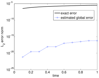
Refer to caption
Fig. 1: Failure to capture the global errors correctly for system y1=1superscriptsubscript𝑦11y_{1}^{\prime}=1, y2=κ2y13superscriptsubscript𝑦2subscript𝜅2superscriptsubscript𝑦13y_{2}^{\prime}=\kappa_{2}y_{1}^{3}, y3=κ3y14superscriptsubscript𝑦3subscript𝜅3superscriptsubscript𝑦14y_{3}^{\prime}=\kappa_{3}y_{1}^{4} solved with RK3(2)G1 (110) [30].

To illustrate this rather subtle point, we consider using the procedure for solving for the correction (30) with method RK3(2)G1 (110) as introduced in [30]. This is a third-order scheme; however, it has no errors that correspond to fourth-order trees and but does not resolve exactly and ; otherwise it would have been a fourth-order method. With the aid of Lemma 6 we construct a simple problem: y1=1superscriptsubscript𝑦11y_{1}^{\prime}=1, y2=κ2y13superscriptsubscript𝑦2subscript𝜅2superscriptsubscript𝑦13y_{2}^{\prime}=\kappa_{2}y_{1}^{3}, y3=κ3y14superscriptsubscript𝑦3subscript𝜅3superscriptsubscript𝑦14y_{3}^{\prime}=\kappa_{3}y_{1}^{4}, where κisubscript𝜅𝑖\kappa_{i} are some constants (e.g., κ2=1/6subscript𝜅216\kappa_{2}=1/6 and κ3=4subscript𝜅34\kappa_{3}=4). For this problem, the RK3(2)G1 is an order 4 method because the tall tree that would have affected the third component is matched exactly by this method. This means that the base method y𝑦y has the same order as the higher-order companion, y^^𝑦\widehat{y}. Therefore, the third component can cause the results to be unreliable. In Fig. 1 we show the third component, which confirms the inadequacy in the error estimation procedure. We note that this analysis also applies to the schemes proposed in [63, 60].

4.4 Second-order explicit Runge-Kutta-like methods

We now introduce a few methods of type [A:GLMGEE] (54). We begin with a detailed inspection of second-order methods. Schemes with s=2𝑠2s=2 are not possible because that would imply that one can have an explicit third-order method by (17) with only two stages, which is a statement that is easy to disprove.

A method with s=3𝑠3s=3 and γ=0𝛾0\gamma=0 in GLyεGLy𝜀{\rm GLy}\varepsilon form is given by the following tableaux,

(65) 𝕄yε=[000101001101/41/40111/121/125/6101/121/121/601],subscript𝕄y𝜀delimited-[]000101001101414011missing-subexpressionmissing-subexpressionmissing-subexpressionmissing-subexpressionmissing-subexpression11211256101121121601\displaystyle{\rm\mathbb{M}_{y\varepsilon}}=\left[\begin{array}[]{ccc|cc}0&0&0&1&0\\ 1&0&0&1&10\\ 1/4&1/4&0&1&-1\\ \hline\cr 1/12&1/12&5/6&1&0\\ 1/12&1/12&-1/6&0&1\\ \end{array}\right]\,,

where the four blocks represent (𝐀yε,𝐔yε,𝐁yε,𝐕yε)subscript𝐀𝑦𝜀subscript𝐔𝑦𝜀subscript𝐁𝑦𝜀subscript𝐕𝑦𝜀(\mathbf{A}_{y\varepsilon},\mathbf{U}_{y\varepsilon},\mathbf{B}_{y\varepsilon},\mathbf{V}_{y\varepsilon}) as discussed above. The diagonal 𝐁𝐔𝐁𝐔\mathbf{B}\mathbf{U} condition is satisfied ([𝐁𝐔]delimited-[]𝐁𝐔[\mathbf{B}\mathbf{U}]); however, the 𝐁𝐀𝐔𝐁𝐀𝐔\mathbf{B}\mathbf{A}\mathbf{U} one is not ([𝐁𝐀𝐔])[\cancel{\mathbf{B}\mathbf{A}\mathbf{U}}]).

Method (65) can then be expressed as follows:

(66a) Y1=subscript𝑌1absent\displaystyle Y_{1}= y[n1],superscript𝑦delimited-[]𝑛1\displaystyle y^{[n-1]}\,,
(66b) Y2=subscript𝑌2absent\displaystyle Y_{2}= y[n1]+10ε[n1]+Δtf(Y1),superscript𝑦delimited-[]𝑛110superscript𝜀delimited-[]𝑛1Δ𝑡𝑓subscript𝑌1\displaystyle y^{[n-1]}+10\varepsilon^{[n-1]}+{\Delta t}f(Y_{1})\,,
(66c) Y3=subscript𝑌3absent\displaystyle Y_{3}= y[n1]ε[n1]+Δt(14f(Y1)+14f(Y2)),superscript𝑦delimited-[]𝑛1superscript𝜀delimited-[]𝑛1Δ𝑡14𝑓subscript𝑌114𝑓subscript𝑌2\displaystyle y^{[n-1]}-\varepsilon^{[n-1]}+{\Delta t}\left(\frac{1}{4}f(Y_{1})+\frac{1}{4}f(Y_{2})\right)\,,
(66d) y[n]=superscript𝑦delimited-[]𝑛absent\displaystyle y^{[n]}= y[n1]+Δt(112f(Y1)+112f(Y2)+56f(Y3)),superscript𝑦delimited-[]𝑛1Δ𝑡112𝑓subscript𝑌1112𝑓subscript𝑌256𝑓subscript𝑌3\displaystyle y^{[n-1]}+{\Delta t}\left(\frac{1}{12}f(Y_{1})+\frac{1}{12}f(Y_{2})+\frac{5}{6}f(Y_{3})\right)\,,
(66e) ε[n]=superscript𝜀delimited-[]𝑛absent\displaystyle\varepsilon^{[n]}= ε[n1]+Δt(112f(Y1)+112f(Y2)16f(Y3)).superscript𝜀delimited-[]𝑛1Δ𝑡112𝑓subscript𝑌1112𝑓subscript𝑌216𝑓subscript𝑌3\displaystyle\varepsilon^{[n-1]}+{\Delta t}\left(\frac{1}{12}f(Y_{1})+\frac{1}{12}f(Y_{2})-\frac{1}{6}f(Y_{3})\right)\,.

In (66) we note the Runge-Kutta structure; however, we see that the defect takes an active role in the stage calculations. Using (53), we obtain the GLyy~GLy~y{\rm GLy\tilde{y}} form as

(72) 𝕄yy~=[000101009101/41/40211/121/125/6101/61/62/301].subscript𝕄y~ydelimited-[]000101009101414021missing-subexpressionmissing-subexpressionmissing-subexpressionmissing-subexpressionmissing-subexpression112112561016162301\displaystyle{\rm\mathbb{M}_{y\tilde{y}}}=\left[\begin{array}[]{ccc|cc}0&0&0&1&0\\ 1&0&0&-9&10\\ 1/4&1/4&0&2&-1\\ \hline\cr 1/12&1/12&5/6&1&0\\ 1/6&1/6&2/3&0&1\\ \end{array}\right]\,.

In particular, (72) is expressed as

(73a) Y1=subscript𝑌1absent\displaystyle Y_{1}= y[n1],superscript𝑦delimited-[]𝑛1\displaystyle y^{[n-1]}\,,
(73b) Y2=subscript𝑌2absent\displaystyle Y_{2}= 9y[n1]+10y~[n1]+Δtf(Y1),9superscript𝑦delimited-[]𝑛110superscript~𝑦delimited-[]𝑛1Δ𝑡𝑓subscript𝑌1\displaystyle-9y^{[n-1]}+10\tilde{y}^{[n-1]}+{\Delta t}f(Y_{1})\,,
(73c) Y3=subscript𝑌3absent\displaystyle Y_{3}= 2y[n1]y~[n1]+Δt(14f(Y1)+14f(Y2)),2superscript𝑦delimited-[]𝑛1superscript~𝑦delimited-[]𝑛1Δ𝑡14𝑓subscript𝑌114𝑓subscript𝑌2\displaystyle 2y^{[n-1]}-\tilde{y}^{[n-1]}+{\Delta t}\left(\frac{1}{4}f(Y_{1})+\frac{1}{4}f(Y_{2})\right)\,,
(73d) y[n]=superscript𝑦delimited-[]𝑛absent\displaystyle y^{[n]}= y[n1]+Δt(112f(Y1)+112f(Y2)+56f(Y3)),superscript𝑦delimited-[]𝑛1Δ𝑡112𝑓subscript𝑌1112𝑓subscript𝑌256𝑓subscript𝑌3\displaystyle y^{[n-1]}+{\Delta t}\left(\frac{1}{12}f(Y_{1})+\frac{1}{12}f(Y_{2})+\frac{5}{6}f(Y_{3})\right)\,,
(73e) y~[n]=superscript~𝑦delimited-[]𝑛absent\displaystyle\tilde{y}^{[n]}= y~[n1]+Δt(16f(Y1)+16f(Y2)+23f(Y3)),ε[n]=y~[n]y[n].superscript~𝑦delimited-[]𝑛1Δ𝑡16𝑓subscript𝑌116𝑓subscript𝑌223𝑓subscript𝑌3superscript𝜀delimited-[]𝑛superscript~𝑦delimited-[]𝑛superscript𝑦delimited-[]𝑛\displaystyle\tilde{y}^{[n-1]}+{\Delta t}\left(\frac{1}{6}f(Y_{1})+\frac{1}{6}f(Y_{2})+\frac{2}{3}f(Y_{3})\right)\,,\quad\varepsilon^{[n]}=\tilde{y}^{[n]}-y^{[n]}\,.

Here we note the explicit contribution of two solutions. A solution of order 3 is obtained according to (17) by y^[n]=y~[n]superscript^𝑦delimited-[]𝑛superscript~𝑦delimited-[]𝑛\widehat{y}^{[n]}=\tilde{y}^{[n]} because γ=0𝛾0\gamma=0. Moreover, a local error estimate for y[n]superscript𝑦delimited-[]𝑛y^{[n]} in (73d) corresponds to

(74) εloc=ε[n]ε[n1]=Δt(112f(Y1)+112f(Y2)16f(Y3)),subscript𝜀locsuperscript𝜀delimited-[]𝑛superscript𝜀delimited-[]𝑛1Δ𝑡112𝑓subscript𝑌1112𝑓subscript𝑌216𝑓subscript𝑌3\displaystyle\varepsilon_{\rm loc}=\varepsilon^{[n]}-\varepsilon^{[n-1]}={\Delta t}\left(\frac{1}{12}f(Y_{1})+\frac{1}{12}f(Y_{2})-\frac{1}{6}f(Y_{3})\right)\,,

which is an obvious statement. This is also obtained by replacing y~[n1]superscript~𝑦delimited-[]𝑛1\tilde{y}^{[n-1]} by y[n]superscript𝑦delimited-[]𝑛y^{[n]} in the right-hand sides of (73) and taking the differences between the two solutions or setting ε[n1]=0superscript𝜀delimited-[]𝑛10\varepsilon^{[n-1]}=0 in (66). Additional second-order methods are given in Appendix A.1. We remark that methods using [A:SolCor] require at least four stages. While this seems like a marginal improvement, it it expected to reap more benefits when considering higher-order methods.

4.5 Third-order explicit Runge-Kutta-like methods

Closed-form solutions were difficult to obtain for methods of order 3. We therefore explored the space of such methods using a numerical optimization such as in [27]. One method of order 3 with γ=0𝛾0\gamma=0, s=5𝑠5s=5 stages, [𝐁𝐔,𝐁𝐀𝐔]𝐁𝐔𝐁𝐀𝐔[\mathbf{B}\mathbf{U},\mathbf{B}\mathbf{A}\mathbf{U}], and having significant negative real axis stability was found to have the following coefficients up to 40 digits accuracy:

(85) a2,1=216960494736370231324313474998937147335,a3,1=4652674649769712389594116917485856474137,a3,2=1029787924402659495849199457603717988219,a4,1=2336478893584598249987425311444725389446,a4,2=79205144337496116638148994349441340815519,a4,3=4005118985931744378236487615018004984309,a5,1=42089522664062539205124911313006412840286,a5,2=15074384760342762939137927286865289746282,a5,3=62274678522253371016125918573676298591413,a5,4=1375547572985247173979257927066651693390,b1,1=6154669683745870372356982519523786160813,b1,2=55810892792806293355206957624151308356511,b1,3=24061048952676379087158739347956038723465,b1,4=35779722068743513397599733370677197135,b1,5=59449832954780563947137360038685338563670,b2,1=973826218698415916899299082461487742983,b2,2=3279709793194861319561521565616362163366,b2,3=4289551460641842063171714201188501437336,b2,4=2260856763316606506855371917805607957003,b2,5=94655809487476459565151517167160302729021,u1,1=7082030913983466155980863923579509469826,u1,2=1004361443967480826780863923579509469826,u2,1=161694774978034105510106187653640211060371,u2,2=55507121337823045139106187653640211060371,u3,1=7848609464456626456888171030896733822981,u3,2=968493625216755841388171030896733822981,u4,1=6539492214633485443584570853840405479554,u4,2=1917593169407062511984570853840405479554,u5,1=8607282770183754108108658046436496925911,u5,2=100050763666313171803108658046436496925911.subscript𝑎21216960494736370231324313474998937147335subscript𝑎314652674649769712389594116917485856474137subscript𝑎321029787924402659495849199457603717988219subscript𝑎412336478893584598249987425311444725389446subscript𝑎4279205144337496116638148994349441340815519subscript𝑎434005118985931744378236487615018004984309subscript𝑎5142089522664062539205124911313006412840286subscript𝑎5215074384760342762939137927286865289746282subscript𝑎5362274678522253371016125918573676298591413subscript𝑎541375547572985247173979257927066651693390subscript𝑏116154669683745870372356982519523786160813subscript𝑏1255810892792806293355206957624151308356511subscript𝑏1324061048952676379087158739347956038723465subscript𝑏1435779722068743513397599733370677197135subscript𝑏1559449832954780563947137360038685338563670subscript𝑏21973826218698415916899299082461487742983subscript𝑏223279709793194861319561521565616362163366subscript𝑏234289551460641842063171714201188501437336subscript𝑏242260856763316606506855371917805607957003subscript𝑏2594655809487476459565151517167160302729021subscript𝑢117082030913983466155980863923579509469826subscript𝑢121004361443967480826780863923579509469826subscript𝑢21161694774978034105510106187653640211060371subscript𝑢2255507121337823045139106187653640211060371subscript𝑢317848609464456626456888171030896733822981subscript𝑢32968493625216755841388171030896733822981subscript𝑢416539492214633485443584570853840405479554subscript𝑢421917593169407062511984570853840405479554subscript𝑢518607282770183754108108658046436496925911subscript𝑢52100050763666313171803108658046436496925911\displaystyle\begin{array}[]{lll}\rule[-7.5pt]{0.0pt}{20.00003pt}a_{2,1}=-\frac{2169604947363702313}{24313474998937147335},&a_{3,1}=\frac{46526746497697123895}{94116917485856474137},&a_{3,2}=-\frac{10297879244026594958}{49199457603717988219},\\ \rule[-7.5pt]{0.0pt}{20.00003pt}a_{4,1}=\frac{23364788935845982499}{87425311444725389446},&a_{4,2}=-\frac{79205144337496116638}{148994349441340815519},&a_{4,3}=\frac{40051189859317443782}{36487615018004984309},\\ \rule[-7.5pt]{0.0pt}{20.00003pt}a_{5,1}=\frac{42089522664062539205}{124911313006412840286},&a_{5,2}=-\frac{15074384760342762939}{137927286865289746282},&a_{5,3}=-\frac{62274678522253371016}{125918573676298591413},\\ \rule[-7.5pt]{0.0pt}{20.00003pt}a_{5,4}=\frac{13755475729852471739}{79257927066651693390},&b_{1,1}=\frac{61546696837458703723}{56982519523786160813},&b_{1,2}=-\frac{55810892792806293355}{206957624151308356511},\\ \rule[-7.5pt]{0.0pt}{20.00003pt}b_{1,3}=\frac{24061048952676379087}{158739347956038723465},&b_{1,4}=\frac{3577972206874351339}{7599733370677197135},&b_{1,5}=-\frac{59449832954780563947}{137360038685338563670},\\ \rule[-7.5pt]{0.0pt}{20.00003pt}b_{2,1}=-\frac{9738262186984159168}{99299082461487742983},&b_{2,2}=-\frac{32797097931948613195}{61521565616362163366},&b_{2,3}=\frac{42895514606418420631}{71714201188501437336},\\ \rule[-7.5pt]{0.0pt}{20.00003pt}b_{2,4}=\frac{22608567633166065068}{55371917805607957003},&b_{2,5}=\frac{94655809487476459565}{151517167160302729021},&u_{1,1}=\frac{70820309139834661559}{80863923579509469826},\\ \rule[-7.5pt]{0.0pt}{20.00003pt}u_{1,2}=\frac{10043614439674808267}{80863923579509469826},&u_{2,1}=\frac{161694774978034105510}{106187653640211060371},&u_{2,2}=-\frac{55507121337823045139}{106187653640211060371},\\ \rule[-7.5pt]{0.0pt}{20.00003pt}u_{3,1}=\frac{78486094644566264568}{88171030896733822981},&u_{3,2}=\frac{9684936252167558413}{88171030896733822981},&u_{4,1}=\frac{65394922146334854435}{84570853840405479554},\\ \rule[-7.5pt]{0.0pt}{20.00003pt}u_{4,2}=\frac{19175931694070625119}{84570853840405479554},&u_{5,1}=\frac{8607282770183754108}{108658046436496925911},&u_{5,2}=\frac{100050763666313171803}{108658046436496925911}.\end{array}

We note that this is not an optimal method. It is just an example that was relatively easy to obtain and will be used in the numerical experiments. We note that method RK3(2)G1 (110) as introduced in [30] requires 8 stages (that number reduces to 7 because of its FSAL property).

5 Relationships with other global error estimation strategies

Here we discuss the relationship between our approach and the existing strategies that we focus on in this study. We show how the latter are particular instantiations of the strategy introduced here. This inclusion is facilitated by the use of Lemma 12, which reveals a linear relationship between propagating two solutions and propagating one solution and its defect. We discuss below in some detail the procedure for solving for the correction and the extrapolation approach. Method [A:ZaPr] follows from the same discussions as those for [A:SolCor]. To express algorithm [A:SoErEq] as a GL method, we need more involved manipulations of these methods. Method [A:ExPrErEq] with the exact principal error equation (21) can obviously be represented as a GL scheme. Methods that implicitly solve the error equation can also be represented as GL schemes; however, in this study we will not expand on this point.

5.1 Approach for solving for the correction

Let us consider the Runge-Kutta methods that integrate the global errors introduced by [30, 33, 31, 63, 60]. The RK tableau is defined by the triplet (𝒜𝒜{\mathcal{A}}, {\mathcal{B}}, 𝒞𝒞{\mathcal{C}}) and the interpolation operators by (Bsuperscript𝐵B^{*}, Dsuperscript𝐷D^{*}), where B[θ0,θ1,,θs]Tsuperscript𝐵superscriptsuperscript𝜃0superscript𝜃1superscript𝜃𝑠𝑇B^{*}\cdot[\theta^{0},\theta^{1},\dots,\theta^{s}]^{T} yields the interpolant weight vector and D[θ0,θ1,,θs]Tsuperscript𝐷superscriptsuperscript𝜃0superscript𝜃1superscript𝜃𝑠𝑇D^{*}\cdot[\theta^{0},\theta^{1},\dots,\theta^{s}]^{T} yields its derivative. In particular, Dij=Bijjsubscriptsuperscript𝐷𝑖𝑗subscriptsuperscript𝐵𝑖𝑗𝑗D^{*}_{ij}=B^{*}_{ij}\cdot j, j=1,,s𝑗1𝑠j=1,\dots,s. Denote by bi(θ)=j=1pBijθjsubscriptsuperscript𝑏𝑖𝜃superscriptsubscript𝑗1superscript𝑝subscriptsuperscript𝐵𝑖𝑗superscript𝜃𝑗b^{*}_{i}(\theta)=\sum_{j=1}^{p^{*}}B^{*}_{ij}\theta^{j}, di(θ)=j=1pDijθjsubscriptsuperscript𝑑𝑖𝜃superscriptsubscript𝑗1superscript𝑝subscriptsuperscript𝐷𝑖𝑗superscript𝜃𝑗d^{*}_{i}(\theta)=\sum_{j=1}^{p^{*}}D^{*}_{ij}\theta^{j}, and consider the dense output formula given by

P(t+θΔt)=yn+θΔti=1sbifiandP(t+θΔt)=θΔti=1sdifi𝑃𝑡𝜃Δ𝑡subscript𝑦𝑛𝜃Δ𝑡superscriptsubscript𝑖1𝑠subscriptsuperscript𝑏𝑖subscript𝑓𝑖andsuperscript𝑃𝑡𝜃Δ𝑡𝜃Δ𝑡superscriptsubscript𝑖1𝑠subscriptsuperscript𝑑𝑖subscript𝑓𝑖\displaystyle P(t+\theta{\Delta t})=y_{n}+\theta{\Delta t}\sum_{i=1}^{s}b^{*}_{i}f_{i}\,~{}\textnormal{and}~{}P^{\prime}(t+\theta{\Delta t})=\theta{\Delta t}\sum_{i=1}^{s}d^{*}_{i}f_{i}\,

and the error equation that is being solved is (30b) (ε(t)=f(t,P(t)+ε(t))P(t)superscript𝜀𝑡𝑓𝑡𝑃𝑡𝜀𝑡superscript𝑃𝑡\varepsilon^{\prime}(t)=f(t,P(t)+\varepsilon(t))-P^{\prime}(t)). We denote by B¯=diag{𝒞}BW(𝒞)Tsuperscript¯𝐵diag𝒞superscript𝐵𝑊superscript𝒞𝑇\overline{B}^{*}=\mathop{\operator@font diag}\nolimits\{{\mathcal{C}}\}\cdot B^{*}\cdot W({\mathcal{C}})^{T}, where W(𝒞)𝑊𝒞W({\mathcal{C}}) is the Vandermonde matrix with entries 𝒞𝒞{\mathcal{C}}; that is, {W(𝒞)}ij=𝒞ij1subscript𝑊𝒞𝑖𝑗superscriptsubscript𝒞𝑖𝑗1\{W({\mathcal{C}})\}_{ij}={\mathcal{C}}_{i}^{j-1}; and D¯=DW(𝒞)Tsuperscript¯𝐷superscript𝐷𝑊superscript𝒞𝑇\overline{D}^{*}=D^{*}\cdot W({\mathcal{C}})^{T}. The resulting method cast in GL format (52) is

(98) [Y1Y2yn+1εn+1]=[𝒜0𝟙s0B¯𝒜D¯𝒜𝟙s𝟙sT010TD¯T01][Δtf(Y1)Δtf(Y2)ynεn].delimited-[]subscript𝑌1subscript𝑌2subscript𝑦𝑛1subscript𝜀𝑛1delimited-[]𝒜0subscript1𝑠0superscript¯𝐵𝒜superscript¯𝐷𝒜subscript1𝑠subscript1𝑠missing-subexpressionmissing-subexpressionmissing-subexpressionmissing-subexpressionsuperscript𝑇010superscript𝑇superscript¯𝐷superscript𝑇01delimited-[]Δ𝑡𝑓subscript𝑌1Δ𝑡𝑓subscript𝑌2subscript𝑦𝑛subscript𝜀𝑛\displaystyle\left[\begin{array}[]{c}Y_{1}\\ Y_{2}\\ y_{n+1}\\ \varepsilon_{n+1}\end{array}\right]=\left[\begin{array}[]{cc|cc}{\mathcal{A}}&0&\mathbbm{1}_{s}&0\\ \overline{B}^{*}-{\mathcal{A}}\overline{D}^{*}&{\mathcal{A}}&\mathbbm{1}_{s}&\mathbbm{1}_{s}\\ \hline\cr{\mathcal{B}}^{T}&0&1&0\\ -{\mathcal{B}}^{T}\overline{D}^{*}&{\mathcal{B}}^{T}&0&1\end{array}\right]\left[\begin{array}[]{c}{\Delta t}f(Y_{1})\\ {\Delta t}f(Y_{2})\\ y_{n}\\ \varepsilon_{n}\end{array}\right]\,.

Here we express the method for a scalar problem, in order to avoid the tensor products, and we represent the stacked stages in Y{1,2}subscript𝑌12Y_{\{1,2\}}. For example, method RK3(2)G1 [30] is given by the following Butcher tableau:

(110) 00121201120116231601623160,B=[13223024303626011]Dij=Bijj.00missing-subexpressionmissing-subexpressionmissing-subexpression12120missing-subexpressionmissing-subexpression1120missing-subexpression11623160missing-subexpressionmissing-subexpressionmissing-subexpressionmissing-subexpressionmissing-subexpression1623160superscript𝐵delimited-[]13223missing-subexpressionmissing-subexpression0243missing-subexpressionmissing-subexpression03626missing-subexpressionmissing-subexpression011missing-subexpressionmissing-subexpressionsubscriptsuperscript𝐷𝑖𝑗subscriptsuperscript𝐵𝑖𝑗𝑗\displaystyle\begin{array}[]{c|cccc}\rule[-7.5pt]{0.0pt}{20.00003pt}0&0\\ \rule[-7.5pt]{0.0pt}{20.00003pt}\frac{1}{2}&\frac{1}{2}&0\\ \rule[-7.5pt]{0.0pt}{20.00003pt}1&-1&2&0\\ \rule[-7.5pt]{0.0pt}{20.00003pt}1&\frac{1}{6}&\frac{2}{3}&\frac{1}{6}&0\\ \cline{1-5}\cr\rule[-7.5pt]{0.0pt}{20.00003pt}&\frac{1}{6}&\frac{2}{3}&\frac{1}{6}&0\end{array}\,,\quad\begin{array}[]{l}B^{*}=\left[\begin{array}[]{ccccc}1&-\frac{3}{2}&\frac{2}{3}\\ 0&2&-\frac{4}{3}\\ 0&\frac{3}{6}&-\frac{2}{6}\\ 0&-1&1\end{array}\right]\\ \rule[-7.5pt]{0.0pt}{20.00003pt}D^{*}_{ij}=B^{*}_{ij}\cdot j\end{array}\,.

The equations to be solved when using the procedure for solving for the correction [A:SolCor] are then (30); however, one can show that they are equivalent to solving (98) and using the strategy [A:GLMGEE] (52) introduced here. The explicit coefficients are listed in tableau (160). This strategy of estimating the global errors is called Runge-Kutta triplets; a similar discussion can be extended for the peer-triplets strategy [84]. The Zadunaisky procedure can be shown to have a similar interpretation; however, it is a little more expensive, and the analysis has to be carried over several steps. We will draw conclusions about its behavior by using [A:SolCor] as a proxy.

5.2 Global error extrapolation

Let us consider again the Runge-Kutta methods defined by the triplet (𝒜𝒜{\mathcal{A}}, {\mathcal{B}}, 𝒞𝒞{\mathcal{C}}) of order p𝑝p. By applying (32) we obtain the method in the GL format,

(126) [Y1Y2Y3yn+1εn+1]=[𝒜00𝟙s0012𝒜0𝟙sβ1𝟙s012T𝟙s12𝒜𝟙sβ1𝟙sT0010βTβ2Tβ2T01][Δtf(Y1)Δtf(Y2)Δtf(Y3)ynεn],delimited-[]subscript𝑌1subscript𝑌2subscript𝑌3subscript𝑦𝑛1subscript𝜀𝑛1delimited-[]𝒜00subscript1𝑠0012𝒜0subscript1𝑠superscript𝛽1subscript1𝑠0tensor-product12superscript𝑇subscript1𝑠12𝒜subscript1𝑠superscript𝛽1subscript1𝑠missing-subexpressionmissing-subexpressionmissing-subexpressionmissing-subexpressionmissing-subexpressionsuperscript𝑇0010𝛽superscript𝑇𝛽2superscript𝑇𝛽2superscript𝑇01delimited-[]Δ𝑡𝑓subscript𝑌1Δ𝑡𝑓subscript𝑌2Δ𝑡𝑓subscript𝑌3subscript𝑦𝑛subscript𝜀𝑛\displaystyle\left[\begin{array}[]{c}Y_{1}\\ Y_{2}\\ \ Y_{3}\\ y_{n+1}\\ \varepsilon_{n+1}\end{array}\right]=\left[\begin{array}[]{ccc|cc}{\mathcal{A}}&0&0&\mathbbm{1}_{s}&0\\ 0&\frac{1}{2}{\mathcal{A}}&0&\mathbbm{1}_{s}&\beta^{-1}\mathbbm{1}_{s}\\ 0&\frac{1}{2}{\mathcal{B}}^{T}\otimes\mathbbm{1}_{s}&\frac{1}{2}{\mathcal{A}}&\mathbbm{1}_{s}&\beta^{-1}\mathbbm{1}_{s}\\ \hline\cr{\mathcal{B}}^{T}&0&0&1&0\\ -\beta{\mathcal{B}}^{T}&\frac{\beta}{2}{\mathcal{B}}^{T}&\frac{\beta}{2}{\mathcal{B}}^{T}&0&1\end{array}\right]\left[\begin{array}[]{c}{\Delta t}f(Y_{1})\\ {\Delta t}f(Y_{2})\\ {\Delta t}f(Y_{3})\\ y_{n}\\ \varepsilon_{n}\end{array}\right]\,,

where β=11γ𝛽11𝛾\beta=\frac{1}{1-\gamma}, γ=1/2p𝛾1superscript2𝑝\gamma=1/2^{p}, and Y{1,2,3}subscript𝑌123Y_{\{1,2,3\}} are the s𝑠s-stage vectors corresponding to the original method stacked on top of each other. This is a method of type (52).

6 Numerical results

In this section we present numerical results with a detailed set of test problems.

6.1 Test problems

We consider a set of simple but comprehensive test problems.

Problem [Prince42] is defined in [67] (4.2) by

(127a) ysuperscript𝑦\displaystyle y^{\prime} =ysin(t)+cos(t),y(0)=κformulae-sequenceabsent𝑦𝑡𝑡𝑦0𝜅\displaystyle=y-\sin(t)+\cos(t)\,,~{}~{}y(0)=\kappa
(127b) y(t)𝑦𝑡\displaystyle y(t) =κexp(t)+sin(t).absent𝜅𝑡𝑡\displaystyle=\kappa*\exp(t)+\sin(t)\,.

Here we take κ=0𝜅0\kappa=0. As a direct consequence of (127b), we see that that any perturbation of the solution y𝑦y, such as numerical errors, leads to exponential growth. Therefore we have an unstable dynamical system; and even if we start with κ=0𝜅0\kappa=0, numerical errors will lead to an exponential solution growth. This is a classical example that is used to show the failure of local error estimation in general and of global error estimation by using Algorithm [A:ExPrErEq] (21) [67] in particular.

A similar problem [Kulikov2013I] is defined by Kulikov [55] by

(128) y1=2ty21/5y4,y2=10texp(5(y31))y4,y3=2ty4,y4=2tln(y1),formulae-sequencesuperscriptsubscript𝑦12𝑡superscriptsubscript𝑦215subscript𝑦4formulae-sequencesuperscriptsubscript𝑦210𝑡5subscript𝑦31subscript𝑦4formulae-sequencesuperscriptsubscript𝑦32𝑡subscript𝑦4superscriptsubscript𝑦42𝑡subscript𝑦1\displaystyle y_{1}^{\prime}=2t\,y_{2}^{1/5}\,y_{4}\,,~{}y_{2}^{\prime}=10t\exp(5(y_{3}-1))\,y_{4}\,,~{}y_{3}^{\prime}=2t\,y_{4}\,,~{}y_{4}^{\prime}=-2t\ln(y_{1})\,,

so that y1(t)=exp(sin(t2))subscript𝑦1𝑡superscript𝑡2y_{1}(t)=\exp(\sin(t^{2})), y2(t)=exp(5sin(t2))subscript𝑦2𝑡5superscript𝑡2y_{2}(t)=\exp(5\sin(t^{2})), y3(t)=sin(t2)+1subscript𝑦3𝑡superscript𝑡21y_{3}(t)=\sin(t^{2})+1, y4(t)=cos(t2)subscript𝑦4𝑡superscript𝑡2y_{4}(t)=\cos(t^{2}). This problem is nonautonomous and exhibits unstable modes later.

To illustrate the error behavior over long time integration, we consider problem [Hull1972B4], which is a nonlinear ODE defined in [50] (B4) by

(129) y1=y2y1y3y12+y22,y2=y1y2y3y12+y22,y3=y1y12+y22,formulae-sequencesuperscriptsubscript𝑦1subscript𝑦2subscript𝑦1subscript𝑦3superscriptsubscript𝑦12superscriptsubscript𝑦22formulae-sequencesuperscriptsubscript𝑦2subscript𝑦1subscript𝑦2subscript𝑦3superscriptsubscript𝑦12superscriptsubscript𝑦22superscriptsubscript𝑦3subscript𝑦1superscriptsubscript𝑦12superscriptsubscript𝑦22\displaystyle y_{1}^{\prime}=-y_{2}-\frac{y_{1}y_{3}}{\sqrt{y_{1}^{2}+y_{2}^{2}}}\,,~{}y_{2}^{\prime}=y_{1}-\frac{y_{2}y_{3}}{\sqrt{y_{1}^{2}+y_{2}^{2}}}\,,~{}y_{3}^{\prime}=\frac{y_{1}}{\sqrt{y_{1}^{2}+y_{2}^{2}}}\,,

with y0=[3,0,0]Tsubscript𝑦0superscript300𝑇y_{0}=[3,0,0]^{T}.

The last problem [LStab2] is used to assess linear stability properties of the proposed numerical methods.

(130c) y=Ay,y(0)=[y1(0),y2(0)]T,A=[abba],Λ(A)={a+ib,aib},formulae-sequencesuperscript𝑦𝐴𝑦formulae-sequence𝑦0superscriptsubscript𝑦10subscript𝑦20𝑇formulae-sequence𝐴delimited-[]𝑎𝑏𝑏𝑎Λ𝐴𝑎𝑖𝑏𝑎𝑖𝑏\displaystyle y^{\prime}=Ay\,,~{}y(0)=[y_{1}(0),y_{2}(0)]^{T}\,,~{}A=\left[\begin{array}[]{cc}a&-b\\ b&a\end{array}\right]\,,~{}\Lambda(A)=\{a+ib,a-ib\}\,,
(130f) {y1(t)=exp(at)(y2(0)cos(bt)y1(0)sin(bt))y2(t)=exp(at)(y1(0)cos(bt)+y2(0)sin(bt)).casessubscript𝑦1𝑡𝑎𝑡subscript𝑦20𝑏𝑡subscript𝑦10𝑏𝑡subscript𝑦2𝑡𝑎𝑡subscript𝑦10𝑏𝑡subscript𝑦20𝑏𝑡\displaystyle\left\{\begin{array}[]{l}y_{1}(t)=\exp(at)\left(y_{2}(0)\cos(bt)-y_{1}(0)\sin(bt)\right)\\ y_{2}(t)=\exp(at)\left(y_{1}(0)\cos(bt)+y_{2}(0)\sin(bt)\right)\end{array}\right.\,.

This problem allows one to choose the position of the eigenvalues of the Jacobian, Λ(A)Λ𝐴\Lambda(A), in order to simulate problems with different spectral properties.

6.2 Numerical experiments

We begin with simple numerical experiments that show when local error control without global error estimates is not suitable. We therefore compare the result of well-tuned numerical integrators that use local error control with the global error estimates for the same problem. We use Matlab’s ode45 integrator with different tolerances whenever we refer to methods with local error estimation.

In Fig. 2 we show the errors over time for problems [Prince42] (127) and [Kulikov2013I] (128). These problems are solved by using LEE methods, Figs. 2(a)-2(b), and GEE methods, (136) and (149), Figs. 2(c)-2(d); furthermore, the other GEE methods introduced above give similar results. The absolute error tolerance for LEE control is set to 1e-02. The methods with LEE systematically underestimate the global error levels as expected, whereas the methods with GEE capture the errors relatively well. Moreover, the global errors are captured well across components, as shown in Fig. 2(d). The LEE results are intended to show unreliability in accuracy; however, this setting is not suitable for comparing efficiency between LEE and GEE because LEE methods are not designed to account for or estimate the global error. The point of GEE methods is that they provide global error estimates whereas LEE methods do not; however, in this case the GEE methods do not perform step-size adaptivity to improve efficiency, as is done with the LEE methods.
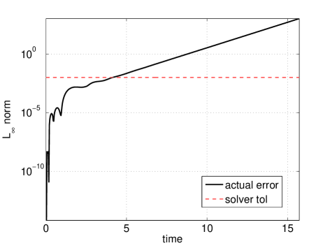
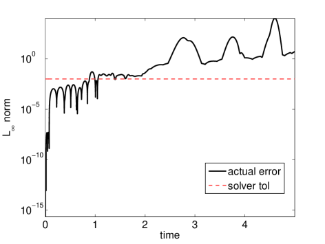
Refer to caption
(a) [Prince42] (127) with LEE
Refer to caption
(b) [Kulikov2013I] (128) with LEE
Refer to caption
(c) Problem (a) with GEE
Refer to caption
(d) Problem (b) with GEE, by components
Fig. 2: Errors when solving problems with unstable modes by using local estimated error (LEE) control and global error estimation (GEE). The absolute error tolerance for LEE control is set to 1e-02. The GEE method used here is (136) with Δt=3e02Δ𝑡3𝑒02{\Delta t}=3e-02 in (c) and (149) with Δt=5e04Δ𝑡5𝑒04{\Delta t}=5e-04 in (d). GEE captures the errors well, whereas LEE underestimates them severely.

In Fig. 3 we show the error behavior for problem [Hull1972B4] (129) when long integration windows are considered. For LEE we set the absolute tolerance to 1e-05. In this case we observe an error drift to levels of 1e-03 over 1,000 time units. The method with GEE (149) can follow closely the error in time. We note that methods (65) and (136) with [𝐁𝐀𝐔]delimited-[]cancel𝐁𝐀𝐔[\cancel{\mathbf{B}\mathbf{A}\mathbf{U}}] do not perform well. Therefore, the built-in error estimator in the GEE method to maintain its accuracy over time, we need to decouple the two embedded schemes further by ensuring that 𝐁𝐀𝐔𝐁𝐀𝐔\mathbf{B}\mathbf{A}\mathbf{U} is a diagonal matrix; moreover, both GEE methods that satisfy this property perform well on this test case. This aspect is observed for all methods introduced here, discussed further below, and illustrated in Fig. 6.

Refer to caption
(a) LEE for (129)
Refer to caption
(b) LEE for long times
Refer to caption
(c) GEE for long times
Fig. 3: Errors when solving [Hull1972B4] (129) with LEE and GEE. For LEE we set the absolute tolerance to 1e-05. (a) During short integration times LEE satisfies the error tolerance well. (b) For longer times, however, we see an expected drift to error levels of 1e-03. (c) GEE method with Δt=0.005Δ𝑡0.005{\Delta t}=0.005 and diagonal 𝐁𝐀𝐔𝐁𝐀𝐔\mathbf{B}\mathbf{A}\mathbf{U} (149) gives accurate error estimates even over long times, while GEE with non-diagonal 𝐁𝐀𝐔𝐁𝐀𝐔\mathbf{B}\mathbf{A}\mathbf{U} (65) and (136) do not.
Convergence analysis

We next analyze the convergence properties of the methods discussed here. In Fig. 4 we show the convergence of the solution and of the error estimate. Here we illustrate the convergence of GEE methods of orders 2 (142) and 3 (85) for problem [Prince42] (127). All GEE methods introduced in this study converge with their prescribed order; moreover, the error estimate also converges with order p+1𝑝1p+1, as expected from (17). In Fig. 5 we show the behavior of global error estimation when using methods satisfying the exact principal error equation. Here we use method [67, (3.11)], which fails to capture the error magnitude as discussed in [67] because the estimated error is several orders of magnitude smaller than the true global error.
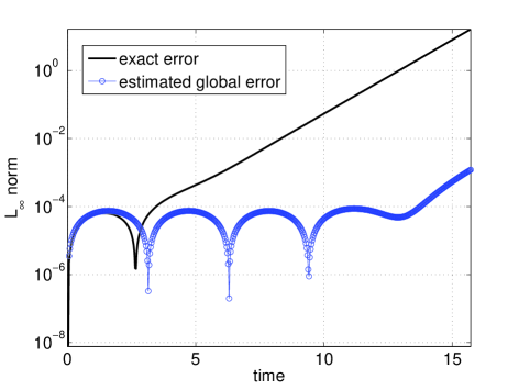
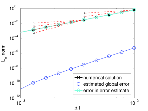
Refer to caption
(a) Second-order method (142)
Refer to caption
(b) Third-order method (85)
Fig. 4: Convergence of GEE methods for problem [Prince42] (127). In (a) we show the error in the solution obtained by the second-order GEE method (142) and the estimated global error, which follows it closely, as well as the difference between the true error and the error estimate. An asymptotic guide is provided by the red dashed lines. (b) This is the same as (a) but using the third-order method (85).
Refer to caption
(a) Error estimation for methods with exact principal error equation for problem [Prince42]
Refer to caption
(b) Method [67, (3.11)]
Fig. 5: (a) Failure to capture the global errors correctly for problem [Prince42] (127) when using a method with exact error equation such as [67, (3.11)] with Δt=3e02Δ𝑡3𝑒02{\Delta t}=3e-02 and (b) its convergence analysis.

In Fig. 6 we illustrate the effect of having different coupling conditions satisfied. In particular, if 𝐁𝐔𝐁𝐔\mathbf{B}\mathbf{U} is not diagonal, the GEE may not converge at all (see Fig. 6(a)). This method is obtained by replacing the first row of 𝐁yy~subscript𝐁𝑦~𝑦\mathbf{B}_{y\tilde{y}} by [0,0,1] and 𝐔yy~=[413/4501/4]Tsubscript𝐔𝑦~𝑦superscriptmatrix41345014𝑇\mathbf{U}_{y\tilde{y}}=\scriptsize{\begin{bmatrix}-4&1&3/4\\ 5&0&1/4\end{bmatrix}}^{T} in (72). If 𝐁𝐔𝐁𝐔\mathbf{B}\mathbf{U} is diagonal but 𝐁𝐀𝐔𝐁𝐀𝐔\mathbf{B}\mathbf{A}\mathbf{U} is not, the method may converge more slowly to the asymptotic regime as the high-order error coupling terms become negligible (see Fig. 6(b)). In Fig. 6(c), we show the convergence for the same problem when both 𝐁𝐔𝐁𝐔\mathbf{B}\mathbf{U} and 𝐁𝐀𝐔𝐁𝐀𝐔\mathbf{B}\mathbf{A}\mathbf{U} are diagonal.

Refer to caption
(a) similar to (72), 𝐁𝐔cancel𝐁𝐔\cancel{\mathbf{B}\mathbf{U}}, 𝐁𝐀𝐔cancel𝐁𝐀𝐔\cancel{\mathbf{B}\mathbf{A}\mathbf{U}}
Refer to caption
(b) (136), 𝐁𝐔𝐁𝐔\mathbf{B}\mathbf{U}, 𝐁𝐀𝐔cancel𝐁𝐀𝐔\cancel{\mathbf{B}\mathbf{A}\mathbf{U}}
Refer to caption
(c) (149), 𝐁𝐔𝐁𝐔\mathbf{B}\mathbf{U}, 𝐁𝐀𝐔𝐁𝐀𝐔\mathbf{B}\mathbf{A}\mathbf{U}
Fig. 6: Convergence of second-order GEE methods with different decoupling properties for [Kulikov2013I]. (a) Not satisfying 𝐁𝐔𝐁𝐔\mathbf{B}\mathbf{U} leads to a lack of convergence. (b) Satisfying just 𝐁𝐔𝐁𝐔\mathbf{B}\mathbf{U} but not 𝐁𝐀𝐔𝐁𝐀𝐔\mathbf{B}\mathbf{A}\mathbf{U} may lead to slower convergence. (c) Satisfying both 𝐁𝐔𝐁𝐔\mathbf{B}\mathbf{U} or 𝐁𝐀𝐔𝐁𝐀𝐔\mathbf{B}\mathbf{A}\mathbf{U} leads to consistent convergence properties.
Linear stability

We next look at the linear stability properties of the methods introduced in this study. In Fig. 7(a) we delineate the stability regions according to (47). In Fig. 7(b) we show numerical results for problem [LStab2] (130) with λΔt={14,12,34,1}×(1±1)𝜆Δ𝑡1412341plus-or-minus11\lambda{\Delta t}=\{\frac{1}{4},\frac{1}{2},\frac{3}{4},1\}\times(-1\pm\sqrt{-1}) when using method (136). As expected, all solutions except the one corresponding to λΔt=1±1𝜆Δ𝑡plus-or-minus11\lambda{\Delta t}=-1\pm\sqrt{-1} are stable, as can be interpreted from Fig. 7(a).

Refer to caption
(a) Stability regions for second-order methods (73), (136), (142), and third-order (85)
Refer to caption
(b) Solution of [LStab2] (130) when using method (136)
Fig. 7: Linear stability regions for four methods introduced in this study (a); and the solution of method (136) for problem [LStab2] (130) in (b) with different time steps. Spectral radius of (136) is indicated in (a) with marker * of the same color. Solutions in (b) are stable except the one (cyan line) for which the eigenvalues are outside the corresponding stability region (red line) in (a).
Adaptive time stepping and practical considerations

Two practical situations are illustrated next: (i)𝑖(i) a situation in which local error control is used to adapt the time steps and the global error estimate is used to validate the solution accuracy and (ii)𝑖𝑖(ii) a situation in which a prescribed level of accuracy is needed, which requires recomputing the solution with a different time step. In the first case we consider a simple local error control using local error estimates (54b) provided by GEE (85). The local error control is achieved by using standard approaches [43, II.4]. In Fig. 8 we show the error evolution [Kulikov2013I] while attempting to restrict the local error to be around 1e-05. The time-step length is allowed to vary between 1e-03 and 1e-05. Note that the global error estimate remains faithful under the time-step change as expected based on the discussion at the end of Sec. 2 following (18). We also show that summing the local errors via cumulative sum (cumsum) yields precisely the global error as suggested by (54b). Similar conditions are used in the second case in which the target is to satisfy a prescribed tolerance. In a first run the time step is fixed to 0.0001, and an integration is carried out to the final time. The global error and the asymptotic are used to determine the time step that would guarantee a global error of 1e-04. A simple asymptotic analysis indicates that a time step of 0.00013 needs to be used in order to achieve that target for GEE (85). The solution is recomputed by using this smaller fixed time-step, and the global errors shown in Fig. 9 satisfy the prescribed global accuracy. We note that this case is just an illustration of the theoretical properties of the methods introduced here. It is likely a suboptimal strategy for achieving a prescribed global tolerance.
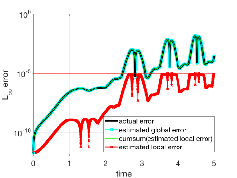
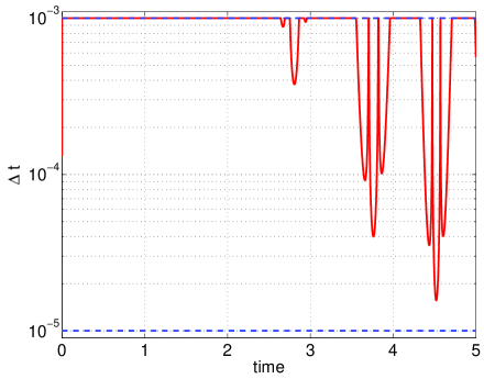
Refer to caption
Refer to caption
Fig. 8: Time-step adaptivity using a local error controller. The GEE method (85) is used to integrate problem [Kulikov2013I] by restricting local error to be less than 1e-05. The error evolution is shown on the left, and the time-step length is shown on the right panel. The time-step length is allowed to vary between 1e-03 and 1e-05.
Refer to caption
Refer to caption
Fig. 9: Error evolution for [Kulikov2013I] when using the GEE method (85) with Δt=0.001Δ𝑡0.001{\Delta t}=0.001 (left) and Δt=0.00013Δ𝑡0.00013{\Delta t}=0.00013 (right). The smaller time step has been calculated based on the GEE global error estimate to keep the global errors below 1e-04.

7 Discussion

In this study we introduce a new strategy for global error estimation in time-stepping methods. This strategy is based on advancing in time the solution along with the defect or, equivalently, two solutions that have a fixed relation between their truncation errors. The main idea is summarized in Theorem 9, and practical considerations are brought up by Proposition 14. This translates in a particular relation among the truncation errors of GL outputs and in a decoupling constraint. We note that this strategy can be seen as a generalization of the procedure for solving for the correction and of several others from the same class. We provide equivalent representation of these methods in the proposed GL form (52).

We have explored several algorithms in this study. The methods [A:ExPrErEq] with exact principal error equation (21) [80] are attractive because they offer global error estimates extremely cheaply; however, they were shown in [67] to be unreliable as illustrated in Fig. 5. Strategies that directly solve the error equation, such as [A:SoErEq] (28), need a reliable way of estimating the local errors and the availability of the Jacobian. We found these methods to be robust, especially the strategy proposed in [58] for low-order methods. The procedure for solving for the correction [A:SolCor] (30) is arguably one of the most popular approaches for global error estimation. It is related to [A:ZaPr] and [A:SoErEq], as discussed, and a particular case of this approach is introduced in this study. The extrapolation algorithm [A:Ex] (33) is the most robust; however, it is also the most expensive and also a particular case of [A:GLMGEE]. With respect to global error control, Kulikov and Weiner [55, 84] report very promising results.

The methods introduced here are based on a general linear representation. The particular case under study is given by form (52); however, the analysis is not restricted to that situation. Particular instances of second and third order are presented throughout this study. The error estimates can be used for error control; however, in this study we do not address this issue. The GL representation allows stages to be reused or shared among the solutions that are propagated within. This leads to methods having lower costs. Moreover, the stability analysis is simplified when compared with global error strategies that use multiple formulas or equations. We consider only GL methods with two solutions, but this concept can be extended to having multiple values propagated in time (e.g., multistep-multistage or peer methods).

We provide several numerical experiments in which we illustrate the behavior of the global error estimation procedures introduced here, their convergence behavior, and their stability properties.

We investigate nonstiff differential equations. Additional constraints are necessary in order to preserve error estimation and avoid order reduction necessary for stiff ODEs.

Global error estimation is typically not used in practice because of its computational expense. This study targets strategies that would make it cheaper to estimate the global errors and therefore make them more practical.

Appendix A Second-order methods

A.1 Other GL second-order methods

Here we provide two additional second-order methods that we used in our experiments. A second-order method with s=3𝑠3s=3, [𝐁𝐔,𝐁𝐀𝐔]𝐁𝐔cancel𝐁𝐀𝐔[\mathbf{B}\mathbf{U},\cancel{\mathbf{B}\mathbf{A}\mathbf{U}}], and γ=0𝛾0\gamma=0 in GLyεGLy𝜀{\rm GLy}\varepsilon format is given by

(136) 𝕄yε=[00014100104/92/901001/23/2101/41/23/401].subscript𝕄y𝜀delimited-[]00014100104929010missing-subexpressionmissing-subexpressionmissing-subexpressionmissing-subexpressionmissing-subexpression012321014123401\displaystyle{\rm\mathbb{M}_{y\varepsilon}}=\left[\begin{array}[]{ccc|cc}0&0&0&1&4\\ 1&0&0&1&0\\ 4/9&2/9&0&1&0\\ \hline\cr 0&-1/2&3/2&1&0\\ 1/4&1/2&-3/4&0&1\\ \end{array}\right]\,.

Another second-order method with s=3𝑠3s=3 and [𝐁𝐔,𝐁𝐀𝐔]𝐁𝐔cancel𝐁𝐀𝐔[\mathbf{B}\mathbf{U},\cancel{\mathbf{B}\mathbf{A}\mathbf{U}}] that is based on two second-order approximations (γ=1/2𝛾12\gamma=1/2) in GLyεGLy𝜀{\rm GLy}\varepsilon format is given by

(142) 𝕄yε=[000111/10100113/304/92/9015/35/125/121/6101/41/41/201].subscript𝕄y𝜀delimited-[]000111101001133049290153missing-subexpressionmissing-subexpressionmissing-subexpressionmissing-subexpressionmissing-subexpression512512161014141201\displaystyle{\rm\mathbb{M}_{y\varepsilon}}=\left[\begin{array}[]{ccc|cc}0&0&0&1&-11/10\\ 1&0&0&1&13/30\\ 4/9&2/9&0&1&5/3\\ \hline\cr 5/12&5/12&1/6&1&0\\ -1/4&-1/4&1/2&0&1\\ \end{array}\right]\,.

A second order method that results in having both 𝐁𝐔𝐁𝐔\mathbf{B}\mathbf{U} and 𝐁𝐀𝐔𝐁𝐀𝐔\mathbf{B}\mathbf{A}\mathbf{U} diagonal matrices is a four-stage method with the following coefficients in GLyy~GLy~y{\rm GLy\tilde{y}} form:

(149) 𝐀2,1=3/4,𝐀3,1=1/4,𝐀3,2=29/60,𝐀4,1=21/44,𝐀4,2=145/44,𝐀4,3=20/11,𝐁1,1=109/275,𝐁1,2=58/75,𝐁1,3=37/110,𝐁1,4=1/6,𝐁2,1=3/11,𝐁2,3=75/88,𝐁2,4=1/8,𝐔2,1=75/58,𝐔1,2=1,𝐔2,2=17/58,𝐔3,2=1,𝐔4,2=1,subscript𝐀2134subscript𝐀3114subscript𝐀322960missing-subexpressionsubscript𝐀412144subscript𝐀4214544subscript𝐀432011missing-subexpressionsubscript𝐁11109275subscript𝐁125875subscript𝐁1337110subscript𝐁1416subscript𝐁21311missing-subexpressionsubscript𝐁237588subscript𝐁2418missing-subexpressionsubscript𝐔217558missing-subexpressionmissing-subexpressionsubscript𝐔121subscript𝐔221758subscript𝐔321subscript𝐔421\displaystyle\begin{array}[]{llll}\mathbf{A}_{2,1}=3/4,&\mathbf{A}_{3,1}=1/4,&\mathbf{A}_{3,2}=29/60,\\ \mathbf{A}_{4,1}=-21/44,&\mathbf{A}_{4,2}=145/44,&\mathbf{A}_{4,3}=-20/11,\\ \mathbf{B}_{1,1}=109/275,&\mathbf{B}_{1,2}=58/75,&\mathbf{B}_{1,3}=-37/110,&\mathbf{B}_{1,4}=1/6,\\ \mathbf{B}_{2,1}=3/11,&&\mathbf{B}_{2,3}=75/88,&\mathbf{B}_{2,4}=-1/8,\\ &\mathbf{U}_{2,1}=75/58,&\\ \mathbf{U}_{1,2}=1,&\mathbf{U}_{2,2}=-17/58,&\mathbf{U}_{3,2}=1,&\mathbf{U}_{4,2}=1,\end{array}

where the rest of the coefficients are zero.

Appendix B RK3(2)G1 [30] in GL form (52)

Method (98) corresponding to RK3(2)G1 (110) [30] results in the following tableau in GLyεGLy𝜀{\rm GLy}\varepsilon form:

(160) 𝕄yε=[00000000101/200000001012000000101/62/31/6000001000000000117/241/31/121/81/2000117/64/31/31/212001100001/62/31/60111/62/31/600000101/62/31/601/62/31/6001].subscript𝕄y𝜀delimited-[]00000000101200000001012000000101623160000010000000001172413112181200011764313121200110000162316011missing-subexpressionmissing-subexpressionmissing-subexpressionmissing-subexpressionmissing-subexpressionmissing-subexpressionmissing-subexpressionmissing-subexpressionmissing-subexpressionmissing-subexpression16231600000101623160162316001\displaystyle{\rm\mathbb{M}_{y\varepsilon}}=\left[\begin{array}[]{cccccccc|cc}0&0&0&0&0&0&0&0&1&0\\ 1/2&0&0&0&0&0&0&0&1&0\\ -1&2&0&0&0&0&0&0&1&0\\ 1/6&2/3&1/6&0&0&0&0&0&1&0\\ 0&0&0&0&0&0&0&0&1&1\\ -7/24&1/3&1/12&-1/8&1/2&0&0&0&1&1\\ 7/6&-4/3&-1/3&1/2&-1&2&0&0&1&1\\ 0&0&0&0&1/6&2/3&1/6&0&1&1\\ \hline\cr 1/6&2/3&1/6&0&0&0&0&0&1&0\\ -1/6&-2/3&-1/6&0&1/6&2/3&1/6&0&0&1\\ \end{array}\right]\,.

Appendix C Second-order method with exact principal error equation

The following method is of type (21) and introduced in [67, (3.11)]:

(173) 𝕊:=001212058058013012815,𝕄:=0012120341214023143,𝔽:=00121203412140294231422221.formulae-sequenceassign𝕊00missing-subexpressionmissing-subexpression12120missing-subexpression580580missing-subexpressionmissing-subexpressionmissing-subexpressionmissing-subexpression13012815formulae-sequenceassign𝕄00missing-subexpressionmissing-subexpression12120missing-subexpression3412140missing-subexpressionmissing-subexpressionmissing-subexpressionmissing-subexpression23143assign𝔽00missing-subexpressionmissing-subexpression12120missing-subexpression3412140missing-subexpressionmissing-subexpressionmissing-subexpressionmissing-subexpression294231422221\displaystyle\mathbb{S}:=\begin{array}[]{c|ccc}\rule[-7.5pt]{0.0pt}{20.00003pt}0&0\\ \rule[-7.5pt]{0.0pt}{20.00003pt}\frac{1}{2}&\frac{1}{2}&0\\ \rule[-7.5pt]{0.0pt}{20.00003pt}\frac{5}{8}&0&\frac{5}{8}&0\\ \cline{1-4}\cr\rule[-7.5pt]{0.0pt}{20.00003pt}&-\frac{1}{30}&\frac{1}{2}&\frac{8}{15}\end{array}\,,~{}~{}\mathbb{M}:=\begin{array}[]{c|ccc}\rule[-7.5pt]{0.0pt}{20.00003pt}0&0\\ \rule[-7.5pt]{0.0pt}{20.00003pt}\frac{1}{2}&\frac{1}{2}&0\\ \rule[-7.5pt]{0.0pt}{20.00003pt}\frac{3}{4}&\frac{1}{2}&\frac{1}{4}&0\\ \cline{1-4}\cr\rule[-7.5pt]{0.0pt}{20.00003pt}&\frac{2}{3}&-1&\frac{4}{3}\end{array}\,,~{}~{}\mathbb{F}:=\begin{array}[]{c|ccc}\rule[-7.5pt]{0.0pt}{20.00003pt}0&0\\ \rule[-7.5pt]{0.0pt}{20.00003pt}\frac{1}{2}&\frac{1}{2}&0\\ \rule[-7.5pt]{0.0pt}{20.00003pt}\frac{3}{4}&\frac{1}{2}&\frac{1}{4}&0\\ \cline{1-4}\cr\rule[-7.5pt]{0.0pt}{20.00003pt}&-\frac{29}{42}&-\frac{31}{42}&\frac{22}{21}\end{array}\,.

References

  • [1] R. Aïd and L. Levacher, Numerical investigations on global error estimation for ordinary differential equations, Journal of Computational and Applied Mathematics, 82 (1997), pp. 21–39.
  • [2] S. Balay, S. Abhyankar, M.F. Adams, J. Brown, P. Brune, K. Buschelman, V. Eijkhout, W.D. Gropp, D. Kaushik, M.G. Knepley, L.C. McInnes, K. Rupp, B.F. Smith, and H. Zhang, PETSc users manual, Tech. Report ANL-95/11 - Revision 3.5, Argonne National Laboratory, 2014.
  • [3] J.W. Banks, J.A.F. Hittinger, J.M. Connors, and C.S. Woodward, Numerical error estimation for nonlinear hyperbolic PDEs via nonlinear error transport, Computer Methods in Applied Mechanics and Engineering, 213–216 (2012), pp. 1–15.
  • [4] M. Berzins, Global error estimation in the method of lines for parabolic equations, SIAM Journal on Scientific and Statistical Computing, 9 (1988), pp. 687–703.
  • [5] K. Burrage and J.C. Butcher, Non-linear stability of a general class of differential equation methods, BIT, 20 (1980), pp. 185–203.
  • [6] J.C. Butcher, Coefficients for the study of Runge-Kutta integration processes, Journal of the Australian Mathematical Society, 3 (1963), pp. 185–201.
  • [7] J.C. Butcher, A modified multistep method for the numerical integration of ordinary differential equations, J. ACM, 12 (1965), pp. 124–135.
  • [8]  , On the convergence of numerical solutions to ordinary differential equations, Mathematics of Computation, 20 (1966), pp. 1–10.
  • [9] J.C. Butcher, The effective order of Runge-Kutta methods, in Conference on the numerical solution of differential equations, Springer, 1969, pp. 133–139.
  • [10] J.C. Butcher, An algebraic theory of integration methods, Mathematics of Computation, 26 (1972), pp. 79–106.
  • [11] J.C. Butcher, Order and effective order, Applied Numerical Mathematics, 28 (1998), pp. 179–191.
  • [12] J.C. Butcher, General linear methods for stiff differential equations, BIT, 41 (2001), pp. 240–264.
  • [13] J.C. Butcher, The A-stability of methods with Padé and generalized Padé stability functions, Numerical Algorithms, 31 (2002), pp. 47–58.
  • [14] J.C. Butcher, General linear methods, Acta Numerica, 15 (2006), pp. 157–256.
  • [15]  , Numerical Methods for Ordinary Differential Equations, Wiley, second ed., 2008.
  • [16] J.C. Butcher and P. Chartier, A generalization of singly-implicit Runge-Kutta methods, Applied Numerical Mathematics, 24 (1997), pp. 343–350.
  • [17]  , The effective order of singly-implicit Runge-Kutta methods, Numerical Algorithms, 20 (1999), pp. 269–284.
  • [18] J.C. Butcher and D.J.L. Chen, ESIRK methods and variable stepsize, Applied Numerical Mathematics, 28 (1998), pp. 193–207.
  • [19] J.C. Butcher and M.T. Diamantakis, DESIRE: Diagonally extended singly implicit Runge–Kutta effective order methods, Numerical Algorithms, 17 (1998), pp. 121–145.
  • [20] J.C. Butcher and Z. Jackiewicz, A new approach to error estimation for general linear methods, Numerische Mathematik, 95 (2003), pp. 487–502.
  • [21] Y. Cao and L. Petzold, A posteriori error estimation and global error control for ordinary differential equations by the adjoint method, SIAM Journal on Scientific Computing, 26 (2005), pp. 359–374.
  • [22] J.R. Cash and A.H. Karp, A variable order Runge-Kutta method for initial value problems with rapidly varying right-hand sides, ACM Transactions on Mathematical Software (TOMS), 16 (1990), pp. 201–222.
  • [23] J.-C. Chang, T.M.H. Chan, and D.J.L. Chen, Enhanced order composition methods, Applied Numerical Mathematics, 58 (2008), pp. 223–235.
  • [24] P. Chartier, E. Hairer, and G. Vilmart, Algebraic structures of B-series, Foundations of Computational Mathematics, 10 (2010), pp. 407–427.
  • [25] J. Connors, J. Banks, J. Hittinger, and C. Woodward, A method to calculate numerical errors using adjoint error estimation for linear advection, SIAM Journal on Numerical Analysis, 51 (2013), pp. 894–926.
  • [26] E.M. Constantinescu, On the order of general linear methods, Applied Mathematics Letters, 22 (2009), pp. 1425–1428.
  • [27] E.M. Constantinescu and A. Sandu, Optimal explicit strong-stability-preserving general linear methods, SIAM Journal on Scientific Computing, 32 (2010), pp. 3130–3150.
  • [28] G.J. Cooper, The order of convergence of general linear methods for ordinary differential equations, SIAM Journal on Numerical Analysis, 15 (1978), pp. 643–661.
  • [29] Germund Dahlquist, On the control of the global error in stiff initial value problems, in Numerical Analysis, G. Watson, ed., vol. 912 of Lecture Notes in Mathematics, Springer Berlin Heidelberg, 1982, pp. 38–49. 10.1007/BFb0093147.
  • [30] J.R. Dormand, R.R. Duckers, and P.J. Prince, Global error estimation with Runge-Kutta methods, IMA Journal of Numerical Analysis, 4 (1984), pp. 169–184.
  • [31] J.R. Dormand, J.P. Gilmore, and P.J. Prince, Globally embedded Runge-Kutta schemes, Ann. Numer. Math, 1 (1994), pp. 97–106.
  • [32] J.R. Dormand, M.A. Lockyer, N.E. McGorrigan, and P.J. Prince, Global error estimation with Runge-Kutta triples, Computers & Mathematics with Applications, 18 (1989), pp. 835–846.
  • [33] J.R. Dormand and P.J. Prince, Global error estimation with Runge-Kutta methods II, IMA Journal of Numerical Analysis, 5 (1985), pp. 481–497.
  • [34] W.H. Enright, Analysis of error control strategies for continuous Runge-Kutta methods, SIAM Journal on Numerical Analysis, 26 (1989), pp. 588–599.
  • [35]  , Continuous numerical methods for ODEs with defect control, Journal of Computational and Applied Mathematics, 125 (2000), pp. 159–170.
  • [36] D. Estep, A posteriori error bounds and global error control for approximation of ordinary differential equations, SIAM Journal on Numerical Analysis, 32 (1995), pp. 1–48.
  • [37] D. Estep, M. Holst, and M. Larson, Generalized Green’s functions and the effective domain of influence, SIAM Journal on Scientific Computing, 26 (2005), pp. 1314–1339.
  • [38] C.W. Gear, Hybrid methods for initial value problems in ordinary differential equations, SIAM Journal on Numerical Analysis, 2 (1965), pp. 69–86.
  • [39] Michael B Giles and Endre Süli, Adjoint methods for PDEs: A posteriori error analysis and postprocessing by duality, Acta Numerica, 11 (2002), pp. 145–236.
  • [40] W.B. Gragg and H.J. Stetter, Generalized multistep predictor-corrector methods, JACM, 11 (1964), pp. 188–209.
  • [41] Y. Hadjimichael, C. Macdonald, D. Ketcheson, and J. Verner, Strong stability preserving explicit Runge–Kutta methods of maximal effective order, SIAM Journal on Numerical Analysis, 51 (2013), pp. 2149–2165.
  • [42] E. Hairer and C. Lubich, Asymptotic expansions of the global error of fixed-stepsize methods, Numerische Mathematik, 45 (1984), pp. 345–360.
  • [43] E. Hairer, S.P. Nørsett, and G. Wanner, Solving Ordinary Differential Equations I: Nonstiff Problems, Springer, 2008.
  • [44] E. Hairer and G. Wanner, Multistep-multistage-multiderivative methods for ordinary differential equations, Computing, 11 (1973), pp. 287–303.
  • [45]  , On the Butcher group and general multi-value methods, Computing, 13 (1974), pp. 1–15.
  • [46] P. Henrici, Discrete Variable Methods in Ordinary Differential Equations, New York: Wiley, 1962, 1962.
  • [47] M. Heroux, R. Bartlett, V.H.R. Hoekstra, J. Hu, T. Kolda, R. Lehoucq, K. Long, R. Pawlowski, E. Phipps, A. Salinger, H. Thornquist, R. Tuminaro, J. Willenbring, and A. Williams, An overview of Trilinos, Tech. Report SAND2003-2927, Sandia National Laboratories, 2003.
  • [48] D.J. Higham, Global error versus tolerance for explicit Runge-Kutta methods, IMA Journal of Numerical Analysis, 11 (1991), pp. 457–480.
  • [49] A.C. Hindmarsh, P.N. Brown, K.E. Grant, S.L. Lee, R. Serban, D.E. Shumaker, and C.S. Woodward, SUNDIALS: Suite of nonlinear and differential/algebraic equation solvers, ACM Transactions on Mathematical Software (TOMS), 31 (2005), pp. 363–396.
  • [50] T.E. Hull, W.H. Enright, B.M. Fellen, and A.E. Sedgwick, Comparing numerical methods for ordinary differential equations, SIAM Journal on Numerical Analysis, 9 (1972), pp. 603–637.
  • [51] Z. Jackiewicz, General Linear Methods for Ordinary Differential Equations, Wiley-Interscience, John Wiley & Sons, 2009.
  • [52] C.P. Jeannerod and J. Visconti, Global error estimation for index-1 and -2 DAEs, Numerical Algorithms, 19 (1998), pp. 111–125.
  • [53] G.Y. Kulikov, On quasi-consistent integration by Nordsieck methods, Journal of Computational and Applied Mathematics, 225 (2009), pp. 268–287.
  • [54]  , Global error control in adaptive Nordsieck methods, SIAM Journal on Scientific Computing, 34 (2012), pp. A839–A860.
  • [55]  , Cheap global error estimation in some Runge-Kutta pairs, IMA Journal of Numerical Analysis, 33 (2013), pp. 136–163.
  • [56] G.Y. Kulikov and R. Weiner, Doubly quasi-consistent parallel explicit peer methods with built-in global error estimation, Journal of Computational and Applied Mathematics, 233 (2010), pp. 2351–2364.
  • [57] G.Y. Kulikov and R. Weiner, Variable-stepsize interpolating explicit parallel peer methods with inherent global error control, SIAM Journal on Scientific Computing, 32 (2010), pp. 1695–1723.
  • [58] J. Lang and J.G. Verwer, On global error estimation and control for initial value problems, SIAM Journal on Scientific Computing, 29 (2007), pp. 1460–1475.
  • [59] J. Lawson, M. Berzins, and P.M. Dew, Balancing space and time errors in the method of lines for parabolic equations, SIAM Journal on Scientific and Statistical Computing, 12 (1991), pp. 573–594.
  • [60] J. Makazaga and A Murua, New Runge–Kutta based schemes for ODEs with cheap global error estimation, BIT Numerical Mathematics, 43 (2003), pp. 595–610.
  • [61] MATLAB, version 8.1.0 (R2013a), The MathWorks Inc., Natick, Massachusetts, 2014.
  • [62] P Merluzzi and C Brosilow, Runge-Kutta integration algorithms with built-in estimates of the accumulated truncation error, Computing, 20 (1978), pp. 1–16.
  • [63] A. Murua and J. Makazaga, Cheap one-step global error estimation for ODEs, New Zealand Journal of Mathematics, 29 (2000), pp. 211–221.
  • [64] J Oliver, A curiosity of low-order explicit Runge-Kutta methods, Mathematics of Computation, 29 (1975), pp. 1032–1036.
  • [65] P.J. Peterson, Global Error Estimation Using Defect Correction Techniques for Explicit Runge-Kutta Methods, Technical report (University of Toronto. Dept. of Computer Science), Univ. Department of Computer Science, 1986.
  • [66] H. Podhaisky, R. Weiner, and B.A. Schmitt, Rosenbrock-type “Peer” two-step methods, Applied Numerical Mathematics, 53 (2005), pp. 409–420.
  • [67] P.J. Prince and K. Wright, Runge-Kutta processes with exact principal error equations, IMA Journal of Applied Mathematics, 21 (1978), pp. 363–373.
  • [68] L.F. Richardson, The deferred approach to the limit, Philosophical Transactions of the Royal Society of London, 226 (1927), pp. 299–349.
  • [69] WR Richert, Implicit Runge-Kutta formulae with built-in estimates of the accumulated truncation error, Computing, 39 (1987), pp. 353–362.
  • [70] D.L. Rive and F. Pasciutti, Runge–Kutta methods with global error estimates, IMA Journal of Applied Mathematics, 16 (1975), pp. 381–386.
  • [71] B. Schmitt and R. Weiner, Parallel two-step W-methods with peer variables, SIAM Journal on Numerical Analysis, 42 (2004), pp. 265–282.
  • [72] S. Scholz, Implicit Runge-Kutta methods with a global error estimation for stiff differential equations, ZAMM-Journal of Applied Mathematics and Mechanics/Zeitschrift für Angewandte Mathematik und Mechanik, 69 (1989), pp. 253–257.
  • [73] L.F. Shampine, Global error estimation with one-step methods, Computers & Mathematics with Applications, 12 (1986), pp. 885–894.
  • [74]  , Error estimation and control for ODEs, Journal of Scientific Computing, 25 (2005), pp. 3–16.
  • [75] L.F. Shampine and L.S. Baca, Fixed versus variable order Runge-Kutta, ACM Transactions on Mathematical Software (TOMS), 12 (1986), pp. 1–23.
  • [76] L.F. Shampine, M.K. Gordon, and J.A. Wisniewski, Variable order Runge-Kutta codes, tech. report, Sandia National Laboratories, 1979.
  • [77] R. Skeel, Analysis of fixed-stepsize methods, SIAM Journal on Numerical Analysis, 13 (1976), pp. 664–685.
  • [78] R.D. Skeel, Thirteen ways to estimate global error, Numerische Mathematik, 48 (1986), pp. 1–20.
  • [79] M.N. Spijker, On the structure of error estimates for finite-difference methods, Numerische Mathematik, 18 (1971), pp. 73–100.
  • [80] H.J. Stetter, Local estimation of the global discretization error, SIAM Journal on Numerical Analysis, 8 (1971), pp. 512–523.
  • [81]  , Economical global error estimation, The IBM Research Symposium Series, (1974), pp. 245–258.
  • [82]  , Global error estimation in ordinary initial value problems, in Numerical Integration of Differential Equations and Large Linear Systems, Juergen Hinze, ed., vol. 968 of Lecture Notes in Mathematics, Springer Berlin Heidelberg, 1982, pp. 269–279.
  • [83] M. Utumi, R. Takaki, and T. Kawai, Optimal time step control for the numerical solution of ordinary differential equations, SIAM Journal on Numerical Analysis, 33 (1996), pp. 1644–1653.
  • [84] R. Weiner and G.Y. Kulikov, Local and global error estimation and control within explicit two-step peer triples, Journal of Computational and Applied Mathematics, 262 (2014), pp. 261–270.
  • [85] R. Weiner, G.Y. Kulikov, and H. Podhaisky, Variable-stepsize doubly quasi-consistent parallel explicit peer methods with global error control, Applied Numerical Mathematics, 62 (2012), pp. 1591–1603.
  • [86] P.E. Zadunaisky, On the estimation of errors propagated in the numerical integration of ordinary differential equations, Numerische Mathematik, 27 (1976), pp. 21–39.