A large spectroscopic sample of L and T dwarfs from UKIDSS LAS: peculiar objects, binaries, and space density

F. Marocco¹, H. R. A. Jones¹, A. C. Day-Jones¹, D. J. Pinfield¹, P. W. Lucas¹, B. Burningham^1,2, Z. H. Zhang^1,3, R. L. Smart⁴, J. I. Gomes¹, L. Smith¹
¹Centre for Astrophysics Research, Science and Technology Research Institute, University of Hertfordshire, Hatfield AL10 9AB
²NASA Ames Research Center, Mail Stop 245-3, Moffett Field, CA 94035, USA
³Instituto de Astrofisica de Canaria (IAC), C/Vía Láctea s/n, E-38200 La Laguna, Tenerife, Spain
⁴INAF/Osservatorio Astrofisico di Torino, Strada Osservatorio 20, 10025 Pino Torinese, Italy E-mail: f.marocco@herts.ac.uk; Based on observations made with ESO telescopes at the La Silla Paranal Observatory under programs 086.C-0450, 087.C-0639, 088.C-0048, 091.C-0452.

Abstract

We present the spectroscopic analysis of a large sample of late-M, L, and T dwarfs from the United Kingdom Deep Infrared Sky Survey. Using the YJHK photometry from the Large Area Survey and the red-optical photometry from the Sloan Digital Sky Survey we selected a sample of 262 brown dwarf candidates and we have followed-up 196 of them using the echelle spectrograph X-shooter on the Very Large Telescope. The large wavelength coverage ( $0.30-2.48\mu$ m) and moderate resolution (R $\sim 5000-9000$ ) of X-shooter allowed us to identify peculiar objects including 22 blue L dwarfs, 2 blue T dwarfs, and 2 low gravity M dwarfs. Using a spectral indices-based technique we identified 27 unresolved binary candidates, for which we have determined the spectral type of the potential components via spectral deconvolution. The spectra allowed us to measure the equivalent width of the prominent absorption features and to compare them to atmospheric models. Cross-correlating the spectra with a radial velocity standard, we measured the radial velocity for our targets, and we determined the distribution of the sample, which is centred at -1.7 $\pm$ 1.2 km s^-1 with a dispersion of 31.5 km s^-1. Using our results we estimated the space density of field brown dwarfs and compared it with the results of numerical simulations. Depending on the binary fraction, we found that there are $(0.85\pm 0.55)\times 10^{-3}$ to $(1.00\pm 0.64)\times 10^{-3}$ objects per cubic parsec in the L4-L6.5 range, $(0.73\pm 0.47)\times 10^{-3}$ to $(0.85\pm 0.55)\times 10^{-3}$ objects per cubic parsec in the L7-T0.5 range, and $(0.74\pm 0.48)\times 10^{-3}$ to $(0.88\pm 0.56)\times 10^{-3}$ objects per cubic parsec in the T1-T4.5 range. We notice that there seem to be an excess of objects in the L to T transition with respect to the late T dwarfs, a discrepancy that could be explained assuming a higher binary fraction than expected for the L to T transition, or that objects in the high-mass end and low-mass end of this regime form in different environments, i.e. following different Initial Mass Functions.

keywords:

brown dwarfs - stars: low-mass - binaries: spectroscopic

^†^†pagerange: A large spectroscopic sample of L and T dwarfs from UKIDSS LAS: peculiar objects, binaries, and space density–10^†^†pubyear: 2015

1 Introduction

The study of sub-stellar objects still presents a number of open questions. A very intriguing one is the understanding of the physical and chemical processes taking place at the transition between the spectral types L and T.

The sharp near-infrared colour turnaround that characterizes the transition between the spectral types L7 to T5 (Kirkpatrick, 2005) is particularly challenging to model. The dust settling and the onset of the methane and molecular hydrogen absorption are now believed to be the main causes of the turnaround, but the details of these processes, in particular of the dust settling, are still not well understood. A number of different scenarios have been proposed (e.g. Tsuji & Nakajima, 2003; Knapp et al., 2004; Marley et al., 2002), but none of them could successfully reproduce the quickness and the sharpness of the turnaround. An important role is also played by atmospheric parameters like metallicity and surface gravity, which influence the nature and the settling of the dust clouds and can lead to the formation of very peculiar spectra (see for instance Kirkpatrick et al., 2010, and references therein). Understanding in details the effects of these parameters is another open question.

A significant contribution comes from the modern deep wide-field surveys, like DENIS (Epchtein et al., 1999), SDSS (York et al., 2000), 2MASS (Skrutskie et al., 2006), UKIDSS (Lawrence et al., 2007), VHS (McMahon et al., 2013), and WISE (Wright et al., 2010). Mapping thousands of squared degrees to significant depths in both optical and infrared bands, these surveys provide huge datasets, and mining them is the best way of finding large samples of brown dwarfs. The increase in numbers of known objects will give us the statistic significance necessary to better constrain current models of the structure and evolution of L and T dwarfs.

In this contribution we present a detailed spectroscopic analysis of a sample of 196 late-M, L and T dwarfs selected from the United Kingdom Infra-red Deep Sky Survey (UKIDSS) Large Area Survey (LAS). The spectra of the targets have been obtained with X-shooter (Vernet et al., 2011) on the Very Large Telescope. Spectroscopy is a powerful tool to provide insights to the theory, as the formation of the observed spectra is heavily influenced by the physics and the chemistry of the atmosphere. In particular the wide wavelength coverage delivered by X-shooter ( $0.30-2.48\mu$ m) coupled with its good resolution makes it an ideal instrument for this kind of analysis, as it allows us to obtain both the optical and the near-infrared spectra of our targets at the same time. As these portions of the spectrum are sensitive to different parameters, their comparison can provide extremely useful insights in understanding the physics of the atmospheres of brown dwarfs.

In Section 2 we summarize the candidate selection process, the observation strategy adopted, and the data reduction procedures. In Section 3 we present the results obtained, focusing in particular on the determination of the spectral types, the identification and analysis of the unresolved binaries, and the identification and analysis of the peculiar objects found. In Section 4 we study the evolution of the main spectral features via the analysis of spectral indices and equivalent widths. In Section 5 we present the radial velocities obtained for the targets. In Section 6 we use the sample to place constraints on the Initial Mass Function (IMF) and formation history (also known as Birth Rate, BR) of the local sub-stellar population. Finally in Section 7 we summarize the results obtained.

2 Candidate selection, observations and data reduction

The objects presented here have been selected from the UKIDSS LAS 7th Data Release. The details of the selection criteria can be found in Day-Jones et al. (2013, hereafter ADJ13) and here we briefly summarize them. We selected objects with declination below 20 degrees and brighter than 18.1 in J band. We applied a colour cut of Y $-$ J $<$ 0.8 to remove field M dwarfs (Hewett et al., 2006), and we selected both K band detections and non-detections. Additional quality flags were considered, and their complete list can be found in ADJ13.

We then cross-matched the preliminary list of candidates against the Sloan Digital Sky Survey (SDSS) 7th Data Release using a matching radius of 4 arcsec. We applied a number of colour-colour cuts, the basic one being z $-$ J $\geqslant$ 2.4 and J $-$ K $\geqslant$ 1.0 or z $-$ J $\geqslant$ 2.9 and J $-$ K $<$ 1.0 (Schmidt et al., 2010). Given that mid-T dwarfs have very red z $-$ J colours (typically $>$ 3.0, e.g. Pinfield et al., 2008) some of our objects would be too faint for detection in SDSS, and therefore we also include SDSS non-detections. All the remaining candidates were visually inspected to remove mismatches and cross talk, and we finally removed any previously identified L or T dwarfs. The final list of candidates consisted of 262 objects.

We obtained the spectra of 196 of our targets using X-shooter on the Very Large Telescope under the European Southern Observatory (ESO) programs 086.C-0450(A/B), 087.C-0639(A/B), 088.C-0048(A/B), and 091.C-0452A. Sixty-eight spectra were presented in ADJ13, one in Marocco et al. (2014), and here we present the remaining 127, spanning the RA range 8-16 hours.

The targets were observed in echelle slit mode, following an A-B-B-A pattern to allow sky subtraction. Individual integration times were set equal to 800, 1200, 1600 and 2000s for J $\leqslant$ 17, 17.5, 18, 18.1 respectively in the VIS arm (covering the 550-1000nm range), decreased by 70s in the UVB arm (300-550nm) and increased by 90s in the NIR arm (1000-2500nm). The data were reduced using the ESO X-shooter pipeline (version 2.0.0 or later). The pipeline performs all the basic steps, such as non-linear pixels cleaning, bias and dark subtraction, flat fielding, sky subtraction, extraction of the individual orders, merging, wavelength calibration and flexure compensation, and flux calibration. The final products are one dimensional, wavelength and flux calibrated spectra, one for each arm. We corrected the spectra for telluric absorption, and merged the three arms using our own IDL code. Telluric standards were observed following a target-telluric-target strategy, trying to minimize the airmass difference between the targets and the telluric stars. Telluric stars were selected preferentially in the late-B $-$ early-A spectral range, as these types of stars are essentially free of absorption features, except for the H i lines that are not present in brown dwarfs and whose influence can be interpolated over. Their spectra were also reduced using the X-shooter pipeline. Further details about the observation strategy and the data reduction can be found in ADJ13 and in Appendix A.

3 Results

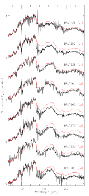
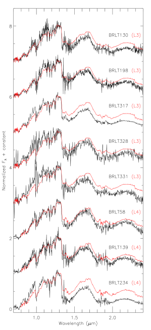
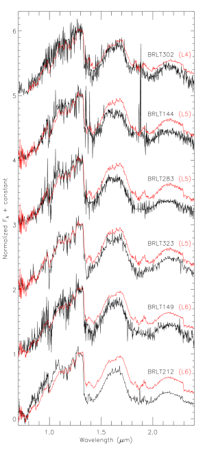
Results of the observations are presented in Table LABEL:types. For each object we present the full name, the short ID that will be used in the rest of the paper (see ADJ13 for details), the UKIDSS and SDSS photometry used for candidate selection, and the spectral type derived (see Section 3.1). The spectra of our sample are presented in Fig. 1 - 5, sorted in descending order of spectral type (from early to late). Additional SDSS and WISE photometry can be found in Appendix B.

We note that the red-optical portion of the spectra (i.e. at wavelengths shorter than 1 $\mu$ m) tend to be noisier than the infrared portion. In some objects in particular (e.g. BRLT236 and BRLT285) there appear to be strange narrow and broad features, that are due to imperfect background subtraction and/or bad pixels filtering.

3.1 Spectral classification

Spectral types for the targets were determined via $\chi^{2}$ fitting with standard templates. The template spectra were taken from the SpeX-Prism online library¹¹1http://pono.ucsd.edu/ $\sim$ adam/browndwarfs/spexprism. Each of the targets was smoothed down to the resolution of the templates (R=120), and we excluded the noisy telluric bands when computing the statistic. We visually inspected the three best fit templates to check the accuracy of the fit and to identify possible peculiar objects (see Section 3.3). The spectral types obtained are listed in the second from last column of Table LABEL:types. The uncertainty on the spectral types was determined from the width of the $\chi^{2}$ distribution.

Unsurprisingly however, a number of objects in the sample did not provide good fits when compared to the standard templates. We discuss in the following sections how we identified the peculiar objects and how we assigned their spectral types.

Refer to caption — Figure 1: The Xshooter spectra of the objects presented here, sorted in ascending order of spectral type (M8.0 $-$ L1.0). All spectra are normallized at 1.28 $\mu$ m and offset vertically by increments of one flux unit.

Name	ID	Y	J	H	K	$i$	$z$	Spectral type	Ref.
ULAS J000613.24+154020.7	BRLT1	18.954 $\pm$ 0.079	17.876 $\pm$ 0.052	16.713 $\pm$ 0.037	16.143 $\pm$ 0.036	24.161 $\pm$ 0.694	20.609 $\pm$ 0.177	L9.0 $\pm$ 0.5	1
ULAS J001040.57+010013.1	BRLT2	19.361 $\pm$ 0.084	18.089 $\pm$ 0.038	17.457 $\pm$ 0.067	16.710 $\pm$ 0.059	22.215 $\pm$ 0.198	20.797 $\pm$ 0.228	L1.0 $\pm$ 1.0	1
ULAS J001836.51 $-$ 002559.1	BRLT3	18.731 $\pm$ 0.080	17.668 $\pm$ 0.052	16.608 $\pm$ 0.038	$\ldots$	23.108 $\pm$ 0.287	20.274 $\pm$ 0.103	L9.0 $\pm$ 1.0	1
ULAS J002406.37+134705.3	BRLT6	19.281 $\pm$ 0.088	18.023 $\pm$ 0.044	17.337 $\pm$ 0.060	16.528 $\pm$ 0.044	24.677 $\pm$ 0.656	24.061 $\pm$ 0.386	L3.0 $\pm$ 1.0	1
ULAS J002707.24+142349.0	BRLT7	18.956 $\pm$ 0.059	17.981 $\pm$ 0.041	17.373 $\pm$ 0.058	16.862 $\pm$ 0.063	22.638 $\pm$ 0.264	20.410 $\pm$ 0.145	M8.0 $\pm$ 1.0	1
ULAS J002827.56+142349.1	BRLT8	18.947 $\pm$ 0.071	17.563 $\pm$ 0.034	16.616 $\pm$ 0.026	15.846 $\pm$ 0.026	22.788 $\pm$ 0.263	20.287 $\pm$ 0.122	L8.5 $\pm$ 0.5	1
ULAS J002912.25+145604.9	BRLT9	18.812 $\pm$ 0.077	17.559 $\pm$ 0.046	16.920 $\pm$ 0.053	16.330 $\pm$ 0.049	22.103 $\pm$ 0.149	19.966 $\pm$ 0.098	L1.0 $\pm$ 1.0	1
ULAS J003259.51+141037.1	BRLT10	17.830 $\pm$ 0.027	16.645 $\pm$ 0.016	15.689 $\pm$ 0.011	15.002 $\pm$ 0.013	23.083 $\pm$ 0.413	19.421 $\pm$ 0.069	L9.0 $\pm$ 0.5	2
ULAS J003716.06 $-$ 005404.7	BRLT12	19.449 $\pm$ 0.106	18.085 $\pm$ 0.057	17.330 $\pm$ 0.063	16.662 $\pm$ 0.053	22.592 $\pm$ 0.228	20.798 $\pm$ 0.196	L3.0 $\pm$ 1.0	1
ULAS J004355.61+141117.6	BRLT14	18.414 $\pm$ 0.039	17.327 $\pm$ 0.027	16.689 $\pm$ 0.036	16.120 $\pm$ 0.034	21.796 $\pm$ 0.119	19.748 $\pm$ 0.079	L0.0 $\pm$ 0.5	1
ULAS J004757.41+154641.4	BRLT15	19.118 $\pm$ 0.067	17.827 $\pm$ 0.050	17.164 $\pm$ 0.045	16.415 $\pm$ 0.042	$\ldots$	$\ldots$	T2.0 $\pm$ 2.0	1
ULAS J005038.20 $-$ 000336.6	BRLT16	19.032 $\pm$ 0.061	17.862 $\pm$ 0.043	17.068 $\pm$ 0.033	16.518 $\pm$ 0.050	22.544 $\pm$ 1.012	20.561 $\pm$ 0.144	L2.0 $\pm$ 1.0	1
ULAS J010036.01+062044.1	BRLT18	18.638 $\pm$ 0.051	17.768 $\pm$ 0.040	16.913 $\pm$ 0.038	16.335 $\pm$ 0.035	$\ldots$	$\ldots$	L0.0 $\pm$ 1.0	1
ULAS J010531.78+142931.5	BRLT20	19.258 $\pm$ 0.098	18.005 $\pm$ 0.053	17.461 $\pm$ 0.071	16.821 $\pm$ 0.080	22.924 $\pm$ 0.288	20.597 $\pm$ 0.164	L1.0 $\pm$ 1.0	1
ULAS J011151.89 $-$ 010534.2	BRLT21	18.637 $\pm$ 0.057	17.340 $\pm$ 0.028	16.532 $\pm$ 0.031	15.933 $\pm$ 0.031	22.297 $\pm$ 0.154	20.340 $\pm$ 0.098	L3.5 $\pm$ 0.5	1
ULAS J011249.67+153657.6	BRLT22	19.005 $\pm$ 0.092	17.996 $\pm$ 0.056	17.408 $\pm$ 0.037	16.856 $\pm$ 0.055	$\ldots$	$\ldots$	M8.0 $\pm$ 0.5	1
ULAS J011645.47+144335.3	BRLT24	19.309 $\pm$ 0.085	17.960 $\pm$ 0.054	17.007 $\pm$ 0.034	16.300 $\pm$ 0.038	$\ldots$	$\ldots$	L3.5 $\pm$ 0.5	1
ULAS J012743.58+135421.3	BRLT26	17.967 $\pm$ 0.034	16.772 $\pm$ 0.018	15.913 $\pm$ 0.015	15.184 $\pm$ 0.014	22.195 $\pm$ 0.170	19.626 $\pm$ 0.067	L5.5 $\pm$ 0.5	3
ULAS J012814.40 $-$ 004153.5	BRLT27	18.465 $\pm$ 0.055	17.592 $\pm$ 0.044	16.899 $\pm$ 0.030	16.487 $\pm$ 0.044	24.132 $\pm$ 0.445	20.485 $\pm$ 0.111	T0.0 $\pm$ 0.5	1
ULAS J012906.88+011350.4	BRLT28	19.315 $\pm$ 0.108	18.138 $\pm$ 0.073	17.229 $\pm$ 0.060	16.275 $\pm$ 0.039	$\ldots$	$\ldots$	L6.0 $\pm$ 0.5	$\ldots$
ULAS J013243.81+055232.2	BRLT30	17.764 $\pm$ 0.024	16.414 $\pm$ 0.013	15.481 $\pm$ 0.011	14.750 $\pm$ 0.010	21.328 $\pm$ 0.090	19.303 $\pm$ 0.066	L5.0 $\pm$ 0.5	1
ULAS J013619.79+071737.9	BRLT31	19.460 $\pm$ 0.087	18.009 $\pm$ 0.044	17.101 $\pm$ 0.044	16.474 $\pm$ 0.040	$\ldots$	$\ldots$	L4.0 $\pm$ 1.0	1
ULAS J013807.67 $-$ 010417.0	BRLT32	19.320 $\pm$ 0.114	18.006 $\pm$ 0.054	17.332 $\pm$ 0.036	$\ldots$	22.403 $\pm$ 0.152	20.816 $\pm$ 0.163	L1.5 $\pm$ 0.5	1
ULAS J014103.30+131832.6	BRLT33	19.454 $\pm$ 0.094	17.946 $\pm$ 0.041	17.095 $\pm$ 0.052	16.578 $\pm$ 0.044	22.404 $\pm$ 0.361	20.532 $\pm$ 0.186	L3.5 $\pm$ 0.5	1
ULAS J014811.69+140028.4	BRLT35	19.095 $\pm$ 0.072	17.972 $\pm$ 0.051	17.164 $\pm$ 0.050	16.551 $\pm$ 0.049	21.331 $\pm$ 0.096	21.487 $\pm$ 0.390	M9.5 $\pm$ 0.5	1
ULAS J014927.11+144108.2	BRLT37	19.304 $\pm$ 0.091	18.039 $\pm$ 0.050	17.099 $\pm$ 0.048	16.317 $\pm$ 0.039	23.488 $\pm$ 0.555	20.589 $\pm$ 0.159	L5.0 $\pm$ 0.5	1
ULAS J015142.09+124429.3	BRLT38	17.404 $\pm$ 0.020	16.388 $\pm$ 0.012	15.597 $\pm$ 0.012	15.288 $\pm$ 0.013	$\ldots$	$\ldots$	T0.0 $\pm$ 0.5	2
ULAS J015144.10+134645.8	BRLT39	18.904 $\pm$ 0.063	17.662 $\pm$ 0.035	16.839 $\pm$ 0.037	16.094 $\pm$ 0.032	23.175 $\pm$ 0.373	20.281 $\pm$ 0.135	L5.0 $\pm$ 1.0	1
ULAS J020002.96+065808.1	BRLT42	19.111 $\pm$ 0.069	17.935 $\pm$ 0.042	17.203 $\pm$ 0.044	16.717 $\pm$ 0.044	$\ldots$	$\ldots$	M9.0 $\pm$ 0.5	1
ULAS J020333.34 $-$ 010812.4	BRLT44	18.993 $\pm$ 0.085	17.693 $\pm$ 0.040	16.887 $\pm$ 0.033	16.268 $\pm$ 0.032	24.025 $\pm$ 0.444	20.468 $\pm$ 0.115	L5.0 $\pm$ 1.0	4
ULAS J020529.62+142114.0	BRLT45	19.141 $\pm$ 0.065	17.993 $\pm$ 0.039	17.266 $\pm$ 0.034	16.932 $\pm$ 0.064	25.173 $\pm$ 0.604	20.699 $\pm$ 0.189	T1.0 $\pm$ 0.5	1
ULAS J020604.27+054958.8	BRLT46	18.978 $\pm$ 0.070	17.915 $\pm$ 0.045	17.412 $\pm$ 0.069	16.801 $\pm$ 0.061	22.314 $\pm$ 1.037	20.391 $\pm$ 0.143	L0.5 $\pm$ 0.5	1
ULAS J024703.40 $-$ 010700.8	BRLT48	19.192 $\pm$ 0.089	17.766 $\pm$ 0.045	16.827 $\pm$ 0.036	15.993 $\pm$ 0.027	$\ldots$	$\ldots$	L4.5 $\pm$ 0.5	1
ULAS J025244.10+010617.9	BRLT49	19.102 $\pm$ 0.061	18.150 $\pm$ 0.050	17.541 $\pm$ 0.046	17.068 $\pm$ 0.070	$\ldots$	$\ldots$	M9.0 $\pm$ 0.5	$\ldots$
ULAS J025545.28+061655.7	BRLT50	19.153 $\pm$ 0.071	17.992 $\pm$ 0.047	18.669 $\pm$ 0.177	$\ldots$	$\ldots$	$\ldots$	T6.0 $\pm$ 0.5	5
ULAS J025940.95+054934.8	BRLT51	19.279 $\pm$ 0.079	18.024 $\pm$ 0.045	17.189 $\pm$ 0.044	16.480 $\pm$ 0.038	$\ldots$	$\ldots$	L3.0 $\pm$ 1.0	1
ULAS J031451.72+045346.2	BRLT52	18.592 $\pm$ 0.045	17.302 $\pm$ 0.025	16.388 $\pm$ 0.019	15.589 $\pm$ 0.018	22.369 $\pm$ 1.032	20.367 $\pm$ 0.123	L5.5 $\pm$ 0.5	1
ULAS J031959.75+061740.7	BRLT56	19.243 $\pm$ 0.085	17.785 $\pm$ 0.038	17.034 $\pm$ 0.034	16.396 $\pm$ 0.039	$\ldots$	$\ldots$	L1.5 $\pm$ 1.0	1
ULAS J032042.15+061837.1	BRLT57	19.273 $\pm$ 0.087	18.059 $\pm$ 0.048	17.480 $\pm$ 0.050	16.905 $\pm$ 0.061	22.424 $\pm$ 0.311	20.489 $\pm$ 0.190	L0.0 $\pm$ 1.0	1
ULAS J032143.05+054524.3	BRLT58	18.557 $\pm$ 0.052	17.333 $\pm$ 0.027	16.608 $\pm$ 0.024	15.967 $\pm$ 0.025	22.419 $\pm$ 0.253	20.077 $\pm$ 0.110	L4.0 $\pm$ 1.0	1
ULAS J032353.82+061352.3	BRLT60	19.004 $\pm$ 0.068	17.639 $\pm$ 0.034	16.989 $\pm$ 0.031	16.313 $\pm$ 0.034	$\ldots$	$\ldots$	L1.0 $\pm$ 1.0	1
ULAS J033005.72+055653.4	BRLT62	19.512 $\pm$ 0.107	17.948 $\pm$ 0.045	16.843 $\pm$ 0.032	15.948 $\pm$ 0.024	$\ldots$	$\ldots$	L5.0 $\pm$ 1.0	1
ULAS J033027.97+053626.6	BRLT63	19.219 $\pm$ 0.076	18.108 $\pm$ 0.050	17.569 $\pm$ 0.058	16.716 $\pm$ 0.046	$\ldots$	$\ldots$	L1.0 $\pm$ 0.5	$\ldots$
ULAS J033036.84+042657.7	BRLT64	18.619 $\pm$ 0.039	17.293 $\pm$ 0.023	16.444 $\pm$ 0.019	15.749 $\pm$ 0.019	22.139 $\pm$ 0.153	19.984 $\pm$ 0.095	L4.0 $\pm$ 0.5	1
ULAS J033734.61+050026.9	BRLT65	19.203 $\pm$ 0.078	18.122 $\pm$ 0.054	17.486 $\pm$ 0.055	16.872 $\pm$ 0.058	$\ldots$	$\ldots$	M9.0 $\pm$ 0.5	$\ldots$
ULAS J034150.21+042324.9	BRLT66	18.288 $\pm$ 0.032	16.848 $\pm$ 0.016	15.947 $\pm$ 0.012	15.198 $\pm$ 0.012	21.902 $\pm$ 0.175	19.778 $\pm$ 0.095	L5.0 $\pm$ 0.5	1
ULAS J080055.05+193838.1	BRLT67	18.993 $\pm$ 0.053	17.713 $\pm$ 0.025	16.960 $\pm$ 0.030	16.247 $\pm$ 0.028	22.402 $\pm$ 0.205	20.583 $\pm$ 0.115	L1.0 $\pm$ 0.5	$\ldots$
ULAS J080441.05+182611.6	BRLT68	18.815 $\pm$ 0.052	17.568 $\pm$ 0.025	16.541 $\pm$ 0.020	15.834 $\pm$ 0.019	23.114 $\pm$ 0.302	20.151 $\pm$ 0.095	L5.0 $\pm$ 0.5	$\ldots$
ULAS J082428.08+055742.5	BRLT69	18.724 $\pm$ 0.055	17.492 $\pm$ 0.030	16.891 $\pm$ 0.031	16.258 $\pm$ 0.029	22.493 $\pm$ 0.221	20.177 $\pm$ 0.095	L1.0 $\pm$ 0.5	$\ldots$
ULAS J083258.66+011241.9	BRLT71	19.256 $\pm$ 0.070	17.997 $\pm$ 0.045	17.138 $\pm$ 0.053	16.549 $\pm$ 0.044	$\ldots$	$\ldots$	L1.5 $\pm$ 0.5	$\ldots$
ULAS J083334.60 $-$ 014454.7	BRLT72	18.674 $\pm$ 0.055	17.703 $\pm$ 0.032	17.011 $\pm$ 0.034	16.388 $\pm$ 0.038	22.463 $\pm$ 0.380	20.218 $\pm$ 0.148	M9.0 $\pm$ 0.5	$\ldots$
ULAS J083842.51+081700.5	BRLT73	18.928 $\pm$ 0.056	17.720 $\pm$ 0.024	17.038 $\pm$ 0.027	16.338 $\pm$ 0.032	22.120 $\pm$ 0.136	20.653 $\pm$ 0.162	L1.0 $\pm$ 0.5	$\ldots$
ULAS J084302.02+001246.9	BRLT74	18.792 $\pm$ 0.057	17.758 $\pm$ 0.036	16.799 $\pm$ 0.032	16.288 $\pm$ 0.033	23.254 $\pm$ 0.396	20.331 $\pm$ 0.141	L9.5 $\pm$ 1.0	$\ldots$
ULAS J084410.65 $-$ 015944.2	BRLT75	19.058 $\pm$ 0.077	18.017 $\pm$ 0.048	17.438 $\pm$ 0.050	16.825 $\pm$ 0.055	23.011 $\pm$ 0.282	20.619 $\pm$ 0.175	M9.0 $\pm$ 1.0	$\ldots$
ULAS J084710.35+020413.3	BRLT76	19.777 $\pm$ 0.115	18.182 $\pm$ 0.050	17.156 $\pm$ 0.037	16.406 $\pm$ 0.039	$\ldots$	$\ldots$	L5.5 $\pm$ 0.5	$\ldots$
ULAS J084849.71+071512.0	BRLT78	18.956 $\pm$ 0.068	18.021 $\pm$ 0.031	17.417 $\pm$ 0.032	16.758 $\pm$ 0.038	$\ldots$	$\ldots$	L1.0 $\pm$ 0.5	$\ldots$
ULAS J085035.45+062152.7	BRLT81	19.158 $\pm$ 0.085	18.080 $\pm$ 0.042	17.396 $\pm$ 0.064	17.006 $\pm$ 0.053	$\ldots$	$\ldots$	M9.0 $\pm$ 0.5	$\ldots$
ULAS J085311.68+032147.7	BRLT82	19.119 $\pm$ 0.092	17.905 $\pm$ 0.067	17.040 $\pm$ 0.038	16.432 $\pm$ 0.039	22.873 $\pm$ 0.329	20.495 $\pm$ 0.180	L1.0 $\pm$ 0.5	$\ldots$
ULAS J085540.39 $-$ 021923.9	BRLT83	18.978 $\pm$ 0.058	18.159 $\pm$ 0.052	17.433 $\pm$ 0.051	16.829 $\pm$ 0.054	$\ldots$	$\ldots$	M8.0 $\pm$ 0.5	$\ldots$
ULAS J085559.77+003048.3	BRLT84	18.954 $\pm$ 0.054	17.541 $\pm$ 0.023	16.777 $\pm$ 0.020	15.998 $\pm$ 0.022	22.059 $\pm$ 0.159	20.358 $\pm$ 0.131	L3.5 $\pm$ 0.5	$\ldots$
ULAS J085931.39+063600.6	BRLT85	19.012 $\pm$ 0.050	18.077 $\pm$ 0.027	17.588 $\pm$ 0.070	17.191 $\pm$ 0.059	$\ldots$	$\ldots$	M8.0 $\pm$ 0.5	$\ldots$
ULAS J090521.61+100654.9	BRLT87	18.202 $\pm$ 0.031	17.082 $\pm$ 0.018	16.389 $\pm$ 0.021	16.074 $\pm$ 0.024	23.327 $\pm$ 0.325	19.969 $\pm$ 0.081	T0.0 $\pm$ 0.5	$\ldots$
ULAS J090710.26 $-$ 022145.7	BRLT88	19.216 $\pm$ 0.075	17.926 $\pm$ 0.042	17.012 $\pm$ 0.032	16.313 $\pm$ 0.038	$\ldots$	$\ldots$	L4.0 $\pm$ 1.0	$\ldots$
ULAS J091544.13+053104.1	BRLT91	18.084 $\pm$ 0.032	16.963 $\pm$ 0.016	16.582 $\pm$ 0.021	$\ldots$	23.846 $\pm$ 0.633	20.118 $\pm$ 0.138	T3.0 $\pm$ 0.5	$\ldots$
ULAS J091740.85+004254.0	BRLT92	18.716 $\pm$ 0.046	17.608 $\pm$ 0.026	16.889 $\pm$ 0.024	16.158 $\pm$ 0.028	22.693 $\pm$ 0.399	20.212 $\pm$ 0.136	L1.0 $\pm$ 0.5	$\ldots$
ULAS J092432.13+005835.6	BRLT97	19.175 $\pm$ 0.069	17.932 $\pm$ 0.028	17.263 $\pm$ 0.041	16.563 $\pm$ 0.041	22.444 $\pm$ 0.330	20.364 $\pm$ 0.168	L0.0 $\pm$ 1.0	$\ldots$
ULAS J092624.75+071140.7	BRLT98	18.527 $\pm$ 0.040	17.482 $\pm$ 0.021	17.386 $\pm$ 0.038	$\ldots$	$\ldots$	$\ldots$	T4.0 $\pm$ 0.5	6
ULAS J092646.81 $-$ 015150.0	BRLT99	18.906 $\pm$ 0.062	17.722 $\pm$ 0.042	16.785 $\pm$ 0.030	16.141 $\pm$ 0.031	$\ldots$	$\ldots$	L5.0 $\pm$ 0.5	$\ldots$
ULAS J092659.46 $-$ 005611.1	BRLT101	19.255 $\pm$ 0.092	17.972 $\pm$ 0.051	17.370 $\pm$ 0.072	16.894 $\pm$ 0.079	$\ldots$	$\ldots$	L3.0 $\pm$ 1.0	$\ldots$
ULAS J093129.56 $-$ 020902.8	BRLT102	19.140 $\pm$ 0.063	18.092 $\pm$ 0.044	17.314 $\pm$ 0.051	16.767 $\pm$ 0.058	$\ldots$	$\ldots$	L0.0 $\pm$ 0.5	$\ldots$
ULAS J093512.60+012347.4	BRLT103	18.515 $\pm$ 0.038	17.354 $\pm$ 0.024	16.595 $\pm$ 0.035	16.062 $\pm$ 0.029	22.358 $\pm$ 0.323	20.226 $\pm$ 0.631	L5.5 $\pm$ 0.5	$\ldots$
ULAS J093744.66+071903.3	BRLT104	18.986 $\pm$ 0.055	17.882 $\pm$ 0.030	17.189 $\pm$ 0.032	16.620 $\pm$ 0.038	22.234 $\pm$ 0.188	20.460 $\pm$ 0.158	M9.0 $\pm$ 0.5	$\ldots$
ULAS J093930.74+065309.8	BRLT105	18.083 $\pm$ 0.030	16.787 $\pm$ 0.013	15.864 $\pm$ 0.013	15.161 $\pm$ 0.010	21.698 $\pm$ 0.136	19.617 $\pm$ 0.076	L5.0 $\pm$ 0.5	$\ldots$
ULAS J094006.54+021051.1	BRLT106	18.583 $\pm$ 0.045	17.470 $\pm$ 0.030	16.869 $\pm$ 0.036	16.225 $\pm$ 0.032	$\ldots$	$\ldots$	M9.0 $\pm$ 0.5	$\ldots$
ULAS J094136.50+094214.2	BRLT108	18.883 $\pm$ 0.055	17.511 $\pm$ 0.026	16.459 $\pm$ 0.019	15.552 $\pm$ 0.018	23.163 $\pm$ 0.553	20.423 $\pm$ 0.230	L6.5 $\pm$ 0.5	$\ldots$
ULAS J094420.32+024422.7	BRLT111	19.407 $\pm$ 0.081	18.051 $\pm$ 0.052	17.116 $\pm$ 0.037	16.418 $\pm$ 0.033	$\ldots$	$\ldots$	L2.0 $\pm$ 0.5	$\ldots$
ULAS J094742.01+074232.3	BRLT112	18.822 $\pm$ 0.046	17.760 $\pm$ 0.020	17.063 $\pm$ 0.024	16.405 $\pm$ 0.030	22.409 $\pm$ 1.028	20.503 $\pm$ 0.188	L1.0 $\pm$ 0.5	$\ldots$
ULAS J094759.19+074304.7	BRLT113	18.831 $\pm$ 0.048	17.784 $\pm$ 0.021	17.154 $\pm$ 0.026	16.577 $\pm$ 0.036	23.940 $\pm$ 0.543	20.294 $\pm$ 0.152	M9.0 $\pm$ 0.5	$\ldots$
ULAS J095126.87+075756.8	BRLT114	18.724 $\pm$ 0.043	17.620 $\pm$ 0.024	16.635 $\pm$ 0.022	15.867 $\pm$ 0.018	22.610 $\pm$ 0.272	20.150 $\pm$ 0.126	L6.0 $\pm$ 0.5	$\ldots$
ULAS J095401.45+092213.7	BRLT116	18.899 $\pm$ 0.054	17.705 $\pm$ 0.023	17.333 $\pm$ 0.036	16.860 $\pm$ 0.047	$\ldots$	$\ldots$	T2.5 $\pm$ 0.5	$\ldots$
ULAS J095606.72+082115.7	BRLT117	19.302 $\pm$ 0.063	17.982 $\pm$ 0.034	17.097 $\pm$ 0.031	16.464 $\pm$ 0.031	23.156 $\pm$ 0.386	20.451 $\pm$ 0.173	L5.0 $\pm$ 0.5	$\ldots$
ULAS J100310.96+075220.3	BRLT119	19.085 $\pm$ 0.057	17.727 $\pm$ 0.027	16.869 $\pm$ 0.028	16.208 $\pm$ 0.025	$\ldots$	$\ldots$	L4.0 $\pm$ 0.5	$\ldots$
ULAS J100647.06+121117.2	BRLT121	18.799 $\pm$ 0.067	17.639 $\pm$ 0.028	16.965 $\pm$ 0.029	16.342 $\pm$ 0.041	22.071 $\pm$ 0.130	20.225 $\pm$ 0.092	L1.0 $\pm$ 0.5	$\ldots$
ULAS J100703.55+013017.0	BRLT122	18.963 $\pm$ 0.073	17.693 $\pm$ 0.037	16.949 $\pm$ 0.029	16.259 $\pm$ 0.032	22.266 $\pm$ 0.216	20.123 $\pm$ 0.130	L1.0 $\pm$ 0.5	$\ldots$
ULAS J100731.32+104758.8	BRLT123	18.899 $\pm$ 0.060	17.634 $\pm$ 0.034	16.851 $\pm$ 0.032	16.242 $\pm$ 0.024	22.583 $\pm$ 0.294	20.285 $\pm$ 0.147	L2.0 $\pm$ 0.5	$\ldots$
ULAS J101618.77+000028.0	BRLT129	18.673 $\pm$ 0.057	17.443 $\pm$ 0.023	16.553 $\pm$ 0.022	15.757 $\pm$ 0.019	$\ldots$	$\ldots$	L5.0 $\pm$ 1.0	$\ldots$
ULAS J101658.05 $-$ 013258.0	BRLT130	18.842 $\pm$ 0.045	17.939 $\pm$ 0.035	17.480 $\pm$ 0.044	16.989 $\pm$ 0.066	$\ldots$	$\ldots$	L3.0 $\pm$ 1.0	$\ldots$
ULAS J102109.61 $-$ 030420.2	BRLT131	17.038 $\pm$ 0.013	15.917 $\pm$ 0.007	15.578 $\pm$ 0.010	15.374 $\pm$ 0.016	23.578 $\pm$ 0.558	19.297 $\pm$ 0.049	T3.0 $\pm$ 0.5	7
ULAS J103553.67 $-$ 012126.3	BRLT133	19.008 $\pm$ 0.071	17.872 $\pm$ 0.053	17.317 $\pm$ 0.071	16.738 $\pm$ 0.057	$\ldots$	$\ldots$	M9.0 $\pm$ 0.5	$\ldots$
ULAS J104829.08+091939.4	BRLT135	17.575 $\pm$ 0.025	16.452 $\pm$ 0.017	15.966 $\pm$ 0.022	15.933 $\pm$ 0.029	24.254 $\pm$ 0.583	19.699 $\pm$ 0.078	T2.5 $\pm$ 0.5	8
ULAS J105836.92+085429.1	BRLT136	19.161 $\pm$ 0.091	18.059 $\pm$ 0.062	17.278 $\pm$ 0.050	16.765 $\pm$ 0.050	22.427 $\pm$ 0.290	20.458 $\pm$ 0.130	L1.0 $\pm$ 1.0	$\ldots$
ULAS J111929.43+002133.1	BRLT137	18.806 $\pm$ 0.049	17.502 $\pm$ 0.032	16.653 $\pm$ 0.029	15.936 $\pm$ 0.023	22.336 $\pm$ 0.203	20.180 $\pm$ 0.113	L4.5 $\pm$ 0.5	$\ldots$
ULAS J112029.65 $-$ 004440.6	BRLT138	18.227 $\pm$ 0.048	16.934 $\pm$ 0.026	16.034 $\pm$ 0.021	15.400 $\pm$ 0.018	21.631 $\pm$ 0.096	19.583 $\pm$ 0.063	L2.0 $\pm$ 1.0	$\ldots$
ULAS J112043.11+090429.8	BRLT139	19.146 $\pm$ 0.076	17.830 $\pm$ 0.041	17.143 $\pm$ 0.046	$\ldots$	$\ldots$	$\ldots$	L4.0 $\pm$ 1.0	$\ldots$
ULAS J113151.32 $-$ 003620.8	BRLT140	19.277 $\pm$ 0.080	18.078 $\pm$ 0.052	17.475 $\pm$ 0.042	16.908 $\pm$ 0.061	$\ldots$	$\ldots$	L0.0 $\pm$ 0.5	$\ldots$
ULAS J113850.09 $-$ 002451.3	BRLT142	18.130 $\pm$ 0.037	16.840 $\pm$ 0.018	15.910 $\pm$ 0.016	15.230 $\pm$ 0.013	21.715 $\pm$ 0.102	19.677 $\pm$ 0.064	L2.5 $\pm$ 0.5	$\ldots$
ULAS J114105.18+091647.6	BRLT144	18.658 $\pm$ 0.034	17.354 $\pm$ 0.016	16.685 $\pm$ 0.014	16.091 $\pm$ 0.018	22.471 $\pm$ 0.348	20.041 $\pm$ 0.135	L5.0 $\pm$ 1.0	$\ldots$
ULAS J114418.08+091025.1	BRLT145	19.199 $\pm$ 0.049	17.995 $\pm$ 0.028	17.202 $\pm$ 0.021	16.533 $\pm$ 0.024	23.104 $\pm$ 0.349	20.944 $\pm$ 0.189	L1.0 $\pm$ 0.5	$\ldots$
ULAS J115759.03+092200.6	BRLT147	17.986 $\pm$ 0.023	16.841 $\pm$ 0.015	16.440 $\pm$ 0.022	16.272 $\pm$ 0.034	25.500 $\pm$ 0.848	19.879 $\pm$ 0.144	T3.0 $\pm$ 0.5	9
ULAS J120009.69+120821.4	BRLT149	18.976 $\pm$ 0.064	17.585 $\pm$ 0.034	16.795 $\pm$ 0.029	16.216 $\pm$ 0.031	$\ldots$	$\ldots$	L6.0 $\pm$ 1.0	$\ldots$
ULAS J120315.34+095054.8	BRLT152	19.005 $\pm$ 0.053	17.937 $\pm$ 0.037	17.309 $\pm$ 0.043	16.741 $\pm$ 0.050	22.259 $\pm$ 0.162	20.684 $\pm$ 0.123	L0.0 $\pm$ 0.5	$\ldots$
ULAS J120323.74 $-$ 015655.8	BRLT153	18.817 $\pm$ 0.072	17.727 $\pm$ 0.046	17.208 $\pm$ 0.054	16.708 $\pm$ 0.058	22.382 $\pm$ 0.328	20.356 $\pm$ 0.175	L1.0 $\pm$ 0.5	$\ldots$
ULAS J120545.92+084206.8	BRLT155	18.522 $\pm$ 0.065	17.261 $\pm$ 0.037	16.357 $\pm$ 0.022	15.707 $\pm$ 0.022	22.073 $\pm$ 0.181	19.847 $\pm$ 0.102	L3.0 $\pm$ 1.0	$\ldots$
ULAS J120943.05+065333.0	BRLT159	19.461 $\pm$ 0.091	18.097 $\pm$ 0.049	17.166 $\pm$ 0.055	16.590 $\pm$ 0.053	23.362 $\pm$ 0.493	20.845 $\pm$ 0.186	L9.0 $\pm$ 0.5	$\ldots$
ULAS J121238.72+000721.9	BRLT162	16.792 $\pm$ 0.013	15.684 $\pm$ 0.008	15.037 $\pm$ 0.009	14.461 $\pm$ 0.009	20.287 $\pm$ 0.076	18.381 $\pm$ 0.041	L0.5 $\pm$ 0.5	$\ldots$
ULAS J121320.56+150235.1	BRLT163	18.776 $\pm$ 0.047	17.647 $\pm$ 0.029	16.865 $\pm$ 0.033	16.204 $\pm$ 0.035	$\ldots$	$\ldots$	L1.0 $\pm$ 0.5	$\ldots$
ULAS J121355.51+053517.1	BRLT164	18.934 $\pm$ 0.071	17.882 $\pm$ 0.044	17.617 $\pm$ 0.069	17.639 $\pm$ 0.133	$\ldots$	$\ldots$	T3.0 $\pm$ 0.5	$\ldots$
ULAS J121816.52+134953.8	BRLT165	19.147 $\pm$ 0.078	17.953 $\pm$ 0.050	17.321 $\pm$ 0.038	16.599 $\pm$ 0.043	$\ldots$	$\ldots$	L2.0 $\pm$ 0.5	$\ldots$
ULAS J122111.67+122217.0	BRLT168	19.391 $\pm$ 0.091	17.974 $\pm$ 0.041	17.092 $\pm$ 0.031	16.312 $\pm$ 0.031	22.366 $\pm$ 0.198	20.770 $\pm$ 0.185	L4.0 $\pm$ 0.5	$\ldots$
ULAS J122325.69+044827.6	BRLT171	17.681 $\pm$ 0.020	16.372 $\pm$ 0.010	15.448 $\pm$ 0.009	14.651 $\pm$ 0.008	21.467 $\pm$ 0.115	19.339 $\pm$ 0.076	L5.0 $\pm$ 0.5	$\ldots$
ULAS J123012.52+071717.9	BRLT176	18.822 $\pm$ 0.050	17.564 $\pm$ 0.029	16.794 $\pm$ 0.021	16.110 $\pm$ 0.026	22.606 $\pm$ 0.252	20.249 $\pm$ 0.126	L4.0 $\pm$ 1.0	$\ldots$
ULAS J123327.44+121952.1	BRLT179	19.006 $\pm$ 0.078	18.020 $\pm$ 0.042	18.219 $\pm$ 0.086	$\ldots$	22.338 $\pm$ 0.502	22.422 $\pm$ 0.578	T4.5 $\pm$ 0.5	6
ULAS J123433.51+010742.0	BRLT181	19.114 $\pm$ 0.103	17.823 $\pm$ 0.056	17.093 $\pm$ 0.041	16.379 $\pm$ 0.035	22.605 $\pm$ 0.265	20.578 $\pm$ 0.179	L1.0 $\pm$ 1.0	$\ldots$
ULAS J123845.96+124737.7	BRLT182	18.779 $\pm$ 0.068	17.719 $\pm$ 0.037	17.098 $\pm$ 0.037	16.668 $\pm$ 0.051	$\ldots$	$\ldots$	T3.0 $\pm$ 0.5	$\ldots$
ULAS J124052.92+112940.4	BRLT186	16.596 $\pm$ 0.010	15.509 $\pm$ 0.006	14.829 $\pm$ 0.006	14.243 $\pm$ 0.006	21.519 $\pm$ 1.459	18.195 $\pm$ 1.498	L1.0 $\pm$ 1.0	$\ldots$
ULAS J124413.03+123201.1	BRLT190	18.891 $\pm$ 0.068	17.642 $\pm$ 0.032	17.419 $\pm$ 0.046	17.455 $\pm$ 0.103	$\ldots$	$\ldots$	T4.0 $\pm$ 0.5	$\ldots$
ULAS J130435.66+154252.6	BRLT197	18.611 $\pm$ 0.035	17.189 $\pm$ 0.019	16.441 $\pm$ 0.021	15.863 $\pm$ 0.022	23.610 $\pm$ 0.405	20.210 $\pm$ 0.164	T2.0 $\pm$ 1.0	$\ldots$
ULAS J131106.96 $-$ 013742.3	BRLT198	19.004 $\pm$ 0.077	17.832 $\pm$ 0.049	17.283 $\pm$ 0.056	16.632 $\pm$ 0.043	22.491 $\pm$ 0.251	20.595 $\pm$ 0.175	L3.0 $\pm$ 1.0	$\ldots$
ULAS J131307.47+123540.7	BRLT202	18.578 $\pm$ 0.047	17.425 $\pm$ 0.025	16.908 $\pm$ 0.030	16.505 $\pm$ 0.039	23.617 $\pm$ 0.624	20.715 $\pm$ 0.177	T2.5 $\pm$ 0.5	$\ldots$
ULAS J131610.13+031205.5	BRLT203	17.998 $\pm$ 0.032	16.747 $\pm$ 0.018	16.129 $\pm$ 0.018	15.432 $\pm$ 0.019	22.831 $\pm$ 0.369	20.043 $\pm$ 0.114	T3.0 $\pm$ 1.0	$\ldots$
ULAS J132410.21+025040.6	BRLT206	19.394 $\pm$ 0.069	18.072 $\pm$ 0.043	17.254 $\pm$ 0.049	16.656 $\pm$ 0.047	22.672 $\pm$ 0.355	20.676 $\pm$ 0.184	L2.0 $\pm$ 0.5	$\ldots$
ULAS J132629.65 $-$ 003832.5	BRLT207	17.592 $\pm$ 0.018	16.221 $\pm$ 0.011	15.111 $\pm$ 0.007	14.171 $\pm$ 0.006	21.716 $\pm$ 0.104	19.074 $\pm$ 0.041	L7.0 $\pm$ 0.5	10
ULAS J132720.56+101138.5	BRLT210	18.813 $\pm$ 0.059	17.481 $\pm$ 0.025	16.580 $\pm$ 0.017	15.829 $\pm$ 0.017	22.928 $\pm$ 0.265	20.279 $\pm$ 0.104	L4.5 $\pm$ 0.5	$\ldots$
ULAS J133148.66 $-$ 011700.6	BRLT212	16.498 $\pm$ 0.009	15.330 $\pm$ 0.006	14.671 $\pm$ 0.004	14.051 $\pm$ 0.005	$\ldots$	$\ldots$	L6.0 $\pm$ 1.0	3
ULAS J134322.94 $-$ 010844.0	BRLT216	18.480 $\pm$ 0.028	17.429 $\pm$ 0.018	16.715 $\pm$ 0.016	16.224 $\pm$ 0.025	21.870 $\pm$ 0.313	20.057 $\pm$ 0.170	M9.0 $\pm$ 0.5	$\ldots$
ULAS J134403.78+083951.0	BRLT217	18.391 $\pm$ 0.042	17.258 $\pm$ 0.022	16.455 $\pm$ 0.017	15.955 $\pm$ 0.021	23.065 $\pm$ 0.325	20.005 $\pm$ 0.080	T0.0 $\pm$ 0.5	$\ldots$
ULAS J134414.90+092405.0	BRLT218	18.624 $\pm$ 0.030	17.287 $\pm$ 0.012	16.302 $\pm$ 0.016	15.460 $\pm$ 0.013	22.786 $\pm$ 0.257	20.207 $\pm$ 0.110	L6.0 $\pm$ 0.5	$\ldots$
ULAS J134436.84+110957.5	BRLT219	18.442 $\pm$ 0.046	17.218 $\pm$ 0.022	16.922 $\pm$ 0.034	16.934 $\pm$ 0.058	24.733 $\pm$ 0.519	20.649 $\pm$ 0.128	T3.0 $\pm$ 0.5	$\ldots$
ULAS J134612.77+082503.3	BRLT220	19.356 $\pm$ 0.108	18.005 $\pm$ 0.043	17.257 $\pm$ 0.037	16.500 $\pm$ 0.036	22.836 $\pm$ 0.274	20.434 $\pm$ 0.118	L2.0 $\pm$ 0.5	$\ldots$
ULAS J135556.12+085054.3	BRLT227	18.667 $\pm$ 0.051	17.297 $\pm$ 0.020	16.385 $\pm$ 0.020	15.630 $\pm$ 0.015	22.200 $\pm$ 0.145	20.281 $\pm$ 0.109	L3.0 $\pm$ 0.5	$\ldots$
ULAS J135848.63+014745.5	BRLT229	18.493 $\pm$ 0.045	17.620 $\pm$ 0.039	16.995 $\pm$ 0.034	16.520 $\pm$ 0.037	22.005 $\pm$ 0.385	20.070 $\pm$ 0.131	M8.0 $\pm$ 0.5	$\ldots$
ULAS J140152.43+090733.1	BRLT231	18.640 $\pm$ 0.045	17.320 $\pm$ 0.018	16.398 $\pm$ 0.014	15.625 $\pm$ 0.014	22.716 $\pm$ 0.218	20.288 $\pm$ 0.121	L5.0 $\pm$ 0.5	$\ldots$
ULAS J140255.67+080054.5	BRLT232	17.991 $\pm$ 0.033	16.837 $\pm$ 0.014	16.204 $\pm$ 0.021	15.706 $\pm$ 0.020	22.966 $\pm$ 0.343	19.938 $\pm$ 0.083	T2.5 $\pm$ 0.5	8
ULAS J141203.85+121609.9	BRLT234	17.540 $\pm$ 0.017	16.325 $\pm$ 0.010	15.851 $\pm$ 0.014	15.430 $\pm$ 0.015	21.322 $\pm$ 0.084	19.150 $\pm$ 0.047	L4.0 $\pm$ 1.0	$\ldots$
ULAS J141405.68+010709.3	BRLT236	18.119 $\pm$ 0.040	16.791 $\pm$ 0.024	15.958 $\pm$ 0.017	15.205 $\pm$ 0.014	21.728 $\pm$ 0.132	19.605 $\pm$ 0.086	L3.5 $\pm$ 0.5	$\ldots$
ULAS J141710.01+131737.1	BRLT237	18.051 $\pm$ 0.027	16.690 $\pm$ 0.011	15.912 $\pm$ 0.009	15.208 $\pm$ 0.010	21.678 $\pm$ 0.094	19.637 $\pm$ 0.078	L4.0 $\pm$ 0.5	$\ldots$
ULAS J142300.38+041026.4	BRLT240	18.819 $\pm$ 0.078	17.386 $\pm$ 0.037	16.549 $\pm$ 0.031	15.796 $\pm$ 0.028	22.215 $\pm$ 0.216	20.057 $\pm$ 0.143	L3.0 $\pm$ 0.5	$\ldots$
ULAS J142718.33+011206.2	BRLT243	18.832 $\pm$ 0.075	17.481 $\pm$ 0.038	16.746 $\pm$ 0.028	16.386 $\pm$ 0.041	22.676 $\pm$ 0.397	20.267 $\pm$ 0.171	T0.0 $\pm$ 0.5	$\ldots$
ULAS J143256.93+122809.2	BRLT247	18.626 $\pm$ 0.057	17.631 $\pm$ 0.035	16.911 $\pm$ 0.030	16.356 $\pm$ 0.027	$\ldots$	$\ldots$	M9.0 $\pm$ 0.5	$\ldots$
ULAS J143615.75+072056.8	BRLT249	18.524 $\pm$ 0.044	17.105 $\pm$ 0.022	16.180 $\pm$ 0.018	15.531 $\pm$ 0.019	22.546 $\pm$ 0.242	20.043 $\pm$ 0.095	L5.0 $\pm$ 0.5	$\ldots$
ULAS J143623.86+014257.6	BRLT250	18.981 $\pm$ 0.060	17.603 $\pm$ 0.036	16.785 $\pm$ 0.030	16.062 $\pm$ 0.026	22.866 $\pm$ 0.324	20.446 $\pm$ 0.167	L1.0 $\pm$ 0.5	$\ldots$
ULAS J143705.60+115930.1	BRLT251	18.856 $\pm$ 0.059	17.686 $\pm$ 0.033	17.130 $\pm$ 0.061	16.540 $\pm$ 0.038	22.402 $\pm$ 0.182	20.291 $\pm$ 0.103	L1.0 $\pm$ 0.5	$\ldots$
ULAS J144151.55+043738.5	BRLT253	18.443 $\pm$ 0.041	17.326 $\pm$ 0.028	16.784 $\pm$ 0.039	16.408 $\pm$ 0.043	$\ldots$	$\ldots$	L1.0 $\pm$ 1.0	$\ldots$
ULAS J144220.94+084945.9	BRLT254	18.601 $\pm$ 0.032	17.302 $\pm$ 0.016	16.428 $\pm$ 0.014	15.711 $\pm$ 0.015	22.443 $\pm$ 0.190	20.123 $\pm$ 0.086	L5.0 $\pm$ 0.5	$\ldots$
ULAS J144600.70+002451.4	BRLT258	16.895 $\pm$ 0.014	15.584 $\pm$ 0.007	14.657 $\pm$ 0.005	13.921 $\pm$ 0.005	20.760 $\pm$ 0.048	18.572 $\pm$ 0.046	L5.0 $\pm$ 1.0	2
ULAS J144812.93 $-$ 000018.6	BRLT260	18.870 $\pm$ 0.068	17.598 $\pm$ 0.040	17.121 $\pm$ 0.043	16.553 $\pm$ 0.053	22.480 $\pm$ 0.202	20.493 $\pm$ 0.138	L2.0 $\pm$ 1.0	$\ldots$
ULAS J145231.11+033944.0	BRLT262	19.368 $\pm$ 0.114	18.066 $\pm$ 0.058	17.194 $\pm$ 0.054	16.514 $\pm$ 0.051	$\ldots$	$\ldots$	L0.0 $\pm$ 0.5	$\ldots$
ULAS J145541.74+002224.3	BRLT265	18.864 $\pm$ 0.074	17.608 $\pm$ 0.046	16.727 $\pm$ 0.033	15.975 $\pm$ 0.027	22.460 $\pm$ 0.210	20.169 $\pm$ 0.114	L2.0 $\pm$ 0.5	$\ldots$
ULAS J150140.69 $-$ 005146.8	BRLT269	19.255 $\pm$ 0.064	17.573 $\pm$ 0.035	16.557 $\pm$ 0.026	15.618 $\pm$ 0.028	$\ldots$	$\ldots$	L7.0 $\pm$ 0.5	$\ldots$
ULAS J150531.70+010232.7	BRLT270	18.635 $\pm$ 0.043	17.441 $\pm$ 0.025	16.865 $\pm$ 0.033	16.434 $\pm$ 0.047	22.731 $\pm$ 0.244	20.100 $\pm$ 0.100	L2.0 $\pm$ 1.0	$\ldots$
ULAS J150927.83+034449.7	BRLT274	18.809 $\pm$ 0.050	17.245 $\pm$ 0.026	16.178 $\pm$ 0.017	15.262 $\pm$ 0.017	$\ldots$	$\ldots$	L2.0 $\pm$ 0.5	$\ldots$
ULAS J151114.51+060741.1	BRLT275	17.220 $\pm$ 0.016	15.878 $\pm$ 0.009	15.183 $\pm$ 0.007	14.440 $\pm$ 0.008	21.672 $\pm$ 0.102	19.201 $\pm$ 0.050	T2.0 $\pm$ 2.0	8
ULAS J151145.75 $-$ 021726.5	BRLT276	18.585 $\pm$ 0.041	17.420 $\pm$ 0.037	16.779 $\pm$ 0.036	16.235 $\pm$ 0.040	$\ldots$	$\ldots$	L0.0 $\pm$ 0.5	$\ldots$
ULAS J151355.05 $-$ 013300.6	BRLT279	17.899 $\pm$ 0.030	16.758 $\pm$ 0.018	16.072 $\pm$ 0.018	15.470 $\pm$ 0.019	21.478 $\pm$ 0.095	19.309 $\pm$ 0.067	L1.0 $\pm$ 0.5	$\ldots$
ULAS J151603.00+025927.7	BRLT281	17.959 $\pm$ 0.033	16.877 $\pm$ 0.022	16.075 $\pm$ 0.017	15.437 $\pm$ 0.017	22.997 $\pm$ 0.383	19.709 $\pm$ 0.078	T0.0 $\pm$ 0.5	4
ULAS J151649.84+083607.1	BRLT283	18.741 $\pm$ 0.041	17.349 $\pm$ 0.019	16.705 $\pm$ 0.025	16.258 $\pm$ 0.029	22.693 $\pm$ 0.213	20.374 $\pm$ 0.098	L5.0 $\pm$ 1.0	$\ldots$
ULAS J151821.34+085517.5	BRLT285	18.618 $\pm$ 0.031	17.419 $\pm$ 0.014	16.530 $\pm$ 0.022	15.777 $\pm$ 0.017	22.553 $\pm$ 0.215	20.194 $\pm$ 0.091	L5.0 $\pm$ 0.5	$\ldots$
ULAS J152103.14+013143.2	BRLT287	17.339 $\pm$ 0.018	16.097 $\pm$ 0.010	15.679 $\pm$ 0.009	15.568 $\pm$ 0.015	24.750 $\pm$ 0.515	19.606 $\pm$ 0.064	T3.0 $\pm$ 0.5	4
ULAS J152502.10+083344.0	BRLT290	18.249 $\pm$ 0.031	17.170 $\pm$ 0.018	16.618 $\pm$ 0.021	16.217 $\pm$ 0.028	22.844 $\pm$ 0.214	20.367 $\pm$ 0.101	T2.0 $\pm$ 0.5	$\ldots$
ULAS J153128.47+073755.0	BRLT295	17.852 $\pm$ 0.023	16.607 $\pm$ 0.011	16.022 $\pm$ 0.013	15.445 $\pm$ 0.014	21.547 $\pm$ 0.096	19.458 $\pm$ 0.071	L4.0 $\pm$ 2.0	$\ldots$
ULAS J153156.73+033605.9	BRLT296	18.466 $\pm$ 0.053	17.285 $\pm$ 0.036	16.401 $\pm$ 0.017	15.749 $\pm$ 0.019	22.327 $\pm$ 0.220	19.950 $\pm$ 0.119	L4.0 $\pm$ 0.5	$\ldots$
ULAS J153256.84 $-$ 012511.0	BRLT297	19.129 $\pm$ 0.105	17.647 $\pm$ 0.041	16.827 $\pm$ 0.039	16.056 $\pm$ 0.032	$\ldots$	$\ldots$	L4.5 $\pm$ 0.5	$\ldots$
ULAS J154038.87 $-$ 001256.7	BRLT299	17.838 $\pm$ 0.022	16.625 $\pm$ 0.015	15.814 $\pm$ 0.010	15.175 $\pm$ 0.011	21.660 $\pm$ 0.105	19.343 $\pm$ 0.056	L4.0 $\pm$ 1.0	$\ldots$
ULAS J154319.80+080446.3	BRLT301	18.863 $\pm$ 0.050	17.655 $\pm$ 0.027	16.937 $\pm$ 0.039	16.537 $\pm$ 0.040	21.991 $\pm$ 0.139	20.335 $\pm$ 0.143	L1.0 $\pm$ 0.5	$\ldots$
ULAS J154448.83+094256.9	BRLT302	18.803 $\pm$ 0.053	17.671 $\pm$ 0.036	16.980 $\pm$ 0.022	16.367 $\pm$ 0.025	22.722 $\pm$ 0.284	20.259 $\pm$ 0.146	L4.0 $\pm$ 1.0	$\ldots$
ULAS J215700.47+005614.5	BRLT305	19.258 $\pm$ 0.125	17.852 $\pm$ 0.047	16.873 $\pm$ 0.043	16.105 $\pm$ 0.031	22.274 $\pm$ 0.149	20.618 $\pm$ 0.130	L5.5 $\pm$ 1.0	1
ULAS J215920.00+003309.7	BRLT306	19.091 $\pm$ 0.112	17.734 $\pm$ 0.045	16.993 $\pm$ 0.048	16.365 $\pm$ 0.040	23.008 $\pm$ 0.316	20.498 $\pm$ 1.056	L4.5 $\pm$ 0.5	1
ULAS J220917.12 $-$ 005259.9	BRLT307	19.348 $\pm$ 0.096	18.006 $\pm$ 0.049	17.262 $\pm$ 0.070	16.636 $\pm$ 0.056	22.796 $\pm$ 0.333	20.482 $\pm$ 0.143	L1.0 $\pm$ 0.5	1
ULAS J221904.07+063059.1	BRLT308	19.523 $\pm$ 0.088	18.124 $\pm$ 0.051	17.208 $\pm$ 0.049	16.447 $\pm$ 0.045	$\ldots$	$\ldots$	L5.0 $\pm$ 0.5	$\ldots$
ULAS J222710.91 $-$ 004547.3	BRLT309	19.503 $\pm$ 0.110	18.116 $\pm$ 0.061	16.616 $\pm$ 0.029	15.322 $\pm$ 0.017	$\ldots$	$\ldots$	L7.0 $\pm$ 0.5	11
ULAS J222958.30+010217.2	BRLT311	19.106 $\pm$ 0.066	17.885 $\pm$ 0.039	17.499 $\pm$ 0.054	17.218 $\pm$ 0.095	$\ldots$	$\ldots$	T3.0 $\pm$ 0.5	1
ULAS J223347.82+002214.0	BRLT312	19.119 $\pm$ 0.068	18.068 $\pm$ 0.048	17.361 $\pm$ 0.063	16.641 $\pm$ 0.050	21.934 $\pm$ 0.123	21.517 $\pm$ 0.328	T0.0 $\pm$ 0.5	1
ULAS J223636.89+011132.3	BRLT313	18.447 $\pm$ 0.039	17.109 $\pm$ 0.021	16.239 $\pm$ 0.017	15.474 $\pm$ 0.017	22.179 $\pm$ 0.144	20.149 $\pm$ 0.089	L3.5 $\pm$ 0.5	1
ULAS J223756.91+071656.8	BRLT314	18.871 $\pm$ 0.064	17.491 $\pm$ 0.035	16.447 $\pm$ 0.023	15.656 $\pm$ 0.022	23.195 $\pm$ 0.444	20.464 $\pm$ 0.116	L7.5 $\pm$ 0.5	1
ULAS J224051.81+000822.0	BRLT315	19.276 $\pm$ 0.078	17.819 $\pm$ 0.036	17.117 $\pm$ 0.046	16.577 $\pm$ 0.049	22.286 $\pm$ 0.146	20.258 $\pm$ 0.114	L1.0 $\pm$ 1.0	1
ULAS J224922.85+071527.9	BRLT316	19.638 $\pm$ 0.107	18.089 $\pm$ 0.051	17.542 $\pm$ 0.062	16.855 $\pm$ 0.057	$\ldots$	$\ldots$	L1.0 $\pm$ 0.5	1
ULAS J225016.39+080822.4	BRLT317	16.670 $\pm$ 0.009	15.503 $\pm$ 0.005	15.048 $\pm$ 0.006	14.513 $\pm$ 0.007	20.357 $\pm$ 0.041	18.243 $\pm$ 0.029	L3.0 $\pm$ 1.0	1
ULAS J225114.89 $-$ 000724.4	BRLT318	19.209 $\pm$ 0.096	17.951 $\pm$ 0.059	17.353 $\pm$ 0.073	16.493 $\pm$ 0.048	22.114 $\pm$ 0.167	21.147 $\pm$ 0.292	L1.0 $\pm$ 0.5	1
ULAS J225624.82+062152.9	BRLT319	19.444 $\pm$ 0.098	18.139 $\pm$ 0.051	17.928 $\pm$ 0.079	17.646 $\pm$ 0.100	$\ldots$	$\ldots$	T3.0 $\pm$ 0.5	$\ldots$
ULAS J225630.91+072439.0	BRLT320	19.421 $\pm$ 0.070	17.944 $\pm$ 0.032	17.261 $\pm$ 0.036	16.732 $\pm$ 0.043	23.100 $\pm$ 0.330	20.649 $\pm$ 0.184	M9.0 $\pm$ 0.5	1
ULAS J230203.04+070038.8	BRLT321	18.954 $\pm$ 0.067	17.625 $\pm$ 0.032	17.379 $\pm$ 0.047	17.514 $\pm$ 0.088	$\ldots$	$\ldots$	T4.0 $\pm$ 0.5	1
ULAS J230358.64+005807.3	BRLT322	19.029 $\pm$ 0.070	17.821 $\pm$ 0.030	16.989 $\pm$ 0.060	16.151 $\pm$ 0.036	23.272 $\pm$ 0.416	20.677 $\pm$ 0.191	L5.0 $\pm$ 0.5	1
ULAS J230424.80+130111.3	BRLT323	18.002 $\pm$ 0.023	16.692 $\pm$ 0.012	15.926 $\pm$ 0.021	15.203 $\pm$ 0.015	21.527 $\pm$ 0.109	19.470 $\pm$ 0.065	L5.0 $\pm$ 1.0	1
ULAS J230434.41+080401.4	BRLT325	19.119 $\pm$ 0.072	17.888 $\pm$ 0.046	17.478 $\pm$ 0.076	17.218 $\pm$ 0.090	$\ldots$	$\ldots$	T2.0 $\pm$ 1.0	1
ULAS J231236.55+000602.3	BRLT328	18.955 $\pm$ 0.059	17.654 $\pm$ 0.022	17.051 $\pm$ 0.030	16.408 $\pm$ 0.043	22.348 $\pm$ 0.155	20.276 $\pm$ 0.114	L3.0 $\pm$ 1.0	1
ULAS J231645.70+010012.5	BRLT330	19.100 $\pm$ 0.075	17.949 $\pm$ 0.030	17.263 $\pm$ 0.065	16.700 $\pm$ 0.062	23.017 $\pm$ 0.379	21.075 $\pm$ 0.269	L2.0 $\pm$ 1.0	1
ULAS J232122.72 $-$ 004557.3	BRLT331	19.403 $\pm$ 0.085	18.004 $\pm$ 0.043	17.604 $\pm$ 0.065	17.126 $\pm$ 0.065	22.964 $\pm$ 0.272	20.526 $\pm$ 0.123	L3.0 $\pm$ 1.0	1
ULAS J232259.58+000541.5	BRLT332	19.163 $\pm$ 0.070	18.009 $\pm$ 0.042	17.264 $\pm$ 0.050	16.855 $\pm$ 0.055	22.706 $\pm$ 0.201	20.540 $\pm$ 0.137	L3.0 $\pm$ 1.0	1
ULAS J232315.39+071931.0	BRLT333	18.501 $\pm$ 0.036	17.301 $\pm$ 0.022	16.550 $\pm$ 0.027	16.200 $\pm$ 0.031	23.727 $\pm$ 0.354	20.349 $\pm$ 0.104	T2.0 $\pm$ 0.5	1
ULAS J232715.67+151729.5	BRLT334	17.541 $\pm$ 0.020	16.203 $\pm$ 0.011	15.357 $\pm$ 0.013	14.684 $\pm$ 0.010	21.297 $\pm$ 0.073	19.171 $\pm$ 0.041	L3.5 $\pm$ 0.5	1
ULAS J232732.12+010252.7	BRLT335	19.261 $\pm$ 0.070	18.068 $\pm$ 0.047	17.236 $\pm$ 0.063	16.608 $\pm$ 0.060	$\ldots$	$\ldots$	L4.0 $\pm$ 1.0	1
ULAS J233002.13+140329.9	BRLT338	18.593 $\pm$ 0.061	17.367 $\pm$ 0.035	16.792 $\pm$ 0.046	16.105 $\pm$ 0.036	$\ldots$	$\ldots$	L1.0 $\pm$ 1.0	1
ULAS J233942.81+075327.2	BRLT340	19.840 $\pm$ 0.128	18.134 $\pm$ 0.048	17.337 $\pm$ 0.065	16.541 $\pm$ 0.047	$\ldots$	$\ldots$	L4.0 $\pm$ 0.5	$\ldots$
ULAS J234716.98 $-$ 011009.1	BRLT343	18.817 $\pm$ 0.063	17.571 $\pm$ 0.033	16.720 $\pm$ 0.027	15.899 $\pm$ 0.026	22.616 $\pm$ 0.236	20.268 $\pm$ 0.120	L9.0 $\pm$ 1.0	1
ULAS J235618.01+075420.4	BRLT344	19.602 $\pm$ 0.093	18.089 $\pm$ 0.049	16.986 $\pm$ 0.047	16.215 $\pm$ 0.036	$\ldots$	$\ldots$	T0.0 $\pm$ 1.0	1

Table 1: The objects observed. YJHK magnitudes are from the UKIDSS LAS DR7, while

iz

magnitudes are from the SDSS DR7. The spectral types are derived in Section 3.1. Discovery reference: (1) Day-Jones et al. (2013); (2) Geballe et al. (2002); (3) Hawley et al. (2002); (4) Knapp et al. (2004); (5) Burningham et al. (2013); (6) Burningham et al. (2010); (7) Leggett et al. (2000); (8) Chiu et al. (2006); (9) Pinfield et al. (2008); (10) Fan et al. (2000); (11) Marocco et al. (2014). If no discovery reference is listed, the object was previously unpublished.

3.2 Identification of unresolved binaries

One possible source of peculiarity in the spectra of brown dwarfs is binarity. Unresolved binaries are in fact characterized by odd spectra, which are the result of the combination of the two components of the system. This is particularly true in L/T transition pairs, where the two components have comparable brightness but significantly different spectra (e.g. Burgasser et al., 2010).

In order to select binary candidates within the sample, we followed the method described by Burgasser et al. (2010), who used a combination of index-index and index-spectral type diagrams to define a number of criteria based on the distribution of known unresolved binaries, designed to minimize the number of false positives. The selection is therefore not complete. Objects that match two of the six criteria are called “weak candidates” while objects that match three or more criteria are called “strong candidates”. The indices used are summarized in Table 2, while the criteria applied are listed in Table 3.

With this technique we were able to identify 27 binary candidates, consisting of 17 weak candidates and 10 strong candidates, which are listed in Table 4. The index-index and index-spectral type diagram used are presented in Figure 6, where strong candidates are marked with a diamond and weak candidates are marked with an asterisk.

Index	Numerator	Denominator	Feature
	Range	Range
H₂O-J	1.14-1.165	1.26-1.285	1.15 $\mu$ m H₂O
H₂O-H	1.48-1.52	1.56-1.60	1.4 $\mu$ m H₂O
H₂O-K	1.975-1.995	2.08-2.10	1.9 $\mu$ m H₂O
CH₄-J	1.315-1.34	1.26-1.285	1.32 $\mu$ m CH₄
CH₄-H	1.635-1.675	1.56-1.60	1.65 $\mu$ m CH₄
CH₄-K	2.215-2.255	2.08-2.12	2.2 $\mu$ m CH₄
K/J	2.060-2.10	1.25-1.29	J-K colour
H-dip	1.61-1.64	1.56-1.59 + 1.66-1.69	1.65 $\mu$ m CH₄

Table 2: The spectral indices used to identify unresolved binary candidates. All the indices are defined in Burgasser et al. (2006) except for H-dip which is defined in Burgasser et al. (2010).

Abscissa	Ordinate	Inflection Points
		(x,y)
H₂O-J	H₂O-K	(0.325,0.5),(0.65,0.7)
CH₄-H	CH₄O-K	(0.6,0.35),(1,0.775)
CH₄-H	K/J	(0.65,0.25),(1,0.375)
H₂O-H	H-dip	(0.5,0.49),(0.875,0.49)
SpT	H₂O-J/H₂O-H	(L8.5,0.925),(T1.5,0.925),(T3.5,0.85)
SpT	H₂O-J/CH₄-K	(L8.5,0.625),(T4.5,0.825)

Table 3: The selection criteria used to identify unresolved binary candidates. Inflection points are defined in Burgasser et al. (2010).

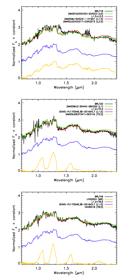
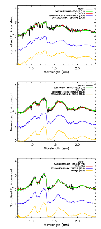
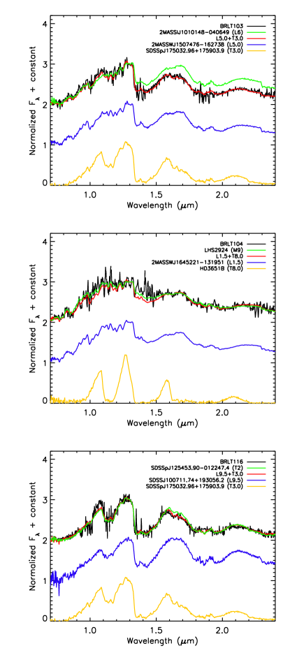
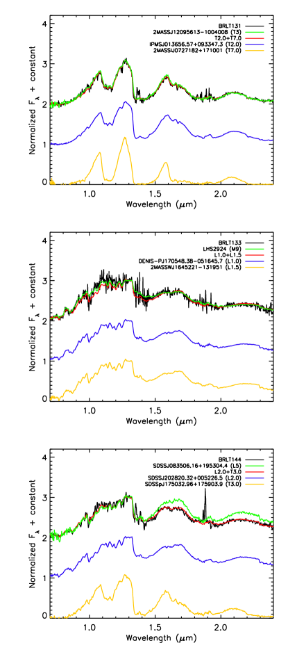
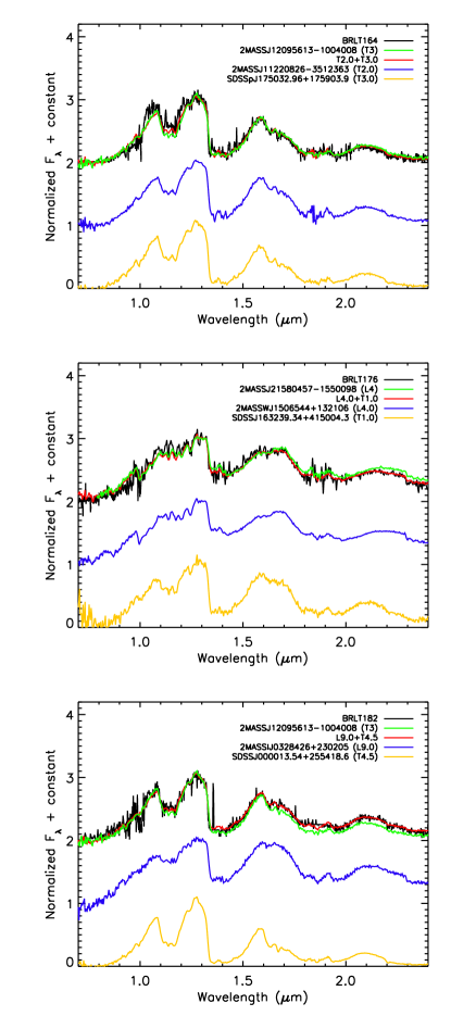
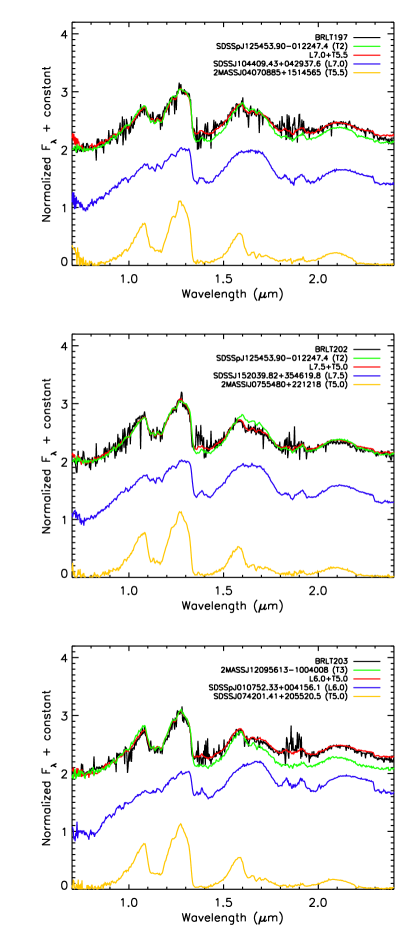
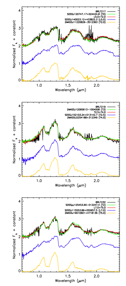
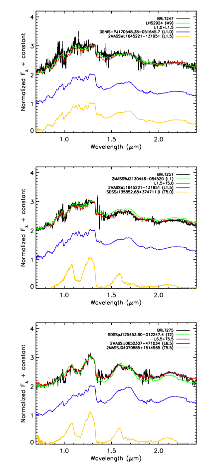
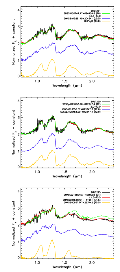
To deconvolve the spectra of the binary candidates and determine the types of the potential components we used the technique described in ADJ13. We created a library of synthetic unresolved binaries combining the spectral templates taken from the already mentioned SpeX-Prism library. All the templates were scaled to a common flux level using the $M_{J}$ -spectral type relation defined in Marocco et al. (2010, excluding both known and possible binaries) and combined. Each candidate was then fitted with this new set of templates using a $\chi^{2}$ fitting technique, after normalizing both the candidate and the template at 1.28 $\mu$ m. The fit are presented in Figure 7 $-$ 11. The results of this fit were compared to the results obtained using the standard templates with a one-sided F test, to assess the statistical significance of the deconvolution. If the ratio of the two chi-squared fits ( $\eta$ ) is greater than the critical value ( $\eta_{\rm crit}=1.15$ ), this represents a $99\%$ significance that the combined template fit is better than the standard template alone. The results are shown in Table 4 where for each target we present the best fit standard template (with the associated $\chi^{2}$ ), the best fit combined template (with $\chi^{2}$ ) and the $\eta$ value of the F test. As one can see, 13 out of 27 dwarfs give a statistically “better fit” using combined templates ( $\eta>$ 1.15) and are therefore the strongest binary candidates.

Three of these candidates have previously been identified as binaries or binary candidates. BRLT131 was resolved into its two component via HST imaging by Burgasser et al. (2006), and their spectral types were estimated to be $<$ T2 and T5 based on the resolved photometry. This is in good agreement with the results of our deconvolution, suggesting types T2.0 and T7.0. BRLT275 and BRLT281 were identified as strong binary candidates in Burgasser et al. (2010) and the spectral types of their deconvolution were L5.5+T5.0 for BRLT275 and L7.5+T2.5 for BRLT281. Again these results are in good agreement with ours, with the best fit template for BRLT275 being an L6.5+T5.5 and the best fit for BRLT281 being an L5.5+T3.0. BRLT275 was found to be $\sim$ 1 mag over-luminous compared to objects of similar “unresolved type” by Faherty et al. (2012), reinforcing the possibility of this object being a real binary.

For the other candidates, as clearly stated in Burgasser et al. (2010), the results of this fitting must be taken with caution and a definitive confirmation of the binarity of these objects must come from high resolution imaging, radial velocity monitoring or spectro-astrometry.

Strong candidates
Target	Single template	Combined template	F-test
name	best fit ( $\chi^{2}$ )	best fit ( $\chi^{2}$ )	$\eta$
BRLT87	T1.0 (4.96)	T0.0+T2.0 (3.91)	1.27
BRLT116	T2.5 (7.58)	L9.5+T3.0 (6.78)	1.12
BRLT133	M9.0 (8.51)	L1.0+L1.5 (10.99)	0.77
BRLT144	L5.0 (12.27)	L2.0+T3.0 (11.80)	1.04
BRLT182	T3.0 (6.59)	L9.0+T4.5 (5.74)	1.15
BRLT197	T2.0 (10.88)	L7.0+T5.5 (6.33)	1.72
BRLT202	T2.5 (7.62)	L7.5+T5.0 (5.82)	1.31
BRLT203	T3.0 (15.90)	L6.0+T5.0 (5.67)	2.80
BRLT232	T2.5 (6.52)	L7.0+T5.0 (4.02)	1.62
BRLT275	T2.0 (12.38)	L6.5+T5.5 (6.02)	2.05
Weak candidates
BRLT18	L0.0 (37.43)	L1.5+L2.5 (42.29)	0.88
BRLT20	L1.0 (12.05)	L1.0+T5.5 (9.32)	1.29
BRLT49	M9.0 (4.65)	L1.0+T8.0 (6.31)	0.74
BRLT71	L1.5 (5.80)	L1.0+L1.5 (5.82)	0.99
BRLT91	T3.0 (3.71)	T3.0+T4.0 (3.41)	1.09
BRLT103	L5.5 (8.66)	L5.0+T3.0 (5.97)	1.45
BRLT104	M9.0 (26.58)	L1.5+T8.0 (32.18)	0.83
BRLT131	T3.0 (2.95)	T2.0+T7.0 (2.25)	1.31
BRLT164	T3.0 (7.23)	T2.0+T3.0 (6.17)	1.17
BRLT176	L4.0 (7.15)	L4.0+T1.0 (6.76)	1.06
BRLT217	T0.0 (11.81)	L5.0+T2.0 (10.60)	1.11
BRLT219	T3.0 (9.51)	T2.5+T4.0 (8.26)	1.15
BRLT247	M9.0 (12.75)	L1.0+L1.5 (17.95)	0.71
BRLT251	L1.0 (9.03)	L1.5+T5.0 (6.41)	1.41
BRLT281	T0.0 (5.03)	L5.5+T3.0 (3.77)	1.33
BRLT290	T2.0 (4.77)	T2.0+T3.0 (4.45)	1.07
BRLT295	L4.0 (13.23)	L1.5+T5.5 (8.94)	1.48

Table 4: The results of the spectral fitting of the binary candidates with combined templates. If

\eta

(last column) is greater than 1.15 the deconvolution is significant and the object highly likely to be a unresolved binary.

3.3 Identification of peculiar objects

As discussed in the previous section, one of the most common origins of peculiarities in the spectra of brown dwarfs is unresolved binarity. The other common sources are unusual values of surface gravity and metallicity.

The first attempts to quantify the effect of surface gravity on the spectra of brown dwarfs were conducted by Martín et al. (1999), Kirkpatrick et al. (2000) and Gorlova et al. (2003). They showed that the absorption lines of K i at 1.25 $\mu$ m and of Na i at 1.21 $\mu$ m are very sensitive to gravity, while the bands of H₂O and CO at 1.35 $\mu$ m and 2.30 $\mu$ m are almost insensitive. In the same years Lucas et al. (2001) found that young objects tend to have “triangular-shaped” H band peaks, as opposed to the “trapezoidal-shaped” peaks of field dwarfs.

A few years later Cruz, Kirkpatrick, & Burgasser (2009) defined a gravity based classification scheme for early L dwarfs. A detailed study of the optical spectra of 23 young L dwarfs showed that low-gravity L dwarfs display weak Na i, Cs i, Rb i lines. The prominent K i doublet at 7665,7699 Å has both weak line cores and weak pressure-broadened wings. The molecular bands of FeH and TiO are also weaker than in field L dwarfs while, at early types, VO is stronger. Using a set of 12 indices measuring the strength of the features described above, Cruz, Kirkpatrick, & Burgasser (2009) defined three gravity classes, labeled using Greek suffix notations. An $\alpha$ suffix denotes normal-gravity objects, $\beta$ indicates moderately low gravity, while $\gamma$ is used for very low-gravity objects.

More recently Allers & Liu (2013) proposed an alternative classification using near-infrared spectra. In this fundamental work the authors analysed a sample of 73 M and L dwarfs, comparing in particular “old” field dwarfs with members of young moving group of different ages. By measuring the strength of the prominent absorption features in the near-infrared, using both spectral indices and direct equivalent width measurements, the authors confirmed that the H₂O bands are gravity-insensitive, and therefore used the “water-based” indices to define the spectral typing scheme. The gravity classification scheme is instead based on the spectral indices and the equivalent widths of the gravity-sensitive features, specifically the K i and Na i lines (weaker in low-gravity objects), the FeH (weaker) and VO bands (stronger), and the “peakiness” of the H band (i.e. quantifying the effect first seen by Lucas et al. 2001). Based on the combination of these indicators, M and L dwarfs are divided in three categories: FLD-G indicates normal field dwarfs (corresponding to $\alpha$ from Cruz, Kirkpatrick, & Burgasser 2009), INT-G labels intermediate gravity (like $\beta$ in Cruz, Kirkpatrick, & Burgasser 2009), while VL-G stands for low gravity (analogue to $\gamma$ in Cruz, Kirkpatrick, & Burgasser 2009). Allers & Liu (2013) attempted to establish a rough correspondence between their classification and the ages of the dwarfs studied, indicating that INT-G objects appear to be $\sim$ 50-200 Myr old, while VL-G objects should be $\sim$ 10-30 Myr old.

To determine how the metallicity affects the spectral characteristics, although the theory is of great help, it is necessary to observe reference objects. Since metal poor objects must have formed early in life in the galaxy, they are members of the halo or thick disk and, in general, have higher proper motions than solar metallicity objects. The most effective way to discover them is therefore the kinematic study of large portions of sky. In Zhang et al. (2013) the authors used the SDSS DR8, scanning 9274 deg² of sky. By studying the large sample of late-M and early-L sub-dwarfs found, they conclude that sub-stellar sub-dwarfs tend to be brighter than their solar-metallicity counterparts of similar spectral type, especially in the optical bands.

Kirkpatrick et al. (2010) used multi-epoch 2MASS data covering 4030 deg² to look for high proper motion candidates. Among the various findings, they identified 15 late-M and L sub-dwarfs. All of these ultra-cool sub-dwarfs show stronger hydride bands (CaH, FeH, and CrH) compared to solar-metallicity objects, a result of the reduced opacity from oxides (e.g. VO and TiO). Counter-intuitively, metal-poor dwarfs show stronger alkali (Na i, K i, Cs i, and Rb i) and metal lines (in particular Ti i and Ca i), a consequence of a reduced condensate formation in those metal-deficient atmospheres. Another clear distinction is in the strength of the CIA of H₂. This particular phenomenon is very sensitive to metallicity, and is particularly strong in metal-poor dwarfs, resulting in bluer J $-$ H and J $-$ K colours and spectra for the sub-dwarfs compared to normal dwarfs. However the CIA of H₂ is also very sensitive to surface gravity, and older objects are more compact than field objects.

One way to disentangle the effects of surface gravity and metallicity is by studying binaries (e.g. Day-Jones et al., 2008, 2011; Burningham et al., 2009; Faherty et al., 2010; Zhang et al., 2010). When a brown dwarf is found in a binary system with a brighter star, the study of the primary can provide valuable information. Depending on the type of the primary, one can put precise limits on age and metallicity of the system, thus identify the spectral signatures of these quantities in the spectrum of the dwarf.

One of the most famous binaries is probably the T7.5 HD 3651B, companion of a K0 star, discovered by Liu, Leggett, & Chiu (2007). What is particularly interesting is the comparison between HD 3651B and Gl 570D, a T7.5 which is part of another binary system (Burgasser et al., 2000). The two dwarfs have very similar temperatures ( $\sim$ 800 K), but quite different ages: Gl 570D is relatively young ( $\sim$ 2 Gyr) while HD 3651B is relatively old ( $\sim$ 6 Gyr). In addition, an estimate of the mass of the two (based on the theoretical models of Burrows et al., 1997) led to the conclusion that HD 3651B is more massive. From all these considerations it follows that the first has a surface gravity greater than the second (log $g$ = 5.35 against 5.0). As mentioned earlier it was expected a lower strength of the peak at 2.18 $\mu$ m in HD 3651B. Liu, Leggett, & Chiu (2007) observed instead the opposite effect. What acts against gravity is metallicity. HD 3651B has a higher metallicity ([Fe/H] = 0.13 against 0.06) and this causes a decrease in the photospheric pressure (Burrows, Sudarsky, & Hubeny, 2006) and suppress the CIA.

These first observations were followed by others (Pinfield et al., 2008; Leggett et al., 2009; Pinfield et al., 2012) which essentially confirmed the strong dependence of the CIA of H₂ on metallicity, and indicate that also the absorption of CO at 4.5 $\mu$ m is influenced, but in an opposite way.

Metallicity and gravity, therefore, have a similar effect on the infrared spectra of brown dwarfs and thus tend to “hide” each other. This makes the study of these parameters in isolated objects extremely complex.

Assuming that all the unresolved binaries in the sample have been successfully identified in Section 3.2, we now analyse the SEDs of the remaining objects to identify peculiar dwarfs.

3.3.1 Unusually blue L dwarfs

A number of objects in our sample show unusually blue infrared colours, but do not present any clear sign of metal depletion. Hence they cannot be classified as sub-dwarfs. In particular, they do not present significant enhancement of the alkali absorption lines, while they still show significant suppression of the H and K band flux, and in some cases strong FeH and CrH absorption bands.

Previous studies of the kinematics of such peculiar objects (e.g. Faherty et al., 2009; Kirkpatrick et al., 2010) have pointed out that blue L dwarfs could be part of an older population compared to “normal” L dwarfs, but not as old as the halo population. The metal abundances of these peculiar objects would then be reduced, but not enough to be labelled as sub-dwarfs.

Another possible origin for the peculiarity of these brown dwarfs is a variation in the size and location of the dust grains in their atmosphere. Peculiarities in the dust content and the dust property can influence heavily the near-infrared spectra and photometry of L dwarfs (e.g. Marocco et al., 2014).

A problem that arises immediately is how to classify these targets, as their spectra diverge significantly from those of standard objects. We adopted an hybrid way of classifying the blue L dwarfs in the sample. We fit the spectra of the targets with the standard templates, but instead of normalizing both the target and the template at a chosen point, we cut the spectra in three parts, roughly corresponding to the optical + J band, H band, and K band, and then separately normalize and fit these three parts. The final spectral type is given by the template that fits best the three separate portions.

The spectra of the blue L dwarfs identified here are presented in Figures 12 - 14. For each object we overplot in red the best fit standard template. The targets generally present suppressed H and K band fluxes, and enhanced J bands. The H and K band suppression can be an indication of an enhancement of the CIA of H₂, which is the proxy of metal depletion or high surface gravity, and this would be in agreement with the hypothesis of Faherty et al. (2009), suggesting the membership of peculiar L dwarfs to a slightly older population.

Another common feature in all the blue L dwarfs is the presence of very strong H₂O absorption bands. When looking at Figure 17, it is evident how blue L dwarfs tend to lie below the “main sequence” in two of the three plots on the left, with the H₂O-H and the H₂O-K indices typical of objects of later spectral type. This could be the effect of a reduced dust content in these metal poor atmospheres, that makes water the main source of opacity.

It must be noted at this point that an alternative explanation for unusually blue L dwarfs is unresolved binarity. The presence of a close T type companion would produce a similar effect. However, only one of the new blue L dwarfs matches the selection criteria for binaries (BRLT16), and its fit with unresolved binary templates is not significantly better than the one with a single template (see Section 3.2). We therefore conclude that our sample of blue L dwarfs is entirely made of intrinsically blue objects.

3.3.2 Blue T dwarfs

In the same way as for the blue L dwarfs, we identified 2 peculiar T dwarfs which show H and K band suppression.

A number of unusually blue T dwarfs have been presented in Murray et al. (2011), who selected the peculiar objects based on their MKO photometry. One of the two objects identified here, BRLT179, was indeed part of that sample. The spectra of the two blue T dwarfs in the sample are presented in Figure 15. Both of them show a very suppressed K band flux, which is indicative of an enhanced CIA. Whether this enhancement is due to low metallicity or to a higher surface gravity is still a matter of debate (see for instance Murray et al., 2011). A way to distinguish between the two cases is the analysis of the kinematics of the brown dwarfs, as thick disk or halo-like space velocities would be suggestive of a metal-poor nature, while in the case of a thin disk-like space motion high gravity would be the preferred explanation.

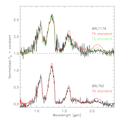
BRLT50: the general shape of the spectrum of this object is well fitted by the T6 standard SDSSp J162414.37+002915.6. However, the peak of the J and H band are slightly lower in the target, and the K band is clearly suppressed, all hints to metal depletion. The kinematics can generally offer insights into the interpretation of the nature of peculiar objects like this one, but with no measured proper motion, we cannot address the possibility of this object belonging to a older disk population.

BRLT179: we assigned a spectral type of T4.5 to this object as the T5 standard reproduces quite well the general shape of the SED in the 0.7 $-$ 1.8 $\mu$ m range, except for the depth of the H₂O absorption at 1.15 and 1.35 $\mu$ m. These features are much better fitted by the T4 standard. The flux level in the K band is extremely suppressed, with almost no flux left. The assigned spectral type is 1 subtype later than the one given in Burningham et al. (2010), but that is based on a 1.05 $-$ 1.35 $\mu$ m spectrum only. The kinematics analysis of BRLT179 performed by Murray et al. (2011) suggests a young disk nature for this object, which is somewhat surprising as BRLT179 is the second bluest T dwarf known (J $-$ K = -1.2 $\pm$ 0.1), and its K band spectrum is strongly suppressed. This apparent inconsistency is in common with the bluest T dwarf known, SDSS J1416+1348B (Burningham et al., 2010; Scholz, 2010) which has young disk kinematics as well.

3.3.3 Low gravity objects

While unusually blue infrared colours are generally tracers of reduced metallicity or high surface gravity, unusually red spectra are the product of an increased metal content or a low surface gravity (which is typical of young objects). We refer the reader to Allers & Liu (2013) and references therein for a more detailed description of the spectral signatures associated (or believed to be associated) with these two atmospheric parameters, and the classification scheme developed for this type of objects.

We identified 2 peculiar low gravity objects within the sample, BRLT22 and BRLT85, and their spectra can be found in Figure 16.

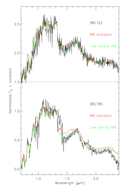
These two late M dwarfs show the peculiar signs of low gravity objects. Specifically they have a somewhat triangular shaped H band, and shallower alkali lines in the J band (in particular in BRLT85). Both objects also show stronger water absorption when compared to the standard template (overplotted in red in Figure 16). In both cases the low gravity M8 template matches better the SED of the target. The gravity classification scheme defined in Allers & Liu (2013) gives a classification of INT-G for BRLT22 and LOW-G for BRLT85, further highlighting the peculiar nature of these two targets. A definitive confirmation has to come from the kinematics, possibly associating the targets to known young moving groups in the solar neighbourhood.

4 Spectral indices and equivalent widths

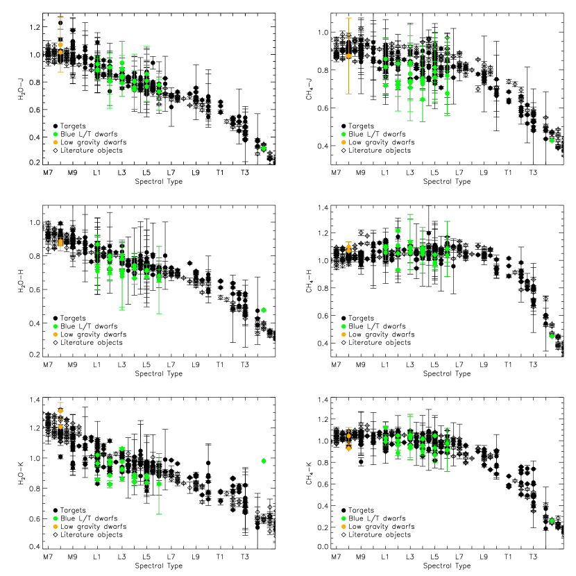
A way to quantify the evolution of spectral features across the spectral sequence is to use spectral indices to measure their strength. The spectral indices calculated for the targets are presented in Table 5, and plotted in Figure 17 and 18. The peculiar objects identified in the previous section are plotted in colour.

In Figure 17 one can see how the indices measuring the relative strength of the water absorption bands (the three plots on the left hand side) correlate very well with spectral types. Blue L dwarfs tend to have stronger water absorption bands and their indices therefore are typical of later type objects (as late as T0 $-$ T1 in some cases), lying below the “main sequence”. A purely index-based classification for these objects could therefore lead to systematically later types.

The right hand side of Figure 17 shows the indices measuring the relative depth of the methane absorption bands. Not surprisingly, the correlation between those indices and spectral type is valid only in the T dwarf range, as there is very little methane absorption in L dwarfs, except at mid-infrared wavelengths.

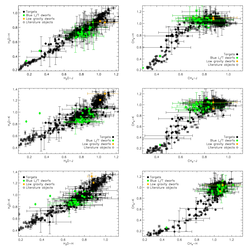
In Figure 18 we present a series of index-index plots. It is easy to spot the “main sequence”, from the late-Ms and early-Ls on the top-right to the mid-Ts in the bottom-left corner of each plot. Once again, the methane indices do not correlate in the L dwarfs regime, with all of the L dwarfs clustered in the 0.8 $-$ 1.0 range for each methane index. When looking at the left hand side of the figure, blue L dwarfs tend to be clustered below the sequence in two of the three plots, further stressing the unusual strength of the $\sim 1.4\mu$ m and the $\sim 1.9\mu$ m water absorption bands, while blue T dwarfs sit above it. In particular the two blue T dwarfs have very high values of the H₂O-K index, which is the effect of their extreme flux suppression in the K band. With very little flux left, their K band spectra are almost flat, and their corresponding indices tend to one.

While these indices give an indication of the evolution of broad molecular absorption bands, to measure the strength of narrow atomic lines we calculated their equivalent width. The main atomic lines in the spectra of brown dwarfs are due to Na i and K i. We calculated the equivalent width of the Na i doublet at 1.139 $\mu$ m, and the K i lines at 1.169, 1.177, 1.244, and 1.253 $\mu$ m, as these are the strongest and best detected lines.

To measure the equivalent width, we fit each doublet and the region of the spectrum around it using a double Gaussian profile. We decided to fit the doublets together since the lines are too close to allow for a separate fit, as one would have to restrict the region to fit too much, leading to a more uncertain determination of the continuum. The continuum is a parameter of the fit, and is assumed to be changing linearly as a function of wavelength. This is to take into account that, especially in late type objects, some of the lines considered do not fall in regions of flat continuum. The centre of the lines is also a parameter of the fit, but the separation between them is fixed and assumed to be equal to the tabulated separation. The equation describing each doublet is therefore:

F(\lambda)=F_{0}+\lambda\times C+a_{1}e^{(\lambda-\lambda_{1})^{2}/2\sigma_{1}^{2}}+a_{2}e^{(\lambda-(\lambda_{1}+\Delta\lambda))^{2}/2\sigma_{2}^{2}}

(1)

where $F_{0}$ and $C$ are the two parameters describing the continuum, $\lambda_{1}$ is the centre of the first line in the doublet, $\Delta\lambda$ is the separation between the two lines, $\sigma_{1}$ and $\sigma_{2}$ are the width of the two lines, and $a_{1}$ and $a_{2}$ are the depth of the two lines, i.e. the minimum flux at the centre of the lines. $F_{0},C,\lambda_{1},a_{1},a_{2},\sigma_{1}$ and $\sigma_{2}$ are all parameters of the fit.

The equivalent width measured for the targets are presented in Table 6 and plotted as a function of effective temperature in Figure 19. Since the Na i doublet at 1.139 $\mu$ m is partly blended, the values presented are the total equivalent width of the doublet. The effective temperature of an object was determined from its spectral type using the type-to-temperature conversion presented in Marocco et al. (2013). Objects with very low signal to noise, or with dubious detection of the lines have been omitted. Measurements with relative errors larger than 0.33 are plotted as open circles, while those with relative errors better than 0.33 are plotted as filled circles. Overplotted for reference are the equivalent width calculated for the BT-Settl atmospheric models (Allard, Homeier, & Freytag, 2011) for solar metallicity, and three different values of surface gravity. The median equivalent width as a function of effective temperature is plotted as a dashed black line, while one standard deviation around it is shown as a grey shaded area. The median is calculated by binning up our targets in 100 K wide bins. The equivalent widths show a large scatter, and there is no clear separation between blue/red L and T dwarfs and the rest of the sample. However, when looking at the median values, our sample appears to be mostly clustered between the log $g$ = 5.0 and log $g$ = 3.5 lines. These values are lower than what one would expect for thin disk objects, i.e. with intermediate ages ( $\approx 1-3$ Gyr). Model isochrones predict values of log $g$ typically around 5 or slightly above (e.g. Allard, Homeier, & Freytag, 2011) for L/T transition dwarfs. The discrepancy could be due to a systematic overestimate of the lines equivalent width in the atmospheric models, possibly due to uncertainties in the measured oscillator strengths in the near-infrared regime (e.g. Table 2, Jones et al., 1996).

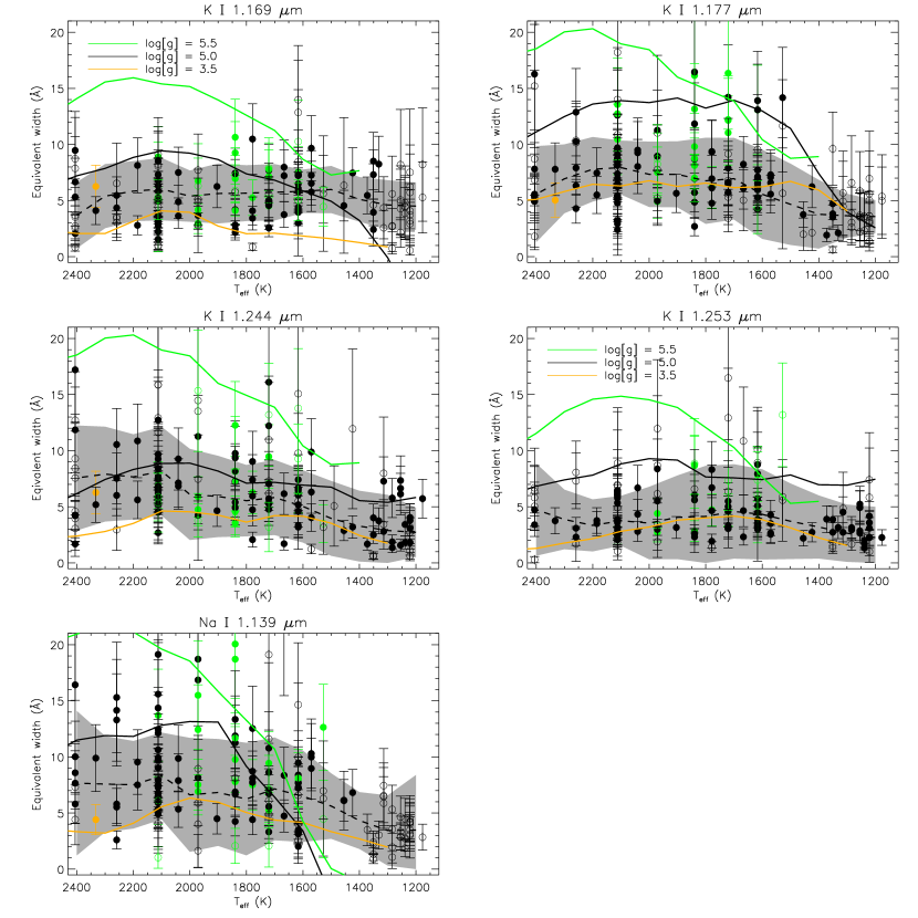
The models suggest that the lines should reach their maximum strength at $T_{\rm eff}\sim 2000$ K, and then slowly get weaker towards lower temperature. Looking at the values from the sample, only the K i lines at 1.244 and 1.253 $\mu$ m follow the expected trend, while the Na i doublet and the K i lines at 1.169 and 1.177 $\mu$ m remain strong even at temperatures as low as $\sim$ 1200 K. However the discrepant measurements tend to have very large associated errors. This is because the mentioned lines fall in regions of growing H₂O and CH₄ absorption, so in late type (i.e. low $T_{\rm eff}$ ) objects the signal-to-noise ratio in those areas decreases sharply, and the fit to the doublet gets less reliable. This would not be a problem in the atmospheric models, nor for the K i lines at 1.244 and 1.253 $\mu$ m since they fall in a region where water and methane absorption is less prominent, and therefore follow the expected trend.

Table 5: Spectral indices for the objects in the sample. For the indices definition, see Table 2.

Name	Spectral type	H₂O-J	H₂O-H	H₂O-K	CH₄-J	CH₄-H	CH₄-K	K/J	H-dip
BRLT28	L6.0 $\pm$ 0.5	0.72	0.69	0.88	0.79	1.04	0.91	0.62	0.48
BRLT49	M9.0 $\pm$ 0.5	0.99	0.87	1.09	0.86	1.00	1.06	0.36	0.49
BRLT63	L1.0 $\pm$ 0.5	0.97	0.82	1.11	0.87	1.01	0.98	0.41	0.49
BRLT65	M9.0 $\pm$ 0.5	0.99	0.90	1.09	0.87	1.00	1.07	0.37	0.49
BRLT67	L1.0 $\pm$ 0.5	0.97	0.81	1.01	0.88	1.06	1.05	0.39	0.48
BRLT68	L5.0 $\pm$ 0.5	0.82	0.70	0.88	0.82	1.04	0.92	0.64	0.51
BRLT69	L1.0 $\pm$ 0.5	0.95	0.86	1.08	0.92	1.04	1.07	0.41	0.48
BRLT71	L1.5 $\pm$ 0.5	0.96	0.80	1.06	0.89	1.00	0.97	0.43	0.49
BRLT72	M9.0 $\pm$ 0.5	1.05	0.91	1.13	0.90	1.04	1.07	0.39	0.49
BRLT73	L1.0 $\pm$ 0.5	0.93	0.85	0.99	0.84	1.12	0.92	0.44	0.50
BRLT74	L9.5 $\pm$ 1.0	0.67	0.66	0.76	0.70	1.03	0.73	0.50	0.53
BRLT75	M9.0 $\pm$ 1.0	1.00	0.89	1.14	0.91	1.04	1.04	0.34	0.49
BRLT76	L5.5 $\pm$ 0.5	0.78	0.81	0.97	0.82	1.08	0.96	0.57	0.49
BRLT78	L1.0 $\pm$ 0.5	0.98	0.84	1.11	0.80	1.07	1.04	0.35	0.51
BRLT81	M9.0 $\pm$ 0.5	1.07	0.88	1.07	0.89	1.01	0.99	0.41	0.49
BRLT82	L1.0 $\pm$ 0.5	0.94	0.85	1.07	0.88	1.05	1.02	0.43	0.49
BRLT83	M8.0 $\pm$ 1.0	1.11	0.99	1.32	0.94	1.02	0.94	0.37	0.49
BRLT84	L3.5 $\pm$ 0.5	0.77	0.77	0.95	0.81	1.06	1.03	0.49	0.49
BRLT85	M8.0 $\pm$ 0.5	1.07	0.87	1.31	0.87	1.10	1.04	0.28	0.50
BRLT87	T0.0 $\pm$ 0.5	0.59	0.58	0.77	0.66	0.90	0.69	0.41	0.48
BRLT88	L4.0 $\pm$ 1.0	0.83	0.78	1.01	0.83	1.06	1.06	0.50	0.48
BRLT91	T3.0 $\pm$ 0.5	0.47	0.46	0.68	0.53	0.79	0.49	0.25	0.47
BRLT92	L1.0 $\pm$ 0.5	0.86	0.83	1.00	0.82	1.08	1.02	0.39	0.48
BRLT97	L0.0 $\pm$ 1.0	0.99	0.84	1.13	0.92	1.03	0.98	0.39	0.49
BRLT99	L5.0 $\pm$ 0.5	0.81	0.71	0.85	0.84	1.08	0.98	0.55	0.48
BRLT101	L3.0 $\pm$ 1.0	0.83	0.68	0.86	0.73	1.13	1.02	0.34	0.49
BRLT102	L0.0 $\pm$ 0.5	0.94	0.88	1.06	0.91	1.03	1.05	0.42	0.49
BRLT103	L5.5 $\pm$ 0.5	0.74	0.74	0.92	0.71	1.00	0.89	0.36	0.50
BRLT104	M9.0 $\pm$ 0.5	1.08	0.93	0.93	0.96	0.98	0.80	0.40	0.46
BRLT105	L5.0 $\pm$ 0.5	0.82	0.78	0.96	0.84	1.07	0.99	0.53	0.48
BRLT106	M9.0 $\pm$ 0.5	0.97	0.88	0.97	0.84	1.03	1.00	0.37	0.48
BRLT108	L6.5 $\pm$ 0.5	0.79	0.73	0.91	0.82	1.10	1.01	0.68	0.47
BRLT111	L2.0 $\pm$ 0.5	0.86	0.77	0.90	0.81	1.05	1.06	0.53	0.48
BRLT112	L1.0 $\pm$ 0.5	0.86	0.79	0.98	0.85	1.04	0.95	0.43	0.48
BRLT113	M9.0 $\pm$ 0.5	1.17	0.88	1.05	0.93	1.02	1.05	0.36	0.47
BRLT114	L6.0 $\pm$ 0.5	0.76	0.73	0.91	0.82	1.08	0.93	0.68	0.52
BRLT116	T2.5 $\pm$ 0.5	0.55	0.54	0.82	0.62	0.85	0.74	0.33	0.46
BRLT117	L5.0 $\pm$ 1.0	0.88	0.70	0.81	0.78	1.03	0.89	0.56	0.48
BRLT119	L4.0 $\pm$ 0.5	0.87	0.76	0.90	0.86	1.03	1.01	0.51	0.46
BRLT121	L1.0 $\pm$ 0.5	0.91	0.80	0.99	0.81	1.01	1.03	0.36	0.47
BRLT122	L1.0 $\pm$ 0.5	0.91	0.84	0.95	0.82	1.04	0.90	0.40	0.50
BRLT123	L2.0 $\pm$ 0.5	0.95	0.80	0.94	0.85	1.03	1.05	0.47	0.46
BRLT129	L5.0 $\pm$ 1.0	0.80	0.70	0.95	0.79	1.04	0.95	0.58	0.49
BRLT130	L3.0 $\pm$ 1.0	0.94	0.69	0.93	0.78	1.10	1.04	0.34	0.49
BRLT133	M9.0 $\pm$ 0.5	1.04	0.86	0.96	0.91	0.99	0.98	0.42	0.46
BRLT136	L1.0 $\pm$ 1.0	0.93	0.87	0.96	0.86	1.06	1.02	0.37	0.48
BRLT137	L4.5 $\pm$ 0.5	0.76	0.72	0.88	0.75	1.04	0.91	0.52	0.50
BRLT138	L2.0 $\pm$ 1.0	0.88	0.82	0.97	0.86	1.06	0.98	0.50	0.49
BRLT139	L4.0 $\pm$ 1.0	0.80	0.74	0.84	0.73	1.04	0.95	0.41	0.49
BRLT140	L0.0 $\pm$ 0.5	0.94	0.86	0.96	0.84	1.07	1.00	0.41	0.48
BRLT142	L2.5 $\pm$ 0.5	0.85	0.82	0.97	0.85	1.08	0.98	0.54	0.49
BRLT144	L5.0 $\pm$ 1.0	0.86	0.68	0.84	0.81	0.97	0.93	0.46	0.47
BRLT145	L1.0 $\pm$ 0.5	0.93	0.83	1.01	0.84	1.02	0.99	0.42	0.49
BRLT149	L6.0 $\pm$ 1.0	0.78	0.68	0.83	0.77	1.04	0.98	0.43	0.49
BRLT152	L0.0 $\pm$ 0.5	1.05	0.91	0.99	0.91	1.03	1.03	0.41	0.49
BRLT153	L1.0 $\pm$ 0.5	0.91	0.84	1.02	0.82	1.06	1.02	0.34	0.48
BRLT155	L3.0 $\pm$ 1.0	0.86	0.75	1.05	0.88	1.09	1.00	0.50	0.49
BRLT159	L9.0 $\pm$ 0.5	0.73	0.67	0.80	0.78	1.02	0.89	0.62	0.50
BRLT162	L0.5 $\pm$ 0.5	0.97	0.86	1.11	0.84	1.06	1.06	0.35	0.49
BRLT163	L1.0 $\pm$ 0.5	0.83	0.83	1.02	0.90	1.05	1.09	0.44	0.48
BRLT164	T3.0 $\pm$ 0.5	0.54	0.53	0.71	0.57	0.70	0.39	0.24	0.46
BRLT165	L2.0 $\pm$ 0.5	0.92	0.86	0.95	0.90	1.04	1.03	0.46	0.50
BRLT168	L4.0 $\pm$ 0.5	0.79	0.75	0.92	0.80	1.09	1.03	0.56	0.46
BRLT171	L5.0 $\pm$ 0.5	0.79	0.74	0.94	0.82	1.08	1.00	0.55	0.49
BRLT176	L4.0 $\pm$ 1.0	0.87	0.77	0.96	0.79	1.01	0.96	0.44	0.49
BRLT181	L1.0 $\pm$ 1.0	1.09	0.88	1.09	0.89	1.03	1.01	0.42	0.49
BRLT182	T3.0 $\pm$ 0.5	0.51	0.50	0.74	0.57	0.79	0.61	0.37	0.44
BRLT186	L1.0 $\pm$ 1.0	0.92	0.85	1.04	0.85	1.04	1.03	0.39	0.49
BRLT190	T4.0 $\pm$ 0.5	0.34	0.47	0.54	0.48	0.54	0.19	0.22	0.36
BRLT197	T2.0 $\pm$ 1.0	0.54	0.64	0.87	0.66	0.88	0.70	0.44	0.47
BRLT198	L3.0 $\pm$ 1.0	0.90	0.80	1.06	0.84	1.06	1.04	0.39	0.47
BRLT202	T2.5 $\pm$ 0.5	0.45	0.57	0.81	0.52	0.79	0.60	0.32	0.44
BRLT203	T3.0 $\pm$ 1.0	0.39	0.58	0.82	0.53	0.81	0.74	0.46	0.44
BRLT206	L2.0 $\pm$ 0.5	0.90	0.83	0.91	0.82	1.06	1.10	0.45	0.48
BRLT210	L4.5 $\pm$ 0.5	0.77	0.75	0.96	0.82	1.09	1.01	0.54	0.49
BRLT216	M9.0 $\pm$ 0.5	1.10	0.88	1.07	0.90	1.00	0.99	0.39	0.49
BRLT217	T0.0 $\pm$ 0.5	0.69	0.66	0.89	0.75	0.94	0.78	0.50	0.52
BRLT218	L6.0 $\pm$ 0.5	0.79	0.71	0.95	0.80	1.13	1.04	0.62	0.52
BRLT219	T3.0 $\pm$ 0.5	0.43	0.46	0.73	0.52	0.68	0.40	0.26	0.44
BRLT220	L2.0 $\pm$ 0.5	0.89	0.77	0.83	0.85	1.09	1.07	0.51	0.47
BRLT227	L3.0 $\pm$ 0.5	0.83	0.76	0.91	0.85	1.10	1.07	0.55	0.50
BRLT229	M8.0 $\pm$ 0.5	1.23	0.95	1.01	0.95	1.05	1.04	0.37	0.50
BRLT231	L5.0 $\pm$ 0.5	0.87	0.77	0.91	0.85	1.07	1.00	0.59	0.49
BRLT234	L4.0 $\pm$ 1.0	0.74	0.67	0.87	0.64	1.09	0.95	0.26	0.50
BRLT236	L3.5 $\pm$ 0.5	0.82	0.71	0.93	0.76	1.07	0.97	0.43	0.49
BRLT237	L4.0 $\pm$ 0.5	0.84	0.69	0.88	0.84	1.09	0.99	0.49	0.51
BRLT240	L3.0 $\pm$ 0.5	0.94	0.82	0.93	0.90	1.05	1.05	0.55	0.47
BRLT243	T0.0 $\pm$ 0.5	0.70	0.60	0.73	0.69	1.01	0.76	0.50	0.51
BRLT247	M9.0 $\pm$ 0.5	1.09	0.90	1.09	0.93	0.97	1.00	0.41	0.48
BRLT249	L5.0 $\pm$ 0.5	0.84	0.71	0.84	0.84	1.05	0.92	0.57	0.50
BRLT250	L1.0 $\pm$ 0.5	0.85	0.77	0.83	0.79	1.05	0.94	0.46	0.49
BRLT251	L1.0 $\pm$ 0.5	0.92	0.80	0.94	0.80	1.00	0.94	0.34	0.48
BRLT253	L1.0 $\pm$ 1.0	0.89	0.71	0.86	0.72	1.09	0.99	0.27	0.48
BRLT254	L5.0 $\pm$ 0.5	0.84	0.82	0.95	0.89	1.06	1.04	0.54	0.49
BRLT260	L2.0 $\pm$ 1.0	0.80	0.70	0.89	0.71	1.11	1.00	0.29	0.49
BRLT262	L0.0 $\pm$ 0.5	0.90	0.82	0.96	0.89	1.12	1.02	0.47	0.49
BRLT265	L2.0 $\pm$ 0.5	0.89	0.80	0.92	0.80	1.04	1.07	0.47	0.48
BRLT269	L7.0 $\pm$ 0.5	0.62	0.69	0.91	0.82	1.10	0.99	0.76	0.50
BRLT270	L2.0 $\pm$ 1.0	0.81	0.72	0.83	0.72	1.05	0.89	0.33	0.50
BRLT274	L2.0 $\pm$ 0.5	0.73	0.76	1.11	0.89	1.17	1.07	0.63	0.48
BRLT276	L0.0 $\pm$ 0.5	0.96	0.83	1.06	0.85	1.02	1.03	0.38	0.49
BRLT279	L1.0 $\pm$ 0.5	0.91	0.83	1.01	0.82	1.05	1.03	0.39	0.48
BRLT283	L5.0 $\pm$ 1.0	0.81	0.71	0.88	0.79	0.99	0.87	0.37	0.49
BRLT285	L5.0 $\pm$ 0.5	0.80	0.73	0.78	0.82	1.05	0.96	0.62	0.52
BRLT290	T2.0 $\pm$ 0.5	0.50	0.49	0.78	0.58	0.90	0.61	0.35	0.50
BRLT295	L4.0 $\pm$ 2.0	0.83	0.80	0.99	0.76	0.96	0.97	0.33	0.47
BRLT296	L4.0 $\pm$ 0.5	0.84	0.75	0.89	0.82	1.05	0.99	0.46	0.49
BRLT297	L4.5 $\pm$ 0.5	0.83	0.76	0.95	0.89	1.06	1.00	0.52	0.50
BRLT299	L4.0 $\pm$ 1.0	0.77	0.74	0.90	0.76	1.03	0.92	0.46	0.49
BRLT301	L1.0 $\pm$ 0.5	0.92	0.77	0.92	0.82	1.03	1.03	0.42	0.47
BRLT302	L4.0 $\pm$ 1.0	0.81	0.72	0.89	0.76	1.07	0.90	0.39	0.49
BRLT308	L5.0 $\pm$ 0.5	0.74	0.72	0.94	0.82	1.09	1.03	0.57	0.50
BRLT319	T3.0 $\pm$ 0.5	0.42	0.47	0.69	0.50	0.79	0.43	0.28	0.47
BRLT340	L4.0 $\pm$ 0.5	0.79	0.75	0.97	0.90	1.08	1.06	0.49	0.49

Table 6: The equivalent width obtained from the spectra. Missing entries indicate the non detection of the line, due either to the line being too weak or the spectrum being too noisy. Numbers in italics indicate measurements with relative errors larger than 0.33. For the details on how these values were calculated, see Section 4.

		Equivalent width (Å)
Name	Spectral type	Na i	K i	K i	K i	K i
		1.139 $\mu$ m	1.169 $\mu$ m	1.177 $\mu$ m	1.244 $\mu$ m	1.253 $\mu$ m
BRLT1	L9.0 $\pm$ 0.5	0.90	8.52	3.83	2.50	2.73
BRLT2	L1.0 $\pm$ 1.0	6.79	5.23	4.77	9.27	2.38
BRLT3	L9.0 $\pm$ 1.0	1.33	3.95	4.72	0.57	3.87
BRLT6	L3.0 $\pm$ 1.0	6.88	2.15	2.70	9.36	2.58
BRLT7	M8.0 $\pm$ 1.0	6.41	1.26	5.69	3.04	4.95
BRLT8	L8.5 $\pm$ 0.5	3.50	5.46	1.92	1.68	3.89
BRLT9	L1.0 $\pm$ 1.0	7.38	4.97	8.39	5.20	6.09
BRLT10	L9.0 $\pm$ 0.5	2.41	2.42	3.52	0.67	1.32
BRLT12	L3.0 $\pm$ 1.0	4.24	2.82	8.70	5.39	5.61
BRLT14	L0.0 $\pm$ 0.5	$\ldots$	$\ldots$	$\ldots$	$\ldots$	$\ldots$
BRLT15	T2.0 $\pm$ 2.0	$\ldots$	4.29	2.20	1.57	2.66
BRLT16	L2.0 $\pm$ 1.0	6.92	6.76	4.91	5.89	2.72
BRLT18	L0.0 $\pm$ 1.0	$\ldots$	$\ldots$	$\ldots$	$\ldots$	$\ldots$
BRLT20	L1.0 $\pm$ 1.0	5.90	5.08	8.69	5.77	2.06
BRLT21	L3.5 $\pm$ 0.5	8.09	4.08	9.37	7.41	8.32
BRLT22	M8.0 $\pm$ 0.5	4.41	6.26	5.04	6.27	$\ldots$
BRLT24	L3.5 $\pm$ 0.5	12.53	3.42	6.94	5.96	6.70
BRLT26	L5.5 $\pm$ 0.5	8.97	5.77	5.57	4.03	2.66
BRLT27	T0.0 $\pm$ 0.5	3.55	5.59	3.87	5.78	1.67
BRLT28	L6.0 $\pm$ 0.5	$\ldots$	5.62	5.65	$\ldots$	$\ldots$
BRLT30	L5.0 $\pm$ 0.5	$\ldots$	$\ldots$	$\ldots$	4.72	$\ldots$
BRLT31	L4.0 $\pm$ 1.0	3.32	4.61	6.50	5.72	4.59
BRLT32	L1.5 $\pm$ 0.5	7.89	3.63	9.26	9.26	6.69
BRLT33	L3.5 $\pm$ 0.5	4.41	0.87	9.33	9.04	4.65
BRLT35	M9.5 $\pm$ 0.5	9.89	4.11	7.79	5.19	3.75
BRLT37	L5.0 $\pm$ 0.5	8.38	3.00	6.83	6.46	5.72
BRLT38	T0.0 $\pm$ 0.5	5.33	2.69	3.04	1.36	2.95
BRLT39	L5.0 $\pm$ 1.0	3.29	6.08	7.12	5.18	7.94
BRLT42	M9.0 $\pm$ 0.5	8.58	0.81	5.57	1.68	3.40
BRLT44	L5.0 $\pm$ 1.0	2.02	7.24	7.71	3.34	3.00
BRLT45	T1.0 $\pm$ 0.5	1.07	0.73	2.63	1.88	3.14
BRLT46	L0.5 $\pm$ 0.5	9.54	8.13	7.45	10.87	3.50
BRLT48	L4.5 $\pm$ 0.5	$\ldots$	$\ldots$	$\ldots$	$\ldots$	$\ldots$
BRLT49	M9.0 $\pm$ 0.5	$\ldots$	2.72	5.23	3.95	5.04
BRLT50	T6.0 $\pm$ 0.5	$\ldots$	$\ldots$	$\ldots$	$\ldots$	$\ldots$
BRLT51	L3.0 $\pm$ 1.0	11.88	4.20	4.86	9.75	2.31
BRLT52	L5.5 $\pm$ 0.5	$\ldots$	6.53	7.08	1.24	3.51
BRLT56	L1.5 $\pm$ 1.0	5.34	4.89	9.50	7.13	4.33
BRLT57	L0.0 $\pm$ 1.0	5.53	4.35	4.29	7.53	3.09
BRLT58	L4.0 $\pm$ 1.0	5.26	4.51	11.05	9.47	4.71
BRLT60	L1.0 $\pm$ 1.0	12.12	5.83	2.94	9.67	2.43
BRLT62	L5.0 $\pm$ 1.0	9.46	4.39	6.54	7.42	3.37
BRLT63	L1.0 $\pm$ 0.5	6.03	3.11	5.03	6.67	6.96
BRLT64	L4.0 $\pm$ 0.5	10.78	2.56	6.51	$\ldots$	5.02
BRLT65	M9.0 $\pm$ 0.5	$\ldots$	$\ldots$	5.44	4.58	5.82
BRLT66	L5.0 $\pm$ 0.5	7.67	3.95	5.28	6.04	4.49
BRLT67	L1.0 $\pm$ 0.5	8.17	4.98	3.20	7.99	8.89
BRLT68	L5.0 $\pm$ 0.5	14.65	4.99	$\ldots$	$\ldots$	3.22
BRLT69	L1.0 $\pm$ 0.5	9.03	2.97	5.19	5.65	5.35
BRLT71	L1.5 $\pm$ 0.5	9.86	7.50	8.03	6.84	2.80
BRLT72	M9.0 $\pm$ 0.5	7.66	2.06	7.81	4.20	4.75
BRLT73	L1.0 $\pm$ 0.5	9.70	6.78	9.71	12.73	6.47
BRLT74	L9.5 $\pm$ 1.0	3.04	8.25	2.12	3.74	3.16
BRLT75	M9.0 $\pm$ 1.0	5.80	5.32	4.95	4.26	0.29
BRLT76	L5.5 $\pm$ 0.5	9.98	7.26	6.58	9.89	2.55
BRLT78	L1.0 $\pm$ 0.5	15.59	8.53	14.00	8.82	$\ldots$
BRLT81	M9.0 $\pm$ 0.5	4.43	2.52	4.94	7.57	$\ldots$
BRLT82	L1.0 $\pm$ 0.5	7.93	3.65	7.38	7.66	3.86
BRLT83	M8.0 $\pm$ 1.0	7.97	6.65	5.46	5.51	5.07
BRLT84	L3.5 $\pm$ 0.5	7.73	$\ldots$	4.77	2.07	1.93
BRLT85	M8.0 $\pm$ 0.5	5.84	5.77	4.03	5.36	$\ldots$
BRLT87	T0.0 $\pm$ 0.5	1.96	2.74	6.58	$\ldots$	$\ldots$
BRLT88	L4.0 $\pm$ 1.0	5.57	7.69	7.89	4.77	3.30
BRLT91	T3.0 $\pm$ 0.5	4.00	6.22	2.96	0.62	4.17
BRLT92	L1.0 $\pm$ 0.5	6.48	3.16	6.49	7.47	3.77
BRLT97	L0.0 $\pm$ 1.0	2.60	5.46	6.33	6.02	2.30
BRLT98	T4.0 $\pm$ 0.5	$\ldots$	8.21	5.37	$\ldots$	$\ldots$
BRLT99	L5.0 $\pm$ 0.5	$\ldots$	8.47	6.21	5.50	$\ldots$
BRLT101	L3.0 $\pm$ 0.5	18.71	7.25	13.16	12.27	$\ldots$
BRLT102	L0.0 $\pm$ 0.5	14.15	6.53	12.87	$\ldots$	$\ldots$
BRLT103	L5.5 $\pm$ 0.5	10.30	9.66	7.30	6.31	4.27
BRLT104	M9.0 $\pm$ 0.5	21.60	9.47	1.81	12.72	6.38
BRLT105	L5.0 $\pm$ 0.5	7.70	6.49	6.97	6.64	3.53
BRLT106	M9.0 $\pm$ 0.5	7.32	8.73	8.72	17.21	$\ldots$
BRLT108	L6.5 $\pm$ 0.5	$\ldots$	$\ldots$	2.14	11.95	$\ldots$
BRLT111	L2.0 $\pm$ 0.5	5.89	5.12	11.27	$\ldots$	11.96
BRLT112	L1.0 $\pm$ 0.5	6.48	$\ldots$	9.63	15.86	4.92
BRLT113	M9.0 $\pm$ 0.5	$\ldots$	7.86	15.20	11.86	6.69
BRLT114	L6.0 $\pm$ 0.5	6.29	$\ldots$	14.17	$\ldots$	5.59
BRLT116	T2.5 $\pm$ 0.5	$\ldots$	4.81	$\ldots$	$\ldots$	$\ldots$
BRLT117	L5.0 $\pm$ 0.5	2.56	13.99	13.90	9.77	8.93
BRLT119	L4.0 $\pm$ 0.5	19.11	5.58	5.31	10.97	16.48
BRLT121	L1.0 $\pm$ 0.5	29.10	8.06	12.60	8.68	$\ldots$
BRLT122	L1.0 $\pm$ 0.5	10.63	4.97	9.10	6.53	1.04
BRLT123	L2.0 $\pm$ 0.5	18.71	$\ldots$	11.03	$\ldots$	1.89
BRLT129	L5.0 $\pm$ 1.0	3.13	7.27	6.11	3.19	3.86
BRLT130	L3.0 $\pm$ 0.5	20.06	10.64	8.77	3.99	$\ldots$
BRLT131	T3.0 $\pm$ 0.5	4.47	4.07	3.07	3.79	3.09
BRLT133	M9.0 $\pm$ 0.5	10.02	3.52	5.27	8.43	$\ldots$
BRLT135	T2.5 $\pm$ 0.5	1.87	3.86	3.57	$\ldots$	1.32
BRLT136	L1.0 $\pm$ 1.0	6.10	5.32	12.74	5.37	$\ldots$
BRLT137	L4.5 $\pm$ 0.5	8.36	7.98	6.09	1.71	4.66
BRLT138	L2.0 $\pm$ 1.0	8.16	3.67	4.97	4.23	2.98
BRLT139	L5.0 $\pm$ 0.5	7.14	7.92	12.15	13.20	7.34
BRLT140	L0.0 $\pm$ 0.5	15.30	3.56	10.37	$\ldots$	1.69
BRLT142	L2.5 $\pm$ 0.5	4.49	6.25	5.65	4.64	3.15
BRLT144	L5.0 $\pm$ 0.5	$\ldots$	10.26	4.40	13.78	6.10
BRLT145	L1.0 $\pm$ 0.5	7.44	5.15	9.39	15.89	$\ldots$
BRLT147	T3.0 $\pm$ 0.5	$\ldots$	5.72	5.02	1.82	2.28
BRLT149	L6.0 $\pm$ 0.5	12.64	4.46	$\ldots$	$\ldots$	13.19
BRLT152	L0.0 $\pm$ 0.5	13.29	3.42	10.16	$\ldots$	8.06
BRLT153	L1.0 $\pm$ 0.5	3.69	3.85	10.86	12.93	$\ldots$
BRLT155	L3.0 $\pm$ 1.0	11.26	2.45	5.72	8.17	$\ldots$
BRLT159	L9.0 $\pm$ 0.5	$\ldots$	4.61	9.62	$\ldots$	$\ldots$
BRLT162	L0.5 $\pm$ 0.5	7.51	2.79	5.51	5.62	3.77
BRLT163	L1.0 $\pm$ 0.5	19.13	5.04	5.45	7.36	6.29
BRLT164	T3.0 $\pm$ 0.5	3.14	$\ldots$	6.96	2.72	$\ldots$
BRLT165	L2.0 $\pm$ 0.5	1.63	$\ldots$	$\ldots$	14.47	5.52
BRLT168	L4.0 $\pm$ 0.5	6.73	4.78	9.16	12.21	12.93
BRLT171	L5.0 $\pm$ 0.5	7.22	5.79	5.95	4.61	3.26
BRLT176	L4.0 $\pm$ 1.0	$\ldots$	$\ldots$	$\ldots$	$\ldots$	$\ldots$
BRLT179	T4.5 $\pm$ 0.5	$\ldots$	$\ldots$	$\ldots$	$\ldots$	$\ldots$
BRLT181	L1.0 $\pm$ 1.0	7.28	7.31	6.98	4.58	3.60
BRLT182	T3.0 $\pm$ 0.5	3.02	2.93	5.61	3.18	7.41
BRLT186	L1.0 $\pm$ 1.0	7.48	2.24	5.39	4.51	2.92
BRLT190	T4.0 $\pm$ 0.5	$\ldots$	$\ldots$	$\ldots$	$\ldots$	$\ldots$
BRLT197	T2.0 $\pm$ 1.0	2.84	4.87	3.53	6.65	2.85
BRLT198	L3.0 $\pm$ 0.5	2.07	5.90	16.15	8.15	8.87
BRLT202	T2.5 $\pm$ 0.5	4.49	4.41	3.57	1.82	2.02
BRLT203	T3.0 $\pm$ 1.0	4.15	3.20	3.63	4.05	1.01
BRLT206	L2.0 $\pm$ 0.5	16.86	4.89	8.94	7.47	3.43
BRLT207	L7.0 $\pm$ 0.5	6.14	4.55	3.75	2.88	2.19
BRLT210	L4.5 $\pm$ 0.5	4.74	3.75	8.24	6.16	2.32
BRLT212	L6.0 $\pm$ 2.0	4.46	$\ldots$	$\ldots$	3.52	$\ldots$
BRLT216	M9.0 $\pm$ 0.5	$\ldots$	6.66	6.84	3.07	$\ldots$
BRLT217	T0.0 $\pm$ 0.5	$\ldots$	$\ldots$	4.93	3.43	$\ldots$
BRLT218	L6.0 $\pm$ 0.5	6.97	6.01	11.66	3.17	5.89
BRLT219	T3.0 $\pm$ 0.5	$\ldots$	$\ldots$	$\ldots$	$\ldots$	$\ldots$
BRLT220	L2.0 $\pm$ 0.5	4.01	7.71	7.76	$\ldots$	8.67
BRLT227	L3.0 $\pm$ 0.5	8.12	5.75	16.46	7.24	6.59
BRLT229	M8.0 $\pm$ 0.5	5.02	$\ldots$	11.39	4.85	2.87
BRLT231	L5.0 $\pm$ 0.5	6.58	12.85	9.54	15.08	10.09
BRLT232	T2.5 $\pm$ 0.5	2.74	4.51	2.32	3.42	1.71
BRLT234	L4.0 $\pm$ 1.0	9.44	7.80	12.22	7.10	4.57
BRLT236	L3.5 $\pm$ 0.5	$\ldots$	$\ldots$	$\ldots$	$\ldots$	$\ldots$
BRLT237	L4.0 $\pm$ 0.5	6.12	4.88	14.21	6.18	$\ldots$
BRLT240	L3.0 $\pm$ 0.5	13.35	7.40	11.84	$\ldots$	2.69
BRLT243	T0.0 $\pm$ 0.5	6.55	$\ldots$	$\ldots$	7.99	4.86
BRLT247	M9.0 $\pm$ 0.5	16.42	3.70	16.27	9.29	$\ldots$
BRLT249	L5.0 $\pm$ 0.5	4.02	7.47	$\ldots$	$\ldots$	$\ldots$
BRLT250	L1.0 $\pm$ 0.5	5.99	9.14	8.69	6.73	6.40
BRLT251	L1.0 $\pm$ 0.5	4.05	$\ldots$	3.27	$\ldots$	6.88
BRLT253	L1.0 $\pm$ 0.5	1.03	5.08	13.56	5.89	$\ldots$
BRLT254	L5.0 $\pm$ 0.5	9.96	$\ldots$	13.09	$\ldots$	$\ldots$
BRLT258	L5.0 $\pm$ 1.0	$\ldots$	$\ldots$	$\ldots$	$\ldots$	$\ldots$
BRLT260	L2.0 $\pm$ 0.5	15.49	4.18	8.72	3.77	$\ldots$
BRLT262	L0.0 $\pm$ 0.5	5.80	3.06	10.26	10.55	7.30
BRLT265	L2.0 $\pm$ 0.5	8.94	2.86	8.95	11.27	8.38
BRLT269	L7.0 $\pm$ 0.5	14.63	$\ldots$	5.99	7.25	$\ldots$
BRLT270	L2.0 $\pm$ 0.5	12.43	6.30	8.25	15.34	$\ldots$
BRLT274	L2.0 $\pm$ 0.5	$\ldots$	2.74	5.22	13.52	6.16
BRLT275	T2.0 $\pm$ 2.0	4.64	2.16	3.69	6.13	4.94
BRLT276	L0.0 $\pm$ 0.5	$\ldots$	$\ldots$	7.91	2.96	$\ldots$
BRLT279	L1.0 $\pm$ 0.5	8.03	4.44	7.97	5.10	$\ldots$
BRLT281	T0.0 $\pm$ 1.0	7.44	$\ldots$	5.68	$\ldots$	$\ldots$
BRLT283	L5.0 $\pm$ 0.5	8.11	5.03	13.08	9.28	7.37
BRLT285	L5.0 $\pm$ 0.5	3.25	7.24	$\ldots$	$\ldots$	8.77
BRLT287	T3.0 $\pm$ 0.5	3.48	3.73	3.63	3.09	3.58
BRLT290	T2.0 $\pm$ 0.5	10.65	3.05	5.31	$\ldots$	$\ldots$
BRLT295	L4.0 $\pm$ 2.0	$\ldots$	$\ldots$	$\ldots$	5.07	$\ldots$
BRLT296	L4.0 $\pm$ 0.5	4.88	4.97	3.42	16.10	3.07
BRLT297	L4.5 $\pm$ 0.5	22.31	7.22	5.03	$\ldots$	10.87
BRLT299	L4.0 $\pm$ 1.0	7.06	5.02	5.73	5.28	3.10
BRLT301	L1.0 $\pm$ 0.5	9.14	8.24	18.21	11.62	$\ldots$
BRLT302	L4.0 $\pm$ 0.5	2.08	7.14	16.35	3.20	$\ldots$
BRLT305	L5.5 $\pm$ 1.0	$\ldots$	$\ldots$	$\ldots$	$\ldots$	$\ldots$
BRLT306	L4.5 $\pm$ 1.0	$\ldots$	$\ldots$	$\ldots$	$\ldots$	$\ldots$
BRLT307	L1.0 $\pm$ 0.5	9.93	0.99	2.40	8.40	3.16
BRLT308	L5.0 $\pm$ 0.5	7.27	$\ldots$	5.15	$\ldots$	$\ldots$
BRLT309	L7.0 $\pm$ 0.5	6.11	6.35	2.00	$\ldots$	$\ldots$
BRLT311	T3.0 $\pm$ 0.5	4.25	0.55	1.36	1.09	2.25
BRLT312	T0.0 $\pm$ 0.5	6.46	2.57	4.47	7.28	4.52
BRLT313	L3.5 $\pm$ 0.5	8.72	10.48	6.12	4.73	1.41
BRLT314	L7.5 $\pm$ 0.5	6.82	7.46	6.24	3.20	2.73
BRLT315	L1.0 $\pm$ 1.0	5.33	1.56	8.78	6.81	5.95
BRLT316	L1.0 $\pm$ 0.5	12.46	2.74	3.19	2.69	5.79
BRLT317	L3.0 $\pm$ 1.0	9.77	6.95	9.81	4.57	8.67
BRLT318	L1.0 $\pm$ 0.5	14.36	6.33	6.22	6.20	6.10
BRLT319	T3.0 $\pm$ 0.5	4.19	7.52	3.21	$\ldots$	5.84
BRLT320	L1.0 $\pm$ 0.5	4.90	0.90	8.12	6.34	1.88
BRLT321	T4.0 $\pm$ 0.5	2.85	5.28	4.99	5.73	2.26
BRLT322	L5.0 $\pm$ 0.5	3.48	4.19	4.20	6.66	5.10
BRLT323	L5.0 $\pm$ 1.0	7.97	7.54	6.30	6.35	7.85
BRLT325	T2.0 $\pm$ 1.0	3.35	8.20	5.85	7.34	4.93
BRLT328	L3.0 $\pm$ 1.0	7.78	9.25	8.12	7.30	2.85
BRLT330	L2.0 $\pm$ 1.0	7.53	2.97	7.51	4.76	4.40
BRLT331	L3.0 $\pm$ 1.0	11.68	4.10	7.02	3.56	8.74
BRLT332	L2.0 $\pm$ 1.0	6.67	7.44	6.96	4.92	6.05
BRLT333	T2.0 $\pm$ 0.5	2.92	5.06	3.55	$\ldots$	5.24
BRLT334	L3.5 $\pm$ 0.5	7.51	5.26	6.19	6.27	4.74
BRLT335	L4.0 $\pm$ 1.0	8.62	4.56	6.62	7.05	5.50
BRLT338	L1.0 $\pm$ 1.0	13.70	8.90	10.46	6.94	2.44
BRLT340	L4.0 $\pm$ 0.5	11.60	$\ldots$	6.78	7.30	6.37
BRLT343	L9.0 $\pm$ 1.0	2.24	7.31	0.62	4.02	1.53
BRLT344	T0.0 $\pm$ 1.0	5.87	4.36	$\ldots$	2.80	2.73

5 Radial velocities

Using a cross-correlation technique we calculated the radial velocities for the objects in the sample. An example of a cross-correlation function (hereafter CCF) obtained is shown in Figure 20. The CCF shows a clear sharp peak around -1 pix, highlighting the precision of the radial velocity obtained. The exact position of the CCF peak was determined using the procedure described in Taylor (1992) and Press, Flannery, & Teukolsky (1986). The two main telluric bands at 1.35 $-$ 1.45 $\mu$ m and 1.80 $-$ 1.95 $\mu$ m are not considered when evaluating the CCF, to avoid a possible systematic bias towards smaller velocities.

The radial velocities have been measured relative to Kelu-1, for which we obtained a very high signal-to-noise ratio spectrum on the night of 07-04-2013. The radial velocity of Kelu-1 is given in Blake, Charbonneau, & White (2010) and is 6.37 $\pm$ 0.35 km s^-1. Kelu-1 is a known binary with an estimated radial velocity semi-amplitude of 3 $-$ 4 km s^-1 over a period of 38 years (Gelino, Kulkarni, & Stephens, 2006; Stumpf et al., 2009). Since this semi-amplitude is similar to the precision of our observations which are made over a much shorter time span of around 3 years, we neglect this systematic error.

The results obtained can be seen in Figure 21, where we plot the estimated precision given by the CCF algorithm as a function of the SNR of the spectra, and in Figure 22 where we plot the radial velocity distribution of our targets. In Figure 21 the difference in spectral types between the target and the standard is indicated by the colour of the point, with black points indicating a difference of zero and light grey points indicating a difference of 12 spectral subtypes. Even with an SNR as low as $\sim$ 5, we can obtain an average estimated precision of $\sim$ 5 km s^-1. It is clear however that the scatter is very high, and that is probably due to the difference between the late-type targets and the “standard” adopted. In late type objects (i.e. the light grey points in Figure 21) the Na i and K i lines become shallower and the correlation between the standard and the target is therefore weaker.

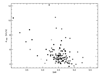
The radial velocity distribution of our sample, plotted in Figure 22, peaks at -1.7 $\pm$ 1.2 km s^-1 with a dispersion of 31.5 km s^-1. The dispersion in our distribution is slightly narrower than that obtained by Schmidt et al. (2010, overplotted as a dashed line for comparison), who derived a dispersion of 34.3 km s^-1 from a sample of 484 L dwarfs from SDSS. This discrepancy could be due to a geometric effect. Our sample is drawn from a smaller area of sky covering predominantly the northern galactic cap. The radial velocity of our sample is therefore dominated by the $W$ component of the galactic velocity, which is known to have a narrower dispersion than the $U$ and $V$ components (see e.g. Dehnen & Binney, 1998). We tested this hypothesis using the Besançon Model of stellar population synthesis of the Galaxy (Robin et al., 2003). For O to M type dwarfs with J $<$ 18.1 we obtain a dispersion of 34.8 km s^-1 when considering a sample spread over the SDSS footprint (i.e. the area covered by the Schmidt et al. 2010 sample) and a dispersion of 31.8 km s^-1 when considering a sample spread over the right ascension and declination limits of our sample (see Section 6.1). Both numbers are in good agreement with the observed ones, and the measured difference between our sample and Schmidt’s one seems therefore to be due to a geometric effect.

Another possible explanation is the fact that our sample is focused on field (i.e. thin disk) objects, and is therefore biased towards slightly younger dwarfs, i.e. towards a narrower $V_{\rm rad}$ distribution. Finally, the discrepancy could be due to errors in the determination of our radial velocities, introduced by uncorrected instability of X-shooter (which is however believed to be stable down to 0.5 km s^-1, Vernet et al., 2011).

The results presented in this section represent a feasibility study for a larger project to determine accurate and precise radial velocities for the brown dwarfs that will be observed by the European Space Agency mission Gaia. Further details on the project can be found in Marocco et al. (MmSAIt, in press).

6 Constraining the sub-stellar IMF and formation history

The Initial Mass Function (IMF) of stellar objects more massive than the Sun was first derived by Salpeter (1955), who parameterized it as $\Psi(m)\Delta m\propto(m/M_{\rm Sun})^{-\alpha}$ with $\alpha=2.35$ . The Salpeter IMF was later extended to less massive stars by Miller & Scalo (1979) who suggested that the IMF flattened below one solar mass. Currently the most widely accepted parameterizations are the log-normal IMF derived by Chabrier (2003, 2005) and the broken power law introduced by Kroupa (2001).

When trying to extend the IMF further into the sub-stellar regime, one is faced by one fundamental challenge. Sub-stellar objects do not form a main sequence, and keep on cooling down while evolving through the spectral sequence. As a result, there is no unique mass-luminosity relationship that one can use to convert the observed luminosity function (LF) into the IMF (this issue is sometimes referred to as age-mass-luminosity degeneracy). The observed luminosity function is therefore influenced by the formation history (or Birth Rate, hereafter BR) of this kind of objects, and one needs to take this into account while trying to constrain the IMF. While the BR is often assumed to be constant for stars (e.g. Miller & Scalo, 1979), it is unconstrained in the sub-stellar regime. Moreover, the formation mechanism of brown dwarfs and giant planets is not well understood. The different formation scenarios proposed would leave their imprints in the IMF and BR, so to distinguish between them it is fundamental to constrain these two quantities in the sub-stellar regime.

One way to break the age-mass-luminosity degeneracy is to look at young clusters and associations, since their known ages and metallicities allow the use of a mass-luminosity relation based on the cluster age, removing the dependency of the LF on the BR. Therefore they have been the target of many observational campaigns, e.g. Lodieu, Dobbie, & Hambly (2011); Lodieu et al. (2009, 2007); Caballero (2009); Luhman et al. (2009); Alves de Oliveira et al. (2013, 2012). These clusters allow a relatively direct measurement of the sub-stellar IMF, but the initial conditions and accretion histories of individual objects introduce uncertainties regarding the ages, and hence masses, of such young objects (e.g. Baraffe, 2010). Moreover, very high and variable extinction increases contamination by reddened field stars. Evolutionary models are also very uncertain at young ages, and the effect of magnetic activity or episodic accretion on the determination of luminosity are not yet fully understood. Finally, some of these regions are still forming stars, introducing further uncertainties and possible biases (see e.g. Alves de Oliveira, 2013).

Studying the IMF of the field populations has significant advantages, since there is a larger number of benchmark systems, and therefore the evolutionary and atmospheric models are more mature. Reddening is not an issue, given that even the deepest surveys can only probe the solar neighbourhood. On the other hand, the LF of field brown dwarfs depends on their BR, because only few field sub-stellar objects have age constraints, either as binaries (e.g. Burningham et al., 2011, 2010, 2009; Zhang et al., 2010; Day-Jones et al., 2011; Scholz et al., 2003; Gomes et al., 2013; Delorme et al., 2013) or as members of moving groups (e.g. Gagné et al., 2014; Malo et al., 2014, 2013; Clarke et al., 2010; Gálvez-Ortiz et al., 2010),. The assessment of completeness, contamination, and other observational biases can introduce further uncertainties.

Since the first attempt by Reid et al. (1999), several groups have made measurements of the sub-stellar mass function in the field. Due to the limited samples available, these measurements were either covering only L dwarfs (e.g Cruz et al., 2007) or only T dwarfs (e.g. Metchev et al., 2008; Burningham et al., 2013; Kirkpatrick et al., 2012; Reylé et al., 2010). Considering the full spectral sequence is in fact a challenge, and those studies that attempted this (e.g. Reylé et al., 2010) have been battling with high associated uncertainties and had to compromise with large bin sizes in order to get statistically significant sampling of the spectral sequence.

With modern large-scale near- and mid-infrared surveys, such as DENIS (Epchtein et al., 1999), SDSS (York et al., 2000), 2MASS (Skrutskie et al., 2006), UKIDSS (Lawrence et al., 2007), VHS (McMahon et al., 2013), and WISE (Wright et al., 2010), which have identified large numbers of brown dwarfs it is now possible to provide the necessary sample of such objects. In particular, while surveys like 2MASS and SDSS were more sensitive to the detection of L dwarfs than T dwarfs, the ULAS probes to greater depth and can provide a more even and statistically robust sampling of the full early-L to late-T range,. The L/T transition region, which is well populated by the sample presented here, is most sensitive to the BR.

This section outlines the efforts to use the sample of mid-L $-$ mid-T dwarfs presented here to empirically constrain the Galactic brown dwarf formation history. This sample is an obvious choice because it covers a large spectral type range (crucially focused on the L/T transition) with a good sampling of each spectral type bin, and it is complete (see Section 6.2), unbiased (see Section 2) and uncontaminated, since its members have been followed up with spectroscopy.

6.1 Determining the space density of L/T transition dwarfs

The spectroscopic follow-up of the full sample is incomplete. However, there are areas of sky where the follow-up is complete. So in order to determine the space density of brown dwarfs we divided the full sample in three sub-samples: between RA = 15h50m to 9h20m the follow-up is complete down to the limit of J = 18.1; between RA = 9h20m to 12h20m the follow-up is complete down to J = 17.87; finally between RA = 12h20m to 15h50m the follow-up is complete down to J = 17.7. These RA ranges correspond to an area of $\sim$ 620, 375 and 712 deg² in ULAS DR7, and account for 88, 29, and 50 objects respectively.

To determine the volume sampled we calculated the maximum distance at which an object of a given spectral type could have been detected (assuming the given magnitude limit), using the $M_{\rm J}$ -NIR spectral type relation from Marocco et al. (2010). With this distance limit we then calculated the volume sampled by each spectral type bin, and the corresponding space density of objects.

The derived space densities were then corrected for the Malmquist and Eddington biases following the approach described in Pinfield et al. (2008). The Eddington bias is caused by the photometric uncertainties on the magnitudes of objects near our cut (i.e. J $<$ 18.1). However, since the magnitude cut imposed is bright (it corresponds to a $\sim$ 12 $\sigma$ detection in the ULAS), the uncertainties at the J = 18.1 limit are typically less than $\sigma$ = 0.05 and therefore the Eddington bias correction is less than 1 per cent. This is negligible compared to the other sources of uncertainty. We estimated the Malmquist bias correction considering the mean scatter of the sample of known L and T dwarfs around the adopted $M_{\rm J}$ -NIR spectral type relation. This represents an increase in the volume sampled of 22 per cent.

To increase the number of objects per bin, and therefore reduce the Poisson errors, we binned up the sample in four spectral type bins: L0-L3, L4-L6, L7-T0, and T1-T4. These bins correspond roughly to effective temperature ranges of $\sim$ 150 K.

6.2 Completeness correction

In order to check the completeness of the sample, first we need to estimate the number of objects lost due to missed detections. As stated above, the imposed magnitude limit (J $<$ 18.1) is bright compared to the limit of the ULAS, and therefore we do not expect to lose any object because of missed detections. This is well demonstrated by Figure 23 where we show the number of objects detected in the original ULAS images as a function of MKO J magnitude. The number of faint sources increases as a power of ten (note that the y axis is in logarithmic scale) up to J $\sim$ 19 (as a consequence of the larger volume probed at fainter magnitudes, Mihalas & Binney, 1981), where it sharply drops. The dotted line is the fit to the bright tail of the distribution, i.e. for $14<$ J $<17$ . Extrapolating the fit up to J=18.1 and comparing the “expected” number of objects with the measured one gives a completeness of $>99\%$ . The number of objects lost due to incomplete detection in therefore negligible.

Another possible issue, especially when searching for faint objects, is the possible blending with bright sources. However the typical object density in the fields considered is very low, because we are probing regions outside the galactic plane, therefore blending should not be an issue. To quantitatively assess its impact we adopted the following approach. We used the ULAS J band images containing the selected objects. We run the Cambridge Astronomy Survey Unit (CASU) pipeline on the images to detect and extract all the sources in the field. We then doubled the number of objects in every image by taking a 20 $\times$ 20 pixels cut out around every object and copying it into a random position in the image, re-scaling it appropriately to blend the background level and avoid artefacts. We then re-run the CASU pipeline on the images and compared the number of sources identified (as a function of their J magnitude) with the number of sources in the original images. One would obviously expect to detect twice as many objects in the new synthetic images, with no dependence on the objects magnitude. This is indeed the case, as can be seen in Figure 23, where the number of detected objects in the synthetic images is plotted in red. With an average number of sources detected in the synthetic images of $\sim$ 1.987 time the number of sources detected in the original images (recovered sources after doubling / recovered sources prior to doubling = 15427/7764), and no clear dependence on the J magnitude, the incompleteness due to objects blending is 0.3 $\%$ , which is again negligible compared to the other causes of incompleteness considered below.

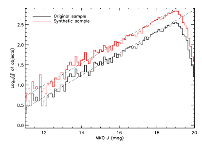
To assess the completeness of the photometric selection criteria, the sample was compared to a control sample of known L and T dwarfs taken from www.DwarfArchives.org, for a magnitude limit of J $\leq$ 16, removing any objects that are known to be members of unresolved binary systems. The control sample was cross-matched with the ULAS and SDSS in order to obtain photometry on the same colour system as the selection criteria used. The same set of colour cuts described in Section 2 was imposed to reveal the level of completeness of the sample selection. We retain all of the L4 dwarfs from the control sample, but only some of the L0-L3 dwarfs, indicating that the sample selection is complete for L4 spectral types and later. Similarly, the selection is largely incomplete beyond spectral types of T5. We therefore only consider the three spectral type bins covering the L4 $-$ T4 range.

The loss of objects due to photometric scattering of colours was also considered. For L4-L6 types one would expect to lose 3.7 dwarfs, this corresponds to a completeness level of 88 $\%$ . The L7-T0 range would lose 0.55 dwarfs, corresponding to a 94 $\%$ completeness; for T1-T4 the expected loss is 0.05 dwarfs, corresponding to a completeness of 99 $\%$ .

Pixel-noise correlation is not an issue, as demonstrated by Andrews et al. (2014), who estimated the randomness of background noise in the ULAS images by visually selecting 11 empty 7 $\times$ 7 pixel regions from the mosaics. They computed the standard deviation of the mean pixel value of each region (calling it $q$ ) and compared it against a similar calculation after randomly swapping pixels between regions. A $q/q_{\rm swapped}$ of 1 indicates perfectly uncorrelated noise while $q/q_{\rm swapped}\gg 1$ is due to non-pixel scale systematic variations. For ULAS images they found $q/q_{\rm swapped}\sim 1$ .

6.3 Correction for unresolved binarity

We also corrected the results for the presence of binaries by first considering objects identified as possible binaries (Section 3.2) for which the spectral deconvolution gives a statistically “better fit”. We derived the J magnitude of the two components given the unresolved photometry and the two spectral types determined with the deconvolution, and removed from the sample all companions and those primaries that would fall beyond the magnitude limit.

To assess the completeness of this correction we performed numerical simulations, using the spectral templates taken from the SpeX-Prism library. The spectra were combined to create a sample of synthetic unresolved binaries, following the procedure described in ADJ13 and in Section 3.2 of this work. The synthetic templates were “degraded” to the typical SNR of the observed spectra by adding gaussian noise. We then run the binary identification process on each of the synthetic binaries to calculate the rate of successful detections. To avoid false positive detections in low mass ratio binaries, when fitting a given synthetic binary we removed from the template list all the synthetic binaries that had the same primary as the “target” one. For example, when fitting the synthetic binary SDSS J165329.69+623136.5 + 2MASSI J0415195 $-$ 093506 (L1.0 + T8.0) we removed from the set of templates all the synthetic binaries that had SDSS J165329.69+623136.5 as a primary. This is because one can expect that the synthetic L1.0 + T8.0 SDSS J165329.69+623136.5 + HD 3651B would fit better the target than an L1.0 template alone, not because the synthetic binary genuinely fits better, but because the contribution from the T8.0 component is negligible and we would essentially be fitting the L1.0 component with itself.

The results are shown in Figure 24, where we plot the fraction of synthetic binaries retrieved as a function of the spectral type of the two components. Interpolated contour level are overplotted to ease the reading of the Figure. As expected, the technique is most efficient at the L/T transition, and the fraction of detected binaries steeply declines when moving towards very low mass ratios and early L type binaries. Equal spectral type binaries are also not detectable with this method. Overplotted as black circles are the binary candidates identified in Section 3.2. Not surprisingly the candidates are concentrated mostly in the high detection fraction area.

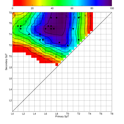
The sample of binary candidates is probably contaminated by peculiar objects, and therefore the derived binary fraction is somewhat higher than the “true” one. To assess the level of contamination we run the binary identification method on a sample of L and T dwarfs that have been previously targeted by high-resolution imaging campaigns, and have not showed evidences of binarity. The control sample consists of 40 objects covering the L0.0 to T7.5 spectral range, and includes objects taken from Bouy et al. (2003), Gizis et al. (2003), and Burgasser et al. (2006). Two out of 40 objects are flagged as binaries by the detection method, implying a level of contamination of $5\%$ .

We can now use the detected binaries to constrain the binary fraction. To do that we combine the detection probability from Figure 24 with the mass-ratio distribution of sub-stellar binaries from Figure 3 of Burgasser et al. (2007). First of all we correct the observed number of binaries for contamination using the fraction derived above, and then for completeness using the detection probability. All these binaries have mass ratio $q<$ 1, if not they would have equal spectral type. Using the distribution from Burgasser et al. (2007) we could estimate the number of undetected equal mass/equal spectral type binaries and therefore derive the binary fraction. However the exact mass ratio of a system depends on its age, which is unconstrained. So we can only correct the number of observed binaries using the ratio between the number of $q$ =1 binaries over the number of $q<$ 1 binaries, which is $\sim$ 1.2.

The numbers derived are presented in Table 7. We calculated the binary fraction in the three spectral type ranges considered above (i.e. L4-L6, L7-T0, and T1-T4). The fraction is 24 $\%$ in the L4-L6 range but rises to $\sim$ 70 $\%$ in the L7-T0 range, before dropping down to $\sim$ 40 $\%$ in the early T regime. This variations could be partly due to an underestimate of the number of equal spectral type binaries in the early L regime, due to the fact that the detected binary candidates lie in the $q\ll$ 1 range, and the ratio of $(q=1)/(q\ll 1)$ binaries is higher than the assumed value of $\sim$ 1.2.

High-resolution imaging and radial velocity surveys typically detect a binary fraction of $\sim$ 10-20 $\%$ for brown dwarfs (e.g. Joergens, 2008; Kurosawa, Harries, & Littlefair, 2006; Basri & Reiners, 2006). Many studies however report an higher observed binary fraction in the L/T transition regime (e.g. Liu et al., 2006; Burgasser, 2007; Burgasser et al., 2006), with values around $\approx 40\%$ . The binary fraction obtained here is even higher, peaking at $\sim$ 70 $\%$ in the L7-T0 range. The reason for this discrepancy could be in an higher false positive ratio than estimated here. The control sample used to determine the contamination is in fact limited (only 40 objects) and the L/T transition in particular is poorly sampled. When correcting the derived space densities for unresolved binarity we will therefore use both the binary fraction we measured, and the values published in the literature.

Spectral	Total number	$q<$ 1		$q=$ 1
type range	of objects	Binary fraction	Binaries	Binary fraction	Binaries
L4 $-$ L6	54	11 $\%$	5.8	13 $\%$	7.0
L7 $-$ T0	19	34 $\%$	7.1	40 $\%$	8.5
T1 $-$ T4	16	19 $\%$	4.7	23 $\%$	5.6

Table 7: The derived binary fraction. For each spectral type range we indicate the binary fraction and the expected number of binaries in the sample.

To take into account the presence of the undetected equal spectral type binaries, which would fall beyond the J limit if they were single objects, we used the definition of “observed binary fraction” given by Burgasser et al. (2003),

\frac{N_{B}}{N_{m}}=\frac{\gamma}{\gamma+(1/{\rm BF})-1}

(2)

where $N_{B}$ and $N_{m}$ are the observed binaries and the total number of systems, respectively, BF is the “true” binary fraction, and $\gamma$ is the fractional increase in volume due to inclusion of binaries in the sample. The number of binaries that fall within the magnitude limit because of their increased brightness ( $N_{D}$ ) is

\frac{N_{D}}{N_{B}}=\frac{\gamma-1}{\gamma}

(3)

Therefore, the fraction of objects to be excluded from the sample ( $f_{\rm excl}$ ) is

f_{\rm excl}=\frac{N_{B}}{N_{m}}\frac{N_{D}}{N_{B}}=\frac{\gamma-1}{\gamma+(1/{\rm BF})-1}

(4)

For equal spectral type binaries $\gamma=2\sqrt{2}$ .

As stated above, the final correction applied was derived assuming BF $=26\pm 13\%$ , i.e. the mid point between the upper and lower limit to the $q=1$ binary fraction derived in this work, and BF $=14\pm 10\%$ , i.e. the weighted average of the values presented in the literature. The corrections applied are therefore $f_{\rm excl}=0.30\pm 0.10$ and $f_{\rm excl}=0.18\pm 0.12$ .

6.4 Comparison with numerical simulations

We compared the space densities obtained above with the results of numerical simulations computed assuming different IMFs and birth rates from Deacon & Hambly (2006). Details of the simulations are briefly summarized here.

They assume a power-law IMF in the form

\Psi(M)\propto M^{-\alpha}\left(pc^{-3}M^{-1}_{\odot}\right)

(5)

where $\Psi(M)$ is the number of objects per unit volume in a given mass interval. They also assumed an exponential birth rate of the form

b(t)\propto e^{-\beta t}

(6)

where $t$ is in Gyr and $\beta$ is the inverse of the birth rate scale time $\tau$ (in Gyr, since the galaxy was formed). Each simulated object was assigned an age based on the birth rate and a mass based on the IMF, giving a final creation function $C$ given by the equation

C(M,t)=\Psi(M)\frac{b(t)}{T_{G}}

(7)

where $T_{G}$ is the age of the Galaxy. $C$ is therefore the number of objects created per unit time per unit mass. The evolution of each object and its parameters (i.e. $T_{\rm eff}$ and absolute magnitudes) were calculated using the evolutionary models from Baraffe et al. (1998). Any model-dependent systematics would be introduced, but these should not affect the overall trend. The $T_{\rm eff}$ of an object was then converted into a spectral type using the $T_{\rm eff}$ -NIR spectral type relation presented in Stephens et al. (2009, equation 3). The number densities obtained for each bin were finally normalized to 0.0024 pc^-3 in the 0.1-0.09 $M_{\odot}$ mass range, according to Deacon, Nelemans, & Hambly (2008). We consider the simulations for three different values of $\beta$ (0.0, 0.2, and 0.5 corresponding to $\tau$ = $\infty$ , 5, and 2 Gyr, respectively) and three values of $\alpha$ (+1.0, 0.0, -1.0). The results obtained are shown in Figure 25, where different colours represent different values of $\alpha$ and different line styles represent different values of $\beta$ .

We compared the calculated space densities, taking into account the completeness and contribution from unresolved binaries, with those presented by various authors in the literature. We considered five different studies: Cruz et al. (2007), Metchev et al. (2008), Reylé et al. (2010), Kirkpatrick et al. (2012), Burningham et al. (2013), and Day-Jones et al. (2013).

The Cruz et al. (2007) space densities probe down to the 2MASS limit (J = $\sim$ 16) and cover the M9-L8 dwarfs, likely suffering from incompleteness at the later types due to colour scattering. The binary correction uses the observed binary fraction of $\sim 17\%$ derived via high-resolution imaging of their sample. Metchev et al. (2008) cross-matched 2MASS with SDSS DR1 and used a series of colour selection criteria to select a sample of L and T dwarfs down to $z\leq$ 21. The correction for binarity assumes only the existence of equal mass/equal spectral type binaries for reason of the strong peak in the $q$ distribution (Burgasser et al., 2007, Figure 3). The adopted binary fraction is assumed to decline from $50\%$ in the T0-T2.5 range, down to $21\%$ in the T3-T5.5 range, to $13\%$ in the T6-T8 range, and is therefore comparable to the numbers derived here. Reylé et al. (2010) used CFBDS to select and classify a sample of $\sim$ 100 $>$ L5 dwarfs down to $z^{\prime}<$ 22.5, a comparable depth to this sample. They chose not make any correction for binarity, given the large uncertainty in the measured binary fraction. Kirkpatrick et al. (2012) focused on the late T and Y dwarfs, using the WISE-selected sample of nearby objects. Assuming a binary fraction of $30\%$ and correcting for the incompleteness at the faint end of their sample, they derive the space density in the T6 to Y0.5 range. The Burningham et al. (2013) space densities use the same $M_{\rm J}$ -spectral type relations we adopted. They correct for binarity assuming an upper limit on the binary fraction of 45 $\%$ (Maxted & Jeffries, 2005) and a lower limit of 5 $\%$ Burgasser et al. (2003), hence deriving two values of the space density in each spectral type bin. They also probe down to a magnitude limit comparable to this sample. Finally, Day-Jones et al. (2013) represent an early result from this sample, obtained from the sub-sample falling in the RA = 22h to 4h range. The only difference in the treatment of the data is in the binary correction, since in Day-Jones et al. (2013) we followed the approach of Burningham et al. (2013) and derived two values for each spectral type range.

Our results and those listed above are summarized in Table 8, and in Figure 25. It is important to notice that the numbers in Table 8 are integrated over the spectral range quoted, while those plotted in Figure 25 are per spectral type, to allow a direct comparison with the simulations. A first look at the plot shows that our space densities do not differ drastically (within uncertainties) from those previously measured and discussed earlier. The differences between our derived densities and those previously published are mostly due to the use of different $M_{\rm J}$ -SpT conversions and different binary fractions by the various groups.

Reference	Spectral type range	Space density ( $\times 10^{-3}$ pc^-3)
Cruz et al. (2007)	L0-L3	1.7 $\pm$ 0.4
Cruz et al. (2007)	L3.5-L8	2.2 $\pm$ 0.4
Metchev et al. (2008)	T0-T2.5	0.86 ${}^{+0.48}_{-0.44}$
	T3-T5.5	1.4 ${}^{+0.8}_{-0.8}$
	T6-T8	4.7 ${}^{+3.1}_{-2.8}$
Reylé et al. (2010)	L5-T0	2.0 ${}^{+0.8}_{-0.7}$
	T0.5-T5.5	1.4 ${}^{+0.3}_{-0.2}$
	T6-T8	5.3 ${}^{+3.1}_{-2.2}$
Kirkpatrick et al. (2012)	T6-T6.5	1.1
	T7-T7.5	0.93
	T8-T8.5	1.4
	T9-T9.5	1.6
Burningham et al. (2013)	T6-T6.5	0.39 $\pm$ 0.22 $-$ 0.71 $\pm$ 0.40
	T7-T7.5	0.56 $\pm$ 0.32 $-$ 1.02 $\pm$ 0.64
	T8-T8.5	2.05 $\pm$ 1.21 $-$ 3.79 $\pm$ 2.24
Day-Jones et al. (2013)	L4-L6.5	0.53 $\pm$ 0.10 $-$ 0.88 $\pm$ 0.16
	L7-T0.5	0.56 $\pm$ 0.10 $-$ 0.94 $\pm$ 0.16
	T1-T4.5	0.42 $\pm$ 0.16 $-$ 0.71 $\pm$ 0.27
This paper, BF = 26 $\pm$ 13	L4-L6.5	0.85 $\pm$ 0.55
	L7-T0.5	0.73 $\pm$ 0.47
	T1-T4.5	0.74 $\pm$ 0.48
This paper, BF = 14 $\pm$ 10	L4-L6.5	1.00 $\pm$ 0.64
	L7-T0.5	0.85 $\pm$ 0.55
	T1-T4.5	0.88 $\pm$ 0.56

Table 8: The space density derived here compared to values presented in the literature. The numbers are integrated over the spectral range quoted in the second column.

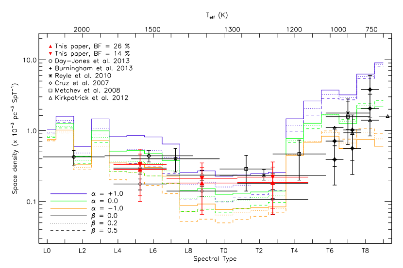
The most apparent feature is the absence of a significant drop in the number of objects between L7 and T4. The number of L/T transition dwarfs decreases, but not as much as expected. For the predicted theoretical deficit to be realised a higher binary fraction than assumed for the L/T transition would be necessary. That would lead to a larger correction and therefore to lower space densities. Conversely, a lower binary fraction at early types would bring up the density of objects in the L4-L6 range increasing the drop.

However, this second scenario would lead to a preference for $\alpha>0$ , which would be inconsistent with the results for late type objects, that consistently point towards $\alpha<0$ . On the other hand, $\alpha>0$ is found also in nearby young clusters (e.g. Casewell et al., 2007; Bastian, Covey, & Meyer, 2010) and by microlensing surveys ( $\alpha=0.49^{+0.24}_{-0.27}$ , Sumi et al., 2011).

To reconcile the results in the two temperature regimes, one could assume that the binary fraction in the L/T transition is much higher than currently estimated. An alternative explanation is that objects in the high-mass end and low-mass end form in different environments, with the high-mass brown dwarfs forming predominantly in dense clusters (i.e. resulting in an $\alpha>0$ IMF) and the low-mass brown dwarfs forming in low density environments, leading to a $\alpha<0$ IMF (Kroupa et al., 2013). Another possibility, as suggested by Burningham et al. (2013), is that the cooling times assumed to transform the IMF into field luminosity function are affected by systematic errors.

As regards the formation history, it is not currently possible to place robust constraints on the birth rate with this sub-sample. One of the largest sources of uncertainties is the binary fraction. This could be resolved with the follow-up of the unresolved binary candidates identified here, by either AO imaging or radial velocity.

The other main source of uncertainty is the absolute magnitude $-$ spectral type calibration. Although based on an increasing number of objects with well measured parallaxes, the scatter around the current polynomial relation is still large, with typical rms of 0.4 magnitudes (Dupuy & Liu, 2012), and this propagates into a factor of $\sim$ 1.5 in the volume sampled.

7 Conclusions

In this contribution we have presented the spectroscopic analysis of a sample of 196 late-M, L, and T dwarfs from the UKIDSS LAS DR7. One hundred and twenty two of these represent new discoveries. Among this large sample of objects we have identified 22 peculiar blue L dwarfs and 2 blue T dwarfs, that further increase the population of this class of objects. Suspected to pertain to a slightly older disk population (therefore slightly metal depleted) the kinematics are fundamental to fully characterize these new objects.

We have also identified 2 peculiar low-gravity late-M dwarfs, potentially young objects that can constitute useful benchmarks to study low-gravity atmospheres and constrain early evolution models. Once again the kinematics will be fundamental to confirm or refute their youth.

Using an index-based selection technique coupled with spectral deconvolution, we also identified 27 unresolved binary candidates among our targets. These objects are particularly important as their follow-up constraint on the population properties of multiple sub-stellar systems, and offer hints into the understanding of their formation mechanism.

The sample presented here, being complete, unbiased, and uncontaminated, represents an opportunity to measure the luminosity function of field sub-stellar objects. Our attempt to use the measured space density has however been limited by two fundamental uncertainties. One is the lack of knowledge of the binary fraction. Following up the binary candidates identified here can represent a first step forward towards a more precise constraint of this important observable parameter. In the near future the ESA mission Gaia will provide a more accurate measurement, significantly reducing this source of uncertainty. The other is the use of photometric distances to compute the volume sampled, and the large associated uncertainty due to the scatter of objects around the “main sequence”. Only measuring trigonometric parallaxes for a large sample of brown dwarfs would remove this uncertainty, and the astrometric programs focusing on sub-stellar objects represent an encouraging step forward in this direction.

Although limited by these uncertainties, the space densities derived here nevertheless point toward an higher than expected ratio of L/T transition dwarfs to late-Ts. If we assume a power-law IMF with a negative exponent (as suggested by the LF of late-T dwarfs), then the observed density of L/T transition objects is almost a factor of two higher than expected. This discrepancy can be suggestive of a higher than expected binary fraction in the L/T transition range, or that the cooling times assumed to transform the IMF into field LF are affected by systematic errors, or that low-mass and high-mass brown dwarfs are predominantly the product of different formation mechanisms and therefore derive from different underlying IMFs.

The full exploitation of present surveys is revealing larger and larger populations of L, T, and Y dwarfs, and new facilities like SPHERE and GPI will push the boundaries of our observations towards lower and lower masses. Moreover the already mentioned ESA/Gaia mission will provide a more accurate calibration of the absolute magnitude sequence and a more robust constraint on the binary fraction. Therefore it seems we are now approaching a more reliable determination of the sub-stellar IMF and BR, that will lead to a better understanding of their formation.

Acknowledgments

We thank the referee, John Gizis, for comments that have significantly improved the quality of this paper.

FM would like to thank Antonio Chrysostomou and Philippe Delorme for the useful discussions and their valuable suggestions.

This research is based on observations collected at the European Organisation for Astronomical Research in the Southern Hemisphere, Chile programs 086.C-0450, 087.C-0639, 088.C-0048, and 091.C-0452.

The authors would like to acknowledge the Marie Curie 7th European Community Framework Programme grant n.247593 Interpretation and Parameterization of Extremely Red COOL dwarfs (IPERCOOL) International Research Staff Exchange Scheme. FM would like to acknowledge the support received from the European Science Foundation (ESF) within the framework of the ESF activity entitled “Gaia Research for European Astronomy Training”, Exchange Grant number 4641.

This research has made use of: the SIMBAD database operated at CDS France; the SpeX Prism Spectral Libraries, maintained by Adam Burgasser at http://pono.ucsd.edu/ $\sim$ adam/browndwarfs/spexprism; and, the M, L, and T dwarf compendium housed at dwarfArchives.org and maintained by Chris Gelino, Davy Kirkpatrick, and Adam Burgasser.

References

Allard, Homeier, & Freytag (2011) Allard F., Homeier D., Freytag B., 2011, ASPC, 448, 91
Allers & Liu (2013) Allers K. N., Liu M. C., 2013, ApJ, 772, 79
Alves de Oliveira et al. (2012) Alves de Oliveira C., Moraux E., Bouvier J., Bouy H., 2012, A&A, 539, A151
Alves de Oliveira et al. (2013) Alves de Oliveira C., et al., 2013, A&A, 559, A126
Alves de Oliveira (2013) Alves de Oliveira C., 2013, MmSAI, 84, 905
Andrei et al. (2011) Andrei A. H., et al., 2011, AJ, 141, 54
Andrews et al. (2014) Andrews S. K., Kelvin L. S., Driver S. P., Robotham A. S. G., 2014, PASA, 31, 4
Baraffe et al. (1998) Baraffe I., Chabrier G., Allard F., Hauschildt P. H., 1998, A&A, 337, 403
Baraffe (2010) Baraffe I., 2010, HiA, 15, 755
Basri & Reiners (2006) Basri G., Reiners A., 2006, AJ, 132, 663
Bastian, Covey, & Meyer (2010) Bastian N., Covey K. R., Meyer M. R., 2010, ARA&A, 48, 339
Blake, Charbonneau, & White (2010) Blake C. H., Charbonneau D., White R. J., 2010, ApJ, 723, 684
Bouy et al. (2003) Bouy H., Brandner W., Martín E. L., Delfosse X., Allard F., Basri G., 2003, AJ, 126, 1526
Borysow, Jorgensen, & Zheng (1997) Borysow A., Jorgensen U. G., Zheng C., 1997, A&A, 324, 185
Burgasser et al. (2000) Burgasser A. J., et al., 2000, ApJ, 531, L57
Burgasser et al. (2003) Burgasser A. J., Kirkpatrick J. D., Reid I. N., Brown M. E., Miskey C. L., Gizis J. E., 2003, ApJ, 586, 512
Burgasser et al. (2006) Burgasser A. J., Geballe T. R., Leggett S. K., Kirkpatrick J. D., Golimowski D. A., 2006, ApJ, 637, 1067
Burgasser et al. (2006) Burgasser A. J., Kirkpatrick J. D., Cruz K. L., Reid I. N., Leggett S. K., Liebert J., Burrows A., Brown M. E., 2006, ApJS, 166, 585
Burgasser (2007) Burgasser A. J., 2007, ApJ, 659, 655
Burgasser et al. (2007) Burgasser A. J., Reid I. N., Siegler N., Close L., Allen P., Lowrance P., Gizis J., 2007, Protostars and Planets V, 427
Burgasser et al. (2010) Burgasser A. J., Cruz K. L., Cushing M., Gelino C. R., Looper D. L., Faherty J. K., Kirkpatrick J. D., Reid I. N., 2010, ApJ, 710, 1142
Burningham et al. (2009) Burningham B., et al., 2009, MNRAS, 395, 1237
Burningham et al. (2010) Burningham B., et al., 2010, MNRAS, 404, 1952
Burningham et al. (2010) Burningham B., et al., 2010, MNRAS, 406, 1885
Burningham et al. (2011) Burningham B., et al., 2011, MNRAS, 414, 3590
Burningham et al. (2013) Burningham B., et al., 2013, MNRAS, 433, 457
Burrows et al. (1997) Burrows A., et al., 1997, ApJ, 491, 856
Burrows, Sudarsky, & Hubeny (2006) Burrows A., Sudarsky D., Hubeny I., 2006, ApJ, 640, 1063
Caballero (2009) Caballero J. A., 2009, AIPC, 1094, 912
Casewell et al. (2007) Casewell S. L., Dobbie P. D., Hodgkin S. T., Moraux E., Jameson R. F., Hambly N. C., Irwin J., Lodieu N., 2007, MNRAS, 378, 1131
Chabrier (2005) Chabrier G., 2005, ASSL, 327, 41
Chabrier (2003) Chabrier G., 2003, PASP, 115, 763
Chiu et al. (2006) Chiu K., Fan X., Leggett S. K., Golimowski D. A., Zheng W., Geballe T. R., Schneider D. P., Brinkmann J., 2006, AJ, 131, 2722
Clarke et al. (2010) Clarke J. R. A., et al., 2010, MNRAS, 402, 575
Cruz et al. (2007) Cruz K. L., et al., 2007, AJ, 133, 439
Cruz, Kirkpatrick, & Burgasser (2009) Cruz K. L., Kirkpatrick J. D., Burgasser A. J., 2009, AJ, 137, 3345
Day-Jones et al. (2008) Day-Jones A. C., et al., 2008, MNRAS, 388, 838
Day-Jones et al. (2011) Day-Jones A. C., et al., 2011, MNRAS, 410, 705
Day-Jones et al. (2013) Day-Jones A. C., et al., 2013, MNRAS, 430, 1171
Deacon & Hambly (2006) Deacon N. R., Hambly N. C., 2006, MNRAS, 371, 1722
Deacon, Nelemans, & Hambly (2008) Deacon N. R., Nelemans G., Hambly N. C., 2008, A&A, 486, 283
Dehnen & Binney (1998) Dehnen W., Binney J. J., 1998, MNRAS, 298, 387
Delorme et al. (2013) Delorme P., et al., 2013, A&A, 553, L5
Dupuy & Liu (2012) Dupuy T. J., Liu M. C., 2012, ApJS, 201, 19
Epchtein et al. (1999) Epchtein N., et al., 1999, A&A, 349, 236
Faherty et al. (2009) Faherty J. K., Burgasser A. J., Cruz K. L., Shara M. M., Walter F. M., Gelino C. R., 2009, AJ, 137, 1
Faherty et al. (2010) Faherty J. K., Burgasser A. J., West A. A., Bochanski J. J., Cruz K. L., Shara M. M., Walter F. M., 2010, AJ, 139, 176
Faherty et al. (2012) Faherty J. K., et al., 2012, ApJ, 752, 56
Fan et al. (2000) Fan X., et al., 2000, AJ, 119, 928
Gagné et al. (2014) Gagné J., Lafrenière D., Doyon R., Malo L., Artigau É., 2014, ApJ, 783, 121
Gálvez-Ortiz et al. (2010) Gálvez-Ortiz M. C., et al., 2010, MNRAS, 409, 552
Geballe et al. (2002) Geballe T. R., et al., 2002, ApJ, 564, 466
Gelino, Kulkarni, & Stephens (2006) Gelino C. R., Kulkarni S. R., Stephens D. C., 2006, PASP, 118, 611
Gizis et al. (2003) Gizis J. E., Reid I. N., Knapp G. R., Liebert J., Kirkpatrick J. D., Koerner D. W., Burgasser A. J., 2003, AJ, 125, 3302
Gomes et al. (2013) Gomes J. I., et al., 2013, MNRAS, 431, 2745
Gorlova et al. (2003) Gorlova N. I., Meyer M. R., Rieke G. H., Liebert J., 2003, ApJ, 593, 1074
Hawley et al. (2002) Hawley S. L., et al., 2002, AJ, 123, 3409
Hewett et al. (2006) Hewett P. C., Warren S. J., Leggett S. K., Hodgkin S. T., 2006, MNRAS, 367, 454
Joergens (2008) Joergens V., 2008, A&A, 492, 545
Jones et al. (1996) Jones H. R. A., Longmore A. J., Allard F., Hauschildt P. H., 1996, MNRAS, 280, 77
Kirkpatrick et al. (2000) Kirkpatrick J. D., et al., 2000, AJ, 120, 447
Kirkpatrick (2005) Kirkpatrick J. D., 2005, ARA&A, 43, 195
Kirkpatrick et al. (2010) Kirkpatrick J. D., et al., 2010, ApJS, 190, 100
Kirkpatrick et al. (2012) Kirkpatrick J. D., et al., 2012, ApJ, 753, 156
Knapp et al. (2004) Knapp G. R., et al., 2004, AJ, 127, 3553
Kroupa (2001) Kroupa P., 2001, MNRAS, 322, 231
Kroupa et al. (2013) Kroupa P., Weidner C., Pflamm-Altenburg J., Thies I., Dabringhausen J., Marks M., Maschberger T., 2013, Planets, Stars and Stellar Systems. Volume 5: Galactic Structure and Stellar Populations, 115
Kurosawa, Harries, & Littlefair (2006) Kurosawa R., Harries T. J., Littlefair S. P., 2006, MNRAS, 372, 1879
Lawrence et al. (2007) Lawrence A., et al., 2007, MNRAS, 379, 1599
Leggett et al. (2000) Leggett S. K., et al., 2000, ApJ, 536, L35
Leggett et al. (2009) Leggett S. K., et al., 2009, ApJ, 695, 1517
Liu et al. (2006) Liu M. C., Leggett S. K., Golimowski D. A., Chiu K., Fan X., Geballe T. R., Schneider D. P., Brinkmann J., 2006, ApJ, 647, 1393
Liu, Leggett, & Chiu (2007) Liu M. C., Leggett S. K., Chiu K., 2007, ApJ, 660, 1507
Luhman et al. (2009) Luhman K. L., Mamajek E. E., Allen P. R., Cruz K. L., 2009, ApJ, 703, 399
Lodieu et al. (2007) Lodieu N., Dobbie P. D., Deacon N. R., Hodgkin S. T., Hambly N. C., Jameson R. F., 2007, MNRAS, 380, 712
Lodieu et al. (2009) Lodieu N., Zapatero Osorio M. R., Rebolo R., Martín E. L., Hambly N. C., 2009, A&A, 505, 1115
Lodieu, Dobbie, & Hambly (2011) Lodieu N., Dobbie P. D., Hambly N. C., 2011, A&A, 527, A24
Looper et al. (2008) Looper D. L., et al., 2008, ApJ, 686, 528
Lucas et al. (2001) Lucas P. W., Roche P. F., Allard F., Hauschildt P. H., 2001, MNRAS, 326, 695
Malo et al. (2013) Malo L., Doyon R., Lafrenière D., Artigau É., Gagné J., Baron F., Riedel A., 2013, ApJ, 762, 88
Malo et al. (2014) Malo L., Artigau É., Doyon R., Lafrenière D., Albert L., Gagné J., 2014, arXiv, arXiv:1402.6053
Marley et al. (2002) Marley M. S., Seager S., Saumon D., Lodders K., Ackerman A. S., Freedman R. S., Fan X., 2002, ApJ, 568, 335
Marocco et al. (2010) Marocco F., et al., 2010, A&A, 524, A38
Marocco et al. (2013) Marocco F., et al., 2013, AJ, 146, 161
Marocco et al. (2014) Marocco F., et al., 2014, MNRAS, 439, 372
Martín et al. (1999) Martín E. L., Delfosse X., Basri G., Goldman B., Forveille T., Zapatero Osorio M. R., 1999, AJ, 118, 2466
Maxted & Jeffries (2005) Maxted P. F. L., Jef0fries R. D., 2005, MNRAS, 362, L45
McMahon et al. (2013) McMahon R. G., Banerji M., Gonzalez E., Koposov S. E., Bejar V. J., Lodieu N., Rebolo R., VHS Collaboration, 2013, Msngr, 154, 35
Metchev et al. (2008) Metchev S. A., Kirkpatrick J. D., Berriman G. B., Looper D., 2008, ApJ, 676, 1281
Mihalas & Binney (1981) Mihalas D., Binney J., 1981, San Francisco, CA, W. H. Freeman and Co., 1981. 608 p.
Miller & Scalo (1979) Miller G. E., Scalo J. M., 1979, ApJS, 41, 513
Murray et al. (2011) Murray D. N., et al., 2011, MNRAS, 414, 575
Pinfield et al. (2008) Pinfield D. J., et al., 2008, MNRAS, 390, 304
Pinfield et al. (2012) Pinfield D. J., et al., 2012, MNRAS, 422, 1922
Press, Flannery, & Teukolsky (1986) Press W. H., Flannery B. P., Teukolsky S. A., 1986, Cambridge: University Press, 1986
Reid et al. (1999) Reid I. N., et al., 1999, ApJ, 521, 613
Reid, Gizis, & Hawley (2002) Reid I. N., Gizis J. E., Hawley S. L., 2002, AJ, 124, 2721
Reylé et al. (2010) Reylé C., et al., 2010, A&A, 522, A112
Robin et al. (2003) Robin A. C., Reylé C., Derrière S., Picaud S., 2003, A&A, 409, 523
Salpeter (1955) Salpeter E. E., 1955, ApJ, 121, 161
Schmidt et al. (2010) Schmidt S. J., West A. A., Hawley S. L., Pineda J. S., 2010, AJ, 139, 1808
Scholz et al. (2003) Scholz R.-D., McCaughrean M. J., Lodieu N., Kuhlbrodt B., 2003, A&A, 398, L29
Scholz (2010) Scholz R.-D., 2010, A&A, 510, L8
Skrutskie et al. (2006) Skrutskie M. F., et al., 2006, AJ, 131, 1163
Stephens et al. (2009) Stephens D. C., et al., 2009, ApJ, 702, 154
Stumpf et al. (2009) Stumpf M. B., Brandner W., Köhler R., Bouy H., Henning T., 2009, AIPC, 1094, 561
Sumi et al. (2011) Sumi T., et al., 2011, Natur, 473, 349
Taylor (1992) Taylor J. H., 1992, RSPTA, 341, 117
Tsuji & Nakajima (2003) Tsuji T., Nakajima T., 2003, ApJ, 585, L151
Vernet et al. (2011) Vernet J., et al., 2011, A&A, 536, A105
Wright et al. (2010) Wright E. L., et al., 2010, AJ, 140, 1868
York et al. (2000) York D. G., et al., 2000, AJ, 120, 1579
Zhang et al. (2010) Zhang Z. H., et al., 2010, MNRAS, 404, 1817
Zhang et al. (2013) Zhang Z. H., et al., 2013, MNRAS, 434, 1005

Appendix A Observations log

We present in Table LABEL:obs_log the log of the observations for our targets. For each object we show the date of observation, the standard used for telluric correction with its spectral type indicated in brackets, and the spectrophotometric standard used for flux calibration. Objects are referred to using their short ID, for the full ID and coordinates, please see Table LABEL:types.

ID	Observation date	Telluric	Spectrophotometric
	(YYYY-MM-DD)	standard (type)	standard
BRLT1	2011-09-19	HIP 014898 (B3V)	LTT 7987
BRLT2	2011-09-20	HIP 105164 (B5V)	LTT 7987
BRLT3	2010-11-28	HIP 038896 (B3V)	GD 71
BRLT5	2010-11-27	HIP 018926 (B3V)	GD 71
BRLT6	2011-09-18	HIP 013327 (B7V)	LTT 7987
BRLT7	2011-09-20	HIP 105164 (B5V)	LTT 7987
BRLT8	2011-09-21	HD 1160 (A0V)	LTT 7987
BRLT9	2011-09-19	HIP 014898 (B3V)	LTT 7987
BRLT10	2010-11-29	HIP 037502 (B2V)	GD 71
BRLT12	2011-09-21	HIP 014972 (B8V)	LTT 7987
BRLT14	2010-11-30	HIP 043520 (B3V)	GD 71
BRLT15	2011-09-20	HIP 001191 (B9V)	LTT 7987
BRLT16	2010-11-28	HIP 038896 (B3V)	GD 71
BRLT18	2010-11-30	HIP 041463 (B2V)	GD 71
BRLT20	2011-09-21	HIP 014972 (B8V)	LTT 7987
BRLT21	2010-11-27	HIP 018926 (B3V)	GD 71
BRLT22	2011-09-21	HD 216009 (A0V)	LTT 7987
BRLT24	2011-09-21	HD 216009 (A0V)	LTT 7987
BRLT26	2010-11-27	HIP 044423 (B6V)	GD 71
BRLT27	2010-11-29	HIP 017734 (B8V)	GD 71
BRLT28	2011-10-04	HIP 105164 (B5V)	LTT 7987
BRLT30	2010-11-28	HIP 041386 (B8V)	GD 71
BRLT31	2011-09-18	HIP 013327 (B7V)	LTT 7987
BRLT32	2011-09-20	HIP 001191 (B9V)	LTT 7987
BRLT33	2011-09-19	HD 8864 (B1V)	LTT 7987
BRLT35	2011-09-21	HD 2811 (A3V)	LTT 7987
BRLT37	2011-09-18	HIP 029429 (B1V)	LTT 7987
BRLT38	2010-11-27	HIP 044423 (B6V)	GD 71
BRLT39	2011-09-18	HIP 029429 (B1V)	LTT 7987
BRLT40	2010-11-29	HIP 017734 (B8V)	GD 71
BRLT42	2011-09-20	HIP 022840 (B5V)	LTT 7987
BRLT44	2010-11-30	HIP 026450 (B7V)	GD 71
BRLT45	2011-09-21	HD 2811 (A3V)	LTT 7987
BRLT46	2010-11-30	HIP 041463 (B2V)	GD 71
BRLT48	2010-11-28	HIP 038896 (B3V)	GD 71
BRLT49	2011-10-04	HIP 018788 (B5V)	LTT 7987
BRLT50	2010-11-30	HIP 043520 (B3V)	GD 71
BRLT51	2011-09-19	HIP 013327 (B7V)	LTT 7987
BRLT52	2010-11-27	HIP 018926 (B3V)	GD 71
BRLT56	2010-11-29	HIP 038727 (B3V)	GD 71
BRLT57	2010-11-30	HIP 043520 (B3V)	GD 71
BRLT58	2010-11-27	HIP 018926 (B3V)	GD 71
BRLT60	2010-11-28	HIP 038896 (B3V)	GD 71
BRLT62	2010-11-29	HIP 037502 (B2V)	GD 71
BRLT63	2011-10-03	HIP 017457 (B7V)	LTT 7987
BRLT64	2010-11-27	HIP 044423 (B6V)	GD 71
BRLT65	2011-10-03	HIP 017457 (B7V)	LTT 7987
BRLT66	2010-11-27	HIP 044423 (B6V)	GD 71
BRLT67	2013-04-05	HD 40335 (A0V)	LTT 3218
BRLT68	2013-04-06	HD 40335 (A0V)	LTT 3218
BRLT69	2010-11-27	HIP 044423 (B6V)	GD 71
BRLT71	2010-11-29	HIP 037502 (B2V)	GD 71
BRLT72	2010-11-28	HIP 041386 (B8V)	GD 71
BRLT73	2010-11-28	HIP 041386 (B8V)	GD 71
BRLT74	2010-11-28	HIP 038896 (B3V)	GD 71
BRLT75	2011-02-22	HD 40335 (A0V)	LTT 3218
BRLT76	2011-02-23	HIP 030028 (B9V)	LTT 3218
BRLT78	2013-04-08	HR 3300 (A0V)	LTT 3218
BRLT81	2013-04-05	HR 3300 (A0V)	LTT 3218
BRLT82	2011-02-23	HIP 030028 (B9V)	LTT 3218
BRLT83	2011-02-22	HD 40335 (A0V)	LTT 3218
BRLT84	2010-11-27	HIP 018926 (B3V)	GD 71
BRLT85	2013-04-06	HR 3300 (A0V)	LTT 3218
BRLT87	2012-01-28	HD 62388 (A0V)	GD 71
BRLT88	2011-02-22	HIP 040581 (B9V)	LTT 3218
BRLT90	2011-02-22	HIP 040581 (B9V)	LTT 3218
BRLT91	2011-02-23	HIP 057451 (B8V)	LTT 3218
BRLT92	2011-02-23	HIP 041970 (B2.5V)	LTT 3218
BRLT97	2011-02-23	HIP 041970 (B2.5V)	LTT 3218
BRLT98	2013-04-06	HR 3300 (A0V)	LTT 3218
BRLT99	2013-04-07	HR 3300 (A0V)	LTT 3218
BRLT101	2013-04-09	HR 3300 (A0V)	LTT 3218
BRLT102	2013-04-05	HR 3300 (A0V)	LTT 3218
BRLT103	2011-02-23	HIP 057451 (B8V)	LTT 3218
BRLT104	2013-04-10	HD 40335 (A0V)	LTT 3218
BRLT105	2010-11-30	HIP 043520 (B3V)	GD 71
BRLT106	2013-04-06	HR 3300 (A0V)	LTT 3218
BRLT108	2012-01-28	HD 62388 (A0V)	GD 71
BRLT111	2013-04-09	HR 3300 (A0V)	LTT 3218
BRLT112	2013-04-06	HR 3300 (A0V)	LTT 3218
BRLT113	2013-04-10	HD 40335 (A0V)	LTT 3218
BRLT114	2013-04-08	HR 3300 (A0V)	LTT 3218
BRLT116	2013-04-07	HR 3300 (A0V)	LTT 3218
BRLT117	2012-01-28	HD 62388 (A0V)	GD 71
BRLT119	2013-04-07	HD 130163 (A0V)	LTT 3218
BRLT121	2013-04-05	HD 130163 (A0V)	LTT 3218
BRLT122	2011-02-23	HIP 049137 (B2.5V)	LTT 3218
BRLT123	2013-04-09	HIP 063225 (B9V)	LTT 3218
BRLT129	2011-02-22	HR 3300 (A0V)	LTT 3218
BRLT130	2013-04-09	HR 6572 (A0V)	LTT 3218
BRLT131	2011-06-05	HIP 055051 (B1V)	LTT 3218
BRLT133	2013-04-07	HD 130163 (A0V)	LTT 3218
BRLT135	2011-06-06	HIP 049110 (B9V)	LTT 3218
BRLT136	2013-04-05	HD 130163 (A0V)	LTT 3218
BRLT137	2011-02-22	HIP 063225 (B9V)	LTT 3218
BRLT138	2011-06-05	HIP 055051 (B1V)	LTT 3218
BRLT139	2013-04-05	HD 4130163 (A0V)	LTT 3218
BRLT140	2013-04-08	HIP 061257 (B9V)	LTT 3218
BRLT142	2011-02-23	HIP 049137 (B2.5V)	LTT 3218
BRLT144	2013-04-06	HD 130163 (A0V)	LTT 3218
BRLT145	2013-04-06	HIP 072505 (B9V)	LTT 3218
BRLT147	2011-06-05	HIP 055051 (B1V)	LTT 3218
BRLT149	2013-04-10	HR 3300 (A0V)	LTT 3218
BRLT152	2013-04-09	HR 6572 (A0V)	LTT 3218
BRLT153	2013-04-06	HIP 063225 (B9V)	LTT 3218
BRLT155	2011-06-07	HIP 076071 (B9V)	LTT 3218
BRLT159	2013-04-08	HD 130163 (A0V)	LTT 3218
BRLT162	2011-02-22	HD 129655 (A2V)	LTT 3218
BRLT163	2013-04-05	HIP 072154 (B9.5V)	LTT 3218
BRLT164	2013-04-09	HR 6572 (A0V)	LTT 3218
BRLT165	2013-04-05	HR 6572 (A0V)	LTT 3218
BRLT168	2013-04-09	HD 130163 (A0V)	LTT 3218
BRLT171	2011-06-07	HIP 076071 (B9V)	LTT 3218
BRLT176	2011-06-07	HIP 076071 (B9V)	LTT 3218
BRLT179	2011-06-07	HIP 076069 (B9V)	LTT 3218
BRLT181	2011-02-22	HD 129655 (A2V)	LTT 3218
BRLT182	2013-04-10	HD 130163 (A0V)	LTT 3218
BRLT186	2011-06-05	HIP 055480 (B8V)	LTT 3218
BRLT190	2011-06-08	HIP 078530 (B9V)	LTT 3218
BRLT197	2011-06-08	HIP 078530 (B9V)	LTT 3218
BRLT198	2013-04-08	HD 130163 (A0V)	LTT 3218
BRLT202	2011-06-08	HIP 078530 (B9V)	LTT 3218
BRLT203	2011-06-05	HIP 055480 (B8V)	LTT 3218
BRLT206	2013-04-07	HIP 072154 (B9.5V)	LTT 3218
BRLT207	2011-06-07	HIP 076069 (B9V)	LTT 3218
BRLT210	2011-06-08	HIP 084445 (A0V)	LTT 3218
BRLT212	2011-06-07	HIP 088374 (B9V)	LTT 3218
BRLT216	2013-04-10	HD 130163 (A0V)	LTT 3218
BRLT217	2013-04-05	HR 6572 (A0V)	LTT 3218
BRLT218	2013-04-05	HIP 090337 (B9V)	LTT 3218
BRLT219	2011-06-08	HIP 084445 (B9V)	LTT 3218
BRLT220	2013-04-08	HIP 076069 (B9V)	LTT 3218
BRLT227	2013-04-08	HIP 076302 (B9V)	LTT 3218
BRLT229	2013-04-10	HIP 072505 (B9V)	LTT 3218
BRLT231	2013-04-06	HIP 065628 (B9V)	LTT 3218
BRLT232	2011-06-08	HIP 087150 (A0V)	LTT 3218
BRLT234	2011-02-22	HIP 085195 (B8V)	LTT 3218
BRLT236	2011-06-07	HIP 088374 (B9V)	LTT 3218
BRLT237	2012-01-28	HD 147778 (F0V)	GD 71
BRLT240	2013-04-09	HD 130163 (A0V)	LTT 3218
BRLT243	2013-04-07	HIP 072154 (B9.5V)	LTT 3218
BRLT247	2013-04-10	HIP 072505 (B9V)	LTT 3218
BRLT249	2013-04-07	HIP 072154 (B9.5V)	LTT 3218
BRLT250	2013-04-10	HIP 076069 (B9V)	LTT 3218
BRLT251	2013-04-10	HIP 076069 (B9V)	LTT 3218
BRLT253	2013-04-09	HD 130163 (A0V)	LTT 3218
BRLT254	2013-04-10	HIP 076836 (B9.5V)	LTT 3218
BRLT258	2011-06-07	HIP 090271 (B9V)	LTT 3218
BRLT260	2013-04-09	HD 130163 (A0V)	LTT 3218
BRLT262	2013-04-05	HD 130163 (A0V)	LTT 3218
BRLT265	2013-04-09	HD 130163 (A0V)	LTT 3218
BRLT269	2013-04-10	HIP 076836 (B9.5V)	LTT 3218
BRLT270	2013-04-07	HIP 072154 (B9.5V)	LTT 3218
BRLT274	2013-04-06	HIP 072505 (B9V)	LTT 3218
BRLT275	2011-06-07	HIP 090271 (B9V)	LTT 3218
BRLT276	2013-04-09	HD 130163 (A0V)	LTT 3218
BRLT279	2013-04-08	HIP 076666 (B9.5V)	LTT 3218
BRLT281	2012-01-28	HD 147778 (F0V)	GD 71
BRLT283	2013-04-09	HD 130163 (A0V)	LTT 3218
BRLT285	2013-04-06	HD 130163 (A0V)	LTT 3218
BRLT287	2011-06-08	HIP 091286 (B9V)	LTT 3218
BRLT290	2013-04-08	HIP 071974 (B9.5V)	LTT 3218
BRLT295	2011-06-08	HIP 087150 (A0V)	LTT 3218
BRLT296	2013-04-05	HD 130163 (A0V)	LTT 3218
BRLT297	2013-04-09	HD 130163 (A0V)	LTT 3218
BRLT299	2011-06-08	HIP 091286 (B9V)	LTT 3218
BRLT301	2013-04-10	HIP 076836 (B9.5V)	LTT 3218
BRLT302	2013-04-07	HIP 089684 (B9V)	LTT 3218
BRLT305	2011-06-08	HIP 113821 (B9V)	LTT 3218
BRLT306	2011-06-07	HIP 091286 (B9V)	LTT 3218
BRLT307	2011-09-18	HR 6572 (A0V)	LTT 7987
BRLT308	2011-10-03	HIP 117927 (B9V)	LTT 7987
BRLT309	2011-10-03	HIP 014143 (B7V)	LTT 7987
BRLT311	2011-09-19	HIP 098428 (B2V)	LTT 7987
BRLT312	2011-09-20	HD 216009 (A0V)	LTT 7987
BRLT313	2010-11-30	HIP 041463 (B2V)	GD 71
BRLT314	2011-06-07	HIP 106243 (A0V)	LTT 3218
BRLT315	2011-09-19	HIP 098428 (B2V)	LTT 7987
BRLT316	2011-09-21	HR 6572 (A0V)	LTT 7987
BRLT317	2010-11-28	HIP 041386 (B8V)	GD 71
BRLT318	2011-09-18	HIP 105164 (B5V)	LTT 7987
BRLT319	2011-10-04	HIP 117927 (B9V)	LTT 7987
BRLT320	2011-09-20	HD 201941 (A2V)	LTT 7987
BRLT321	2011-06-08	HIP 113821 (B9V)	LTT 3218
BRLT322	2011-09-18	HIP 105164 (B5V)	LTT 7987
BRLT323	2010-11-29	HIP 037502 (B2V)	GD 71
BRLT325	2011-09-19	HIP 103889 (B6V)	LTT 7987
BRLT328	2010-11-29	HIP 038727 (B3V)	GD 71
BRLT330	2011-09-20	HD 201941 (A2V)	LTT 7987
BRLT331	2011-09-19	HIP 103889 (B6V)	LTT 7987
BRLT332	2011-09-18	HIP 117315 (B3V)	LTT 7987
BRLT333	2010-11-28	HIP 041386 (B8V)	GD 71
BRLT334	2010-11-27	HIP 044423 (B6V)	GD 71
BRLT335	2011-09-21	HD 1160 (A0V)	LTT 7987
BRLT338	2010-11-27	HIP 044423 (B6V)	GD 71
BRLT340	2011-10-04	HIP 117927 (B9V)	LTT 7987
BRLT343	2010-11-28	HIP 038896 (B3V)	GD 71
BRLT344	2011-09-18	HIP 117315 (B3V)	LTT 7987

Table 9: The log of the observations. For each target we specify the observation date, the telluric standard, and the spectrophotometric standard used.

Appendix B Additional photometry

We present in Table LABEL:add_phot additional photometric data for our targets. SDSS data were obtained from the DR10, while WISE data were obtained from the All-Sky Data Release (Wright et al., 2010). None of our targets is detected in the WISE W4 band. Objects are referred to using their short ID, for the full ID and coordinates, please see Table LABEL:types.

ID	SDSS $u$	SDSS $g$	SDSS $r$	WISE W1	WISE W2	WISE W3	Notes
BRLT1	23.838 $\pm$ 0.626	24.458 $\pm$ 0.483	24.103 $\pm$ 0.500	15.326 $\pm$ 0.047	14.870 $\pm$ 0.093	$>$ 12.144
BRLT2	24.875 $\pm$ 0.749	25.306 $\pm$ 0.526	24.139 $\pm$ 0.549	16.484 $\pm$ 0.111	16.172 $\pm$ 0.325	12.452 $\pm$ 0.495
BRLT3	24.177 $\pm$ 0.789	25.244 $\pm$ 0.524	24.198 $\pm$ 0.700	14.949 $\pm$ 0.039	14.340 $\pm$ 0.060	$>$ 12.359
BRLT6	22.220 $\pm$ 0.575	25.576 $\pm$ 0.535	23.935 $\pm$ 0.480	16.054 $\pm$ 0.074	16.187 $\pm$ 0.364	$>$ 12.400
BRLT7	24.241 $\pm$ 0.806	25.025 $\pm$ 0.570	25.135 $\pm$ 0.651	15.073 $\pm$ 0.044	14.845 $\pm$ 0.167	$>$ 11.062
BRLT8	25.520 $\pm$ 0.593	25.621 $\pm$ 0.527	25.402 $\pm$ 0.556	15.035 $\pm$ 0.039	14.529 $\pm$ 0.155	11.380 $\pm$ 0.404
BRLT9	24.663 $\pm$ 0.718	25.126 $\pm$ 0.594	24.757 $\pm$ 0.627	15.818 $\pm$ 0.057	15.934 $\pm$ 0.307	$>$ 12.472
BRLT10	25.035 $\pm$ 1.039	25.436 $\pm$ 0.724	24.274 $\pm$ 0.674	14.261 $\pm$ 0.032	13.669 $\pm$ 0.042	$>$ 12.220
BRLT12	24.413 $\pm$ 0.855	25.464 $\pm$ 0.578	25.008 $\pm$ 0.553	16.195 $\pm$ 0.088	15.972 $\pm$ 0.255	$>$ 12.462
BRLT14	23.366 $\pm$ 0.566	24.898 $\pm$ 0.638	24.627 $\pm$ 0.668	15.512 $\pm$ 0.054	15.197 $\pm$ 0.118	$>$ 12.522
BRLT15	$\ldots$	$\ldots$	$\ldots$	15.552 $\pm$ 0.055	14.970 $\pm$ 0.092	12.276 $\pm$ 0.390
BRLT16	25.206 $\pm$ 0.678	23.766 $\pm$ 0.340	23.824 $\pm$ 0.364	15.997 $\pm$ 0.073	16.212 $\pm$ 0.390	$>$ 12.140
BRLT18	$\ldots$	$\ldots$	$\ldots$	15.991 $\pm$ 0.075	15.660 $\pm$ 0.183	11.625 $\pm$ 0.229	a
BRLT20	23.589 $\pm$ 0.526	24.349 $\pm$ 0.467	24.190 $\pm$ 0.553	$\ldots$	$\ldots$	$\ldots$
BRLT21	25.344 $\pm$ 0.546	24.571 $\pm$ 0.482	25.030 $\pm$ 0.473	15.396 $\pm$ 0.051	14.926 $\pm$ 0.094	12.500 $\pm$ 0.466
BRLT22	$\ldots$	$\ldots$	$\ldots$	16.539 $\pm$ 0.107	16.242 $\pm$ 0.290	$>$ 12.546	b
BRLT24	$\ldots$	$\ldots$	$\ldots$	15.717 $\pm$ 0.061	15.651 $\pm$ 0.171	$>$ 12.362	a
BRLT26	23.926 $\pm$ 0.725	25.185 $\pm$ 0.608	23.984 $\pm$ 0.523	14.470 $\pm$ 0.031	14.112 $\pm$ 0.045	$>$ 12.474
BRLT27	23.771 $\pm$ 0.581	24.641 $\pm$ 0.438	24.509 $\pm$ 0.439	15.941 $\pm$ 0.057	15.051 $\pm$ 0.081	$>$ 12.969
BRLT28	$\ldots$	$\ldots$	$\ldots$	15.565 $\pm$ 0.049	15.063 $\pm$ 0.088	$>$ 12.862
BRLT30	24.774 $\pm$ 0.679	25.009 $\pm$ 0.592	23.269 $\pm$ 0.312	14.203 $\pm$ 0.031	13.897 $\pm$ 0.045	11.867 $\pm$ 0.266
BRLT31	$\ldots$	$\ldots$	$\ldots$	15.993 $\pm$ 0.065	15.377 $\pm$ 0.121	$>$ 12.843
BRLT32	25.614 $\pm$ 0.443	25.910 $\pm$ 0.419	23.931 $\pm$ 0.376	16.146 $\pm$ 0.071	15.675 $\pm$ 0.157	12.703 $\pm$ 0.498	a
BRLT33	24.387 $\pm$ 1.161	25.716 $\pm$ 0.657	24.111 $\pm$ 0.722	14.081 $\pm$ 0.027	13.934 $\pm$ 0.042	$>$ 12.534	a
BRLT35	23.405 $\pm$ 0.562	22.996 $\pm$ 0.182	22.143 $\pm$ 0.145	16.029 $\pm$ 0.062	15.782 $\pm$ 0.160	$>$ 12.893
BRLT37	24.977 $\pm$ 0.819	26.486 $\pm$ 0.386	24.369 $\pm$ 0.651	15.573 $\pm$ 0.045	14.988 $\pm$ 0.081	$>$ 12.757
BRLT38	$\ldots$	$\ldots$	$\ldots$	14.586 $\pm$ 0.031	13.894 $\pm$ 0.040	12.476 $\pm$ 0.398	a
BRLT39	23.380 $\pm$ 0.536	25.269 $\pm$ 0.651	25.765 $\pm$ 0.485	15.486 $\pm$ 0.043	15.082 $\pm$ 0.085	$>$ 12.896
BRLT42	$\ldots$	$\ldots$	$\ldots$	16.129 $\pm$ 0.064	15.614 $\pm$ 0.124	$>$ 12.313
BRLT44	24.917 $\pm$ 0.671	25.160 $\pm$ 0.516	24.273 $\pm$ 0.426	15.415 $\pm$ 0.043	15.006 $\pm$ 0.080	$>$ 12.381
BRLT45	24.476 $\pm$ 0.891	25.863 $\pm$ 0.443	24.955 $\pm$ 0.735	16.557 $\pm$ 0.087	15.436 $\pm$ 0.109	12.160 $\pm$ 0.263	a
BRLT46	23.572 $\pm$ 0.615	26.307 $\pm$ 0.361	25.108 $\pm$ 0.559	16.529 $\pm$ 0.084	16.820 $\pm$ 0.375	$>$ 12.978
BRLT48	$\ldots$	$\ldots$	$\ldots$	15.408 $\pm$ 0.047	14.954 $\pm$ 0.101	$>$ 12.559
BRLT49	$\ldots$	$\ldots$	$\ldots$	16.472 $\pm$ 0.071	16.707 $\pm$ 0.316	$>$ 12.894	a
BRLT50	$\ldots$	$\ldots$	$\ldots$	$\ldots$	$\ldots$	$\ldots$
BRLT51	$\ldots$	$\ldots$	$\ldots$	16.015 $\pm$ 0.075	15.494 $\pm$ 0.149	$>$ 12.382
BRLT52	26.277 $\pm$ 0.398	25.536 $\pm$ 0.483	24.661 $\pm$ 0.606	14.827 $\pm$ 0.038	14.389 $\pm$ 0.064	$>$ 12.414
BRLT56	$\ldots$	$\ldots$	$\ldots$	15.906 $\pm$ 0.073	16.354 $\pm$ 0.313	12.320 $\pm$ 0.393
BRLT57	24.694 $\pm$ 0.982	24.127 $\pm$ 0.440	25.370 $\pm$ 0.670	16.713 $\pm$ 0.135	16.207 $\pm$ 0.289	11.873 $\pm$ 0.273
BRLT58	25.090 $\pm$ 0.730	25.011 $\pm$ 0.630	23.224 $\pm$ 0.329	15.431 $\pm$ 0.052	15.140 $\pm$ 0.108	$>$ 12.363
BRLT60	$\ldots$	$\ldots$	$\ldots$	15.918 $\pm$ 0.073	15.318 $\pm$ 0.124	$>$ 12.217	a
BRLT62	$\ldots$	$\ldots$	$\ldots$	15.387 $\pm$ 0.051	15.244 $\pm$ 0.120	$>$ 12.560
BRLT63	$\ldots$	$\ldots$	$\ldots$	16.544 $\pm$ 0.111	$>$ 16.354	$>$ 12.622
BRLT64	23.731 $\pm$ 0.713	25.392 $\pm$ 0.518	24.443 $\pm$ 0.599	15.183 $\pm$ 0.045	14.977 $\pm$ 0.097	12.370 $\pm$ 0.411
BRLT65	$\ldots$	$\ldots$	$\ldots$	17.210 $\pm$ 0.187	$>$ 16.318	$>$ 12.641
BRLT66	24.346 $\pm$ 1.055	25.552 $\pm$ 0.570	24.125 $\pm$ 0.688	14.532 $\pm$ 0.035	14.211 $\pm$ 0.059	$>$ 12.680
BRLT67	24.927 $\pm$ 0.786	24.789 $\pm$ 0.739	25.607 $\pm$ 0.478	$\ldots$	$\ldots$	$\ldots$
BRLT68	23.774 $\pm$ 0.591	25.341 $\pm$ 0.443	24.800 $\pm$ 0.530	15.068 $\pm$ 0.043	14.506 $\pm$ 0.065	$>$ 11.784
BRLT69	25.719 $\pm$ 0.530	24.967 $\pm$ 0.498	24.057 $\pm$ 0.396	15.948 $\pm$ 0.063	15.436 $\pm$ 0.200	$>$ 12.187
BRLT71	$\ldots$	$\ldots$	$\ldots$	$\ldots$	$\ldots$	$\ldots$
BRLT72	23.416 $\pm$ 1.052	24.455 $\pm$ 0.722	25.224 $\pm$ 0.930	$\ldots$	$\ldots$	$\ldots$
BRLT73	25.073 $\pm$ 0.736	25.068 $\pm$ 0.521	24.403 $\pm$ 0.370	16.029 $\pm$ 0.080	16.238 $\pm$ 0.341	$>$ 12.510	a
BRLT74	24.673 $\pm$ 0.795	25.305 $\pm$ 0.527	24.448 $\pm$ 0.597	15.650 $\pm$ 0.059	14.954 $\pm$ 0.099	$>$ 11.958
BRLT75	23.684 $\pm$ 0.615	24.621 $\pm$ 0.475	25.085 $\pm$ 0.557	16.912 $\pm$ 0.156	16.855 $\pm$ 0.511	$>$ 12.688
BRLT76	$\ldots$	$\ldots$	$\ldots$	16.042 $\pm$ 0.082	15.965 $\pm$ 0.218	$>$ 12.546
BRLT78	$\ldots$	$\ldots$	$\ldots$	14.685 $\pm$ 0.035	14.581 $\pm$ 0.067	$>$ 12.550	a
BRLT81	$\ldots$	$\ldots$	$\ldots$	16.672 $\pm$ 0.124	15.908 $\pm$ 0.213	$>$ 12.260	a
BRLT82	24.002 $\pm$ 0.823	24.488 $\pm$ 0.515	24.230 $\pm$ 0.653	16.209 $\pm$ 0.088	15.916 $\pm$ 0.193	$>$ 12.773
BRLT83	$\ldots$	$\ldots$	$\ldots$	$\ldots$	$\ldots$	$\ldots$
BRLT84	24.581 $\pm$ 0.730	25.502 $\pm$ 0.551	24.214 $\pm$ 0.563	15.292 $\pm$ 0.049	14.948 $\pm$ 0.104	11.953 $\pm$ 0.287	a
BRLT85	$\ldots$	$\ldots$	$\ldots$	17.072 $\pm$ 0.175	16.513 $\pm$ 0.377	$>$ 12.563	a
BRLT87	24.569 $\pm$ 0.679	24.555 $\pm$ 0.271	23.857 $\pm$ 0.353	15.192 $\pm$ 0.047	14.325 $\pm$ 0.068	$>$ 12.401	a
BRLT88	$\ldots$	$\ldots$	$\ldots$	15.647 $\pm$ 0.058	15.389 $\pm$ 0.131	$>$ 12.218
BRLT91	23.362 $\pm$ 0.585	24.402 $\pm$ 0.568	24.936 $\pm$ 0.822	15.524 $\pm$ 0.051	14.799 $\pm$ 0.079	$>$ 12.248	a
BRLT92	24.847 $\pm$ 1.101	24.946 $\pm$ 0.816	24.948 $\pm$ 0.872	15.323 $\pm$ 0.047	15.148 $\pm$ 0.111	$>$ 12.519	a
BRLT97	25.263 $\pm$ 0.974	25.142 $\pm$ 0.693	24.174 $\pm$ 0.735	16.724 $\pm$ 0.135	16.489 $\pm$ 0.368	$>$ 12.693
BRLT98	$\ldots$	$\ldots$	$\ldots$	16.919 $\pm$ 0.151	15.055 $\pm$ 0.105	$>$ 12.728
BRLT99	$\ldots$	$\ldots$	$\ldots$	15.333 $\pm$ 0.047	15.122 $\pm$ 0.108	$>$ 12.758
BRLT101	$\ldots$	$\ldots$	$\ldots$	16.576 $\pm$ 0.119	15.928 $\pm$ 0.226	$>$ 12.348
BRLT102	$\ldots$	$\ldots$	$\ldots$	16.851 $\pm$ 0.138	16.424 $\pm$ 0.328	$>$ 12.729
BRLT103	24.170 $\pm$ 1.030	23.715 $\pm$ 0.398	24.737 $\pm$ 0.799	15.370 $\pm$ 0.048	14.911 $\pm$ 0.085	12.227 $\pm$ 0.343
BRLT104	24.187 $\pm$ 0.748	25.134 $\pm$ 0.646	24.763 $\pm$ 0.716	15.644 $\pm$ 0.056	15.336 $\pm$ 0.124	$>$ 12.783	a
BRLT105	25.691 $\pm$ 0.822	24.719 $\pm$ 0.578	24.063 $\pm$ 0.598	14.567 $\pm$ 0.034	14.292 $\pm$ 0.055	12.750 $\pm$ 0.533
BRLT106	$\ldots$	$\ldots$	$\ldots$	16.119 $\pm$ 0.080	15.814 $\pm$ 0.197	$>$ 12.305	a
BRLT108	23.252 $\pm$ 0.553	25.717 $\pm$ 0.568	24.016 $\pm$ 0.390	14.425 $\pm$ 0.033	13.964 $\pm$ 0.045	$>$ 12.752	a
BRLT111	$\ldots$	$\ldots$	$\ldots$	15.972 $\pm$ 0.074	16.020 $\pm$ 0.241	$>$ 12.392
BRLT112	24.920 $\pm$ 0.758	25.282 $\pm$ 0.560	24.032 $\pm$ 0.566	16.354 $\pm$ 0.100	15.965 $\pm$ 0.236	$>$ 12.581
BRLT113	25.044 $\pm$ 0.777	25.138 $\pm$ 0.525	24.436 $\pm$ 0.625	16.411 $\pm$ 0.101	16.230 $\pm$ 0.292	$>$ 12.644
BRLT114	23.821 $\pm$ 0.576	24.987 $\pm$ 0.473	25.203 $\pm$ 0.641	15.051 $\pm$ 0.039	14.795 $\pm$ 0.071	$>$ 12.927
BRLT116	$\ldots$	$\ldots$	$\ldots$	16.290 $\pm$ 0.092	15.501 $\pm$ 0.165	$>$ 12.595
BRLT117	25.180 $\pm$ 0.674	24.442 $\pm$ 0.416	23.839 $\pm$ 0.415	15.658 $\pm$ 0.061	15.346 $\pm$ 0.143	$>$ 12.319
BRLT119	$\ldots$	$\ldots$	$\ldots$	15.646 $\pm$ 0.061	15.487 $\pm$ 0.164	$>$ 12.384
BRLT121	24.602 $\pm$ 0.715	25.610 $\pm$ 0.448	23.802 $\pm$ 0.324	16.175 $\pm$ 0.086	15.684 $\pm$ 0.174	$>$ 12.512
BRLT122	23.964 $\pm$ 0.706	24.874 $\pm$ 0.607	25.377 $\pm$ 0.604	15.716 $\pm$ 0.063	15.180 $\pm$ 0.119	$>$ 12.660
BRLT123	24.114 $\pm$ 1.036	24.261 $\pm$ 0.470	23.888 $\pm$ 0.416	15.900 $\pm$ 0.071	15.828 $\pm$ 0.213	12.159 $\pm$ 0.352
BRLT129	$\ldots$	$\ldots$	$\ldots$	15.144 $\pm$ 0.043	14.448 $\pm$ 0.089	$>$ 12.053
BRLT130	$\ldots$	$\ldots$	$\ldots$	17.017 $\pm$ 0.173	16.174 $\pm$ 0.332	$>$ 12.406
BRLT131	25.223 $\pm$ 0.664	24.494 $\pm$ 0.495	23.530 $\pm$ 0.378	14.740 $\pm$ 0.036	13.741 $\pm$ 0.040	$>$ 12.063	a
BRLT133	$\ldots$	$\ldots$	$\ldots$	16.528 $\pm$ 0.108	16.126 $\pm$ 0.269	$>$ 11.995
BRLT135	23.917 $\pm$ 0.736	24.739 $\pm$ 0.516	26.012 $\pm$ 0.412	15.335 $\pm$ 0.049	14.382 $\pm$ 0.068	12.474 $\pm$ 0.473
BRLT136	25.344 $\pm$ 0.762	24.974 $\pm$ 0.649	24.109 $\pm$ 0.501	16.612 $\pm$ 0.122	16.589 $\pm$ 0.409	$>$ 12.314
BRLT137	24.496 $\pm$ 0.645	24.780 $\pm$ 0.417	25.144 $\pm$ 0.542	$\ldots$	$\ldots$	$\ldots$
BRLT138	23.738 $\pm$ 0.791	24.214 $\pm$ 0.422	23.967 $\pm$ 0.553	14.742 $\pm$ 0.036	14.381 $\pm$ 0.061	$>$ 12.615
BRLT139	$\ldots$	$\ldots$	$\ldots$	15.981 $\pm$ 0.069	15.749 $\pm$ 0.169	$>$ 12.300
BRLT140	$\ldots$	$\ldots$	$\ldots$	16.797 $\pm$ 0.129	15.995 $\pm$ 0.214	$>$ 12.599
BRLT142	24.340 $\pm$ 0.915	24.974 $\pm$ 0.538	24.740 $\pm$ 0.598	14.611 $\pm$ 0.035	14.384 $\pm$ 0.066	$>$ 11.892
BRLT144	25.981 $\pm$ 0.673	23.618 $\pm$ 0.371	25.158 $\pm$ 0.982	15.656 $\pm$ 0.058	15.261 $\pm$ 0.117	$>$ 12.165
BRLT145	24.041 $\pm$ 0.903	24.509 $\pm$ 0.597	24.399 $\pm$ 0.689	16.272 $\pm$ 0.092	16.040 $\pm$ 0.231	$>$ 12.743
BRLT147	26.678 $\pm$ 0.385	24.526 $\pm$ 0.768	25.260 $\pm$ 0.863	16.070 $\pm$ 0.074	14.879 $\pm$ 0.086	$>$ 12.704
BRLT149	$\ldots$	$\ldots$	$\ldots$	15.525 $\pm$ 0.055	15.257 $\pm$ 0.124	$>$ 12.710	a
BRLT152	23.146 $\pm$ 0.402	26.318 $\pm$ 0.279	23.893 $\pm$ 0.437	16.623 $\pm$ 0.112	15.674 $\pm$ 0.166	$>$ 12.679
BRLT153	24.408 $\pm$ 1.060	25.243 $\pm$ 0.713	24.382 $\pm$ 0.884	16.497 $\pm$ 0.117	16.113 $\pm$ 0.267	$>$ 11.918
BRLT155	23.382 $\pm$ 0.495	25.934 $\pm$ 0.456	23.538 $\pm$ 0.392	15.087 $\pm$ 0.040	14.986 $\pm$ 0.095	$>$ 12.121
BRLT159	24.622 $\pm$ 1.198	25.010 $\pm$ 0.727	25.796 $\pm$ 0.525	15.751 $\pm$ 0.059	14.985 $\pm$ 0.094	$>$ 12.583
BRLT162	24.241 $\pm$ 1.044	25.114 $\pm$ 0.999	24.822 $\pm$ 0.836	$\ldots$	$\ldots$	$\ldots$
BRLT163	$\ldots$	$\ldots$	$\ldots$	15.991 $\pm$ 0.067	15.884 $\pm$ 0.188	$>$ 12.817
BRLT164	$\ldots$	$\ldots$	$\ldots$	$\ldots$	$\ldots$	$\ldots$
BRLT165	$\ldots$	$\ldots$	$\ldots$	16.531 $\pm$ 0.103	16.346 $\pm$ 0.302	$>$ 12.257
BRLT168	25.000 $\pm$ 0.881	24.888 $\pm$ 0.712	24.343 $\pm$ 0.670	15.663 $\pm$ 0.061	15.385 $\pm$ 0.139	$>$ 12.658
BRLT171	25.817 $\pm$ 0.650	25.628 $\pm$ 0.693	22.879 $\pm$ 0.263	13.991 $\pm$ 0.026	13.654 $\pm$ 0.047	$>$ 11.969
BRLT176	24.552 $\pm$ 1.056	24.712 $\pm$ 0.616	24.854 $\pm$ 0.747	15.644 $\pm$ 0.056	15.054 $\pm$ 0.127	$>$ 11.640	a
BRLT179	24.344 $\pm$ 0.876	25.684 $\pm$ 0.569	24.427 $\pm$ 0.626	$\ldots$	$\ldots$	$\ldots$
BRLT181	23.442 $\pm$ 0.473	24.633 $\pm$ 0.529	25.137 $\pm$ 0.604	16.168 $\pm$ 0.086	15.564 $\pm$ 0.170	$>$ 12.150
BRLT182	$\ldots$	$\ldots$	$\ldots$	15.991 $\pm$ 0.062	15.143 $\pm$ 0.113	$>$ 12.436
BRLT186	24.541 $\pm$ 1.156	25.088 $\pm$ 0.878	22.658 $\pm$ 2.429	10.802 $\pm$ 0.025	10.652 $\pm$ 0.022	10.525 $\pm$ 0.079
BRLT190	$\ldots$	$\ldots$	$\ldots$	17.343 $\pm$ 0.198	16.363 $\pm$ 0.319	$>$ 12.823
BRLT197	25.507 $\pm$ 0.865	24.156 $\pm$ 0.461	25.306 $\pm$ 0.716	15.050 $\pm$ 0.040	14.622 $\pm$ 0.071	$>$ 12.443
BRLT198	24.416 $\pm$ 0.929	25.051 $\pm$ 0.651	25.310 $\pm$ 0.623	$\ldots$	$\ldots$	$\ldots$
BRLT202	25.332 $\pm$ 0.885	24.855 $\pm$ 0.533	24.696 $\pm$ 0.661	16.037 $\pm$ 0.069	15.269 $\pm$ 0.105	$>$ 12.284
BRLT203	24.596 $\pm$ 0.878	24.697 $\pm$ 0.488	24.506 $\pm$ 0.687	14.175 $\pm$ 0.028	13.781 $\pm$ 0.043	$>$ 12.289	a
BRLT206	24.118 $\pm$ 0.829	24.947 $\pm$ 0.612	24.619 $\pm$ 0.723	16.202 $\pm$ 0.079	16.205 $\pm$ 0.270	$>$ 12.576
BRLT207	23.456 $\pm$ 0.481	24.455 $\pm$ 0.468	23.699 $\pm$ 0.390	13.269 $\pm$ 0.024	12.754 $\pm$ 0.026	12.364 $\pm$ 0.297
BRLT210	24.243 $\pm$ 0.789	24.187 $\pm$ 0.385	24.435 $\pm$ 0.487	15.300 $\pm$ 0.043	14.801 $\pm$ 0.072	$>$ 12.885
BRLT212	$\ldots$	$\ldots$	$\ldots$	13.412 $\pm$ 0.024	13.123 $\pm$ 0.028	12.262 $\pm$ 0.267
BRLT216	24.988 $\pm$ 0.761	25.322 $\pm$ 0.577	25.136 $\pm$ 0.555	14.831 $\pm$ 0.034	14.761 $\pm$ 0.063	$>$ 12.959	a
BRLT217	24.179 $\pm$ 0.457	25.083 $\pm$ 0.503	24.589 $\pm$ 0.559	15.191 $\pm$ 0.038	14.392 $\pm$ 0.050	$>$ 13.050
BRLT218	24.309 $\pm$ 0.849	24.740 $\pm$ 0.445	24.791 $\pm$ 0.519	14.586 $\pm$ 0.031	14.064 $\pm$ 0.040	$>$ 13.023
BRLT219	24.281 $\pm$ 0.879	25.430 $\pm$ 0.584	24.985 $\pm$ 0.682	15.773 $\pm$ 0.049	15.286 $\pm$ 0.089	12.657 $\pm$ 0.360	a
BRLT220	23.239 $\pm$ 0.932	26.409 $\pm$ 0.363	23.885 $\pm$ 0.483	15.965 $\pm$ 0.053	15.466 $\pm$ 0.098	$>$ 12.947
BRLT227	23.838 $\pm$ 0.650	25.260 $\pm$ 0.593	24.007 $\pm$ 0.514	14.851 $\pm$ 0.033	14.724 $\pm$ 0.062	$>$ 12.730	a
BRLT229	23.843 $\pm$ 0.886	24.138 $\pm$ 0.455	23.993 $\pm$ 0.532	16.518 $\pm$ 0.078	16.328 $\pm$ 0.225	$>$ 13.073
BRLT231	25.911 $\pm$ 0.471	25.011 $\pm$ 0.488	24.283 $\pm$ 0.464	15.040 $\pm$ 0.035	14.852 $\pm$ 0.065	$>$ 12.956
BRLT232	23.250 $\pm$ 0.578	24.853 $\pm$ 0.695	24.499 $\pm$ 0.644	14.924 $\pm$ 0.033	14.222 $\pm$ 0.044	$>$ 12.913
BRLT234	24.161 $\pm$ 1.013	25.560 $\pm$ 0.554	23.891 $\pm$ 0.458	14.774 $\pm$ 0.031	14.530 $\pm$ 0.052	$>$ 12.721
BRLT236	24.100 $\pm$ 1.035	25.481 $\pm$ 0.712	23.311 $\pm$ 0.342	14.652 $\pm$ 0.030	14.474 $\pm$ 0.055	$>$ 12.522
BRLT237	25.244 $\pm$ 0.692	24.358 $\pm$ 0.442	24.303 $\pm$ 0.493	14.574 $\pm$ 0.029	14.216 $\pm$ 0.042	$>$ 12.313
BRLT240	25.592 $\pm$ 0.882	25.710 $\pm$ 0.775	23.682 $\pm$ 0.575	15.505 $\pm$ 0.042	15.245 $\pm$ 0.092	12.653 $\pm$ 0.414	a
BRLT243	22.594 $\pm$ 0.399	24.771 $\pm$ 0.698	23.643 $\pm$ 0.366	15.528 $\pm$ 0.044	14.887 $\pm$ 0.076	$>$ 12.244	a
BRLT247	$\ldots$	$\ldots$	$\ldots$	12.605 $\pm$ 0.023	12.440 $\pm$ 0.023	12.333 $\pm$ 0.275	a
BRLT249	24.174 $\pm$ 0.751	24.522 $\pm$ 0.412	24.177 $\pm$ 0.508	14.752 $\pm$ 0.032	14.363 $\pm$ 0.050	$>$ 13.020
BRLT250	23.597 $\pm$ 0.769	24.284 $\pm$ 0.542	24.035 $\pm$ 0.552	15.602 $\pm$ 0.045	15.748 $\pm$ 0.140	$>$ 12.646
BRLT251	25.799 $\pm$ 0.503	24.553 $\pm$ 0.427	23.956 $\pm$ 0.426	16.210 $\pm$ 0.069	15.716 $\pm$ 0.145	$>$ 12.917	a
BRLT253	$\ldots$	$\ldots$	$\ldots$	15.887 $\pm$ 0.052	15.464 $\pm$ 0.109	$>$ 12.980
BRLT254	24.687 $\pm$ 0.953	24.676 $\pm$ 0.626	24.251 $\pm$ 0.568	15.236 $\pm$ 0.038	14.993 $\pm$ 0.074	$>$ 13.095
BRLT258	24.401 $\pm$ 0.659	24.879 $\pm$ 0.475	23.417 $\pm$ 0.316	13.237 $\pm$ 0.023	12.898 $\pm$ 0.026	12.424 $\pm$ 0.291
BRLT260	23.616 $\pm$ 0.455	25.160 $\pm$ 0.508	25.156 $\pm$ 0.562	16.075 $\pm$ 0.059	15.608 $\pm$ 0.120	$>$ 13.089	a
BRLT262	$\ldots$	$\ldots$	$\ldots$	16.133 $\pm$ 0.062	15.852 $\pm$ 0.147	$>$ 13.055
BRLT265	25.207 $\pm$ 0.665	25.203 $\pm$ 0.432	24.183 $\pm$ 0.481	15.691 $\pm$ 0.047	15.261 $\pm$ 0.092	$>$ 13.077
BRLT269	$\ldots$	$\ldots$	$\ldots$	13.408 $\pm$ 0.023	13.339 $\pm$ 0.031	12.832 $\pm$ 0.445	a
BRLT270	25.453 $\pm$ 0.725	25.963 $\pm$ 0.710	24.550 $\pm$ 0.594	15.841 $\pm$ 0.049	15.628 $\pm$ 0.118	$>$ 13.080
BRLT274	$\ldots$	$\ldots$	$\ldots$	14.606 $\pm$ 0.030	14.215 $\pm$ 0.044	$>$ 12.850
BRLT275	24.402 $\pm$ 0.808	24.248 $\pm$ 0.382	24.661 $\pm$ 0.564	13.676 $\pm$ 0.025	13.229 $\pm$ 0.029	13.000 $\pm$ 0.476
BRLT276	$\ldots$	$\ldots$	$\ldots$	16.005 $\pm$ 0.053	15.599 $\pm$ 0.126	11.746 $\pm$ 0.204
BRLT279	22.935 $\pm$ 0.995	24.493 $\pm$ 0.565	23.244 $\pm$ 0.288	15.232 $\pm$ 0.037	15.039 $\pm$ 0.085	11.862 $\pm$ 0.199
BRLT281	25.781 $\pm$ 0.626	24.577 $\pm$ 0.587	23.518 $\pm$ 0.414	14.650 $\pm$ 0.031	14.104 $\pm$ 0.044	$>$ 12.428
BRLT283	24.743 $\pm$ 0.996	25.475 $\pm$ 0.557	24.169 $\pm$ 0.523	15.676 $\pm$ 0.044	15.507 $\pm$ 0.106	$>$ 13.108
BRLT285	25.048 $\pm$ 0.846	25.799 $\pm$ 0.480	24.153 $\pm$ 0.349	14.810 $\pm$ 0.031	14.540 $\pm$ 0.049	$>$ 12.884	a
BRLT287	25.044 $\pm$ 0.842	25.048 $\pm$ 0.612	24.731 $\pm$ 0.674	14.944 $\pm$ 0.031	13.915 $\pm$ 0.037	12.366 $\pm$ 0.243	a
BRLT290	25.780 $\pm$ 0.564	24.543 $\pm$ 0.474	23.855 $\pm$ 0.422	15.294 $\pm$ 0.036	14.550 $\pm$ 0.053	$>$ 12.696
BRLT295	24.117 $\pm$ 0.800	24.704 $\pm$ 0.540	24.748 $\pm$ 0.602	15.096 $\pm$ 0.034	14.721 $\pm$ 0.059	$>$ 13.177	a
BRLT296	23.456 $\pm$ 2.287	25.191 $\pm$ 0.717	25.446 $\pm$ 0.619	15.143 $\pm$ 0.043	14.816 $\pm$ 0.083	$>$ 12.472
BRLT297	$\ldots$	$\ldots$	$\ldots$	15.526 $\pm$ 0.054	14.973 $\pm$ 0.099	$>$ 12.628	a
BRLT299	24.964 $\pm$ 0.773	25.427 $\pm$ 0.519	23.559 $\pm$ 0.503	14.459 $\pm$ 0.033	14.149 $\pm$ 0.052	$>$ 12.765
BRLT301	24.007 $\pm$ 1.298	25.089 $\pm$ 0.485	23.991 $\pm$ 0.465	$\ldots$	$\ldots$	$\ldots$
BRLT302	22.769 $\pm$ 0.390	24.062 $\pm$ 0.392	23.808 $\pm$ 0.492	15.743 $\pm$ 0.057	15.679 $\pm$ 0.164	$>$ 12.773
BRLT305	23.682 $\pm$ 0.569	25.880 $\pm$ 0.384	24.273 $\pm$ 0.438	$\ldots$	$\ldots$	$\ldots$
BRLT306	25.444 $\pm$ 0.540	24.864 $\pm$ 0.544	24.524 $\pm$ 0.532	15.838 $\pm$ 0.067	15.901 $\pm$ 0.235	$>$ 12.528
BRLT307	23.964 $\pm$ 0.744	25.433 $\pm$ 0.544	23.738 $\pm$ 0.369	16.356 $\pm$ 0.094	16.281 $\pm$ 0.307	12.525 $\pm$ 0.463
BRLT308	$\ldots$	$\ldots$	$\ldots$	15.884 $\pm$ 0.076	15.607 $\pm$ 0.170	$>$ 12.689
BRLT309	$\ldots$	$\ldots$	$\ldots$	14.295 $\pm$ 0.031	13.642 $\pm$ 0.041	12.283 $\pm$ 0.409
BRLT311	$\ldots$	$\ldots$	$\ldots$	16.456 $\pm$ 0.115	15.444 $\pm$ 0.155	$>$ 12.394
BRLT312	25.887 $\pm$ 0.387	23.971 $\pm$ 0.284	23.362 $\pm$ 0.255	16.079 $\pm$ 0.077	15.700 $\pm$ 0.196	$>$ 12.574
BRLT313	23.645 $\pm$ 0.784	25.071 $\pm$ 0.495	23.669 $\pm$ 0.330	14.975 $\pm$ 0.045	14.723 $\pm$ 0.092	$>$ 12.370
BRLT314	24.358 $\pm$ 0.713	25.483 $\pm$ 0.406	24.499 $\pm$ 0.443	14.850 $\pm$ 0.035	14.493 $\pm$ 0.112	$>$ 12.016	a
BRLT315	23.772 $\pm$ 0.586	24.682 $\pm$ 0.477	24.143 $\pm$ 0.440	16.281 $\pm$ 0.094	15.933 $\pm$ 0.250	11.788 $\pm$ 0.310
BRLT316	$\ldots$	$\ldots$	$\ldots$	$\ldots$	$\ldots$	$\ldots$
BRLT317	23.402 $\pm$ 0.578	25.021 $\pm$ 0.528	22.857 $\pm$ 0.197	13.985 $\pm$ 0.028	13.676 $\pm$ 0.045	$>$ 12.437
BRLT318	23.849 $\pm$ 0.740	24.574 $\pm$ 0.530	25.106 $\pm$ 0.624	16.805 $\pm$ 0.193	14.872 $\pm$ 0.301	$>$ 11.295
BRLT319	$\ldots$	$\ldots$	$\ldots$	$\ldots$	$\ldots$	$\ldots$
BRLT320	25.335 $\pm$ 0.790	25.640 $\pm$ 0.428	22.691 $\pm$ 0.182	16.289 $\pm$ 0.088	16.010 $\pm$ 0.223	$>$ 12.436
BRLT321	$\ldots$	$\ldots$	$\ldots$	16.928 $\pm$ 0.143	15.893 $\pm$ 0.198	$>$ 12.709
BRLT322	25.739 $\pm$ 0.460	24.392 $\pm$ 0.414	24.061 $\pm$ 0.436	15.662 $\pm$ 0.059	15.182 $\pm$ 0.113	$>$ 12.692
BRLT323	24.523 $\pm$ 0.872	25.515 $\pm$ 0.543	24.157 $\pm$ 0.531	14.692 $\pm$ 0.036	14.639 $\pm$ 0.075	$>$ 12.759
BRLT325	$\ldots$	$\ldots$	$\ldots$	16.900 $\pm$ 0.148	15.704 $\pm$ 0.175	$>$ 12.630
BRLT328	25.200 $\pm$ 0.562	25.430 $\pm$ 0.434	23.723 $\pm$ 0.339	16.137 $\pm$ 0.085	15.963 $\pm$ 0.251	12.609 $\pm$ 0.526
BRLT330	23.799 $\pm$ 0.617	24.587 $\pm$ 0.277	25.362 $\pm$ 0.517	16.489 $\pm$ 0.112	15.919 $\pm$ 0.227	12.514 $\pm$ 0.518
BRLT331	25.168 $\pm$ 0.627	24.844 $\pm$ 0.371	25.189 $\pm$ 0.494	$\ldots$	$\ldots$	$\ldots$
BRLT332	23.946 $\pm$ 0.532	25.011 $\pm$ 0.450	24.104 $\pm$ 0.420	16.613 $\pm$ 0.116	16.291 $\pm$ 0.298	$>$ 12.702
BRLT333	25.389 $\pm$ 0.517	25.548 $\pm$ 0.403	25.321 $\pm$ 0.383	15.536 $\pm$ 0.054	14.778 $\pm$ 0.083	$>$ 12.587	a
BRLT334	23.770 $\pm$ 0.463	25.300 $\pm$ 0.560	23.735 $\pm$ 0.372	14.153 $\pm$ 0.030	13.989 $\pm$ 0.046	$>$ 12.093	a
BRLT335	$\ldots$	$\ldots$	$\ldots$	16.109 $\pm$ 0.075	15.540 $\pm$ 0.145	$>$ 12.407	a
BRLT338	$\ldots$	$\ldots$	$\ldots$	15.759 $\pm$ 0.061	15.398 $\pm$ 0.131	$>$ 12.151
BRLT340	$\ldots$	$\ldots$	$\ldots$	16.079 $\pm$ 0.077	16.133 $\pm$ 0.277	$>$ 12.447
BRLT343	24.499 $\pm$ 0.774	24.432 $\pm$ 0.571	24.377 $\pm$ 0.556	15.037 $\pm$ 0.043	14.650 $\pm$ 0.081	$>$ 12.142
BRLT344	$\ldots$	$\ldots$	$\ldots$	15.715 $\pm$ 0.060	15.500 $\pm$ 0.146	$>$ 12.100

Table 10: Additional photometry for our targets, obtained from the SDSS DR10 and the WISE All-Sky Data Release. Notes: (a) WISE magnitudes likely affected by blending with nearby source or background galaxy; (b) WISE magnitudes likely affected by diffraction spikes of nearby source.