Asymptotics for in-sample density forecasting

Abstract

This paper generalizes recent proposals of density forecasting models and it develops theory for this class of models. In density forecasting, the density of observations is estimated in regions where the density is not observed. Identification of the density in such regions is guaranteed by structural assumptions on the density that allows exact extrapolation. In this paper, the structural assumption is made that the density is a product of one-dimensional functions. The theory is quite general in assuming the shape of the region where the density is observed. Such models naturally arise when the time point of an observation can be written as the sum of two terms (e.g., onset and incubation period of a disease). The developed theory also allows for a multiplicative factor of seasonal effects. Seasonal effects are present in many actuarial, biostatistical, econometric and statistical studies. Smoothing estimators are proposed that are based on backfitting. Full asymptotic theory is derived for them. A practical example from the insurance business is given producing a within year budget of reported insurance claims. A small sample study supports the theoretical results.

FLA

, , and

T1Supported by the NRF grant funded by the Korea government (MEST) (No. 2010-0021396). T2Supported by the Collaborative Research Center SFB 884 “Political Economy of Reforms,” financed by the German Science Foundation (DFG). T3Supported by the Institute and Faculty of Actuaries, London, UK. T4Supported by the NRF grant funded by the Korea government (MEST) (No. 2010-0017437).

1 Introduction

In-sample density forecasting is in this paper defined as forecasting a structured density in regions where the density is not observed. This is possible when the density is structured in such a way that all entering components are estimable in-sample. Let us, for example, assume that we have one covariate $X$ representing the start of something; it could be onset of some infection, underwriting of an insurance contract or the reporting of an insurance claim, birth of a new member of a cohort or an employee losing his job in the labour market. Let then $Y$ represent the development or delay to some event from this starting point. It could be incubation period of some disease, development of an insurance claim, age of a cohort member or time spend looking for a new job. Then $X+Y$ is the calendar time of the relevant event. This event is observed if and only if it has already happened until a calendar time, say $t_{0}$. The forecasting exercise is about predicting the density of future events in calendar times after $t_{0}$.

The most typical example of a structured density is a simple multiplicative form studied by Mammen, Martínez-Miranda and Nielsen (2015). The multiplicative density model assumes that $X$ and $Y$ are independent with smooth densities $f$ and $g$. When $f$ and $g$ are estimated by histograms, our in-sample forecasting approach could be formulated via a parametric model. This version of in-sample density forecasting is omnipresent in academic studies as well as in business forecasting; see Martínez-Miranda et al. (2013) for more details and references in insurance and in statistics of cohort models. Extensions of such parametric histogram type of models can often be understood as structured density models modelled via histograms. A structured density is defined as a known function of lower-dimensional unknown underlying functions; see Mammen and Nielsen (2003) for a formal definition of generalised structured models. Under the assumption that the model is true, our forecasts do not extrapolate any parameters or time series into the future. We therefore call our methodology “in-sample density forecasting”: a structured density estimator forecasting the future without further assumptions or approximate extrapolations.

Our model is related to deconvolution, but there are two major differences. First, in our model one observes not only $X+Y$ but also the summands $X$ and $Y$. Second, $X$ and $Y$ are only observed if their sum lies in a certain set, for example, in an interval $(0,t_{0}]$. This makes $X$ and $Y$ be dependent and the estimation problem be an inverse problem. We will see below that the first difference leads to rates of convergence that coincide with rates for the estimation of one-dimensional functions in the classical nonparametric regression and density settings. The reason is that our model consists in a well-posed inverse problem. In contrast, deconvolution is an ill-posed inverse problem and allows only poorer rates of convergence.

This paper adds three new contributions to the literature on in-sample density forecasting. First of all, we define smoothing estimators based on backfitting and we develop a complete asymptotic distribution theory for these estimators. Second, we allow for a general class of regions for which the density is observed. The leading example is a triangle. A triangle arises in the above examples where the sum of two covariates is bounded by calendar time. The theoretical discussion in Mammen, Martínez-Miranda and Nielsen (2015) was restricted to this case. But there exist many other important support sets; see, for example, Kuang, Nielsen and Nielsen (2008) for a detailed discussion. Third, we generalize the forecasting model by modelling a seasonal component. This is done by introducing an additional multiplicative seasonal factor into the model. Then we have three one-dimensional density functions that enter the model and that can be estimated in sample. Seasonal effects are omnipresent: onset of some disease could be more likely in the winter than in the summer; new jobs might be less likely during the summer or they may depend on the business cycle; more auto insurance claims are reported during the winter, but they might be bigger on average in the summer; cold winters or hot summers affect mortality. When a study is running over a few years only and one or two of those years are not fully observed, data might be too sparse to leave these two years out of the study. Leaving them in might however generate bias. The inclusion of seasonality in this paper solves this type of problems and allow us in general to do well when years are not fully observed. An illustration producing a within-year budget of insurance claims is given in the application section.

Classical actuarial methodology does not include seasonal effects. Budgets are normally carried out manually by highly paid actuaries. The automatic adjustment of seasonal effects offered by this paper is therefore potentially cost saving. Insurance companies currently use the classical chain ladder technique when forecasting future claims. Classical chain ladder has recently been identified as being the above mentioned multiplicative histogram in-sample forecasting approach; see Martínez-Miranda et al. (2013). The seasonal adjustment suggested in this paper is therefore directly implementable to working routines and processes used by today’s nonlife insurance companies.

Recent updates of classical chain ladder include Kuang, Nielsen and Nielsen (2009), Verrall, Nielsen and Jessen (2010), Martínez-Miranda et al. (2011) and Martínez-Miranda, Nielsen and Verrall (2012). These papers re-interpreted classical chain ladder in modern mathematical statistical terms. The generalised structured nonparametric model of this paper is a multiplicative density with three effects. The third seasonal effect is a function of the covariates of the first two effects. Estimation is carried out by projecting an unstructured local linear density estimator, Nielsen (1999), down on the structure of interest. The seasonal addition to the multiplicative density model of Mammen, Martínez-Miranda and Nielsen (2015) is still a generalised additive structure, a simple special case of generalised structured models. Generalised structured models have historically been more studied in regression than in density estimation. Future developments of our in-sample density approach will therefore naturally be related to fundamental regression models; see Linton and Nielsen (1995), Nielsen and Linton (1998), Opsomer and Ruppert (1997), Mammen, Linton and Nielsen (1999), Jiang, Fan and Fan (2010), Mammen and Park (2005, 2006), Nielsen and Sperlich (2005), Mammen and Nielsen (2003), Yu, Park and Mammen (2008), Lee, Mammen and Park (2010, 2012, 2014), Zhang, Park and Wang (2013), among others.

The paper is structured as follows. Section 2 describes our structured in-sample density forecasting model, and show that the model is identifiable (estimable) under weak conditions. Section 3 explains a new approach to the estimation of the model. Here, it is assumed that the data are observed in continuous time and nonparametric smoothing methods are applied. Section 4 contains the theoretical properties of our method and Section 5 considers numerical examples and discusses the performance of the new approach. The Appendix contains technical details.

2 The model

We observe a random sample $\{(X_{i},Y_{i})\dvtx 1\leq i\leq n\}$ from a density $f$ supported on a subset ${\mathcal{I}}$ of a rectangle $[0,1]^{2}$. The density $f(x,y)$ of $(X_{i},Y_{i})$ is a multiplicative function of three univariate components, where the first two are a function of the coordinate $x$ and $y$, respectively, and the third is a function of the sum of the two coordinates, $x+y$, and is periodic. Specifically, we consider the following multiplicative model:

$$f(x,y)=f_{1}(x)f_{2}(y)f_{3}\bigl{(}{{m}_{J}}(x+y)\bigr{)},\qquad(x,y)\in{\mathcal{I}},$$ (1)

where ${{m}_{J}}(t)=J\mbox{mod}_{J}(t)$, $\mathrm{mod}_{J}(t)=t\mbox{ modulo }1/J$ for some $J>0$, that is, $m_{J}(t)=J(t-l/J)$ for $l/J\leq t<(l+1)/J$, $j=0,1,2,\ldots.$ Here, $f_{j}$ are unknown nonnegative functions supported and bounded away from zero on their supports. We note that $m_{J}(t)$ always takes values in $[0,1)$ as $t$ varies on $\mathbb{R}^{+}$, and that the third component $f_{3}({{m}_{J}}(\cdot))$ is a periodic function with period $J^{-1}$.

We will prove the identifiability of the functions $f_{1}$, $f_{2}$ and $f_{3}$ under the constraints that $\int_{0}^{1}f_{1}(x)\,dx=\int_{0}^{1}f_{2}(y)\,dy=1$. We will do this for two scenarios. In the first case, we assume that $f_{1}$, $f_{2}$ and $f_{3}$ are smooth functions. Then identification follows by a simple argument. Our second result does not make use of smoothness conditions of the component functions. It only requires conditions on the shape of the set ${\mathcal{I}}$. The second result is important for an understanding of our estimation procedure that is based on a projection onto the model (1) without using a smoothing procedure for the component functions.

Our first identifiability result makes use of the following conditions: [(A1)]

The projections of the set ${\mathcal{I}}$ onto the $x$- and $y$-axis equal $[0,1]$.

For every $z\in[0,1)$ there exists $(x,y)$ in the interior of ${\mathcal{I}}$ with $m_{J}(x+y)=z$. Furthermore, for every $x,y\in(0,1)$ there exist $x^{\prime}$ and $y^{\prime}$ with $(x,y^{\prime})$ and $(x^{\prime},y)$ in the interior of ${\mathcal{I}}$.

The functions $f_{1},f_{2},f_{3}$ are bounded away from zero and infinity on their supports.

The functions $f_{1}$ and $f_{2}$ are differentiable on $[0,1]$. The function $f_{3}$ is twice differentiable on $[0,1)$.

There exist sequences $x_{0}=0<x_{1}<\cdots<x_{k}=1$ and $y_{0}=1>y_{1}>\cdots>y_{k}=0$ with $(x,y_{j})\in{\mathcal{I}}$ for $x_{j}\leq x\leq x_{j+1}$.

Theorem 1.

Assume that model (1) holds with (A1)–(A5). Then the functions $f_{1},f_{2},f_{3}$ are identifiable.

Remark 1.

Let $T=\max\{x+y\dvtx(x,y)\in{\mathcal{I}}\}$. We note that the functions $f_{j}$ are not identifiable in case $J<1/T$. To see this, we take $f_{1}(u)=f_{2}(u)=c_{1}e^{u},f_{3}(u)=e^{u}$ with the constant $c_{1}>0$ chosen for $f_{1}=f_{2}$ to satisfy the constraint $\int_{0}^{1}f_{j}(u)\,du=1$. Consider also $g_{1}(u)=g_{2}(u)=c_{2}e^{(J+1)u},g_{3}(u)=c_{1}^{2}/c_{2}^{2}$ with the constants $c_{2}>0$ chosen for $g_{1}=g_{2}$ to satisfy the constraint $\int_{0}^{1}g_{j}(u)\,du=1$. In case $J<1/T$, we have $m_{J}(x+y)=J(x+y)$ for all $(x,y)\in{\mathcal{I}}$. This implies that $(f_{1},f_{2},f_{3})$ and $(g_{1},g_{2},g_{3})$ give the same multiplicative density. In fact, if $J<1/T$, then the assumption (A2) is not fulfilled.

We now come to our second identifiability result that does not require smoothness conditions for the functions $f_{1}$, $f_{2}$ and $f_{3}$. This makes use of the following conditions on the shape of the support set ${\mathcal{I}}$. To introduce conditions on the support set ${\mathcal{I}}$, we let $I_{1}(y)=\{x\dvtx(x,y)\in{\mathcal{I}}\}$, $I_{2}(x)=\{y\dvtx(x,y)\in{\mathcal{I}}\}$ and $I_{3l}(z)=\{x\in[0,1]\dvtx(x,(z+l)/J-x)\in{\mathcal{I}}\}$. Below, we assume that these sets change smoothly as $y,x$ and $z$, respectively, move. Here, $A\triangle B$ denotes the symmetric difference of two sets $A$ and $B$ in $\mathbb{R}$, and $\mathrm{mes}(A)$ the Lebesgue measure of a set $A\subset\mathbb{R}$. Recall the definition $T=\max\{x+y\dvtx(x,y)\in{\mathcal{I}}\}$, and with this define $L(J)$ be the largest integer that is less than or equal to $TJ$. [(A6)]

For $j\in\{1,2,3\}$ there exist partitions $0=a_{0}^{j}<\cdots<a_{L_{j}}^{j}=1$ of $[0,1]$ and a function $\kappa\dvtx[0,1]\to\mathbb{R}^{+}$ with $\kappa(x)\to 0$ for $x\to 0$ such that (i) for all $u_{1},u_{2}\in(a_{l-1}^{j},a_{l}^{j})$, $\mathrm{mes}[I_{j}(u_{1})\triangle I_{j}(u_{2})]\leq\kappa(|u_{1}-u_{2}|),l=1,\ldots,L_{j};j=1,2$; (ii) for all $u_{1},u_{2}\in(a_{l-1}^{3},a_{l}^{3})$, $\sum_{k=0}^{L(J)}\mathrm{mes}[I_{3k}(u_{1})\triangle I_{3k}(u_{2})]\leq\kappa(|u_{1}-u_{2}|),l=1,\ldots,L_{3}$. Furthermore, it holds that $\mathrm{mes}(I_{2}(x))>0$, $\mathrm{mes}(I_{1}(y))>0$ and $\sum_{l=0}^{L(J)}\mathrm{mes}[I_{3l}(z)]>0$ for $x,y\in(0,1)$ and for $z\in[0,1)$.

Assumption (A6) will be used to prove the continuity of some relevant functions that appear in the technical arguments. The continuity of a function $\gamma$ implies that $\gamma(x)=0$ for all $x$ if it is zero almost all $x$. The assumption allows a finite number of jumps in $I_{j}(u)$ for $j=1,2$ and $I_{3k}(u)$ as $u$ moves. For example, suppose that ${\mathcal{I}}=\{(x,y)\dvtx 0\leq x\leq 1,0\leq y\leq 1,x+y\leq 5/4\}$ and $J=2$. In this case, $L(J)=2$, and for $k=0,1$ we have $I_{3k}(z)=[0,(z+k)/2]$ for all $z\in[0,1)$, so that $I_{3k}$ changes smoothly as $z$ varies on $[0,1)$. However, for $k=2$ we get that $I_{3k}(z)=[z/2,1]$ for $z\in[0,1/2]$ and $I_{3k}(z)$ is empty for $z\in(1/2,1)$, thus it changes drastically at $z=1/2$. In fact, $\lim_{h\rightarrow 0}\sum_{k=0}^{L(J)}\mathrm{mes}[I_{3k}(z+h)\triangle I_{3k}(z-h)]\neq 0$ for $z=1/2$. We note that in this case assumption (A6) holds if we split $[0,1)$ into two partitions, $[0,1/2)$ and $(1/2,1)$.

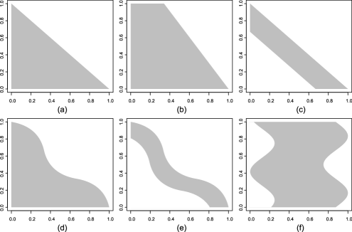
Figure 1: Shapes of possible support sets. The horizontal axis indicates the onset (x) and the vertical the development (y).

The assumptions (A1), (A2), (A5) and (A6) accommodate a variety of sets ${\mathcal{I}}$ that arise in real applications. Figure 1 depicts some realistic examples of the set ${\mathcal{I}}$ that satisfy the assumptions. In particular, those sets of the type in the panels (c) and (e) satisfy (A2) and (A6) if the maximal vertical or horizontal thickness of the stripe is larger than the period $1/J$ of the third component function $f_{3}(m_{J}(\cdot))$. In the interpretation of the examples in Figure 1, we follow the equivalent discussion from Keiding (1991) and Kuang, Nielsen and Nielsen (2008). The triangle in Figure 1(a) is typical for insurance or mortality when none of the underwriting years or cohorts are fully run-off. The standard actuarial term “fully run-off” means that all events from that underwriting year or cohort have been observed. In almost all practical cases of estimating outstanding liabilities, actuaries stick to the triangle format leaving out fully run-off underwriting years. While the triangle also appears in mortality studies, it is common here to leave the fully run-off cohorts in the study resulting in the support shape given in Figure 1(b). The support in Figure 1(c) arises when the data analyst only considers observations from the most recent calendar years. While this approach is omnipresent in practical actuarial science, there is no formal theory or mathematical models behind these procedures in the actuarial literature. This paper is therefore an important step toward formalising mathematically actuarial practise while at the same time improving it. The support given in Figure 1(d) and (e) arises when there is a known time transformation such that time is running at another pace for different underwriting years or cohort years. While this type of time transformations are well known in mortality studies are often coined as versions of accelerated failure time models. Time transformations are also well known in actuarial science coined as operational time. However, the academic literature of actuarial science is still struggling to find a formal definition of what operational time is. This paper offers one potential solution to this outstanding and important issue. The last Figure 1(f) is included to give an impression of the generality of support structures one could deal with inside our model approach. Data is missing in the beginning and end of the delay period, but the model is still valid and in-sample forecasts can be constructed.

The model (1) has taken structured density forecasting into a new territory by leaving the simple multiplicative model. If $f_{3}$ above was constant (and therefore not in the model) then our model reduces to the simple multiplicative model analysed in Martínez-Miranda et al. (2013) and Mammen, Martínez-Miranda and Nielsen (2015). These two papers point out that the simple multiplicative density forecasting model is a continuous version of a widely used parametric approach corresponding to a structured histogram version of in-sample density forecasting based on the simple multiplicative model. The in-sample density forecasting model under investigation in this paper generalizes the simple multiplicative approach in an intuitive and simple way including seasonal effects.

In the following theorem, we show that, if there are two multiplicative representations of the joint density $f$ that agree on almost all points in ${\mathcal{I}}$, then the component functions also agree on almost all points in $[0,1]$. We will use this result later in the asymptotic analysis of our estimation procedure.

Theorem 2.

Assume that model (1) holds with (A1)–(A3), (A5), (A6). Suppose that $(g_{1},g_{2},g_{3})$ is a tuple of functions that are bounded away from zero and infinity with $\int_{0}^{1}g_{1}(x)\,dx=\int_{0}^{1}g_{2}(y)\,dy=1$. Let $\mu_{j}=\log f_{j}-\log g_{j}$. Assume that $\mu_{1}(x)+\mu_{2}(y)+\mu_{3}(m_{J}(x+y))=0$ a.e. on ${\mathcal{I}}$. Then $\mu_{j}\equiv 0$ a.e. on $[0,1]$.

3 Methodology

We describe the estimation method for the model (1). We first note that the marginal densities of $X,Y$ and $m_{J}(X+Y)$ may be zero even if we assume that the joint density is bounded away from zero. For example, the marginal densities of $X$ and $Y$ at the point $u=1$ are zero for the support set ${\mathcal{I}}$ given in Figure 1(a). We estimate the multiplicative density model on a region where we observe sufficient data. This means that we exclude the points $(1,0)$ and $(0,1)$ in the estimation in the case of Figure 1(a), and the point $(1,0)$ in the case of Figure 1(b). Formally, for a set $S\subset{\mathcal{I}}$, let $J_{1}$ and $J_{2}$ denote versions of $I_{1}$ and $I_{2}$, respectively, defined by $J_{1}(y)=\{x\dvtx(x,y)\in S\}$ and $J_{2}(x)=\{y\dvtx(x,y)\in S\}$, and define $J_{3l}(z)=\{x\dvtx(x,(z+l)/J-x)\in S\}$. We take an arbitrarily small number $\delta>0$, and find the largest set $S$ such that

$$\mathrm{mes}\bigl{(}J_{2}(x)\bigr{)} \geq \delta,\qquad\mathrm{mes}\bigl{(}J_{1}(y)\bigr{)}\geq\delta,$$

$$\sum_{l=0}^{L(J)}\mathrm{mes}\bigl{(}J_{3l}\bigl{(}m_{J}(x+y)\bigr{)}\bigr{)} \geq \delta\qquad\mbox{for all }(x,y)\in S,$$

where $\mathrm{mes}(A)$ for a set $A$ denotes its length. Such a set is given by $S=\{(x,y)\dvtx 0\leq x\leq 1-\delta,0\leq y\leq 1-\delta,x+y\leq 1\}$ in the case of Figure 1(a), and $S=\{(x,y)\in{\mathcal{I}}\dvtx 0\leq x\leq 1-\delta\}$ in the case of Figure 1(b), for example.

We estimate $f_{j}$ on $S$. Let $S_{1}$ and $S_{2}$ be the projections of $S$ onto $x$- and $y$-axis, that is, $S_{1}=\{x\in[0,1]\dvtx(x,y)\in S\mbox{ for some }y\in[0,1]\}$, $S_{2}=\{y\in[0,1]\dvtx(x,y)\in S\mbox{ for some }x\in[0,1]\}$, and $S_{3}=\{m_{J}(x+y)\dvtx(x,y)\in S\}$. In the case of Figure 1(a), $S_{1}=S_{2}=[0,1-\delta]$, $S_{3}=[0,1)$, but in the case of Figure 1(b), $S_{1}=[0,1-\delta]$, $S_{2}=[0,1]$, $S_{3}=[0,1)$. We put the following constraints on $f_{j}$:

$$\int_{S_{1}}f_{1}(x)\,dx=\int_{S_{2}}f_{2}(y)=1.$$

This is only for convenience. Now, we define $f_{w,1}(x)=\int_{J_{2}(x)}f(x,y)\,dy,\break f_{w,2}(y)=\int_{J_{1}(y)}f(x,y)\,dx$ and $f_{w,3}(z)=\sum_{l=0}^{L(J)}\int_{J_{3l}(z)}f(x,(z+l)/J-x)\,dx$. Then the model (1) gives the following integral equations:

$$f_{w,1}(x) = f_{1}(x)\int_{J_{2}(x)}f_{2}(y)f_{3}\bigl{(}{{m}_{J}}(x+y)\bigr{)}\,dy,\qquad x\in S_{1},$$

$$f_{w,2}(y) = f_{2}(y)\int_{J_{1}(y)}f_{1}(x)f_{3}\bigl{(}{{m}_{J}}(x+y)\bigr{)}\,dx,\qquad y\in S_{2},$$ (2)

$$f_{w,3}(z) = f_{3}(z)\sum_{l=0}^{L(J)}\int_{J_{3l}(z)}f_{1}(x)f_{2}\bigl{(}(z+l)/J-x\bigr{)}\,dx,\qquad z\in S_{3}.$$

We note that the marginal functions on the left-hand sides of the above equations are bounded away from zero on $S_{j}$. Specifically, $\inf_{u\in S_{j}}f_{w,j}(u)\geq\delta\inf_{(x,y)\in{\mathcal{I}}}f(x,y)>0$ so that $f_{j}$ in the equations are well-defined.

Suppose that we are given a preliminary estimator of the joint density $f$. Call it ${\hat{f}}$. We estimate $f_{w,j}$ by ${\hat{f}}_{w,j}$ that are defined as $f_{w,j}$, respectively, with $f$ being replaced by the preliminary estimator ${\hat{f}}$. Our proposed estimators of $f_{j}$, for $j=1,2,3$, are obtained by replacing $f_{w,j}$ in the integral equations (3) by ${\hat{f}}_{w,j}$, respectively, and solving the resulting equations for the multiplicative components. Let $\vartheta=\int_{S}f(x,y)\,dx\,dy$ and $\hat{\vartheta}$ be its estimator defined by $\hat{\vartheta}=n^{-1}\sum_{i=1}^{n}I[(X_{i},Y_{i})\in S]$. Putting the constraints

$$\int_{S_{1}}{\hat{f}}_{1}(x)\,dx = \int_{S_{2}}{\hat{f}}_{2}(y)\,dy=1,$$

$$\int_{S}{\hat{f}}_{1}(x){\hat{f}}_{2}(y){\hat{f}}_{3}\bigl{(}m_{J}(x+y)\bigr{)}\,dx\,dy = \hat{\vartheta},$$

they are given as the solution of the following backfitting equations:

$${\hat{f}}_{1}(x) = {\hat{\theta}}_{1}\cdot\frac{{\hat{f}}_{w,1}(x)}{\int_{J_{2}(x)}{\hat{f}}_{2}(y){\hat{f}}_{3}({{m}_{J}}(x+y))\,dy},$$

$${\hat{f}}_{2}(y) = {\hat{\theta}}_{2}\cdot\frac{{\hat{f}}_{w,2}(y)}{\int_{J_{1}(y)}{\hat{f}}_{1}(x){\hat{f}}_{3}({{m}_{J}}(x+y))\,dx},$$ (4)

$${\hat{f}}_{3}(z) = {\hat{\theta}}_{3}\cdot\frac{{\hat{f}}_{w,3}(z)}{\sum_{l=0}^{L(J)}\int_{J_{3l}(z)}{\hat{f}}_{1}(x){\hat{f}}_{2}((z+l)/J-x)\,dx},$$

where ${\hat{\theta}}_{j}$ are chosen so that ${\hat{f}}_{j}$ satisfy (3).

The solution of (3) is not given explicitly. The estimates are calculated by an iterative algorithm with a starting set of function estimates ${\hat{f}}_{1}^{[0]}$ and ${\hat{f}}_{2}^{[0]}$ that satisfy the constraints (3). With the initial estimates, we compute ${\hat{f}}_{3}^{[0]}$ from the third equation at (3). Then we update ${\hat{f}}_{j}^{[k-1]}$ consecutively for $j=1,2,3$ and for $k\geq 1$ by the equations at (3) until convergence. Specifically, we compute at the $k$th cycle ($k\geq 1$) of the iteration

$${\hat{f}}_{1}^{[k]}(x) = {\hat{\theta}}_{1}^{[k]}\cdot\frac{{\hat{f}}_{w,1}(x)}{\int_{J_{2}(x)}{\hat{f}}_{2}^{[k-1]}(y){\hat{f}}_{3}^{[k-1]}({{m}_{J}}(x+y))\,dy},$$

$${\hat{f}}_{2}^{[k]}(y) = {\hat{\theta}}_{2}^{[k]}\cdot\frac{{\hat{f}}_{w,2}(y)}{\int_{J_{1}(y)}{\hat{f}}_{1}^{[k]}(x){\hat{f}}_{3}^{[k-1]}({{m}_{J}}(x+y))\,dx},$$ (5)

$${\hat{f}}_{3}^{[k]}(z) = {\hat{\theta}}_{3}^{[k]}\cdot\frac{{\hat{f}}_{w,3}(z)}{\sum_{l=0}^{L(J)}\int_{J_{3l}(z)}{\hat{f}}_{1}^{[k]}(x){\hat{f}}_{2}^{[k]}((z+l)/J-x)\,dx},$$

where ${\hat{\theta}}_{j}^{[k]}$ are chosen so that the resulting ${\hat{f}}_{j}^{[k]}$ satisfy (3).

We note that the naive two-dimensional kernel density estimator is not consistent near the boundary region, which jeopardizes the properties of the solution of the backfitting equation (3) at boundaries. For a preliminary estimator ${\hat{f}}$ of the joint density $f$, we take the local linear estimation technique. The local linear estimator ${\hat{f}}$ we consider here is similar in spirit to the proposal of Cheng (1997). Let ${\mathbf{a}}(u,v;x,y)=(1,(u-x)/h_{1},(v-y)/h_{2})^{\top}$ and define

$$\mathbf{A}(x,y)=\int_{S}{\mathbf{a}}(u,v;x,y){\mathbf{a}}(u,v;x,y)^{\top}h_{1}^{-1}h_{2}^{-1}K\biggl{(}\frac{u-x}{h_{1}}\biggr{)}K\biggl{(}\frac{v-y}{h_{2}}\biggr{)}\,du\,dv,$$

where $(h_{1},h_{2})$ is the bandwidth vector and $K$ is a symmetric univariate probability density function. Also, define

$$\hat{\mathbf{b}}(x,y)=n^{-1}\sum_{i=1}^{n}{\mathbf{a}}(X_{i},Y_{i};x,y)h_{1}^{-1}h_{2}^{-1}K\biggl{(}\frac{X_{i}-x}{h_{1}}\biggr{)}K\biggl{(}\frac{Y_{i}-y}{h_{2}}\biggr{)}W_{i},$$

where $W_{i}=1$ if $(X_{i},Y_{i})\in S$ and $0$ otherwise. The local linear density estimator ${\hat{f}}$ we consider in this paper is defined by $\hat{\eta}_{0}$, where $\hat{\bolds\eta}=(\hat{\eta}_{0},\hat{\eta}_{1},\hat{\eta}_{2})$ is given by

$$\hat{\bolds\eta}(x,y)=\mathbf{A}(x,y)^{-1}\hat{\mathbf{b}}(x,y).$$ (6)

It is alternatively defined as

$$\hat{\bolds\eta}(x,y) = \mathop{\arg\mathrm{min}}_{\bolds\eta}\lim_{b_{1},b_{2}\rightarrow 0}\int_{S}\bigl{[}{\hat{f}}_{b_{1},b_{2}}(u,v)-{\mathbf{a}}(u,v;x,y)^{\top}{\bolds\eta}(x,y)\bigr{]}^{2}$$

$$\hskip 79.0pt{}\times K\biggl{(}\frac{u-x}{h_{1}}\biggr{)}K\biggl{(}\frac{v-y}{h_{2}}\biggr{)}\,du\,dv,$$

where ${\hat{f}}_{b_{1},b_{2}}$ be the standard two-dimensional kernel density estimator defined by

$${\hat{f}}_{b_{1},b_{2}}(x,y)=n^{-1}\sum_{i=1}^{n}b_{1}^{-1}b_{2}^{-1}K\biggl{(}\frac{x-X_{i}}{b_{1}}\biggr{)}K\biggl{(}\frac{y-Y_{i}}{b_{2}}\biggr{)}W_{i}$$

for a bandwidth vector $(b_{1},b_{2})$.

Before we close this section, we give two remarks. One is that, instead of integrating the two-dimensional estimator ${\hat{f}}$, one may estimate $f_{w,j}$ directly from the data. In particular, one may estimate $f_{w,j}$ by the one-dimensional kernel density estimators

$${\tilde{f}}_{w,1}(x) = n^{-1}h_{1}^{-1}\sum_{i=1}^{n}K\biggl{(}\frac{X_{i}-x}{h_{1}}\biggr{)}W_{i},$$

$${\tilde{f}}_{w,2}(y) = n^{-1}h_{2}^{-1}\sum_{i=1}^{n}K\biggl{(}\frac{Y_{i}-y}{h_{2}}\biggr{)}W_{i},$$

$${\tilde{f}}_{w,3}(z) = n^{-1}h_{3}^{-1}\sum_{i=1}^{n}K\biggl{(}\frac{m_{J}(X_{i}+Y_{i})-z}{h_{3}}\biggr{)}W_{i}.$$

Our theory that we present in the next section is valid for this alternative estimation procedure. The other thing we would like to remark is that one may be also interested in an extension of the model (1) that arises when one observes a covariate $\mathbf{U}_{i}\in\mathbb{R}^{d}$ along with $(X_{i},Y_{i})$. A natural extension of the model (1) in this case is that the conditional density of $(X,Y)$ given $\mathbf{U}={\mathbf{u}}$ has the form $f(x,y|{\mathbf{u}})=f_{1}(x,{\mathbf{u}})f_{2}(y,{\mathbf{u}})f_{3}(m_{J}(x+y),{\mathbf{u}}),(x,y)\in{\mathcal{I}}$, where the constraints (B1) now applies to $f_{1}(\cdot,\mathbf{z})$ and $f_{2}(\cdot,\mathbf{z})$ for each $\mathbf{z}$. The method and theory for this extended model are easy to derive from those we present here.

4 Theoretical properties

Let ${\mathcal{S}}$ denote the space of function tuples $\mathbf{g}=(g_{1},g_{2},g_{3})$ with square integrable univariate functions $g_{j}$ in the space $L_{2}[0,1]$. Define nonlinear functionals ${\mathcal{F}}_{j}$ for $1\leq j\leq 3$ on ${\mathcal{S}}$ by

$${\mathcal{F}}_{1}(\mathbf{g}) = 1-\int_{S_{1}}g_{1}(x)\,dx,$$

$${\mathcal{F}}_{2}(\mathbf{g}) = 1-\int_{S_{2}}g_{2}(y)\,dy,$$

$${\mathcal{F}}_{3}(\mathbf{g}) = \vartheta-\int_{S}g_{1}(x)g_{2}(y)g_{3}\bigl{(}{{m}_{J}}(x+y)\bigr{)}\,dx\,dy.$$

Also, define nonlinear functionals ${\mathcal{F}}_{j}$ for $4\leq j\leq 6$, now on $\mathbb{R}^{3}\times{\mathcal{S}}$, by

$${\mathcal{F}}_{4}({\bolds\theta},\mathbf{g})(x) = \int_{J_{2}(x)}\bigl{[}\theta_{1}f(x,y)-g_{1}(x)g_{2}(y)g_{3}\bigl{(}{{m}_{J}}(x+y)\bigr{)}\bigr{]}\,dy,$$

$${\mathcal{F}}_{5}({\bolds\theta},\mathbf{g})(y) = \int_{J_{1}(y)}\bigl{[}\theta_{2}f(x,y)-g_{1}(x)g_{2}(y)g_{3}\bigl{(}{{m}_{J}}(x+y)\bigr{)}\bigr{]}\,dx,$$

$${\mathcal{F}}_{6}({\bolds\theta},\mathbf{g})(z) = \sum_{l=0}^{L(J)}\int_{J_{3l}(z)}\bigl{[}\theta_{3}f\bigl{(}x,(z+l)/J-x\bigr{)}$$

$$\hskip 48.0pt{}-g_{1}(x)g_{2}\bigl{(}(z+l)/J-x\bigr{)}g_{3}(z)\bigr{]}\,dx,$$

where ${\bolds\theta}=(\theta_{1},\theta_{2},\theta_{3})^{\top}$. Then we define a nonlinear operator ${\mathcal{F}}\dvtx\mathbb{R}^{3}\times{\mathcal{S}}\mapsto\mathbb{R}^{3}\times{\mathcal{S}}$ by ${\mathcal{F}}({\bolds\theta},\mathbf{g})(x,y,z)=({\mathcal{F}}_{1}(\mathbf{g}),{\mathcal{F}}_{2}(\mathbf{g}),{\mathcal{F}}_{3}(\mathbf{g}),{\mathcal{F}}_{4}({\bolds\theta},\mathbf{g})(x),{\mathcal{F}}_{5}({\bolds\theta},\mathbf{g})(y),\break{\mathcal{F}}_{6}({\bolds\theta},\mathbf{g})(z))^{\top}$.

Now, we define nonlinear functionals ${\hat{\mathcal{F}}}_{j}$ for $1\leq j\leq 3$ on ${\mathcal{S}}$ and ${\hat{\mathcal{F}}}_{j}$ for $4\leq j\leq 6$ on $\mathbb{R}^{3}\times{\mathcal{S}}$ as ${\mathcal{F}}_{j}$ in the above, with the joint density $f$ being replaced by its estimator ${\hat{f}}$ and $\vartheta$ by $\hat{\vartheta}$. Let ${\hat{\mathcal{F}}}\dvtx\mathbb{R}^{3}\times{\mathcal{S}}\mapsto\mathbb{R}^{3}\times{\mathcal{S}}$ be the nonlinear operator defined by ${\hat{\mathcal{F}}}({\bolds\theta},\mathbf{g})(x,y,z)=({\hat{\mathcal{F}}}_{1}(\mathbf{g}),{\hat{\mathcal{F}}}_{2}(\mathbf{g}),{\hat{\mathcal{F}}}_{3}(\mathbf{g}),{\hat{\mathcal{F}}}_{4}({\bolds\theta},\mathbf{g})(x),{\hat{\mathcal{F}}}_{5}({\bolds\theta},\mathbf{g})(y),\break{\hat{\mathcal{F}}}_{6}({\bolds\theta},\mathbf{g})(z))^{\top}$. Our estimators $\hat{\mathbf{f}}=({\hat{f}}_{1},{\hat{f}}_{2},{\hat{f}}_{3})$ along with $\hat{\bolds\theta}=({\hat{\theta}}_{1},{\hat{\theta}}_{2},{\hat{\theta}}_{3})$ are given as the solution of the equation

$${\hat{\mathcal{F}}}(\hat{\bolds\theta},\hat{\mathbf{f}})={\mathbf{0}}.$$ (7)

From the definition of the nonlinear operator ${\mathcal{F}}$, we also get ${\mathcal{F}}({\mathbf{1}},\mathbf{f})={\mathbf{0}}$, where ${\mathbf{1}}=(1,1,1)^{\top}$ and $\mathbf{f}=(f_{1},f_{2},f_{3})^{\top}$ for the true component functions $f_{j}$.

We consider a theoretical approximation of $\hat{\mathbf{f}}$. Define a nonlinear operator by ${\mathcal{G}}({\bolds\theta},\mathbf{g})={\mathcal{F}}({\mathbf{1}}+{\bolds\theta},\mathbf{f}\circ({\mathbf{1}}+\mathbf{g}))$, where $\mathbf{g}_{1}\circ\mathbf{g}_{2}$ denotes the entry-wise multiplication of the two function vectors $\mathbf{g}_{1}$ and $\mathbf{g}_{2}$. Then ${\mathcal{G}}({\mathbf{0}},{\mathbf{0}})={\mathbf{0}}$. Let ${\mathcal{G}}^{\prime}(\mathbf{d},{\bolds\delta})$ denote the derivative of ${\mathcal{G}}({\bolds\theta},\mathbf{g})$ at $({\bolds\theta},\mathbf{g})=({\mathbf{0}},{\mathbf{0}})$ to the direction $(\mathbf{d},{\bolds\delta})$. We write $\mathbf{f}_{w}(x,y,z)=(f_{w,1}(x),f_{w,2}(y),f_{w,3}(z))^{\top}$ and $\hat{\bolds\mu}(x,y,z)=(\hat{\mu}_{1}(x),\hat{\mu}_{2}(y),\hat{\mu}_{3}(z))^{\top}$, where

$$\hat{\mu}_{1}(x) = f_{w,1}(x)^{-1}\int_{J_{2}(x)}\bigl{[}{\hat{f}}(x,y)-f(x,y)\bigr{]}\,dy,$$

$$\hat{\mu}_{2}(y) = f_{w,2}(y)^{-1}\int_{J_{1}(y)}\bigl{[}{\hat{f}}(x,y)-f(x,y)\bigr{]}\,dx,$$

$$\hat{\mu}_{3}(z) = f_{w,3}(z)^{-1}\sum_{l=0}^{L(J)}\int_{J_{3l}(z)}\bigl{[}{\hat{f}}\bigl{(}x,(z+l)/J-x\bigr{)}$$

$$\hskip 95.0pt{}-f\bigl{(}x,(z+l)/J-x\bigr{)}\bigr{]}\,dx.$$

Let ${\mathcal{G}}^{\prime-1}\dvtx\mathbb{R}^{3}\times{\mathcal{S}}\mapsto\mathbb{R}^{3}\times{\mathcal{S}}$ denote the inverse of ${\mathcal{G}}^{\prime}$, whose existence we will prove in the Appendix. We define ${\bar{\mathbf{f}}}=(\bar{f}_{1},\bar{f}_{2},\bar{f}_{3})$ along with ${\bar{\bolds\theta}}=(\bar{\theta}_{1},\bar{\theta}_{2},\bar{\theta}_{3})$ by

$$\pmatrix{{\bar{\bolds\theta}}-{\mathbf{1}}\cr({\bar{\mathbf{f}}}-\mathbf{f})/\mathbf{f}}={\mathcal{G}}^{\prime-1}\pmatrix{{\mathbf{0}}\cr-\mathbf{f}_{w}\circ\hat{\bolds\mu}},$$ (9)

where $\mathbf{g}_{1}/\mathbf{g}_{2}$ denotes the entrywise division of the function $\mathbf{g}_{1}$ by $\mathbf{g}_{2}$.

It can be seen that ${\bolds\delta}=(\delta_{1},\delta_{2},\delta_{3})^{\top}=((\bar{f}_{1}-f_{1})/f_{1},(\bar{f}_{2}-f_{2})/f_{2},(\bar{f}_{3}-f_{3})/f_{3})^{\top}$ along with $\mathbf{d}=(d_{1},d_{2},d_{3})^{\top}=(\bar{\theta}_{1}-1,\bar{\theta}_{2}-1,\bar{\theta}_{3}-1)^{\top}$ are given as the solution of the following system of integral equations:

$$\delta_{1}(x) = d_{1}+\hat{\mu}_{1}(x)-\int_{J_{2}(x)}\delta_{2}(y)\frac{f(x,y)}{f_{w,1}(x)}\,dy$$ (10)

$${}-\int_{J_{2}(x)}\delta_{3}\bigl{(}{{m}_{J}}(x+y)\bigr{)}\frac{f(x,y)}{f_{w,1}(x)}\,dy,\qquad x\in S_{1},$$

$$\delta_{2}(y) = d_{2}+\hat{\mu}_{2}(y)-\int_{J_{1}(y)}\delta_{1}(x)\frac{f(x,y)}{f_{w,2}(y)}\,dx$$

$${}-\int_{J_{1}(y)}\delta_{3}\bigl{(}{{m}_{J}}(x+y)\bigr{)}\frac{f(x,y)}{f_{w,2}(y)}\,dx,\qquad y\in S_{2},$$

$$\delta_{3}(z) = d_{3}+\hat{\mu}_{3}(z)-\sum_{l=0}^{L(J)}\int_{J_{3l}(z)}\delta_{1}(x)\frac{f(x,(z+l)/J-x)}{f_{w,3}(z)}\,dx$$

$${}-\sum_{l=0}^{L(J)}\int_{J_{3l}(z)}\delta_{2}\bigl{(}(z+l)/J-x\bigr{)}\frac{f(x,(z+l)/J-x)}{f_{w,3}(z)}\,dx,\qquad z\in S_{3},$$

subject to the constraints

$$0 = \int_{S_{1}}f_{1}(x)\delta_{1}(x)\,dx,$$

$$0 = \int_{S_{2}}f_{2}(y)\delta_{2}(y)\,dy,$$ (11)

$$0 = \int_{S}f(x,y)\bigl{[}\delta_{1}(x)+\delta_{2}(y)+\delta_{3}\bigl{(}{{m}_{J}}(x+y)\bigr{)}\bigr{]}\,dx\,dy.$$

In the following theorem, we show that the approximation of $\hat{\mathbf{f}}$ by ${\bar{\mathbf{f}}}$ is good enough. In the theorem, we assume that ${\hat{f}}(x,y)-f(x,y)=O_{p}(\varepsilon_{n})$ uniformly on $S$ for some nonnegative sequence $\{\varepsilon_{n}\}$ that converges to zero as $n$ tends to infinity. For the local linear estimator ${\hat{f}}$ defined by (6) with $h_{1}\sim h_{2}\sim n^{-1/5}$, we have $\varepsilon_{n}=n^{-3/10}\sqrt{\log n}$. The theorem tells that the approximation errors of $\bar{f}_{j}$ for ${\hat{f}}_{j}$ are of order $O_{p}(n^{-3/5}\log n)$. In Theorem 4 below, we will show that $\bar{f}_{j}-f_{j}$ have magnitude of order $O_{p}(n^{-2/5}\sqrt{\log n})$ uniformly on $S_{j}$. This means that the first-order properties of ${\hat{f}}_{j}$ are the same as those of $\bar{f}_{j}$.

Theorem 3.

Assume that the conditions of Theorem 2 hold, and that the joint density $f$ is bounded away from zero and infinity on its support $S$ with continuous partial derivatives on the interior of $S$. If ${\hat{f}}(x,y)-f(x,y)=O_{p}(\varepsilon_{n})$ uniformly for $(x,y)\in S$, then it holds that $|\hat{\theta}_{j}-\bar{\theta}_{j}|=O_{p}(\varepsilon_{n}^{2})$ and $\sup_{u\in S_{j}}|{\hat{f}}_{j}(u)-\bar{f}_{j}(u)|=O_{p}(\varepsilon_{n}^{2})$.

Next, we present the limit distribution of $({\bar{\mathbf{f}}}-\mathbf{f})/\mathbf{f}$. In the next theorem, we assume that $h_{1}\sim c_{1}n^{-1/5}$ and $h_{2}\sim c_{2}n^{-1/5}$ for some constants $c_{1},c_{2}>0$. For such constants, define

$${\tilde{f}}^{B}(x,y)=\frac{1}{2}\int u^{2}K(u)\,du\biggl{[}c_{1}^{2}\frac{\partial^{2}}{\partial x^{2}}f(x,y)+c_{2}^{2}\frac{\partial^{2}}{\partial y^{2}}f(x,y)\biggr{]}.$$ (12)

Also, define ${\tilde{\mu}}_{j}^{B}$ for $j=1,2,3$ as $\hat{\mu}_{j}$ at (4) with the local linear estimator ${\hat{f}}$ being replaced by ${\tilde{f}}^{B}$. In the Appendix, we will show that the asymptotic mean of $(\bar{f}_{j}-f_{j})/f_{j}$ equals $n^{-2/5}\beta_{j}$, where ${\bolds\beta}=(\beta_{1},\beta_{2},\beta_{3})$ is the solution of the backfitting equation (10) with $\hat{\bolds\mu}$ being replaced by $\tilde{\bolds\mu}^{B}$. Let ${\tilde{f}}^{A}$ denote the centered version of the naive two-dimensional kernel density estimator. Specifically,

$${\tilde{f}}^{A}(x,y)=n^{-1}\sum_{i=1}^{n}\bigl{[}K_{h_{1}}(X_{i}-x)K_{h_{2}}(Y_{i}-y)$$

(13)

$$\hskip 66.0pt\qquad{}-E\bigl{(}K_{h_{1}}(X_{i}-x)K_{h_{2}}(Y_{i}-y)\bigr{)}\bigr{]}.$$

Here and below, we write $K_{h}(u)=K(u/h)/h$. Define ${\tilde{\mu}}_{j}^{A}$ for $j=1,2,3$ as ${\tilde{\mu}}_{j}^{B}$ with ${\tilde{f}}^{A}$ taking the role of ${\tilde{f}}^{B}$. We will also show that the asymptotic variances of $(\bar{f}_{j}-f_{j})/f_{j}$ equal those of ${\tilde{\mu}}_{j}^{A}$, respectively, and that they are given by $n^{-4/5}\sigma_{j}^{2}$, where

$$\sigma_{1}^{2}(x) = c_{1}^{-1}f_{w,1}(x)^{-1}\int K^{2}(u)\,du,$$

$$\sigma_{2}^{2}(y) = c_{2}^{-1}f_{w,2}(y)^{-1}\int K^{2}(u)\,du,$$

$$\sigma_{3}^{2}(z) = c_{2}^{-1}f_{w,3}(z)^{-1}\int\bigl{[}K*K(u)\bigr{]}\bigl{[}K*K(c_{1}u/c_{2})\bigr{]}\,du$$

$$= c_{1}^{-1}f_{w,3}(z)^{-1}\int\bigl{[}K*K(u)\bigr{]}\bigl{[}K*K(c_{2}u/c_{1})\bigr{]}\,du,$$

where $K*K$ denotes the two-fold convolution of the kernel $K$.

In the discussion of assumption (A6) in Section 2, we note that (A6) allows a finite number of jumps in $I_{j}(u)$ for $j=1,2$ and $I_{3l}(u)$ as $u$ changes. These jump points are actually those where the marginal densities $f_{w,j}$ are discontinuous. At these discontinuity points, the expression of the asymptotic distributions of the estimators is complicate. For this reason, we consider only those points in the partitions $(a_{k-1}^{j},a_{k}^{j}),1\leq k\leq L_{j}$, for the asymptotic distribution of ${\hat{f}}_{j}$, where $a_{k}^{j}$ are the points that appear in assumption (A6). We denote by $S_{j,c}$ the resulting subset of $S_{j}$ after deleting all $a_{k}^{j},1\leq k\leq L_{j}-1$. Note that $f_{w,j}$ is continuous on $S_{j,c}$ due to (A6). In the theorem below, we also denote by $S_{j}^{\mathrm{o}}$ the interiors of $S_{j}$, $j=1,2,3$.

For the limit distribution of ${\hat{f}}_{j}$, we put an additional condition on the support set. To state the condition, let $J_{2}^{\mathrm{o}}(u_{1};h_{2})$ be a subset of $J_{2}(u_{1})$ such that $v\in J_{2}^{\mathrm{o}}(u_{1};h_{2})$ if and only if $v-h_{2}t\in J_{2}(u_{1})$ for all $t\in[-1,1]$. The set $J_{2}^{\mathrm{o}}(u_{1};h_{2})$ is inside $J_{2}(u_{1})$ at a depth $h_{2}$. In the following assumption, $a_{k}^{j}$ and $\kappa$ are the points and the function that appear in assumption (A6). [(A7)]

There exist constants $C>0$ and $\alpha>1/2$ such that the following statements hold: (i) for any sequence of positive numbers $\varepsilon_{n}$, $J_{2}^{\mathrm{o}}(u_{1};C\varepsilon_{n}^{\alpha})\subset J_{2}(u_{2})$ for all $u_{1},u_{2}\in(a_{k-1}^{1},a_{k}^{1})\cap S_{1}$ with $|u_{1}-u_{2}|\leq\varepsilon_{n}$, $1\leq k\leq L_{1}$; $J_{1}^{\mathrm{o}}(u_{1};\break C\varepsilon_{n}^{\alpha})\subset J_{1}(u_{2})$ for all $u_{1},u_{2}\in(a_{k-1}^{2},a_{k}^{2})\cap S_{2}$ with $|u_{1}-u_{2}|\leq\varepsilon_{n}$, $1\leq k\leq L_{2}$; (ii) $\kappa(t)\leq C|t|^{\alpha}$.

Theorem 4.

Assume that (A7) and the conditions of Theorem 3 hold, and that the joint density $f$ is twice partially continuously differentiable. Let the kernel $K$ be supported on $[-1,1]$, symmetric and Lipschitz continuous. Let the bandwidths $h_{j}$ satisfy $n^{1/5}h_{j}\rightarrow c_{j}$ for some constants $c_{j}>0$. Then, for fixed points $u_{j}\in S_{j}^{\mathrm{o}}\cap S_{j,c}$, it holds that $n^{2/5}(\bar{f}_{j}(u_{j})-f_{j}(u_{j}))/f_{j}(u_{j})$ are jointly asymptotically normal with mean $(\beta_{j}(u_{j})\dvtx 1\leq j\leq 3)$ and variance $\operatorname{diag}(\sigma^{2}_{j}(u_{j})\dvtx 1\leq j\leq 3)$. Furthermore, $(\bar{f}_{j}(u_{j})-f_{j}(u_{j}))/f_{j}(u_{j})=\break O_{p}(n^{-2/5}\sqrt{\log n})$ uniformly for $u_{j}\in S_{j}$.

Remark 2.

In the case where the third component function $f_{3}$ is constant, that is, there is no periodic component, the above theorem continue to hold for the component $f_{1}$ and $f_{2}$ without those conditions that pertain to the set $S_{3}$ and the function $f_{3}$.

5 Numerical properties

5.1 Simulation studies

We considered two densities on ${\mathcal{I}}=\{(x,y)\dvtx 0\leq x,y\leq 1,x+y\leq 1\}$. Model 1 has the components $f_{1}\equiv f_{2}\equiv 1$ on $[0,1]$, and $f_{3}(u)=c_{1}(\sin(2\pi u)+3/2),u\in[0,1]$, where $c_{1}>0$ is chosen to make $f(x,y)=f_{1}(x)f_{2}(y)f_{3}({{m}_{J}}(x+y))$ be a density on ${\mathcal{I}}$. Model 2 has $f_{1}(u)=3/2-u,f_{2}(u)=5/4-3u^{2}/4$ and $f_{3}(u)=c_{2}(u^{3}-3u^{2}/2+u/2+1/2)$ for some constant $c_{2}>0$. We took $J=2$. We computed our estimates on a grid of bandwidth choice $h_{1}=h_{2}$. For model 1, we took $\{0.070+0.001\times j\dvtx 0\leq j\leq 30\}$ in the range $[0.070,0.100]$, and for model 2 we chose $\{0.40+0.02\times j\dvtx 0\leq j\leq 20\}$ in the range $[0.40,0.80]$. In both cases, the ranges covered the optimal bandwidths. We obtained $\mathrm{MISE}_{j}=E\int_{0}^{1}[\hat{f}_{j}(u)-f_{j}(u)]^{2}\,du$, $\mathrm{ISB}_{j}=\int_{0}^{1}[E\hat{f}_{j}(u)-f_{j}(u)]^{2}\,du$ and $\mathrm{IV}_{j}=E\int_{0}^{1}[\hat{f}_{j}(u)-E\hat{f}_{j}(u)]^{2}\,du$, for $1\leq j\leq 3$, based on 100 pseudo samples. The sample sizes were $n=400$ and $1000$, but only the results for $n=400$ are reported since the lessons are the same.

Figure 2 is for model 1. It shows the boxplots of the values of $\mathrm{MISE}_{j}$, $\mathrm{ISB}_{j}$ and $\mathrm{IV}_{j}$ computed using the bandwidths on the grid specified above, and thus gives some indication of how sensitive our estimators are to the choice of bandwidth. The bandwidth that gave the minimal value of $\mathrm{MISE}_{1}+\mathrm{MISE}_{2}+\mathrm{MISE}_{3}$ was $h_{1}=h_{2}=0.089$ in model 1, and $h_{1}=h_{2}=0.64$ in model 2, for the sample size $n=400$. The values of $\mathrm{MISE}_{j}$ along with $\mathrm{ISB}_{j}$ and $\mathrm{IV}_{j}$ for these optimal bandwidths are reported in Table 1. Although our primary concern is the estimation of the component functions, it is also of interest to see how good the produced two-dimensional density estimator $\hat{f}_{1}(x)\hat{f}_{2}(y)\hat{f}_{3}({{m}_{J}}(x+y))$ behaves. For this, we include in the table the values of MISE, ISB and IV of the two-dimensional estimates computed using the optimal bandwidth $h_{1}=h_{2}=0.089$ in model 1, and $h_{1}=h_{2}=0.64$ in model 2. For comparison, we also report the results for the two-dimensional local linear estimates defined at (6). For the local linear estimator, we used its optimal choices $h_{1}=h_{2}=0.085$ in model 1, and $h_{1}=h_{2}=0.48$ in model 2. We found that the initial local linear estimates had a large portion of mass outside ${\mathcal{I}}$, and thus behaved very poorly if they were not re-scaled to be integrated to one on ${\mathcal{I}}$. The reported values in Table 1 are for the adjusted local linear estimates. Overall, our two-dimensional estimator has better performance than the local linear estimator, especially in model 2. Figure 3 depicts the true density of model 1 and our two-dimensional estimate that has the median performance in terms of ISE.

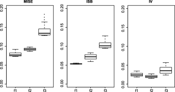
Figure 2: Boxplots for the values of MISE, ISB and IV of our estimates $f_{j}$ computed using various bandwidth choices (model 1, $n=400$).

Table 1: Mean integrated squared errors (MISE), integrated squared biases (ISB) and integrated variance (IV) of the estimators

		Component functions			Joint density
		$\bolds{f_{1}}$	$\bolds{f_{2}}$	$\bolds{f_{3}}$	Our est.	Local linear
Model 1	MISE	0.0756	0.0937	0.1283	0.2493	0.2537
	ISB	0.0528	0.0752	0.0963	0.1844	0.2199
	IV	0.0228	0.0184	0.0320	0.0649	0.0338
Model 2	MISE	0.0124	0.0057	0.0130	0.0475	0.0624
	ISB	0.0120	0.0054	0.0127	0.0469	0.0607
	IV	0.0004	0.0003	0.0003	0.0006	0.0017

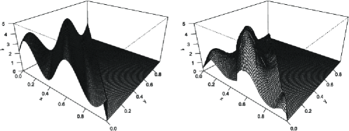
Figure 3: The true density (left) and our estimated two-dimensional density function (right) computed from the pseudo sample that gives the median performance in terms of ISE, for model 1 and $n=400$.

5.2 Data examples

The original data set we analyze in this section was collected between the year 1990 to 2011 by the major global UK based nonlife insurance company RSA. The dataset—and more details about it—is publicly available via the Cass Business School web site together with the paper “Double Chain Ladder” at the Cass knowledge site. The observations were the incurred counts of large claims aggregated by months. During the 264 months, 1516 large claims were made. The dataset is provided in the form of a classical run-off triangle $\{N_{kl}\dvtx 1\leq k,l\leq 264,k+l\leq 265\}$, where $N_{kl}$ denotes the number of large claims incurred in the $k$th month and reported in the $(k+l-1)$th month, that is, with $(l-1)$ months delay. Since the data are grouped monthly, we need pre-smoothing of the data to apply the model (1) that is based on data recorded over a continuous time scale. A natural way of pre-smoothing is to perturb the data by uniform random variables. Thus, we converted each claim $(k,l)$ on the two-dimensional discrete time scale $\{(k,l)\dvtx 1\leq k,l\leq 264,k+l\leq 265\}$, into $(X,Y)$ on the two-dimensional continuous time scale ${\mathcal{I}}=\{(x,y)\dvtx 0\leq x,y\leq 1,x+y\leq 1\}$, by

$$X=\frac{k-1+U_{1}}{264},\qquad Y=\frac{l-1+U_{2}}{264},$$

where $(U_{1},U_{2})$ is a two-dimensional uniform random variate on the unit square $[0,1]^{2}$. This gives a converted dataset $\{(X_{i},Y_{i})\dvtx 1\leq i\leq 1516\}$. We applied to this dataset our method of estimating the structured density $f$ of $(X,Y)$.

Since one month corresponds to an interval with length $1/264$ on the $[0,1]$ scale, one year is equivalent to an interval with length $12/264=1/22$ on the latter scale. We let the periodic component $f_{3}(m_{J}(\cdot))$ in the model (1) reflect a possible seasonal effect, so that we take one year in the real time to be the period of the function. This means that we let the periodic component $f_{3}(m_{J}(\cdot))$ have $1/22$ as its period, and thus take $J=22$. For the bandwidth, we took $h_{1}=h_{2}=0.01$. The chosen bandwidth may be considered to be too small for the estimation of $f_{1}$ and $f_{2}$. However, we took such a small bandwidth to detect possible seasonality. Note that the bandwidth size $0.01$ corresponds to $0.01\times 12\times 22=2.64$ months. We found that even with this small bandwidth the estimated curve ${\hat{f}}_{3}$ was nearly a constant function, which suggests that the large claim data do not have a seasonal effect.

To see how well our method detects a possible seasonal effect in the data, we augmented the dataset by adding a certain level of seasonal effect as follows. We computed

$$N_{kl}^{\prime} = 2N_{kl}\qquad\mbox{if }k+l=12m\mbox{ for some }m=1,2,\ldots,$$

$$N_{kl}^{\prime} = 3N_{kl}\qquad\mbox{if }k+l=12m+1\mbox{ for some }m=1,2,\ldots,$$

$$N_{kl}^{\prime} = 5N_{kl}\qquad\mbox{if }k+l=12m+2\mbox{ for some }m=0,1,\ldots,$$

$$N_{kl}^{\prime} = 3N_{kl}\qquad\mbox{if }k+l=12m+3\mbox{ for some }m=0,1,\ldots,$$

$$N_{kl}^{\prime} = N_{kl}\qquad\mbox{otherwise}.$$

Since ($k+l-1$ modulo $12$) is the actual month of the claims reported, the augmented dataset has added claims in November, December, January and February. The augmentation resulted in increasing the total number of claims to 2606 from 1516. The increased counts of reported claims were 252 from 126 for November, 600 from 200 for December, 455 from 91 for January and 300 from 100 for February.

In our estimation procedure, the bandwidths $h_{1}$ and $h_{2}$ control the smoothness of the local linear estimate $\hat{f}$ along the $x$- and $y$-axis, respectively. Consequently, choosing small values for $h_{1}$ and $h_{2}$ would result in nonsmooth estimates of the functions $f_{1}$ and $f_{2}$, which we observed in the pilot study with $h_{1}=h_{2}=0.01$. Nevertheless, in some cases setting these bandwidths to be small, relative to the scales of $X$ and $Y$, might be preferred when one needs to detect possible seasonality, as is the case with the current dataset. In our dataset, the bandwidth size $1/264=0.0038$ on the scale of $[0,1]$ corresponds to one month in real time. Thus, taking the bandwidths to be $0.015$, for example, that corresponds to a period of four months, forces the seasonal effect to almost vanish in the estimate of $f_{3}$.

To achieve both aims of producing smooth estimates of $f_{1}$ and $f_{2}$, and of detecting possible seasonal effect, we applied to the augmented dataset a two-stage procedure that is based on our estimation method described in Section 3. In the first stage, we got a local linear estimate $\hat{f}$ with $h_{1}=h_{2}=0.01$, and found an estimate of $f_{3}$ using the iteration scheme at (3). In the second stage, we recomputed a local linear estimate $\hat{f}$ with larger bandwidths $h_{1}=h_{2}=0.05$, and found estimates of $f_{1}$ and $f_{2}$ using only the first two updating equations at (3) with $\hat{f}_{3}^{[k-1]}$ being replaced by the estimate of $f_{3}$ obtained in the first stage.

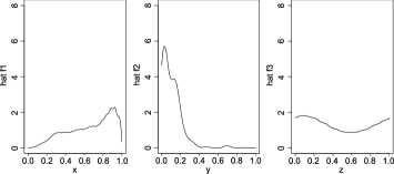
Figure 4: Estimated curves $\hat{f}_{j}$ for the model (1) obtained by applying the two-stage procedure to the augmented large claim data.

The results of applying this two-stage procedure to the augmented dataset are presented in Figure 4. Clearly, the seasonal effect of the augmented dataset was well recovered in the estimate of $f_{3}$, and at the same time smooth estimates of $f_{1}$ and $f_{2}$ were produced. The augmented data set indicate an increased number of claims in the winter time. This is clearly reflected in the estimated results, where the first part and the last part of the estimated effect is higher than the rest of the curve. Imagine the realistic situation that a nonlife insurer on the first day of November has to produce budget expenses for the rest of the year. The classical multiplicative methodology is not able to reflect the two month perspective of such a budget. Therefore, considerable work is being done manually in finance and actuarial departments of nonlife insurance companies to correct for such effects. With our new seasonal correction, costly manual procedures can be replaced by cost saving automatic ones eventually benefitting the prices all of us as end customers have to pay for insurance products.

Figure 5 depicts the resulting two-dimensional joint density. Notice that this two-dimensional density is clearly nonmultiplicative. The seasonal correction provides a visually deviation from the multiplicative shape. Also, note that while this two-dimensional density is nonmultiplicative, the nature of this deviation is not immediately clear to the eye. Whether the deviation is pure noise, a seasonal effect or some other effect is not easy to get from the full two-dimensional graph of the local linear density estimate which is also presented in Figure 5. For the local linear estimate, we used $h_{1}=h_{2}=0.03$. We tried other bandwidth choices such as $0.01$ and $0.05$, but found that the smaller one gave too rough estimate and the larger one produced too smooth a surface. Our two-dimensional density estimate therefore illustrates why research into structured densities on nontrivial supports is crucial to extract information beyond the classical and simple multiplicative one.

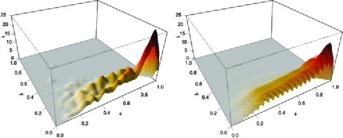
Figure 5: Local linear joint density estimate (left) and our estimate (right) for the model (1) obtained by applying the two-stage procedure to the augmented large claim data.

Appendix

.3 Proof of Theorem 1

Suppose that $(g_{1},g_{2},g_{3})$ is a tuple of functions that are bounded away from zero and infinity with $\int_{0}^{1}g_{1}(x)\,dx=\int_{0}^{1}g_{2}(y)\,dy=1$ and

$$f(x,y)=g_{1}(x)g_{2}(y)g_{3}\bigl{(}{{m}_{J}}(x+y)\bigr{)}.$$

Furthermore, we assume that $g_{1}$ and $g_{2}$ are differentiable on $[0,1]$ and that $g_{3}$ is twice differentiable on $[0,1)$. For $j\in\{1,2,3\}$ define $\mu_{j}=\log f_{j}-\log g_{j}$. By assumption, we have

$$\mu_{1}(x)+\mu_{2}(y)+\mu_{3}\bigl{(}m_{J}(x+y)\bigr{)}=0.$$

For $z\in[0,1)$, we choose $(x,y)$ in the interior of ${\mathcal{I}}$ with $m_{J}(x+y)=z$. Then we have that

$$0={\partial^{2}\over\partial x\,\partial y}\bigl{[}\mu_{1}(x)+\mu_{2}(y)+\mu_{3}\bigl{(}m_{J}(x+y)\bigr{)}\bigr{]}=\mu_{3}^{\prime\prime}(z).$$

Thus, $\mu_{3}$ is a linear function. Furthermore, we have that $\mu_{3}(0)=\mu_{3}(1-)$. This follows by noting that $\mu_{3}(0)=-\mu_{1}(x)-\mu_{2}(y)$ for $(x,y)\in{\mathcal{I}}$ with $m_{J}(x+y)=0$. Note that $m_{J}(x+y)=0$ if and only if $x+y=l/J$ for some $l\geq 1$, if $(x,y)$ is in the interior of ${\mathcal{I}}$. After slightly decreasing $x$ and $y$ to $x+\delta_{x}$ and $y+\delta_{y}$ with small $\delta_{x}<0$, $\delta_{y}<0$, we have that $\mu_{3}(1+J(\delta_{x}+\delta_{y}))=-\mu_{1}(x+\delta_{x})-\mu_{2}(y+\delta_{y})$ since $m_{J}(x+y+\delta_{x}+\delta_{y})=1+J(\delta_{x}+\delta_{y})$. Thus, $\mu_{3}(0)=\mu_{3}(1-)$ follows from continuity of $\mu_{1}$ and $\mu_{2}$. We conclude that $\mu_{3}$ must be a constant function. Thus, $\mu_{1}(x)+\mu_{2}(y)$ is a constant function.

From assumption (A5), we get that $\mu_{1}(x)$ is constant on the intervals $[x_{j},x_{j+1}]$. Because the union of these intervals is equal to $[0,1]$ we conclude that $\mu_{1}(x)$ is constant on $[0,1]$. Using again (A5) we get that $\mu_{2}(y)$ is constant on $[0,1]$. Because of the assumption that $\int_{0}^{1}g_{1}(x)\,dx=\int_{0}^{1}g_{2}(y)\,dy=1$ and $\int_{0}^{1}f_{1}(x)\,dx=\int_{0}^{1}f_{2}(y)\,dy=1$ we get that $f_{1}=g_{1}$, $f_{2}=g_{2}$ and $f_{3}=g_{3}$. This completes the proof.

.4 Proof of Theorem 2

We first argue that $\mu_{1}$, $\mu_{2}$ and $\mu_{3}$ are a.e. equal to piecewise continuous functions on $(0,1)$, with a finite number of pieces. To see that $\mu_{1}$ is a.e. equal to a piecewise continuous function, we note that

$$\mu_{1}(x)=-\int_{I_{2}(x)}\bigl{[}\mu_{2}(y)+\mu_{3}\bigl{(}m_{J}(x+y)\bigr{)}\bigr{]}\,dy/\mathrm{mes}\bigl{(}I_{2}(x)\bigr{)}\qquad\mbox{a.e. }x\in(0,1).$$

Here, because of (A3) and (A6), the right-hand side is a piecewise continuous function. Thus, $\mu_{1}$ is a.e. equal to a piecewise continuous function. In abuse of notation, we now denote the piecewise continuous function by $\mu_{1}$. By similar arguments, one sees that $\mu_{2}$, and $\mu_{3}$ are piecewise continuous functions (or more precisely a.e. equal to piecewise continuous functions). This implies that

$$\mu_{1}(x)+\mu_{2}(y)+\mu_{3}\bigl{(}m_{J}(x+y)\bigr{)}=0$$ (14)

for $(x,y,m_{J}(x+y))\notin\{x_{1},\ldots,x_{r_{1}}\}\times(0,1)^{2}\cup(0,1)\times\{y_{1},\ldots,y_{r_{2}}\}\times(0,1)\cup(0,1)^{2}\times\{z_{1},\ldots,z_{r_{3}}\}$ for some values $x_{1},\ldots,x_{r_{1}},y_{1},\ldots,y_{r_{2}},z_{1},\ldots,z_{r_{3}}\in(0,1)$.

We now argue that $\mu_{3}$ is continuous on $[0,1)$. To see that $\mu_{3}$ is continuous at $z_{0}\in[0,1)$, we choose $(x_{0},y_{0})$ in the interior of ${\mathcal{I}}$ such that $m_{J}(x_{0}+y_{0})=z_{0}$. This is possible because of assumption (A2). We can choose $x_{0}$ and $y_{0}$ such that $\mu_{1}$ is continuous at $x_{0}$ and $\mu_{2}$ is continuous at $y_{0}$. Thus, we get from (14) that $\mu_{3}$ is continuous at $z_{0}$. Similarly, one shows that $\mu_{1}$ and $\mu_{2}$ are continuous functions on $[0,1]$. This gives that

$$\mu_{1}(x)+\mu_{2}(y)+\mu_{3}\bigl{(}m_{J}(x+y)\bigr{)}=0$$ (15)

for all $x,y\in(0,1)$.

For $z_{0}\in[0,1)$, we choose $(x_{0},y_{0})$ in the interior of ${\mathcal{I}}$ with $m_{J}(x_{0}+y_{0})=z_{0}$. Note that for $\delta_{x}$ and $\delta_{y}$ sufficiently small we get for $z_{0}\in(0,1)$ that $m_{J}(x_{0}+\delta_{x}+y_{0}+\delta_{y})=z_{0}+J(\delta_{x}+\delta_{y})$. This gives for $\delta_{x}$ and $\delta_{y}$ sufficiently small that

$$\mu_{1}(x_{0}+\delta_{x})+\mu_{2}(y_{0}+\delta_{y})+\mu_{3}\bigl{(}z_{0}+J(\delta_{x}+\delta_{y})\bigr{)}=0.$$

With $\delta_{x}$, $\delta_{y}^{\prime}$ and $\delta_{y}$ sufficiently small, we get that

$$\mu_{2}(y_{0}+\delta_{y})+\mu_{3}\bigl{(}z_{0}+J(\delta_{x}+\delta_{y})\bigr{)}=\mu_{2}\bigl{(}y_{0}+\delta_{y}^{\prime}\bigr{)}+\mu_{3}\bigl{(}z_{0}+J\bigl{(}\delta_{x}+\delta_{y}^{\prime}\bigr{)}\bigr{)}.$$

With the special choice $\delta_{x}=-\delta_{y}$, this gives

$$\mu_{2}(y_{0}+\delta_{y})+\mu_{3}(z_{0})=\mu_{2}\bigl{(}y_{0}+\delta_{y}^{\prime}\bigr{)}+\mu_{3}\bigl{(}z_{0}+J\bigl{(}\delta_{y}^{\prime}-\delta_{y}\bigr{)}\bigr{)}.$$

Let $\gamma$ be a function defined by $\gamma(u)=\mu_{3}(z_{0}+Ju)-\mu_{3}(z_{0})$. From the last two equations taking $u=\delta_{x}+\delta_{y}$ and $v=\delta_{y}^{\prime}-\delta_{y}$, we get

$$\gamma(u+v)=\gamma(u)+\gamma(v)$$

for $u,v$ sufficiently small. This implies that, with a constant $c_{z_{0}}$ depending on $z_{0}$ we have $\gamma(u)=c_{z_{0}}u$ for $u$ sufficiently small; see Theorem 3 of Guillot, Khare and Rajaratnam (2013). Thus, we obtain $\mu_{3}(z)=a_{z_{0}}+b_{z_{0}}z$ with constants $a_{z_{0}}$ and $b_{z_{0}}$ depending on $z_{0}$ for $z$ in a neighborhood $U_{z_{0}}$ of $z_{0}$. Because every interval $[z^{\prime},z^{\prime\prime}]$ with $0<z^{\prime}<z^{\prime\prime}<1$ can be covered by the union of finitely many $U_{z}$’s we get that for each such interval it holds that $\mu_{3}(z)=a_{z^{\prime},z^{\prime\prime}}+b_{z^{\prime},z^{\prime\prime}}z$ for $z\in[z^{\prime},z^{\prime\prime}]$ with constants $a_{z^{\prime},z^{\prime\prime}}$ and $b_{z^{\prime},z^{\prime\prime}}$ depending on the chosen interval $[z^{\prime},z^{\prime\prime}]$.

One can repeat the above arguments for $z_{0}=0$. Then we have that $m_{J}(x_{0}+\delta_{x}+y_{0}+\delta_{y})=1+J(\delta_{x}+\delta_{y})$ for $\delta_{x}+\delta_{y}<0$ and $m_{J}(x_{0}+\delta_{x}+y_{0}+\delta_{y})=J(\delta_{x}+\delta_{y})$ for $\delta_{x}+\delta_{y}>0$. Arguing as above with $\delta_{x}+\delta_{y}>0$ and $\delta_{y}^{\prime}-\delta_{y}>0$ we get that $\mu_{3}(z)=a_{+}+b_{+}z$ for $z\in(0,z^{+}]$ for $z^{+}>0$ small enough with some constants $a_{+}$ and $b_{+}$. Similarly, we get by choosing $\delta_{x}+\delta_{y}<0$ and $\delta_{y}^{\prime}-\delta_{y}<0$ that $\mu_{3}(z)=a_{-}+b_{-}z$ for $z\in(z^{-},1)$ for $z^{-}<1$ large enough with some constants $a_{-}$ and $b_{-}$. Thus, we get that $\mu_{3}(z)=a+bz$ for $z\in(0,1)$ with some constants $a$ and $b$.

Furthermore, using continuity of $\mu_{1}$, $\mu_{2}$ and the relation $\mu_{3}(m_{J}(x+y))=-\mu_{1}(x)-\mu_{2}(y)$ for $z=m_{J}(x+y)$ with $z$ in $(1-\delta,1)$ and $(0,\delta)$ with $\delta>0$ small enough we get that $\mu_{3}(0)=\mu_{3}(1-)$. Thus, we have $b=0$ and we conclude that $\mu_{3}$ is a constant function. This gives

$$\mu_{1}(x)+\mu_{2}(y)=-a$$

for all $(x,y)\in{\mathcal{I}}$. Now arguing as in the proof of Theorem 1 we get that $f_{1}=g_{1}$, $f_{2}=g_{2}$ and $f_{3}=g_{3}$. This completes the proof.

.5 Proof of Theorem 3

Let ${\mathcal{G}}^{\prime}({\bolds\theta},\mathbf{g})(\mathbf{d},{\bolds\delta})$ denote the derivative ${\mathcal{G}}$, defined in Section 4, at $({\bolds\theta},\mathbf{g})$ to the direction $(\mathbf{d},{\bolds\delta})$. We note that we write ${\mathcal{G}}^{\prime}({\mathbf{0}},{\mathbf{0}})(\mathbf{d},{\bolds\delta})$ simply as ${\mathcal{G}}^{\prime}(\mathbf{d},{\bolds\delta})$ in Section 4. We use the sup-norm $\|(\mathbf{d},{\bolds\delta})\|_{\infty}$ as a metric in the space $\mathbb{R}^{3}\times{\mathcal{S}}$, defined by

$$\bigl{\|}(\mathbf{d},{\bolds\delta})\bigr{\|}_{\infty}=\max\Bigl{\{}|d_{1}|,|d_{2}|,|d_{3}|,\sup_{u\in S_{1}}\bigl{|}\delta_{1}(u)\bigr{|},\sup_{u\in S_{2}}\bigl{|}\delta_{2}(u)\bigr{|},\sup_{u\in S_{3}}\bigl{|}\delta_{3}(u)\bigr{|}\Bigr{\}}.$$

Define ${\hat{\mathcal{G}}}({\bolds\theta},\mathbf{g})={\hat{\mathcal{F}}}({\mathbf{1}}+{\bolds\theta},\mathbf{f}\circ({\mathbf{1}}+\mathbf{g}))$, where ${\hat{\mathcal{F}}}$ is defined in Section 4, and let ${\hat{\mathcal{G}}}^{\prime}({\bolds\theta},\mathbf{g})$ denote the derivative of ${\hat{\mathcal{G}}}$ at $({\bolds\theta},\mathbf{g})$. In the setting where ${\hat{f}}(x,y)-f(x,y)=O_{p}(\varepsilon_{n})$ uniformly for $(x,y)\in{\mathcal{I}}$, we claim: [(iii)]

$\sup_{\|(\mathbf{d},{\bolds\delta})\|_{\infty}=1}\|{\hat{\mathcal{G}}}^{\prime}({\mathbf{0}},{\mathbf{0}})(\mathbf{d},{\bolds\delta})-{\mathcal{G}}^{\prime}({\mathbf{0}},{\mathbf{0}})(\mathbf{d},{\bolds\delta})\|_{\infty}=O_{p}(\varepsilon_{n})$;

The operator ${\mathcal{G}}^{\prime}({\mathbf{0}},{\mathbf{0}})$ is invertible and has bounded inverse;

The operator ${\hat{\mathcal{G}}}^{\prime}$ is Lipschitz continuous with probability tending to one, that is, there exists constants $r,C>0$ such that, with probability tending to one,

$$\sup_{\|(\mathbf{d},{\bolds\delta})\|_{\infty}=1}\bigl{\|}{\hat{\mathcal{G}}}^{\prime}({\bolds\theta}_{1},\mathbf{g}_{1})(\mathbf{d},{\bolds\delta})-{\hat{\mathcal{G}}}^{\prime}({\bolds\theta}_{2},\mathbf{g}_{2})(\mathbf{d},{\bolds\delta})\bigr{\|}_{\infty}\leq C\bigl{\|}({\bolds\theta}_{1},\mathbf{g}_{1})-({\bolds\theta}_{2},\mathbf{g}_{2})\bigr{\|}_{\infty}$$

for all $({\bolds\theta}_{1},\mathbf{g}_{1}),({\bolds\theta}_{2},\mathbf{g}_{2})\in B_{r}({\mathbf{0}},{\mathbf{0}})$, where $B_{r}({\bolds\theta},\mathbf{g})$ is a ball with radius $r>0$ in $\mathbb{R}^{3}\times{\mathcal{S}}$ centered at $({\bolds\theta},\mathbf{g})$.

Theorem 3 basically follows from the above (i)–(iii). To prove the theorem using (i)–(iii), we note that claim (ii) with the definitions of ${\bar{\bolds\theta}}$ and ${\bar{\mathbf{f}}}$ at (9) gives ${\bar{\bolds\theta}}-{\mathbf{1}}=O_{p}(\varepsilon_{n})$ and $({\bar{\mathbf{f}}}-\mathbf{f})/\mathbf{f}=O_{p}(\varepsilon_{n})$. With (i) and (iii), this implies that

$$\sup_{\|(\mathbf{d},{\bolds\delta})\|_{\infty}=1}\bigl{\|}{\hat{\mathcal{G}}}^{\prime}\bigl{(}{\bar{\bolds\theta}}-{\mathbf{1}},({\bar{\mathbf{f}}}-\mathbf{f})/\mathbf{f}\bigr{)}(\mathbf{d},{\bolds\delta})-{\mathcal{G}}^{\prime}({\mathbf{0}},{\mathbf{0}})(\mathbf{d},{\bolds\delta})\bigr{\|}=O_{p}(\varepsilon_{n}).$$ (16)

Now, from (ii) it follows that there exists a constant $C>0$ such that the map ${\hat{\mathcal{G}}}^{\prime}({\bar{\bolds\theta}}-{\mathbf{1}},({\bar{\mathbf{f}}}-\mathbf{f})/\mathbf{f})$ is invertible and $\|{\hat{\mathcal{G}}}^{\prime}({\bar{\bolds\theta}}-{\mathbf{1}},({\bar{\mathbf{f}}}-\mathbf{f})/\mathbf{f})^{-1}(\mathbf{d},{\bolds\delta})\|_{\infty}\leq C\|(\mathbf{d},{\bolds\delta})\|_{\infty}$ with probability tending to one. Also, (iii) is valid for all $({\bolds\theta}_{1},\mathbf{g}_{1}),\break({\bolds\theta}_{2},\mathbf{g}_{2})\in B_{2r}({\bar{\bolds\theta}}-{\mathbf{1}},({\bar{\mathbf{f}}}-\mathbf{f})/\mathbf{f})$. Then we can argue that the solution of the equation ${\hat{\mathcal{G}}}({\bolds\theta},\mathbf{g})={\mathbf{0}}$, which is $({\hat{\bolds\theta}}-{\mathbf{1}},({\hat{\mathbf{f}}}-\mathbf{f})/\mathbf{f})$, is within $C\alpha_{n}$ distance from $({\bar{\bolds\theta}}-{\mathbf{1}},({\bar{\mathbf{f}}}-\mathbf{f})/\mathbf{f})$, with probability tending to one, where $C>0$ is a constant and $\alpha_{n}=\|{\hat{\mathcal{G}}}({\bar{\bolds\theta}}-{\mathbf{1}},({\bar{\mathbf{f}}}-\mathbf{f})/\mathbf{f})\|_{\infty}$. This follows from an application of the Newton–Kantorovich theorem; see Deimling (1985) or Yu, Park and Mammen (2008) for a statement of the theorem and related applications. To compute $\alpha_{n}$, we note that

$${\hat{\mathcal{G}}}\bigl{(}{\bar{\bolds\theta}}-{\mathbf{1}},({\bar{\mathbf{f}}}-\mathbf{f})/\mathbf{f}\bigr{)} = {\hat{\mathcal{G}}}({\mathbf{0}},{\mathbf{0}})+{\hat{\mathcal{G}}}^{\prime}({\mathbf{0}},{\mathbf{0}})\bigl{(}{\bar{\bolds\theta}}-{\mathbf{1}},({\bar{\mathbf{f}}}-\mathbf{f})/\mathbf{f}\bigr{)}+O_{p}\bigl{(}\varepsilon_{n}^{2}\bigr{)}$$

$$= {\hat{\mathcal{G}}}({\mathbf{0}},{\mathbf{0}})+{\mathcal{G}}^{\prime}({\mathbf{0}},{\mathbf{0}})\bigl{(}{\bar{\bolds\theta}}-{\mathbf{1}},({\bar{\mathbf{f}}}-\mathbf{f})/\mathbf{f}\bigr{)}+O_{p}\bigl{(}\varepsilon_{n}^{2}\bigr{)}.$$

For the first equation of (.5), we have used (iii) and the facts that ${\bar{\bolds\theta}}-{\mathbf{1}}=O_{p}(\varepsilon_{n})$ and $({\bar{\mathbf{f}}}-\mathbf{f})/\mathbf{f}=O_{p}(\varepsilon_{n})$. The second equation of (.5) follows from the inequality

$$\bigl{\|}{\hat{\mathcal{G}}}^{\prime}({\mathbf{0}},{\mathbf{0}})(\mathbf{d},{\bolds\delta})-{\mathcal{G}}^{\prime}({\mathbf{0}},{\mathbf{0}})(\mathbf{d},{\bolds\delta})\bigr{\|}_{\infty}\leq C\sup_{x,y\in S}\bigl{|}{\hat{f}}(x,y)-f(x,y)\bigr{|}\cdot\bigl{\|}(\mathbf{d},{\bolds\delta})\bigr{\|}_{\infty}$$

for some constant $C>0$. Now, ${\hat{\mathcal{G}}}({\mathbf{0}},{\mathbf{0}})={\hat{\mathcal{F}}}({\mathbf{1}},\mathbf{f})=({\mathbf{0}}^{\top},(\mathbf{f}_{w}\circ\hat{\bolds\mu})^{\top})^{\top}$. From the definition (9), we also get ${\mathcal{G}}^{\prime}({\mathbf{0}},{\mathbf{0}})({\bar{\bolds\theta}}-{\mathbf{1}},({\bar{\mathbf{f}}}-\mathbf{f})/\mathbf{f})=({\mathbf{0}}^{\top},-(\mathbf{f}_{w}\circ\hat{\bolds\mu})^{\top})^{\top}$. This proves $\alpha_{n}=O_{p}(\varepsilon_{n}^{2})$, so that $\|({\hat{\bolds\theta}}-{\bar{\bolds\theta}},({\hat{\mathbf{f}}}-{\bar{\mathbf{f}}})/\mathbf{f})\|_{\infty}=O_{p}(\varepsilon_{n}^{2})$.

Claim (i) follows from the uniform convergence of ${\hat{f}}$ to $f$ that is assumed in the theorem: $\sup_{(x,y)\in S}|{\hat{f}}(x,y)-f(x,y)|=O_{p}(\varepsilon_{n})$. Below, we give the proofs of claims (ii) and (iii).

Proof of claim (ii) For this claim, we first prove that the map ${\mathcal{G}}^{\prime}({\mathbf{0}},{\mathbf{0}})$ is one-to-one. Suppose that ${\mathcal{G}}^{\prime}({\mathbf{0}},{\mathbf{0}})(\mathbf{d},{\bolds\delta})={\mathbf{0}}$ for some $\mathbf{d}=(d_{1},d_{2},d_{3})^{\top}$ and ${\bolds\delta}=(\delta_{1},\delta_{2},\delta_{3})^{\top}$. Then, by integrating the fourth component of ${\mathcal{G}}^{\prime}({\mathbf{0}},{\mathbf{0}})(\mathbf{d},{\bolds\delta})$, we find that

$$0=\int_{S}f(x,y)\bigl{[}\delta_{1}(x)+\delta_{2}(y)+\delta_{3}\bigl{(}m_{J}(x+y)\bigr{)}\bigr{]}\,dx\,dy=d_{1}\int_{S}f(x,y)\,dx\,dy,$$

where the first equation holds since the right-hand side equals, up to sign change, the third component of ${\mathcal{G}}^{\prime}({\mathbf{0}},{\mathbf{0}})(\mathbf{d},{\bolds\delta})$. Similarly, we get $d_{2}=d_{3}=0$. Now, from ${\mathcal{G}}^{\prime}({\mathbf{0}},{\mathbf{0}})({\mathbf{0}},{\bolds\delta})={\mathbf{0}}$ we have

$$0 = \int_{S_{1}\times S_{2}\times S_{3}}\bigl{(}{\mathbf{0}}^{\top},{\bolds\delta}(x,y,z)^{\top}\bigr{)}{\mathcal{G}}^{\prime}({\mathbf{0}},{\bolds\delta})(x,y,z)\,dx\,dy\,dz$$

$$= -\int_{S}f(x,y)\bigl{[}\delta_{1}(x)+\delta_{2}(y)+\delta_{3}\bigl{(}m_{J}(x+y)\bigr{)}\bigr{]}^{2}\,dx\,dy.$$

This implies

$$\delta_{1}(x)+\delta_{2}(y)+\delta_{3}\bigl{(}m_{J}(x+y)\bigr{)}=0\qquad\mbox{a.e. on }S.$$ (18)

Arguing as in the proof of Theorem 2 using the last three equations of ${\mathcal{G}}^{\prime}({\mathbf{0}},{\mathbf{0}})({\mathbf{0}},{\bolds\delta})={\mathbf{0}}$, we obtain $\delta_{j}\equiv 0$ on $S_{j}$, $1\leq j\leq 3$.

Next, we prove that the map ${\mathcal{G}}^{\prime}({\mathbf{0}},{\mathbf{0}})$ is onto. For a tuple $(\mathbf{c},{\bolds\eta})$ with $\mathbf{c}=(c_{1},c_{2},c_{3})^{\top}$ and ${\bolds\eta}(x,y,z)=(\eta_{1}(x),\eta_{2}(y),\eta(z))^{\top}$, suppose that $\langle(\mathbf{c},{\bolds\eta}),\break{\mathcal{G}}^{\prime}({\mathbf{0}},{\mathbf{0}})(\mathbf{d},{\bolds\delta})\rangle=0$ for all $(\mathbf{d},{\bolds\delta})\in\mathbb{R}^{3}\times{\mathcal{S}}$. This implies

$$0 = \int_{S}f(x,y)\eta_{1}(x)\,dx\,dy,$$

$$0 = \int_{S}f(x,y)\eta_{2}(y)\,dx\,dy,$$

$$0 = \int_{S}f(x,y)\eta_{3}\bigl{(}m_{J}(x+y)\bigr{)}\,dx\,dy,$$

$$0 = \int_{J_{2}(x)}f(x,y)\bigl{[}\eta_{1}(x)+\eta_{2}(y)+\eta_{3}\bigl{(}m_{J}(x+y)\bigr{)}\bigr{]}\,dy$$ (19)

$${}+c_{1}f_{1}(x)+c_{3}f_{w,1}(x),$$

$$0 = \int_{J_{1}(y)}f(x,y)\bigl{[}\eta_{1}(x)+\eta_{2}(y)+\eta_{3}\bigl{(}m_{J}(x+y)\bigr{)}\bigr{]}\,dx$$

$${}+c_{2}f_{2}(y)+c_{3}f_{w,2}(y),$$

$$\qquad 0 = \sum_{l=0}^{L(J)}\int_{J_{3l}(z)}f\bigl{(}x,(z+l)/J-x\bigr{)}\bigl{[}\eta_{1}(x)+\eta_{2}\bigl{(}(z+l)/J-x\bigr{)}+\eta_{3}(z)\bigr{]}\,dx$$

$${}+c_{3}f_{w,3}(z).$$

From the first three equations of (.5), we get $c_{1}+\vartheta c_{3}=0$ by integrating the fourth equation. Similarly, we obtain $c_{2}+\vartheta c_{3}=0$ and $c_{3}=0$ by integrating the fifth and the sixth equations. This establishes $c_{1}=c_{2}=c_{3}=0$. Putting back these constant values to (.5), multiplying $\eta_{1}(x),\eta_{2}(y)$ and $\eta_{3}(z)$ to the right-hand sides of the fourth, fifth and sixth equations, respectively, and then integrating them give

$$\int_{S}f(x,y)\bigl{[}\eta_{1}(x)+\eta_{2}(y)+\eta_{3}\bigl{(}m_{J}(x+y)\bigr{)}\bigr{]}^{2}\,dx\,dy=0.$$

Going through the arguments in the proof of ${\mathcal{G}}^{\prime}({\mathbf{0}},{\mathbf{0}})$ being one-to-one and now using the first two equations of (.5) give $\eta_{1}=\eta_{2}=\eta_{3}\equiv 0$. Note that the first two equations can be written as $\int_{S_{1}}f_{w,1}(x)\eta_{1}(x)\,dx=0$ and $\int_{S_{2}}f_{w,2}(y)\eta_{2}(y)\,dy=0$, and thus in the latter proof $f_{w,j}$ for $j=1,2$ take the roles of $f_{j}$ in the former proof. The foregoing arguments show that $({\mathbf{0}},{\mathbf{0}})$ is the only tuple that is perpendicular to the range space of ${\mathcal{G}}^{\prime}({\mathbf{0}},{\mathbf{0}})$, which implies that ${\mathcal{G}}^{\prime}({\mathbf{0}},{\mathbf{0}})$ is onto.

To verify that the inverse map ${\mathcal{G}}^{\prime}({\mathbf{0}},{\mathbf{0}})^{-1}$ is bounded, it suffices to prove that the bijective linear operator ${\mathcal{G}}^{\prime}({\mathbf{0}},{\mathbf{0}})$ is bounded, owing to the bounded inverse theorem. Indeed, it holds that there exists a constant $C>0$ such that $\|{\mathcal{G}}^{\prime}({\mathbf{0}},{\mathbf{0}})(\mathbf{d},{\bolds\delta})\|_{\infty}\leq C\|(\mathbf{d},{\bolds\delta})\|_{\infty}$. This completes the proof of claim (ii).

Proof of claim (iii) We first note that ${\hat{\mathcal{G}}}^{\prime}({\bolds\theta}_{1},\mathbf{g}_{1})(\mathbf{d},{\bolds\delta})-{\hat{\mathcal{G}}}^{\prime}({\bolds\theta}_{2},\break\mathbf{g}_{2})(\mathbf{d},{\bolds\delta})={\mathcal{G}}^{\prime}({\bolds\theta}_{1},\mathbf{g}_{1})(\mathbf{d},{\bolds\delta})-{\mathcal{G}}^{\prime}({\bolds\theta}_{2},\mathbf{g}_{2})(\mathbf{d},{\bolds\delta})$. From this, we get that, for each given $r>0$,

$$\bigl{\|}{\hat{\mathcal{G}}}^{\prime}({\bolds\theta}_{1},\mathbf{g}_{1})(\mathbf{d},{\bolds\delta})-{\hat{\mathcal{G}}}^{\prime}({\bolds\theta}_{2},\mathbf{g}_{2})(\mathbf{d},{\bolds\delta})\bigr{\|}_{\infty}\leq 6(1+r)\max_{1\leq j\leq 3}\sup_{u\in S_{j}}f_{w,j}(u)\|\mathbf{g}_{2}-\mathbf{g}_{1}\|_{\infty}$$

for all $({\bolds\theta}_{1},\mathbf{g}_{1}),({\bolds\theta}_{2},\mathbf{g}_{2})\in B_{r}({\mathbf{0}},{\mathbf{0}})$ and for all $(\mathbf{d},{\bolds\delta})$ with $\|(\mathbf{d},{\bolds\delta})\|_{\infty}=1$. For this, we used the inequality

$$\sup_{(x,y,z)\in S_{1}\times S_{2}\times S_{3}}\bigl{|}\kappa(x,y,z;\mathbf{g}_{2},{\bolds\delta})-\kappa(x,y,z;\mathbf{g}_{1},{\bolds\delta})\bigr{|}$$

$$\qquad\leq 3\|{\bolds\delta}\|_{\infty}\bigl{(}2+\|\mathbf{g}_{1}\|_{\infty}+\|\mathbf{g}_{2}\|_{\infty}\bigr{)}\|\mathbf{g}_{2}-\mathbf{g}_{1}\|_{\infty}.$$

This completes the proof of (iii).

.6 Proof of Theorem 4

Let ${\hat{f}}^{A}(x,y)$ be the first entry of $\hat{\bolds\eta}^{A}(x,y)$, where $\hat{\bolds\eta}^{A}$ is defined as $\hat{\bolds\eta}$ at (6) with $\hat{\mathbf{b}}$ being replaced by $\hat{\mathbf{b}}-E\hat{\mathbf{b}}$. Likewise, define ${\hat{f}}^{B}(x,y)$ with $\hat{\mathbf{b}}(x,y)$ being replaced by $E\hat{\mathbf{b}}(x,y)-(f(x,y),h_{1}\,\partial f(x,y)/\break\partial x,h_{2}\,\partial f(x,y)/\partial y)^{\top}$. Then ${\hat{f}}(x,y)=f(x,y)+{\hat{f}}^{A}(x,y)+{\hat{f}}^{B}(x,y)$. Define $\hat{\bolds\mu}^{A}$ and $\hat{\bolds\mu}^{B}$ as $\hat{\bolds\mu}$ at (4) with ${\hat{f}}-f$ being replaced by ${\hat{f}}^{A}$ and ${\hat{f}}^{B}$, respectively, and ${\bar{\mathbf{f}}}^{s}/\mathbf{f}=(\bar{f}_{1}^{s}/f_{1},\bar{f}_{2}^{s}/f_{2},\bar{f}_{3}^{s}/f_{3})$ along with $\bar{\bolds\theta}^{s}-{\mathbf{1}}=(\bar{\theta}_{1}^{s}-1,\bar{\theta}_{2}^{s}-1,\bar{\theta}_{3}^{s}-1)$ for $s=A$ and $B$ as the solution of the backfitting equation (10) with $\hat{\bolds\mu}$ being replaced by $\hat{\bolds\mu}^{s}$, subject to the constraints (4). Since the backfitting equation (10) is linear in $\hat{\bolds\mu}$, we get that ${\bar{\mathbf{f}}}=\mathbf{f}+{\bar{\mathbf{f}}}^{A}+{\bar{\mathbf{f}}}^{B}$ and $\bar{\bolds\theta}=\bar{\bolds\theta}^{A}-{\mathbf{1}}+\bar{\bolds\theta}^{B}$.

For simplicity, write the backfitting equation (10) as ${\bolds\delta}=\mathbf{d}+\hat{\bolds\mu}-\mathbf{T}{\bolds\delta}$ with an appropriate definition of the linear operator $\mathbf{T}$. From the definitions of ${\bar{\mathbf{f}}}^{A}$ and $\bar{\bolds\theta}^{A}$, we have ${\bar{\mathbf{f}}}^{A}/\mathbf{f}=\bar{\bolds\theta}^{A}-{\mathbf{1}}+\hat{\bolds\mu}^{A}-\mathbf{T}({\bar{\mathbf{f}}}^{A}/\mathbf{f})$. From Lemma 1 below, we obtain

$${\bar{\mathbf{f}}}^{A}/\mathbf{f}-\hat{\bolds\mu}^{A}=\bar{\bolds\theta}^{A}-{\mathbf{1}}-\mathbf{T}\bigl{(}{\bar{\mathbf{f}}}^{A}/\mathbf{f}-\hat{\bolds\mu}^{A}\bigr{)}+o_{p}\bigl{(}n^{-2/5}\bigr{)}$$

uniformly on $S_{1}\times S_{2}\times S_{3}$. This implies ${\bar{\mathbf{f}}}^{A}/\mathbf{f}-\hat{\bolds\mu}^{A}=o_{p}(n^{-2/5})$ uniformly on $S_{1}\times S_{2}\times S_{3}$ and $\bar{\bolds\theta}^{A}-{\mathbf{1}}=o_{p}(n^{-2/5})$.

Now, for the deterministic part ${\bar{\mathbf{f}}}^{B}$, recall the definitions of ${\tilde{f}}^{B}$ and $\tilde{\bolds\mu}^{B}$ at (12) and thereafter, respectively. Let ${\mathbf{r}}_{n}=\hat{\bolds\mu}^{B}-n^{-2/5}\tilde{\bolds\mu}^{B}$. According to Lemma 1, ${\mathbf{r}}_{n}=o(n^{-2/5})$ on $S_{1}^{\prime}\times S_{2}^{\prime}\times S_{3}^{\prime}$, where $S_{j}^{\prime}$ is a subset of $S_{j}$ with the property that $\mathrm{mes}(S_{j}-S_{j}^{\prime})=O(n^{-1/5})$. We also get ${\mathbf{r}}_{n}=O(n^{-2/5})$ on $S_{1}\times S_{2}\times S_{3}$. This implies $\mathbf{T}({\mathbf{r}}_{n})=o(n^{-2/5})$, so that

$${\bar{\mathbf{f}}}^{B}/\mathbf{f}-{\mathbf{r}}_{n}=\bar{\bolds\theta}^{B}-{\mathbf{1}}+n^{-2/5}\tilde{\bolds\mu}^{B}-\mathbf{T}\bigl{(}{\bar{\mathbf{f}}}^{B}/\mathbf{f}-{\mathbf{r}}_{n}\bigr{)}+o_{p}\bigl{(}n^{-2/5}\bigr{)}$$

uniformly on $S_{1}\times S_{2}\times S_{3}$. Thus, $({\bar{\mathbf{f}}}^{B}/\mathbf{f},\bar{\bolds\theta}^{B}-{\mathbf{1}})$ equals the solution of the backfitting equation ${\bolds\delta}=\mathbf{d}+n^{-2/5}\tilde{\bolds\mu}^{B}-\mathbf{T}{\bolds\delta}$, up to an additive term whose $j$th component has a magnitude of an order $o(n^{-2/5})$ on $S_{j}^{\prime}$ and $O(n^{-2/5})$ on the whole set $S_{j}$.

The asymptotic distribution of $((\bar{f}_{j}(u_{j})-f_{j}(u_{j}))/f_{j}(u_{j})\dvtx 1\leq j\leq 3)$ for fixed $u_{j}\in S_{j,c}\cap S_{j}^{\mathrm{o}}$ is then readily obtained from the above results. The asymptotic mean is given as the solution $(\delta_{j}(u_{j})\dvtx 1\leq j\leq 3)$ of the backfitting equation (10) with $\hat{\mu}_{j}$ being replaced by $n^{-2/5}{\tilde{\mu}}_{j}^{B}$, subject to the constraint (4). The asymptotic variances are derived from those of ${\tilde{\mu}}_{j}^{A}$, where

$${\tilde{\mu}}_{1}^{A}(x) = f_{w,1}(x)^{-1}\int_{J_{2}(x)}{\tilde{f}}^{A}(x,y)\,dy,$$

$${\tilde{\mu}}_{2}^{A}(y) = f_{w,2}(y)^{-1}\int_{J_{1}(y)}{\tilde{f}}^{A}(x,y)\,dx,$$

$${\tilde{\mu}}_{3}^{A}(z) = f_{w,3}(z)^{-1}\sum_{l=0}^{L(J)}\int_{J_{3l}(z)}{\tilde{f}}^{A}\bigl{(}x,(z+l)/J-x\bigr{)}\,dx$$

and ${\tilde{f}}^{A}(x,y)=n^{-1}\sum_{i=1}^{n}[K_{h_{1}}(X_{i}-x)K_{h_{2}}(Y_{i}-y)W_{i}-E(K_{h_{1}}(X_{i}-x)K_{h_{2}}(Y_{i}-y)W_{i})]$. This is due to (.6), (.6) and the corresponding property for $\hat{\mu}_{3}^{A}$ in the proof of Lemma 2 below.

To compute $\operatorname{var}({\tilde{\mu}}_{1}^{A}(u_{1}))$, we note that, due to the assumption (A7) and thus from Lemma 1, we may find constants $C>0$ and $\alpha>1/2$ such that $J_{2}^{\mathrm{o}}(u;Ch_{1}^{\alpha}+h_{2})\subset J_{2}^{\mathrm{o}}(u_{1};h_{2})$ for all $u$ with $|u-u_{1}|\leq h_{1}$, if $n$ is sufficiently large. Note that $J_{2}^{\mathrm{o}}(u;Ch_{1}^{\alpha}+h_{2})$ is inside $J_{2}^{\mathrm{o}}(u;h_{2})$ at a depth $Ch_{1}^{\alpha}$. Then it can be shown that, for all $(u,v)$ with $|u-u_{1}|\leq h_{1}$ and $v\in J_{2}^{\mathrm{o}}(u;Ch_{1}^{\alpha}+h_{2})$, the set $\{(v-y)/h_{2}\dvtx y\in J_{2}(u_{1})\}$ covers the interval $[-1,1]$, the support of the kernel $K$. This implies that $K_{h_{1}}(u-u_{1})\nu(u_{1},v)=K_{h_{1}}(u-u_{1})$ for all $(u,v)$ with $|u-u_{1}|\leq h_{1}$ and $v\in J_{2}^{\mathrm{o}}(u;Ch_{1}^{\alpha}+h_{2})$, where $\nu(u_{1},v)=\int_{J_{2}(u_{1})}K_{h_{2}}(v-y)\,dy$. Using this and the fact that the Lebesgue measure of the set difference $J_{2}(u)-J_{2}^{\mathrm{o}}(u;Ch_{1}^{\alpha}+h_{2})$ has a magnitude of order $n^{-\mathrm{min}\{1,\alpha\}/5}$, we get

$$\operatorname{var}\bigl{(}{\tilde{\mu}}_{1}^{A}(u_{1})\bigr{)}$$

$$\qquad=f_{w,1}(u_{1})^{-2}n^{-1}h_{1}^{-1}\int_{S}\frac{1}{h_{1}}K\biggl{(}\frac{u-u_{1}}{h_{1}}\biggr{)}^{2}\nu(u_{1},v)^{2}f(u,v)\,du\,dv+O\bigl{(}n^{-1}\bigr{)}$$

$$\qquad=f_{w,1}(u_{1})^{-2}n^{-1}h_{1}^{-1}\int_{|u-u_{1}|\leq h_{1}}\int_{J_{2}^{\mathrm{o}}(u;Ch_{1}^{\alpha}+h_{2})}\frac{1}{h_{1}}K\biggl{(}\frac{u-u_{1}}{h_{1}}\biggr{)}^{2}\nu(u_{1},v)^{2}$$

$$\hskip 192.0pt\qquad\quad{}\times f(u,v)\,dv\,du$$

$$\qquad\quad{}+o\bigl{(}n^{-1}h^{-1}\bigr{)}$$

$$\qquad=f_{w,1}(u_{1})^{-2}n^{-1}h_{1}^{-1}\int_{S}\frac{1}{h_{1}}K\biggl{(}\frac{u-u_{1}}{h_{1}}\biggr{)}^{2}f(u,v)\,du\,dv+o\bigl{(}n^{-1}h^{-1}\bigr{)}$$

$$\qquad=n^{-1}h_{1}^{-1}f_{w,1}(u_{1})^{-1}\int K^{2}(u)\,du+o\bigl{(}n^{-1}h^{-1}\bigr{)}.$$

The last equation holds since $u_{1}\in S_{1,c}$, so that $f_{w,1}$ is continuous at $u_{1}$, and it is a fixed point in the interior of $S_{1}$. Similarly, we obtain

$$\operatorname{var}\bigl{(}{\tilde{\mu}}_{2}^{A}(u_{2})\bigr{)}=n^{-1}h_{2}^{-1}f_{w,2}(u_{2})^{-1}\int K^{2}(u)\,du+o\bigl{(}n^{-1}h^{-1}\bigr{)}.$$

The calculation of the asymptotic variance of ${\tilde{\mu}}_{3}^{A}(u_{3})$ is more involved than those of $\operatorname{var}({\tilde{\mu}}_{j}^{A}(u_{j}))$ for $j=1,2$. For this, we observe that, if $l\neq l^{\prime}$, then for any given $z\in[0,1]$ and $(u,v)\in{\mathcal{I}}$ we have

$$\pi_{l,l^{\prime}}\bigl{(}z,u,v,x,x^{\prime}\bigr{)}$$

$$\qquad\equiv K_{h_{1}}(u-x)K_{h_{2}}\biggl{(}v-\frac{z+l}{J}+x\biggr{)}K_{h_{1}}\bigl{(}u-x^{\prime}\bigr{)}K_{h_{2}}\biggl{(}v-\frac{z+l^{\prime}}{J}+x^{\prime}\biggr{)}$$

$$\qquad=0$$

for all $x,x^{\prime}$ except the case $(z+l)/J-x=(z+l^{\prime})/J-x^{\prime}$, if $n$ is sufficiently large. This implies that

$$\operatorname{var}\bigl{(}{\tilde{\mu}}_{3}^{A}(u_{3})\bigr{)}$$

$$\qquad=f_{w,3}(u_{3})^{-2}n^{-1}\sum_{l=0}^{L(J)}\int_{J_{3l}(u_{3})}\int_{J_{3l}(u_{3})}\int_{S}\pi_{l}\bigl{(}u_{3},u,v,x,x^{\prime}\bigr{)}f(u,v)\,du\,dv\,dx\,dx^{\prime}$$

$$\qquad\quad{}+O\bigl{(}n^{-1}\bigr{)},$$

where $\pi_{l}=\pi_{l,l}$. From Lemma 1 again, we may find constants $C>0$ and $\alpha>1/2$ such that $J_{2}^{\mathrm{o}}(x;Ch_{1}^{\alpha}+h_{2})\subset J_{2}^{\mathrm{o}}(u;h_{2})$ for all $x,u\in(a_{k-1}^{1},a_{k}^{1})\cap S_{1}$ with $|u-x|\leq h_{1}$, $1\leq k\leq L_{1}$. Define a subset $J_{3l}^{\prime}(u_{3})$ of $[0,1]$ such that $x\in J_{3l}^{\prime}(u_{3})$ if and only if $x\in J_{3l}(u_{3}+J(h_{2}+Ch_{1}^{\alpha})t)$ for all $t\in[-1,1]$. Then, for a given $u\in S_{1,c}$, it follows that

$$[-1,1]\subset\biggl{\{}\frac{v-(u_{3}+l)/J+x}{h_{2}}\dvtx v\in J_{2}(u)\biggr{\}}$$

for all $x\in J_{3l}^{\prime}(u_{3})$ such that $|x-u|\leq h_{1}$ and $x$ lies in the same partition $(a_{k-1}^{1},a_{k}^{1})$ as $u$. This holds since $x\in J_{3l}(z)$ implies $(z+l)/J-x\in J_{2}(x)$. This entails that, for $x\in J_{3l}^{\prime}(u_{3})\cap S_{1,c}^{\mathrm{o}}(h_{1})$,

$$\int_{S}\pi_{l}\bigl{(}u_{3},u,v,x,x^{\prime}\bigr{)}\,du\,dv$$

$$\qquad=\int_{[-1,1]^{2}}K(t)K(s)h_{1}^{-1}K\biggl{(}t+\frac{x-x^{\prime}}{h_{1}}\biggr{)}h_{2}^{-1}K\biggl{(}s+\frac{x^{\prime}-x}{h_{2}}\biggr{)}\,dt\,ds$$

$$\qquad=(K*K)_{h_{1}}\bigl{(}x-x^{\prime}\bigr{)}(K*K)_{h_{2}}\bigl{(}x-x^{\prime}\bigr{)},$$

where $K*K$ denotes the convolution of $K$ defined by $K*K(u)=\int K(t)K(t+u)\,dt$. Here and below, $S_{j,c}^{\mathrm{o}}(h)$ for a small number $h>0$ denotes the set of $x\in S_{j,c}$ such that $x+ht$ belongs to $S_{j,c}$ for all $t\in[-1,1]$.

Because of the assumption (A7) and the fact that $u_{3}$ is a fixed point in $S_{3,c}$, we get that $\sum_{l=0}^{L(J)}\mathrm{mes}[J_{3l}(u_{3})\triangle J_{3l}^{\prime}(u_{3})]$ is of order $o(1)$. This and the foregoing arguments give

$$\operatorname{var}\bigl{(}{\tilde{\mu}}_{3}^{A}(u_{3})\bigr{)}$$

$$\qquad=f_{w,3}(u_{3})^{-2}n^{-1}\sum_{l=0}^{L(J)}\int_{J_{3l}(u_{3})}\int_{J_{3l}^{\prime}(u_{3})\cap S_{1,c}^{\mathrm{o}}(h_{1})}\int_{S}\pi_{l}\bigl{(}u_{3},u,v,x,x^{\prime}\bigr{)}\,du\,dv$$

$$\hskip 196.0pt\qquad\quad{}\times f\biggl{(}x,\frac{u_{3}+l}{J}-x\biggr{)}\,dx\,dx^{\prime}$$

$$\qquad\quad{}+o\bigl{(}n^{-4/5}\bigr{)}$$

$$\qquad=f_{w,3}(u_{3})^{-2}n^{-1}\sum_{l=0}^{L(J)}\int_{J_{3l}(u_{3})}\int_{J_{3l}(u_{3})}(K*K)_{h_{1}}\bigl{(}x-x^{\prime}\bigr{)}(K*K)_{h_{2}}\bigl{(}x-x^{\prime}\bigr{)}$$

$$\hskip 148.0pt\qquad\quad{}\times f\biggl{(}x,\frac{u_{3}+l}{J}-x\biggr{)}\,dx\,dx^{\prime}$$

$$\qquad\quad{}+o\bigl{(}n^{-4/5}\bigr{)}.$$

Let $J_{3l}^{\mathrm{o}}(u_{3};2h_{1})$ denote a subset of $J_{3l}(u_{3})$ such that $x\in J_{3l}^{\mathrm{o}}(u_{3};2h_{1})$ if and only if $x-2h_{1}t\in J_{3l}(u_{3})$ for all $t\in[-1,1]$. Then

$$\sum_{l=0}^{L(J)}\int_{J_{3l}(u_{3})}\int_{J_{3l}(u_{3})}(K*K)_{h_{1}}\bigl{(}x-x^{\prime}\bigr{)}(K*K)_{h_{2}}\bigl{(}x-x^{\prime}\bigr{)}$$

$$\hskip 81.0pt{}\times f\biggl{(}x,\frac{u_{3}+l}{J}-x\biggr{)}\,dx^{\prime}\,dx$$

$$\qquad=h_{2}^{-1}\sum_{l=0}^{L(J)}\int_{J_{3l}^{\mathrm{o}}(u_{3};2h_{1})}f\biggl{(}x,\frac{u_{3}+l}{J}-x\biggr{)}\,dx$$

$$\hskip 35.0pt\qquad\quad{}\times\int_{-2}^{2}\bigl{[}K*K(t)\bigr{]}\bigl{[}K*K(h_{1}t/h_{2})\bigr{]}\,dt+O(1)$$

$$\qquad=h_{2}^{-1}\sum_{l=0}^{L(J)}\int_{J_{3l}(u_{3})}f\biggl{(}x,\frac{u_{3}+l}{J}-x\biggr{)}\,dx$$

$$\hskip 35.0pt\qquad\quad{}\times\int_{-2}^{2}\bigl{[}K*K(t)\bigr{]}\bigl{[}K*K(h_{1}t/h_{2})\bigr{]}\,dt+O(1)$$

$$\qquad=h_{2}^{-1}f_{w,3}(u_{3})\int_{-2}^{2}\bigl{[}K*K(t)\bigr{]}\bigl{[}K*K(h_{1}t/h_{2})\bigr{]}\,dt+O(1).$$

This with Lemma 3 below completes the proof of Theorem 4.

Lemma 1.

Under the condition (A7) with the constants $C>0$ and $\alpha>1/2$, it follows that (i) $J_{2}^{\mathrm{o}}(u_{1}\dvtx Ch_{1}^{\alpha}+h_{2})\subset J_{2}^{\mathrm{o}}(u_{2};h_{2})$ for any $u_{1},u_{2}\in(a_{k-1}^{1},a_{k}^{1})\cap S_{1}$ with $|u_{1}-u_{2}|\leq h_{1}$, $1\leq k\leq L_{1}$; (ii) $J_{1}^{\mathrm{o}}(u_{1}\dvtx Ch_{2}^{\alpha}+h_{1})\subset J_{1}^{\mathrm{o}}(u_{2};h_{1})$ for any $u_{1},u_{2}\in(a_{k-1}^{2},a_{k}^{2})\cap S_{2}$ with $|u_{1}-u_{2}|\leq h_{2}$, $1\leq k\leq L_{2}$.

We apply (A7) to the choice $\varepsilon_{n}=h_{1}$. Suppose a point $y\in J_{2}^{\mathrm{o}}(u_{1};Ch_{1}^{\alpha}+h_{2})$. This implies $y+h_{2}t+Ch_{1}^{\alpha}s\in J_{2}(u_{1})$ for all $s,t\in[-1,1]$. This holds since $|(h_{2}t+Ch_{1}^{\alpha}s)/(h_{2}+Ch_{1}^{\alpha})|\leq 1$ for all $s,t\in[-1,1]$. By (A7), $y+h_{2}t\in J_{2}^{\mathrm{o}}(u_{1};Ch_{1}^{\alpha})\subset J_{2}(u_{2})$ for all $t\in[-1,1]$, so that we get $y\in J_{2}^{\mathrm{o}}(u_{2};h_{2})$. The proof of (ii) is the same.

Lemma 2.

Under the conditions of Theorem 4, It follows that $\mathbf{T}\hat{\bolds\mu}^{A}=o_{p}(n^{-2/5})$ uniformly on $S_{1}\times S_{2}\times S_{3}$. Furthermore, $\hat{\bolds\mu}^{B}=n^{-2/5}\tilde{\bolds\mu}^{B}+o(n^{-2/5})$ uniformly on $S_{1,c}^{\mathrm{o}}(h_{1})\times S_{2,c}^{\mathrm{o}}(h_{2})\times S_{3,c}^{\mathrm{o}}(C^{\prime}n^{-\mathrm{min}\{1,\alpha\}/5})$ for a sufficiently large $C^{\prime}>0$, and $\hat{\bolds\mu}^{B}(u)=n^{-2/5}\tilde{\bolds\mu}^{B}(u)+O(n^{-2/5})$ uniformly on $S_{1}\times S_{2}\times S_{3}$.

From the standard theory of kernel smoothing, it follows that

$$\sup_{(x,y)\in S}\bigl{|}{\hat{f}}^{A}(x,y)\bigr{|}=O_{p}\bigl{(}n^{-3/10}\sqrt{\log n}\bigr{)}.$$ (20)

Also, we have $\mathbf{A}(x,y)=\operatorname{diag}(1,\nu_{2},\nu_{2})$ for all $(x,y)$ with $x\in S_{1,c}^{\mathrm{o}}(h_{1})$ and $y\in J_{2}^{\mathrm{o}}(x;Ch_{1}^{\alpha}+h_{2})$, where $C>0$ and $\alpha>1/2$ are the constants in assumption (A7) and $\nu_{2}=\int u^{2}K(u)\,du$. Define ${\mathcal{J}}=\{(x,y)\in S\dvtx x\in S_{1,c}^{\mathrm{o}}(h_{1}),y\in J_{2}^{\mathrm{o}}(x;Ch_{1}+h_{2})\}$. From the simplification of $\mathbf{A}(x,y)$ on ${\mathcal{J}}$, we get

$${\hat{f}}^{A}(x,y)={\tilde{f}}^{A}(x,y),\qquad(x,y)\in{\mathcal{J}}.$$ (21)

From (20) and (21), we have

$$\hat{\mu}_{1}^{A}(x)={\tilde{\mu}}_{1}^{A}(x)+O_{p}\bigl{(}n^{-(3+2r)/10}\sqrt{\log n}\bigr{)}$$

(22)

$$\eqntext{\mbox{uniformly for }x\in S_{1,c}^{\mathrm{o}}(h_{1}),}$$ (23)

where $r=\mathrm{min}\{1,\alpha\}$. Note that $r>1/2$. Similarly, we get

$$\hat{\mu}_{2}^{A}(y)={\tilde{\mu}}_{2}^{A}(y)+O_{p}\bigl{(}n^{-(3+2r)/10}\sqrt{\log n}\bigr{)}$$

(24)

$$\eqntext{\mbox{uniformly for }y\in S_{2,c}^{\mathrm{o}}(h_{2}).}$$ (25)

For the treatment of $\hat{\mu}_{3}^{A}$, we first note that $\mathbf{A}(x,(z+l)/J-x)=\operatorname{diag}(1,\nu_{2},\nu_{2})$ for all $x\in J_{3l}^{\prime}(z)\cap S_{1,c}^{\mathrm{o}}(h_{1})$, where the set $J_{3l}^{\prime}(z)$ is defined in the proof of Theorem 4. In fact,

$$\bigl{(}x,(z+l)/J-x\bigr{)}\in{\mathcal{J}}\quad\mbox{if and only if}\quad x\in J_{3l}^{\prime}(z)\cap S_{1,c}^{\mathrm{o}}(h_{1}).$$ (26)

This implies that, for all $0\leq l\leq L(J)$,

$$\qquad{\hat{f}}^{A}\biggl{(}x,\frac{z+l}{J}-x\biggr{)}={\tilde{f}}^{A}\biggl{(}x,\frac{z+l}{J}-x\biggr{)},\qquad x\in J_{3l}^{\prime}(z)\cap S_{1,c}^{\mathrm{o}}(h_{1}).$$ (27)

Due to the condition (A7) we can take a constant $C^{\prime}>0$ such that, uniformly for $z\in S_{3,c}^{\mathrm{o}}(C^{\prime}n^{-r/5})$, we have $\sum_{l=0}^{L(J)}\mathrm{mes}[J_{3l}(z)\triangle J_{3l}^{\prime}(z)]=O(n^{-r/5})$. Then, from (20) and (27) we have

$$\sum_{l=0}^{L(J)}\int_{J_{3l}(z)}{\hat{f}}^{A}\bigl{(}x,(z+l)/J-x\bigr{)}\,dx$$

$$\qquad=\sum_{l=0}^{L(J)}\int_{J_{3l}^{\prime}(z)\cap S_{1,c}^{\mathrm{o}}(h_{1})}{\tilde{f}}^{A}\bigl{(}x,(z+l)/J-x\bigr{)}\,dx$$

$$\qquad\quad{}+O_{p}\bigl{(}n^{-3/10}\sqrt{\log n}\bigr{)}\sum_{l=0}^{L(J)}\mathrm{mes}\bigl{[}J_{3l}(z)\triangle\bigl{(}J_{3l}^{\prime}(z)\cap S_{1,c}^{\mathrm{o}}(h_{1})\bigr{)}\bigr{]}$$

$$\qquad=\sum_{l=0}^{L(J)}\int_{J_{3l}(z)}{\tilde{f}}^{A}\bigl{(}x,(z+l)/J-x\bigr{)}\,dx+o_{p}\bigl{(}n^{-2/5}\bigr{)}$$

uniformly for $z\in S_{3,c}^{\mathrm{o}}(C^{\prime}n^{-r/5})$. This implies $\hat{\mu}_{3}^{A}(z)={\tilde{\mu}}_{3}^{A}(z)+o_{p}(n^{-2/5})$ uniformly for $z\in S_{3,c}^{\mathrm{o}}(C^{\prime}n^{-r/5})$. This together with (.6), (.6) and Lemma 3 gives $\mathbf{T}\hat{\bolds\mu}^{A}=o_{p}(n^{-2/5})$ uniformly on $S_{1}\times S_{2}\times S_{3}$, since $\mathbf{T}\tilde{\bolds\mu}^{A}=o_{p}(n^{-2/5})$ uniformly on the set and the Lebesgue measures of the set differences $S_{1}-S_{1,c}^{\mathrm{o}}(h_{1})$ and $S_{2}-S_{2,c}^{\mathrm{o}}(h_{2})$ are of order $n^{-1/5}$ and that of $S_{3}-S_{3,c}^{\mathrm{o}}(C^{\prime}n^{-r/5})$ is of order $n^{-r/5}$.

To prove the second part of the lemma, recall that $\mathbf{A}(x,y)=\operatorname{diag}(1,\nu_{2},\nu_{2})$ on ${\mathcal{J}}$. In fact, for $(x,y)\in{\mathcal{J}}$

$$\int_{S}\biggl{(}\frac{u-x}{h_{1}}\biggr{)}^{j}\biggl{(}\frac{v-y}{h_{2}}\biggr{)}^{k}K_{h_{1}}(u-x)K_{h_{2}}(v-y)\,du\,dv=0$$

whenever $j$ or $k$ is an odd integer. This implies ${\hat{f}}^{B}(x,y)=n^{-2/5}{\tilde{f}}^{B}(x,y)+o(n^{-2/5})$ uniformly for $(x,y)\in{\mathcal{J}}$. We also get ${\hat{f}}^{B}(x,y)=O(n^{-2/5})$ uniformly for $(x,y)\in S$. We apply the same arguments as in the proof of the first part, to obtain

$$\hat{\mu}_{1}^{B}(x) = n^{-2/5}{\tilde{\mu}}_{1}^{B}(x)+o\bigl{(}n^{-2/5}\bigr{)}\qquad\mbox{uniformly for }x\in S_{1,c}^{\mathrm{o}}(h_{1}),$$

$$\hat{\mu}_{2}^{B}(y) = n^{-2/5}{\tilde{\mu}}_{2}^{B}(y)+o\bigl{(}n^{-2/5}\bigr{)}\qquad\mbox{uniformly for }y\in S_{2,c}^{\mathrm{o}}(h_{2}).$$

From (26), it follows that

$${\hat{f}}^{B}\biggl{(}x,\frac{z+l}{J}-x\biggr{)}$$

$$\qquad=n^{-2/5}{\tilde{f}}^{B}\biggl{(}x,\frac{z+l}{J}-x\biggr{)}+o\bigl{(}n^{-2/5}\bigr{)}$$

for all $(x,z)$ such that $x\in J_{3l}^{\prime}(z)\cap S_{1,c}^{\mathrm{o}}(h_{1})$ and $z\in S_{3}$. From this and the fact that $\sum_{l=0}^{L(J)}\mathrm{mes}[J_{3l}(z)\triangle J_{3l}^{\prime}(z)]=o(1)$ uniformly for $z\in S_{3,c}^{\mathrm{o}}(C^{\prime}n^{-r/5})$, we obtain

$$\hat{\mu}_{3}^{B}(z)=n^{-2/5}{\tilde{\mu}}_{3}^{B}(z)+o\bigl{(}n^{-2/5}\bigr{)}\qquad\mbox{uniformly for }z\in S_{3,c}^{\mathrm{o}}\bigl{(}C^{\prime}n^{-r/5}\bigr{)},$$

where $C^{\prime}$ is the constant $C^{\prime}$ in the proof of the first part. This completes the proof of the lemma.

Lemma 3.

Under the conditions of Theorem 4, it follows that

$$\sup_{u\in S_{j}}\bigl{|}\hat{\mu}_{j}^{A}(u)\bigr{|}=O_{p}\bigl{(}n^{-2/5}\sqrt{\log n}\bigr{)},\qquad 1\leq j\leq 3.$$

We give the proof for $\hat{\mu}_{1}^{A}$ only. The others are similar. For $(x,y)$ with $x\in S_{1}$ and $y\in J_{2}^{\mathrm{o}}(x;Ch_{1}^{\alpha}+h_{2})$, we have

$${\hat{f}}^{A}(x,y)=\varphi_{1}(x)\hat{a}_{1}(x,y)+\varphi_{2}(x)\hat{a}_{2}(x,y)+\varphi_{3}(x)\hat{a}_{3}(x,y),$$

where $\varphi_{j}$ for $j=1,2,3$ are some bounded functions, $\hat{a}_{1}=\hat{b}_{00}$, $\hat{a}_{2}=\hat{b}_{10}$ and $\hat{a}_{3}=\hat{b}_{01}$ with

$$\hat{b}_{jk}(x,y) = n^{-1}\sum_{i=1}^{n}\biggl{[}\biggl{(}\frac{X_{i}-x}{h_{1}}\biggr{)}^{j}\biggl{(}\frac{Y_{i}-y}{h_{2}}\biggr{)}^{k}K_{h_{1}}(X_{i}-x)K_{h_{2}}(Y_{i}-y)W_{i}$$

$$\hskip 39.0pt{}-E\biggl{(}\frac{X_{i}-x}{h_{1}}\biggr{)}^{j}\biggl{(}\frac{Y_{i}-y}{h_{2}}\biggr{)}^{k}K_{h_{1}}(X_{i}-x)K_{h_{2}}(Y_{i}-y)W_{i}\biggr{]}.$$

The lemma follows from (20) and using

$$\sup_{x\in S_{1}}\mathrm{mes}\bigl{[}J_{2}(x)-J_{2}^{\mathrm{o}}\bigl{(}x;Ch_{1}^{\alpha}+h_{2}\bigr{)}\bigr{]} = O_{p}\bigl{(}n^{-r/5}\bigr{)},$$

$$\sup_{x\in S_{1}}\biggl{|}\int_{J_{2}(x)}\hat{a}_{j}(x,y)\,dy\biggr{|} = O_{p}\bigl{(}n^{-2/5}\sqrt{\log n}\bigr{)},\qquad 1\leq j\leq 3.$$

References

• Cheng (1997) {barticle}[mr] \bauthor\bsnmCheng, \bfnmMing-Yen\binitsM.-Y. (\byear1997). \btitleA bandwidth selector for local linear density estimators. \bjournalAnn. Statist. \bvolume25 \bpages1001–1013. \biddoi=10.1214/aos/1069362735, issn=0090-5364, mr=1447738 \bptokimsref\endbibitem
• Deimling (1985) {bbook}[auto] \bauthor\bsnmDeimling, \bfnmK.\binitsK. (\byear1985). \btitleNonlinear Functional Analysis. \bpublisherSpringer, \blocationBerlin. \bptokimsref\endbibitem
• Guillot, Khare and Rajaratnam (2013) {bmisc}[auto] \bauthor\bsnmGuillot, \bfnmDominique\binitsD., \bauthor\bsnmKhare, \bfnmApoorva\binitsA. and \bauthor\bsnmRajaratnam, \bfnmBala\binitsB. (\byear2013). \bhowpublishedClassification of measurable solutions of Cauchy’s functional equations, and operators satisfying the Chain Rule. Preprint. Available at \arxivurlarXiv:1312.6297 [math.FA]. \bptokimsref\endbibitem
• Jiang, Fan and Fan (2010) {barticle}[mr] \bauthor\bsnmJiang, \bfnmJiancheng\binitsJ., \bauthor\bsnmFan, \bfnmYingying\binitsY. and \bauthor\bsnmFan, \bfnmJianqing\binitsJ. (\byear2010). \btitleEstimation in additive models with highly or nonhighly correlated covariates. \bjournalAnn. Statist. \bvolume38 \bpages1403–1432. \biddoi=10.1214/09-AOS753, issn=0090-5364, mr=2662347 \bptokimsref\endbibitem
• Keiding (1991) {barticle}[auto] \bauthor\bsnmKeiding, \bfnmN.\binitsN. (\byear1991). \btitleAge-specific incidence and prevalence: A statistical perspective. \bjournalJ. Roy. Statist. Soc. Ser. A \bvolume154 \bpages371–412. \bidmr=1144166 \bptokimsref\endbibitem
• Kuang, Nielsen and Nielsen (2008) {barticle}[mr] \bauthor\bsnmKuang, \bfnmD.\binitsD., \bauthor\bsnmNielsen, \bfnmB.\binitsB. and \bauthor\bsnmNielsen, \bfnmJ. P.\binitsJ. P. (\byear2008). \btitleIdentification of the age-period-cohort model and the extended chain-ladder model. \bjournalBiometrika \bvolume95 \bpages979–986. \biddoi=10.1093/biomet/asn026, issn=0006-3444, mr=2461224 \bptokimsref\endbibitem
• Kuang, Nielsen and Nielsen (2009) {barticle}[auto:parserefs-M02] \bauthor\bsnmKuang, \bfnmD.\binitsD., \bauthor\bsnmNielsen, \bfnmB.\binitsB. and \bauthor\bsnmNielsen, \bfnmJ. P.\binitsJ. P. (\byear2009). \btitleChain-ladder as maximum likelihood revisited. \bjournalAnnals of Actuarial Science \bvolume4 \bpages105–121. \bptokimsref\endbibitem
• Lee, Mammen and Park (2010) {barticle}[mr] \bauthor\bsnmLee, \bfnmYoung Kyung\binitsY. K., \bauthor\bsnmMammen, \bfnmEnno\binitsE. and \bauthor\bsnmPark, \bfnmByeong U.\binitsB. U. (\byear2010). \btitleBackfitting and smooth backfitting for additive quantile models. \bjournalAnn. Statist. \bvolume38 \bpages2857–2883. \biddoi=10.1214/10-AOS808, issn=0090-5364, mr=2722458 \bptokimsref\endbibitem
• Lee, Mammen and Park (2012) {barticle}[mr] \bauthor\bsnmLee, \bfnmYoung K.\binitsY. K., \bauthor\bsnmMammen, \bfnmEnno\binitsE. and \bauthor\bsnmPark, \bfnmByeong U.\binitsB. U. (\byear2012). \btitleFlexible generalized varying coefficient regression models. \bjournalAnn. Statist. \bvolume40 \bpages1906–1933. \biddoi=10.1214/12-AOS1026, issn=0090-5364, mr=3015048 \bptokimsref\endbibitem
• Lee, Mammen and Park (2014) {barticle}[mr] \bauthor\bsnmLee, \bfnmYoung K.\binitsY. K., \bauthor\bsnmMammen, \bfnmEnno\binitsE. and \bauthor\bsnmPark, \bfnmByeong U.\binitsB. U. (\byear2014). \btitleBackfitting and smooth backfitting in varying coefficient quantile regression. \bjournalEconom. J. \bvolume17 \bpagesS20–S38. \biddoi=10.1111/ectj.12017, issn=1368-4221, mr=3219148 \bptnotecheck year \bptokimsref\endbibitem
• Linton and Nielsen (1995) {barticle}[mr] \bauthor\bsnmLinton, \bfnmOliver\binitsO. and \bauthor\bsnmNielsen, \bfnmJens Perch\binitsJ. P. (\byear1995). \btitleA kernel method of estimating structured nonparametric regression based on marginal integration. \bjournalBiometrika \bvolume82 \bpages93–100. \biddoi=10.1093/biomet/82.1.93, issn=0006-3444, mr=1332841 \bptokimsref\endbibitem
• Mammen, Linton and Nielsen (1999) {barticle}[mr] \bauthor\bsnmMammen, \bfnmE.\binitsE., \bauthor\bsnmLinton, \bfnmO.\binitsO. and \bauthor\bsnmNielsen, \bfnmJ.\binitsJ. (\byear1999). \btitleThe existence and asymptotic properties of a backfitting projection algorithm under weak conditions. \bjournalAnn. Statist. \bvolume27 \bpages1443–1490. \biddoi=10.1214/aos/1017939137, issn=0090-5364, mr=1742496 \bptokimsref\endbibitem
• Mammen, Martínez-Miranda and Nielsen (2015) {barticle}[auto:parserefs-M02] \bauthor\bsnmMammen, \bfnmE.\binitsE., \bauthor\bsnmMartínez-Miranda, \bfnmM. D.\binitsM. D. and \bauthor\bsnmNielsen, \bfnmJ. P.\binitsJ. P. (\byear2015). \btitleIn-sample forecasting applied to reserving and mesothelioma mortality. \bjournalInsurance: Mathematics and Economics \bvolume61 \bpages76–86. \bptokimsref\endbibitem
• Mammen and Nielsen (2003) {barticle}[mr] \bauthor\bsnmMammen, \bfnmEnno\binitsE. and \bauthor\bsnmNielsen, \bfnmJens Perch\binitsJ. P. (\byear2003). \btitleGeneralised structured models. \bjournalBiometrika \bvolume90 \bpages551–566. \biddoi=10.1093/biomet/90.3.551, issn=0006-3444, mr=2006834 \bptokimsref\endbibitem
• Mammen and Park (2005) {barticle}[mr] \bauthor\bsnmMammen, \bfnmEnno\binitsE. and \bauthor\bsnmPark, \bfnmByeong U.\binitsB. U. (\byear2005). \btitleBandwidth selection for smooth backfitting in additive models. \bjournalAnn. Statist. \bvolume33 \bpages1260–1294. \biddoi=10.1214/009053605000000101, issn=0090-5364, mr=2195635 \bptokimsref\endbibitem
• Mammen and Park (2006) {barticle}[mr] \bauthor\bsnmMammen, \bfnmEnno\binitsE. and \bauthor\bsnmPark, \bfnmByeong U.\binitsB. U. (\byear2006). \btitleA simple smooth backfitting method for additive models. \bjournalAnn. Statist. \bvolume34 \bpages2252–2271. \biddoi=10.1214/009053606000000696, issn=0090-5364, mr=2291499 \bptokimsref\endbibitem
• Martínez-Miranda et al. (2013) {barticle}[auto:parserefs-M02] \bauthor\bsnmMartínez-Miranda, \bfnmM. D.\binitsM. D., \bauthor\bsnmNielsen, \bfnmJ. P.\binitsJ. P., \bauthor\bsnmSperlich, \bfnmS.\binitsS. and \bauthor\bsnmVerrall, \bfnmR. J.\binitsR. J. (\byear2013). \btitleContinuous chain ladder: Reformulating and generalising a classical insurance problem. \bjournalExpert Systems with Applications \bvolume40 \bpages5588–5603. \bptokimsref\endbibitem
• Martínez-Miranda, Nielsen and Verrall (2012) {barticle}[mr] \bauthor\bsnmMartínez-Miranda, \bfnmMaría Dolores\binitsM. D., \bauthor\bsnmNielsen, \bfnmJens Perch\binitsJ. P. and \bauthor\bsnmVerrall, \bfnmRichard\binitsR. (\byear2012). \btitleDouble chain ladder. \bjournalAstin Bull. \bvolume42 \bpages59–76. \bidissn=0515-0361, mr=2931855 \bptokimsref\endbibitem
• Martínez-Miranda et al. (2011) {barticle}[mr] \bauthor\bsnmMartínez-Miranda, \bfnmMaría Dolores\binitsM. D., \bauthor\bsnmNielsen, \bfnmBent\binitsB., \bauthor\bsnmNielsen, \bfnmJens Perch\binitsJ. P. and \bauthor\bsnmVerrall, \bfnmRichard\binitsR. (\byear2011). \btitleCash flow simulation for a model of outstanding liabilities based on claim amounts and claim numbers. \bjournalAstin Bull. \bvolume41 \bpages107–129. \bidissn=0515-0361, mr=2828985 \bptokimsref\endbibitem
• Nielsen (1999) {barticle}[mr] \bauthor\bsnmNielsen, \bfnmJens Perch\binitsJ. P. (\byear1999). \btitleMultivariate boundary kernels from local linear estimation. \bjournalScand. Actuar. J. \bvolume1 \bpages93–95. \biddoi=10.1080/03461230050131902, issn=0346-1238, mr=1702291 \bptokimsref\endbibitem
• Nielsen and Linton (1998) {barticle}[mr] \bauthor\bsnmNielsen, \bfnmJ. P.\binitsJ. P. and \bauthor\bsnmLinton, \bfnmO. B.\binitsO. B. (\byear1998). \btitleAn optimization interpretation of integration and back-fitting estimators for separable nonparametric models. \bjournalJ. R. Stat. Soc. Ser. B Stat. Methodol. \bvolume60 \bpages217–222. \biddoi=10.1111/1467-9868.00120, issn=1369-7412, mr=1625624 \bptokimsref\endbibitem
• Nielsen and Sperlich (2005) {barticle}[mr] \bauthor\bsnmNielsen, \bfnmJens Perch\binitsJ. P. and \bauthor\bsnmSperlich, \bfnmStefan\binitsS. (\byear2005). \btitleSmooth backfitting in practice. \bjournalJ. R. Stat. Soc. Ser. B Stat. Methodol. \bvolume67 \bpages43–61. \biddoi=10.1111/j.1467-9868.2005.00487.x, issn=1369-7412, mr=2136638 \bptokimsref\endbibitem
• Opsomer and Ruppert (1997) {barticle}[mr] \bauthor\bsnmOpsomer, \bfnmJean D.\binitsJ. D. and \bauthor\bsnmRuppert, \bfnmDavid\binitsD. (\byear1997). \btitleFitting a bivariate additive model by local polynomial regression. \bjournalAnn. Statist. \bvolume25 \bpages186–211. \biddoi=10.1214/aos/1034276626, issn=0090-5364, mr=1429922 \bptokimsref\endbibitem
• Verrall, Nielsen and Jessen (2010) {barticle}[mr] \bauthor\bsnmVerrall, \bfnmRichard\binitsR., \bauthor\bsnmNielsen, \bfnmJens Perch\binitsJ. P. and \bauthor\bsnmJessen, \bfnmAnders Hedegaard\binitsA. H. (\byear2010). \btitlePrediction of RBNS and IBNR claims using claim amounts and claim counts. \bjournalAstin Bull. \bvolume40 \bpages871–887. \bidissn=0515-0361, mr=2758598 \bptokimsref\endbibitem
• Yu, Park and Mammen (2008) {barticle}[mr] \bauthor\bsnmYu, \bfnmKyusang\binitsK., \bauthor\bsnmPark, \bfnmByeong U.\binitsB. U. and \bauthor\bsnmMammen, \bfnmEnno\binitsE. (\byear2008). \btitleSmooth backfitting in generalized additive models. \bjournalAnn. Statist. \bvolume36 \bpages228–260. \biddoi=10.1214/009053607000000596, issn=0090-5364, mr=2387970 \bptokimsref\endbibitem
• Zhang, Park and Wang (2013) {barticle}[mr] \bauthor\bsnmZhang, \bfnmXiaoke\binitsX., \bauthor\bsnmPark, \bfnmByeong U.\binitsB. U. and \bauthor\bsnmWang, \bfnmJane-Ling\binitsJ.-L. (\byear2013). \btitleTime-varying additive models for longitudinal data. \bjournalJ. Amer. Statist. Assoc. \bvolume108 \bpages983–998. \biddoi=10.1080/01621459.2013.778776, issn=0162-1459, mr=3174678 \bptokimsref\endbibitem