Rank deficiency of Kalman error covariance matrices in linear time-varying system with deterministic evolution

Abstract

We prove that for linear, discrete, time-varying, deterministic system (perfect model) with noisy outputs, the Riccati transformation in the Kalman filter asymptotically bounds the rank of the forecast and the analysis error covariance matrices to be less than or equal to the number of non-negative Lyapunov exponents of the system. Further, the support of these error covariance matrices is shown to be confined to the space spanned by the unstable-neutral backward Lyapunov vectors, providing the theoretical justification for the methodology of the algorithms that perform assimilation only in the unstable-neutral subspace. The equivalent property of the autonomous system is investigated as a special case.

siconxxxxxxxx–x

1 Introduction

The problem of estimating the state of an evolving system from an incomplete set of noisy observations is the central theme of the state estimation and optimal control theory [7], also referred to as data assimilation (DA) in geosciences [6, 20]. In the filtering procedure, based on the concept of recursive processing, measurements are utilized sequentially, as they become available [7]. For linear dynamics, and when a linear relation exists between measurements and the state variables, and when the errors associated to all sources of information are Gaussian, the solution can be expressed via the Kalman filter (KF) equations [8]. The KF provides a closed set of equations for the first two moments of the posterior probability density function of the system state, conditioned on the observations. In the case of nonlinear dynamics, the first order extension of the KF is known as the extended Kalman filter (EKF) [7], whereas a Monte Carlo approximation is the basis of a set of methods known as Ensemble Kalman filter (EnKF) both of which have been studied extensively in geophysical contexts [13, 5].

Atmosphere and ocean are example of dissipative chaotic systems. This implies the sensitivity to initial condition [11] and the fact that the estimation error strongly projects on the unstable manifold of the dynamics [18] which has inspired the development of a class of algorithms known as assimilation in the unstable subspace (AUS) [23]. In AUS, the span of the leading Lyapunov vectors (to be defined precisely in later sections), or a suitable approximation of this span, is used explicitly in the analysis step: the analysis update is confined to the unstable subspace [16]. AUS has been formalized in the framework of the EKF, EKF-AUS [22], and in the variational (smoothing) procedure, 4DVar-AUS [21]. Applications with atmospheric, oceanic, and traffic models [24, 3, 17] showed that even in high-dimensional systems, an efficient error control is achieved by monitoring only a limited number of unstable directions, making AUS a computationally efficient alternative to standard procedures. The AUS methodology is based on and at the same time hints at a fundamental observation: the span of the estimation error covariance matrices asymptotically (in time) tends to the subspace spanned by the unstable-neutral Lyapunov vectors.

The search for a formal proof of this aforesaid property is the basic motivation of the present work which is focused on linear non-autonomous, and linear autonomous perfect-model dynamical systems. The main results of the paper are as follows. In Theorem 7 we show that the error covariance matrices, independent of the initial condition, asymptotically become rank deficient in time and then in Theorem 9 we characterize their null spaces by proving that the restriction of the these matrices onto the stable backward Lyapunov vectors converges to zero in time. When restricted to the linear, autonomous system with the time invariant propagator $A$, we establish that the stable space of the time independent backward Lyapunov vectors equal the stable space of $A^{T}$—span of generalized eigen-vectors of $A^{T}$ corresponding to eigen-values less than one in absolute magnitude—in Theorem 19. Consequently, in Corollary 12 we show that the null space of the error covariance matrices contain the stable space of $A^{T}$ asymptotically.

The paper is organized as follows. After describing the general notation in Section 2, the non-autonomous case is considered in Section 3. The assumptions used in proving our main result, other useful results such as the Oseledet theorem, and the concepts of observability and controllability for noiseless systems are described in Sections 3.1, 3.2 and 3.3. The Theorem 7 discussing the rank deficiency of error covariance matrices is presented in Section 3.4 and the proof of the Theorem 9 using the geometric viewpoint of Kalman filtering [2, 25, 1], is detailed in Section 3.5. Section 3.6 presents some numerical results buttressing the theorem. Section 4 includes the proof of Corollary 12 along with a numerical illustration supporting the analytical findings for autonomous systems. We conclude in Section 5.

Although the extension of these results to the general nonlinear case is the object of active research [19], the current findings already provide a formal justification to the AUS foundation and further motivates its use as a DA strategy in nonlinear chaotic dynamics.

2 Notations

The dimension of the state space is represented by $d$. For any square matrix $Z\in\mathbb{C}^{d\times d}$ let the set $\{\lambda_{1}(Z),\cdots,\lambda_{d}(Z)\}$ represent the eigen-values of $Z$ where $|\lambda_{1}(Z)|\geq\cdots\geq|\lambda_{d}(Z)|$. Similarly, let the set $\{\sigma_{1}(Z),\cdots,\sigma_{d}(Z)\}$ stand for the singular-values of $Z$ with $\sigma_{1}(Z)\geq\cdots\geq\sigma_{d}(Z)$. We define the column vectors of the matrix $V_{Z}=\left[{\mathbf{v}}_{1}(Z),\cdots,{\mathbf{v}}_{d}(Z)\right]$ to be the generalized eigen-vectors of $Z$ of satisfying the relation $ZV_{Z}=V_{Z}J(Z)$ where $J(Z)$ is the Jordan-canonical form of $Z$. In the event that $Z$ is diagonalizable ($J(Z)$ is diagonal), let the entries of the diagonal matrix $\Lambda_{Z}=J(Z)$ symbolize the eigen-values of $Z$ and the columns of $V_{Z}$—the eigen-vectors—be of unit magnitude. $Z^{\ast}$ denotes the adjoint of $Z$ for the scalar product under consideration in $\mathbb{C}^{d}$ and $Z^{\dagger}$ represents the conjugate transpose of $Z$. For the canonical scalar product $\langle{\mathbf{u}},{\mathbf{v}}\rangle={\mathbf{u}}^{\dagger}{\mathbf{v}}$ in $\mathbb{C}^{d}$, $Z^{\ast}=Z^{\dagger}$ and when confined to the real space $\mathbb{R}^{d}$ where $\langle{\mathbf{u}},{\mathbf{v}}\rangle={\mathbf{u}}^{T}{\mathbf{v}}$, $Z^{\ast}=Z^{T}$. Unless explicitly stated we assume a real vector space endowed with a canonical scalar product. The matrix norm $\|Z\|$ we consider is the largest singular-value $\sigma_{1}(Z)$ of $Z$. The notation $Z>0$ ($Z\geq 0$) is used when $Z$ is symmetric, positive-definite (positive-semidefinite). For any two symmetric matrices $Z_{1}$, $Z_{2}$, the notation $Z_{1}\geq Z_{2}$ means $Z_{1}-Z_{2}\geq 0$. The following definitions are useful.

Definition 1 (Real span).

The real span of a complex vector ${\mathbf{w}}={\mathbf{u}}+i{\mathbf{v}}$ where ${\mathbf{u}},{\mathbf{v}}\in\mathbb{R}^{d}$ is the vector space ${\mathcal{T}}_{{\mathbf{w}}}\subset\mathbb{R}^{d}$ defined as

$${\mathcal{T}}_{{\mathbf{w}}}\equiv\{\alpha{\mathbf{u}}+\beta{\mathbf{v}}:\alpha,\beta\in\mathbb{R}\}.$$

Definition 2 ($\alpha$-eigenspace).

Given an $\alpha>0$, the $\alpha$-eigenspace of a square matrix $Z$ denoted by ${\mathcal{E}^{\alpha}}(Z)$ is the real span of the generalized eigenvectors of $Z$ corresponding to eigen-values $\lambda$ with $|\lambda|<\alpha$.

3 Non-autonomous systems

3.1 Set up and Assumptions

We define the general linear non-autonomous dynamical system at time $n\geq 0$ by

$${\mathbf{x}}_{n+1} =A_{n+1}{\mathbf{x}}_{n}+F_{n+1}{\mathbf{p}}_{n+1}$$ (1)

$${\mathbf{y}}_{n+1} =H_{n+1}{\mathbf{x}}_{n+1}+{\mathbf{q}}_{n+1}$$

where ${\mathbf{x}}_{n}\in\mathbb{R}^{d}$, ${\mathbf{q}}_{n}\in\mathbb{R}^{q}$, ${\mathbf{p}}_{n}\in\mathbb{R}^{p}$. The ${\mathbf{x}}_{n}$ are the state variables, ${\mathbf{p}}_{n}$ represents model noise, ${\mathbf{y}}_{n}$ represents observational variables and ${\mathbf{q}}_{n}$ is the observational noise term. The basic random variables $\{{\mathbf{x}}_{0},{\mathbf{q}}_{1},{\mathbf{q}}_{2},\cdots,{\mathbf{p}}_{1},{\mathbf{p}}_{2},\cdots\}$ are all assumed to be independent and Gaussian with

$$\begin{matrix}{\mathbf{x}}_{0}\sim{\mathcal{N}}\left({\mathbf{x}}_{0\mid 0},\Delta_{0}\right)&{\mathbf{q}}_{n}\sim{\mathcal{N}}(0,Q_{n})&{\mathbf{p}}_{n}\sim{\mathcal{N}}(0,I)\,,\end{matrix}$$

such that $\Delta_{0}\in\mathbb{R}^{d\times d}$ is the initial error covariance matrix of the state variable ${\mathbf{x}}_{0}$, $Q_{n}\in\mathbb{R}^{q\times q}$ is the observation error covariance matrix at time $n$, and $F_{n}\in\mathbb{R}^{d\times p}$. The matrices $\Delta_{0},Q_{n},F_{n},A_{n},H_{n}$ are known for all time $n$. Further, $A_{n}$ and $Q_{n}$ are considered to be non-singular, $\|A_{n}\|\leq c_{A}$, $\|Q_{n}\|\leq c_{Q}$, and $\|H_{n}\|\leq c_{H},\forall n\geq 1$ where $c_{A}$, $c_{Q}$ and $c_{H}$ are positive constants. The model noise error covariance is given by $P_{n}\equiv F_{n}F_{n}^{T}$. Unless explicitly stated $\Delta_{0}>0$, i.e, its eigen-values are strictly positive.

Filtering theory deals with the properties of the conditional distribution, called the analysis in the context of DA, of the state ${\mathbf{x}}_{n}$ at time $n$ conditioned on observations $Y_{0:n}=[{\mathbf{y}}_{1},{\mathbf{y}}_{2},...,{\mathbf{y}}_{n}]$ up to time $n$ where the first observation ${\mathbf{y}}_{1}$ is assumed to occur at time $n=1$. This conditional distribution provides an optimal state estimate in the least squares sense [7]. Under the assumptions of linearity and Gaussianity stated above, this conditional distribution is Gaussian, with mean and covariance denoted by ${\mathbf{x}}_{n\mid n}$ and $\Delta_{n}$ respectively:

$${\mathbf{x}}_{n\mid n}=\mathbb{E}[{\mathbf{x}}_{n}\mid Y_{0:n}]\,,\quad\textrm{and}\quad\Delta_{n}=\mathbb{E}[({\mathbf{x}}_{n}-{\mathbf{x}}_{n\mid n})({\mathbf{x}}_{n}-{\mathbf{x}}_{n\mid n})^{T}\mid Y_{0:n}]\,.$$

We also note that the conditional distribution, called the forecast in DA literature, of the state ${\mathbf{x}}_{n+1}$ conditioned on observations $Y_{0:n}$ up to time $n$ is Gaussian with its mean and covariance denoted by ${\mathbf{x}}_{n+1\mid n}$ and $\Sigma_{n+1}$ respectively:

$${\mathbf{x}}_{n+1\mid n} =\mathbb{E}[{\mathbf{x}}_{n+1}\mid Y_{0:n}]\,,\quad\textrm{and}\quad\Sigma_{n+1}=\mathbb{E}[({\mathbf{x}}_{n+1}-{\mathbf{x}}_{n+1\mid n})({\mathbf{x}}_{n+1}-{\mathbf{x}}_{n+1\mid n})^{T}\mid Y_{0:n}]\,.$$

In this work we concern ourselves with systems that have no model error, i.e, $F_{n}\equiv 0$ $\forall n\geq 1$ and investigate the dynamics

$${\mathbf{x}}_{n+1}=A_{n+1}{\mathbf{x}}_{n}\,,\quad\textrm{and}\quad{\mathbf{y}}_{n+1}=H_{n+1}{\mathbf{x}}_{n+1}+{\mathbf{q}}_{n+1}\,.$$ (2)

We will be interested in asymptotic properties of the conditional error covariances $\Sigma_{n}$ and $\Delta_{n}$. The Kalman filter provides a closed form, iterative formula for obtaining these quantities [7]. Under the assumption of no model noise, the update equation for the forecast error covariance is

$$\Sigma_{n}=A_{n}\Delta_{n-1}A_{n}^{T}\,.$$ (3)

By defining the Kalman gain matrix $K_{n}$ as

$$K_{n}\equiv\Sigma_{n}H_{n}^{T}\left[H_{n}\Sigma_{n}H_{n}^{T}+Q_{n}\right]^{-1}\,,$$ (4)

the analysis error covariance equals

$$\Delta_{n}=(I-K_{n}H_{n})\Sigma_{n}\,.$$ (5)

The update equations for the means are given by

$${\mathbf{x}}_{n+1\mid n} =A_{n+1}{\mathbf{x}}_{n\mid n}$$ (6)

$${\mathbf{x}}_{n+1\mid n+1} ={\mathbf{x}}_{n+1\mid n}+K_{n+1}\left(y_{n+1}-H_{n+1}{\mathbf{x}}_{n+1\mid n}\right).$$ (7)

Defining the sequence of matrices $M_{n}$ as

$$M_{1}\equiv(I-K_{1}H_{1})A_{1},\quad M_{n}\equiv(I-K_{n}H_{n})A_{n}M_{n-1}$$ (8)

and writing the propagator $B_{m:m+n}$ from time $m$ to time $m+n$ by

$$B_{m:m+n} \equiv A_{m+n}A_{m+n-1}\cdots A_{m+1},$$ (9)

the analysis covariance at time $n$ can be expressed as

$$\Delta_{n}= (I-K_{n}H_{n})A_{n}\cdots(I-K_{1}H_{1})A_{1}\Delta_{0}A_{1}^{T}\cdots A_{n}^{T}=M_{n}\Delta_{0}B_{0:n}^{T}.$$ (10)

This equation clearly shows that the asymptotic properties of $\Delta_{n}$ are closely related to those of $B_{0:n}$ and $M_{n}$. The notation in equation (10) is suggestive of the line of argument we will take in the following sections. To outline, we may consider the singular value decomposition of the propagator $B_{0:n}^{T}=V_{n}S_{n}U_{n}^{T}$, and decompose the error covariances into a basis of the left singular vectors. In particular, we know that this decomposition may be written as a function of the singular values, provided we have an appropriate bound on $M_{n}$ in equation (10). Moreover, the left singular vectors of the propagator $B_{0:n}$ will become arbitrarily close to the backwards Lyapunov vectors of the system.

The properties of $B_{0:n}$ are basically determined by the dynamical system and are discussed in the next section, while those of $M_{n}$ are commonly discussed in the context of control theory and are discussed in Section 3.3 where we prove a useful bound on its matrix norm in Lemma 5.

3.2 Oseledet’s theorem

Note that the boundedness condition on $A_{n}$ implies the bound $\|B_{0:n}\|\leq(c_{A})^{n},\forall n$. Then Oseledet’s multiplicative ergodic theorem in [15] states that for each non-zero vector ${\mathbf{u}}\in\mathbb{R}^{d}$ the limit

$$\mu=\lim\limits_{n\rightarrow\infty}\frac{1}{n}\log\frac{\|B_{0:n}{\mathbf{u}}\|}{\|{\mathbf{u}}\|}$$

exists and assumes up to $d$ distinct values $\mu_{1}\geq\cdots\geq\mu_{d}$ which are called the Lyapunov exponents. We will assume

$$0>\mu_{d_{0}+1}$$ (11)

so that exactly $d_{0}<d$ of the Lyapunov exponents are non-negative. Further, defining the matrices

$$E^{b}_{n}(m)\equiv\left[B_{m-n:m}(B_{m-n:m})^{\ast}\right]^{\frac{1}{2n}},\quad E^{f}_{n}(m)\equiv\left[(B_{m:m+n})^{\ast}B_{m:m+n}\right]^{\frac{1}{2n}},$$ (12)

Oseledet’s theorem guarantees that the following limits exit, namely

$$E^{b}(m) \equiv\lim\limits_{n\rightarrow\infty}E^{b}_{n}(m),$$ (13)

$$E^{f}(m) \equiv\lim\limits_{n\rightarrow\infty}E^{f}_{n}(m).$$ (14)

The eigen-vectors of $E^{b}(m)$ and $E^{f}(m)$ represented as the column vectors of $L^{b}(m)=[{\mathbf{l}}^{b}_{1}(m),\cdots,{\mathbf{l}}^{b}_{d}(m)]$ and $L^{f}(m)=[{\mathbf{l}}^{f}_{1}(m),\cdots,{\mathbf{l}}^{f}_{d}(m)]$ respectively are defined as the backward and the forward Lyapunov vectors at time $m$ [10]. We note that the asymptotic results in later sections will essentially use the backward Lyapunov vectors $L^{b}(m)$.

The convergence of the individual matrix entries in equations (13) and (14) guarantee the convergence of their characteristic polynomials—whose coefficients are well-defined functions of the matrix entries—the roots of which are the eigen-values. Therefore,

$$\lim\limits_{n\rightarrow\infty}\Lambda_{E^{b}_{n}(m)}=\Lambda_{E^{b}(m)},\quad\lim\limits_{n\rightarrow\infty}\Lambda_{E^{f}_{n}(m)}=\Lambda_{E^{f}(m)}$$

where we recall that $\Lambda_{Z}$ is a diagonal matrix comprised of eigen-values of $Z$. Using the notations from Section 2 we additionally find

$$\|\lambda_{j}\left(E^{b}(m)\right){\mathbf{v}}_{j}\left(E^{b}_{n}(m)\right)-E^{b}(m){\mathbf{v}}_{j}\left(E^{b}_{n}(m)\right)\|\leq \left|\lambda_{j}\left(E^{b}(m)\right)-\lambda_{j}\left(E^{b}_{n}(m)\right)\right|$$

$$+\|E^{b}_{n}(m)-E^{b}(m)\|$$

from which we can infer that

$$\lim\limits_{n\rightarrow\infty}\|\lambda_{j}\left(E^{b}(m)\right){\mathbf{v}}_{j}\left(E^{b}_{n}(m)\right)-E^{b}(m){\mathbf{v}}_{j}\left(E^{b}_{n}(m)\right)\|=0$$

leading to $\lim\limits_{n\rightarrow\infty}V_{E^{b}_{n}(m)}=V_{E^{b}(m)}=L^{b}(m)$. Similarly, $\lim\limits_{n\rightarrow\infty}V_{E^{f}_{n}(m)}=V_{E^{f}(m)}=L^{f}(m)$.

Oseledets theorem also asserts the eigen-values of $E^{b}(m)$ or $E^{f}(m)$ do not depend on the initial time $m$, are the same for the forward and backward matrices and relate to the Lyapunov exponents as

$$\mu_{j}=\log(\lambda_{j}(E)),\quad j\in\{1,\cdots,d\}$$ (15)

where we deliberately drop the index $m$ and the superscript $b$ or $f$ on $E$. However, the forward and backward Lyapunov vectors are different from each other and they also depend on the time $m$, i.e., $L^{b}(k)\neq L^{b}(m)\neq L^{f}(m)\neq L^{f}(k)$ for $k\neq m$.

Consider the singular-value decomposition $B_{0:n}\equiv U_{n}S_{n}(V_{n})^{T}$ so that under the canonical inner product

$$E^{f}_{n}(0)=\left[(B_{0:n})^{T}B_{0:n}\right]^{\frac{1}{2n}}=[V_{n}(S_{n})^{2}(V_{n})^{T}]^{\frac{1}{2n}}=V_{n}(S_{n})^{\frac{1}{n}}(V_{n})^{T}\,,$$

implying $V_{E^{f}_{n}(0)}=V_{n}$ and

$$\lim\limits_{n\rightarrow\infty}\|{\mathbf{v}}_{j,n}-{\mathbf{l}}^{f}_{j}(0)\|=0$$ (16)

where ${\mathbf{v}}_{j,n}$ (and similarly ${\mathbf{u}}_{j,n}$ below) is the $j^{\text{th}}$ column vector of $V_{n}$ (respectively $U_{n}$). Likewise, we obtain

$$E^{b}_{n}(n)=\left[B_{0:n}(B_{0:n})^{T}\right]^{\frac{1}{2n}}=\left[U_{n}(S_{n})^{2}(U_{n})^{T}\right]^{\frac{1}{2n}}=U_{n}(S_{n})^{\frac{1}{n}}(U_{n})^{T}\,$$

from which we can deduce that $V_{E^{b}_{n}(n)}=U_{n}$ and

$$\lim\limits_{n\rightarrow\infty}\|{\mathbf{u}}_{j,n}-{\mathbf{l}}^{b}_{j}(n)\|=0.$$ (17)

We also infer that

$$\left(\sigma_{j}(B_{0:n})\right)^{\frac{1}{n}}=\lambda_{j}(E^{b}_{n}(n))=\lambda_{j}(E^{f}_{n}(0)).$$ (18)

3.3 Controllability and observability for linear dynamics

The notions of observability and controllability are dual notions within filtering problems. Roughly observability is the condition that given sufficiently many observations, the initial state of the system can be reconstructed by using a finite number of observations. Similarly, controllability can be described as the ability to move the system from any initial state to a desired state over a finite time interval. Formally stated:

Definition 3.

The system (1) is defined to be completely observable if $\forall n\geq 1$,

$$\det\left(\sum_{m=0}^{d-1}\left(B_{n:n+m}\right)^{T}H_{n+m}^{T}Q_{n+m}^{-1}H_{n+m}B_{n:n+m}\right)\neq 0$$ (19)

and it is defined to be completely controllable if $\forall n\geq 0$,

$$\det\left(\sum_{m=1}^{d}B_{n+m:n+d}F_{n+m}F_{n+m}^{T}\left(B_{n+m:n+d}\right)^{T}\right)\neq 0.$$ (20)

In addition we describe the system as uniformly completely observable (respectively uniformly completely controllable) if equation (19) (respectively (20)) is bounded from zero uniformly in $n$.

We will assume that the system in equations (2) is uniformly completely observable, i.e., the inequality (19) is uniformly bounded away from zero. Note however that this system cannot be controllable since the determinant in the equation (20) is identically zero for a deterministic, perfect-model system as $F_{n}=0,\forall n$.The hypothesis of uniform complete observability assures that the error covariance matrices remain bounded over time as seen below.

Lemma 4.

Suppose that the linear, non-autonomous system (2) where the initial state ${\mathbf{x}}_{0}$ has a Gaussian law with mean ${\mathbf{x}}_{0\mid 0}$ and covariance $\Delta_{0}$ is uniformly completely observable (Definition 3). Then the error covariance matrices remain bounded for all time, i.e, there exist constants $c_{\Sigma}$ and $c_{\Delta}$ such that $\forall n$, $\|\Delta_{n}\|\leq c_{\Delta}$ and $\|\Sigma_{n}\|\leq c_{\Sigma}$.

Proof.

The result is proven for autonomous systems in Kumar [9], Chapter 7, equations ($2.36$) and ($2.37$). Extension to the non-autonomous case is straightforward by rehashing the steps and changing the constants of the autonomous system to their time-varying counterparts. ∎

One should note the recent work of Ni et al. [14] has demonstrated a stronger result: in continuous, perfect model systems the assumption of uniform complete observability is sufficient to demonstrate the stability of the Kalman filter. In particular this shows that all solutions to the continuous Riccati equation for any choice of initial error covariance are bounded and converge to the same solution asymptotically. This strongly suggest the same can be shown for the discrete time system, and we will return to this point in our discussion of results in Section 5.

Utilizing only the boundedness of the error covariance matrices, we demonstrate that the matrix $M_{n}$ stays bounded in the following lemma.

Lemma 5.

Consider the uniformly completely observable, perfect-model, linear, non-autonomous system (2) where the initial state ${\mathbf{x}}_{0}$ has a Gaussian law with covariance $\Delta_{0}>0$. Then the matrix $M_{n}$ defined in equation (8) is uniformly bounded, i.e., there exist a constant $c_{M}$ such that $\|M_{n}\|\leq c_{M},\forall n$.

Proof.

We first show that the analysis error covariance matrix satisfies the recursive equation

$$\Delta_{n}=(I-K_{n}H_{n})A_{n}\Delta_{n-1}A_{n}^{T}(I-K_{n}H_{n})^{T}+K_{n}Q_{n}K_{n}^{T}.$$ (21)

Plugging in the Kalman update equations (3) and (3), the R.H.S of equation (21) equals $\Delta_{n}-(\Delta_{n}H_{n}^{T}-K_{n}Q_{n})K_{n}^{T}$. The equation $(4.29)$ in [4] establishes the equality $K_{n}=\Delta_{n}H_{n}^{T}Q_{n}^{-1}$ from which the recursion (21) follows; further implying that

$$\Delta_{n}\geq(I-K_{n}H_{n})A_{n}\Delta_{n-1}A_{n}^{T}(I-K_{n}H_{n})^{T}.$$

Recursively applying the above inequality gives $\Delta_{n}\geq M_{n}\Delta_{0}M_{n}^{T}$. Decomposing $\Delta_{0}=V_{\Delta_{0}}\Lambda_{\Delta_{0}}V_{\Delta_{0}}^{T}$ and employing Lemma 4 we find

$$\left\|M_{n}V_{\Delta_{0}}\Lambda_{\Delta_{0}}^{\frac{1}{2}}\right\|^{2}\leq\|\Delta_{n}\|\leq c_{\Delta}.$$

As $\|M_{n}\|\leq\left\|M_{n}V_{\Delta_{0}}\Lambda_{\Delta_{0}}^{\frac{1}{2}}\right\|\left\|\Lambda_{\Delta_{0}}^{-\frac{1}{2}}V_{\Delta_{0}}^{T}\right\|$ the result follows. Note that as $\Delta_{0}>0$ the matrix $\Lambda_{\Delta_{0}}^{-\frac{1}{2}}$ is well-defined. ∎

Bearing this bound in mind we shall proceed to discuss the asymptotic properties of the error covariance matrices.

3.4 The asymptotic rank deficiency of the error covariance

We begin by introducing a lemma which allows us to formally describe the collapse of the eigenvalues of the error covariance matrix.

Lemma 6.

For a given $\epsilon>0$, let $Z\in\mathbb{R}^{d\times d}$ be a symmetric matrix such that there is a $k\leq d$ dimensional subspace ${\mathcal{W}}\subset\mathbb{R}^{d}$ for which

$$\sup\{\|Z{\mathbf{u}}\|:\|{\mathbf{u}}\|=1,{\mathbf{u}}\in\mathcal{W}\}<\epsilon.$$

Then $\dim\left({\mathcal{E}}^{\epsilon}(Z)\right)\geq k$ where the subspace ${\mathcal{E}}^{\epsilon}$ is in accordance with Definition 2.

Proof.

Let $\{{\mathbf{v}}_{1},\cdots,{\mathbf{v}}_{d}\}$ be an orthonormal eigenvector basis for $Z$ corresponding to $\mid\lambda_{1}(Z)\mid\geq\cdots\geq\mid\lambda_{d}(Z)\mid,$ and let $\{{\mathbf{u}}_{1},\cdots,{\mathbf{u}}_{k}\}$ be a basis for ${\mathcal{W}}$ of unit magnitude, such that we write

$${\mathbf{u}}_{l}=\sum\limits_{j=1}^{d}\beta_{l,j}{\mathbf{v}}_{j};\hskip 10.0ptl\in\{1,2,\ldots,k\}$$

and the matrix of coefficients

$$\begin{pmatrix}\beta_{1,1}&\beta_{1,2}&\cdots&\beta_{1,d-k+1}&0&\cdots&0\\ \beta_{2,1}&\beta_{2,2}&\cdots&\beta_{2,d-k+1}&\beta_{2,d-k+2}&\cdots&0\\ \vdots&\vdots&\vdots&\vdots&\ddots&\vdots&\vdots\\ \beta_{k-1,1}&\beta_{k-1,2}&\cdots&\cdots&\cdots&\beta_{k-1,d-1}&0\\ \beta_{k,1}&\beta_{k,2}&\cdots&\cdots&\cdots&\beta_{k,d-1}&\beta_{k,d}\end{pmatrix}$$

is in column echelon form where for every column index $j>d-k+1$, the entries

$$\beta_{1,j}=\cdots=\beta_{k+j-d-1,j}=0$$

and for every row index $l\leq k$, $\sum\limits_{j=1}^{d-k+l}\beta_{l,j}^{2}=1$ corresponding $\|u_{l}\|=1$. Furthermore, as $Z$ is symmetric its eigen-vectors form an orthonormal basis and hence $\|Z{\mathbf{u}}_{l}\|^{2}=\sum\limits_{j=1}^{d-k+l}\beta_{l,j}^{2}\lambda_{j}^{2}(Z)$. For every $1\leq l\leq k$, setting $s=k-l+1$ we find

$$\epsilon^{2}>\|Z{\mathbf{u}}_{s}\|^{2}=\sum\limits_{j=1}^{d-k+s}\beta_{s,j}^{2}\lambda_{j}^{2}(Z)\geq\lambda_{d-k+s}^{2}(Z)=\lambda_{d-l+1}^{2}(Z).$$

Hence the $k$ smallest eigen-values in absolute magnitude satisfy

$$\mid\lambda_{d}(Z)\mid\leq\cdots\leq\mid\lambda_{d-k+1}(Z)\mid<\epsilon$$

and the result follows. ∎

Theorem 7.

Consider the uniformly completely observable, perfect-model, linear, non-autonomous system (2) where the initial state ${\mathbf{x}}_{0}$ has a Gaussian law with covariance $\Delta_{0}$. Then $\forall\epsilon>0$, $\exists n_{1}>0$ such that if $n\geq n_{1}$, $\Sigma_{n}$ and $\Delta_{n}$ will each have at least $d-d_{0}$ eigen-values which are less than $\epsilon$ where $d-d_{0}$ is the number of negative Lyapunov exponents of the system (2), i.e.,

$$\begin{matrix}\dim\left({\mathcal{E}}^{\epsilon}(\Sigma_{n})\right)\geq d-d_{0},&\text{and}&\dim\left({\mathcal{E}}^{\epsilon}(\Delta_{n})\right)\geq d-d_{0}\end{matrix}$$ (22)

where the subspace ${\mathcal{E}}^{\epsilon}$ is in accordance with Definition 2.

Proof.

As denoted earlier, let $\mu_{1}\geq\mu_{2}\geq\cdots\geq\mu_{d}$ be the Lyapunov exponents of the system (2) where $d_{0}<d$ of them are non-negative. The forward stable Lyapunov vectors based at time zero is the set $\{{\mathbf{l}}^{f}_{j}(0)\}^{d}_{j=d_{0}+1}$ which by definitions (13) and (15) satisfy

$$\lim_{n\rightarrow\infty}\frac{1}{n}\log\left(\left\|B_{0:n}{\mathbf{l}}^{f}_{j}(0)\right\|\right)=\mu_{j}.$$ (23)

Rewriting the analysis error covariance update equation in terms of the transpose

$$\Delta_{n}=M_{n}\Delta_{0}B_{0:n}^{T}=B_{0:n}\Delta_{0}M_{n}^{T}$$

we get $\Delta_{n}M_{n}^{-T}\Delta_{0}^{-1}=B_{0:n}$ and in particular

$$\Delta_{n}M_{n}^{-T}\Delta_{0}^{-1}{\mathbf{l}}^{f}_{j}(0)=B_{0:n}{\mathbf{l}}^{f}_{j}(0).$$

Let us therefore define the sequence of vectors

$${\mathbf{w}}_{j,n}\equiv M_{n}^{-T}\Delta_{0}^{-1}{\mathbf{l}}^{f}_{j}(0).$$ (24)

By Lemma 5 we know that $M_{n}$ is bounded above, so that the sequence of vectors ${\mathbf{w}}_{j,n}=M_{n}^{-T}\Delta_{0}^{-1}{\mathbf{l}}^{f}_{j}(0)$ must be bounded below. As such, there is a constant $c_{{\mathbf{w}}}$ such that $c_{{\mathbf{w}}}\leq\|{\mathbf{w}}_{j,n}\|,\forall n$ and $j\in\{d_{0}+1,\ldots,d\}$. Choose a $\rho>0$ such that for each $j\in\{d_{0}+1,\ldots,d\}$, $\rho+\mu_{j}<0$. Define $\overline{{\mathbf{w}}}_{j,n}\equiv\frac{{\mathbf{w}}_{j,n}}{\|{\mathbf{w}}_{j,n}\|}$. Then for a given $\epsilon>0$, $\exists n_{1}$ such that for $n\geq n_{1}$

$$\|\Delta_{n}\overline{{\mathbf{w}}}_{j,n}\|=\frac{1}{\|{\mathbf{w}}_{j,n}\|}\|B_{0:n}{\mathbf{l}}^{f}_{j}(0)\|\leq\frac{1}{c_{{\mathbf{w}}}}e^{(\mu_{j}+\rho)n}<\epsilon.$$ (25)

The theorem is therefore an immediate consequence of Lemma 6. The proof for $\Sigma_{n}$ follows along similar lines. ∎

3.5 Null space characterization and assimilation in the unstable subspace

The sequence of subspaces defined by the span of $\{{\mathbf{w}}_{j,n}\}_{j=d_{0}+1}^{d}$ will be the object of study for the remainder of this section. In particular, we wish to establish the connection between this sequence of subspaces and assimilation in the unstable subspace which utilizes the backwards Lyapunov vectors.

Definition 8.

Define $\Lambda^{s}_{E^{f}_{n}(0)}$ to be the $d-d_{0}\times d-d_{0}$ diagonal matrix with diagonal entries given by $\left\{\lambda_{j}\left(E^{f}_{n}(0)\right)\right\}_{j=d_{0}+1}^{d}$. Also, let us define the following $d\times d-d_{0}$ operators

$$U^{s}_{n}=\left[{\mathbf{u}}_{d_{0}+1,n},\cdots,{\mathbf{u}}_{d,n}\right]$$ (26)

$$V^{s}_{n}=\left[{\mathbf{v}}_{d_{0}+1,n},\cdots,{\mathbf{v}}_{d,n}\right]$$ (27)

$$L^{bs}_{n}=\left[{\mathbf{l}}^{b}_{d_{0}+1}(n),\cdots,{\mathbf{l}}^{b}_{d}(n)\right]$$ (28)

Note that equation (17) implies that

$$\lim_{n\rightarrow\infty}\|U^{s}_{n}-L^{bs}_{n}\|=0.$$ (29)

Consider the equation (10), namely $\Delta_{n}=M_{n}\Delta_{0}V_{n}S_{n}U_{n}^{T}$, for the analysis error covariance $\Delta_{n}$ at time $n$ in terms of the matrix $M_{n}$ and the singular-value decomposition of the propagator $B_{0:n}$. Noting that $B_{0:n}^{T}{\mathbf{u}}_{j,n}=\sigma_{j}(B_{0:n}){\mathbf{v}}_{j,n}$ and utilizing the relation (18) we get

$$\Delta_{n}U^{s}_{n}\left(U^{s}_{n}\right)^{T} =M_{n}\Delta_{0}V^{s}_{n}\left(\Lambda^{s}_{E^{f}_{n}(0)}\right)^{n}\left(U^{s}_{n}\right)^{T}.$$ (30)

Likewise, recalling that $\Sigma_{n}=A_{n}\Delta_{n-1}A_{n}^{T}$, we can express the restriction of the forecast error covariances as

$$\Sigma_{n}U^{s}_{n}\left(U^{s}_{n}\right)^{T} =A_{n}M_{n-1}\Delta_{0}V^{s}_{n}\left(\Lambda^{s}_{E^{f}_{n}(0)}\right)^{n}\left(U^{s}_{n}\right)^{T}.$$ (31)

Making use of the above relations we now prove one of our main result, which states that the norm of the restriction of the analysis and forecast error covariances onto the backwards stable Lyapunov subspaces must tend to zero.

Theorem 9.

Consider the uniformly completely observable, perfect-model, linear, non-autonomous system (2) where the initial state ${\mathbf{x}}_{0}$ has a Gaussian law with covariance $\Delta_{0}$. The restriction of $\Delta_{n}$ and $\Sigma_{n}$ into the span of the backwards stable Lyapunov vectors, $\{{\mathbf{l}}^{b}_{j}(n)\}_{j=d_{0}+1}^{d}$, tends to zero as $n\rightarrow\infty$. That is

$$\lim_{n\rightarrow\infty}\|\Delta_{n}L^{bs}_{n}\left(L^{bs}_{n}\right)^{T}\|=0,$$ (32)

$$\lim_{n\rightarrow\infty}\|\Sigma_{n}L^{bs}_{n}\left(L^{bs}_{n}\right)^{T}\|=0.$$ (33)

Proof.

By definition $\log(\lambda_{j}(E^{f}(0)))=\mu_{j}$, so that the eigen-values $\lambda_{j}(E^{f}(0))<1$ correspond to the stable Lyapunov exponents. Recalling that $\lambda_{d_{0}+1}(E_{n}^{f}(0))\geq\cdots\geq\lambda_{d}(E_{n}^{f}(0))$ we find $\left\|\Lambda^{s}_{E_{n}^{f}(0)}\right\|=\lambda_{d_{0}+1}(E_{n}^{f}(0))$ and

$$\lim\limits_{n\rightarrow\infty}\left\|\Lambda^{s}_{E_{n}^{f}(0)}\right\|=\lambda_{d_{0}+1}(E^{f}(0))<1.$$ (34)

Consequent to equation (34) we can choose a small $0<\rho<1$ and sufficiently large $n_{1}$ such that when $n\geq n_{1}$, $\left\|\Lambda^{s}_{E_{n}^{f}(0)}\right\|\leq 1-\rho$.

The restriction of $\Delta_{n}$ into the span of the columns of $U^{s}_{n}$ is given by the equation (30). Note the column vectors of $V^{s}_{n}$ and $U^{s}_{n}$ are orthogonal and of unit norm, hence $\|V^{s}_{n}\|=\|U^{s}_{n}\|=1$. We then find for $n\geq n_{1}$

$$\|\Delta_{n}U^{s}_{n}\left(U^{s}_{n}\right)^{T}\|\leq\left\|\Lambda^{s}_{E^{f}_{n}(0)}\right\|^{n}\|M_{n}\|\|\Delta_{0}\|\leq(1-\rho)^{n}c_{M}\|\Delta_{0}\|.$$ (35)

Consider,

$$\|\Delta_{n}L^{bs}_{n}\left(L^{bs}_{n}\right)^{T}\| \leq\|\Delta_{n}\|\|L^{bs}_{n}\left(L^{bs}_{n}\right)^{T}-U^{s}_{n}\left(U^{s}_{n}\right)^{T}\|+\|\Delta_{n}U^{s}_{n}\left(U^{s}_{n}\right)^{T}\|,$$ (36)

and Lemma 4 states $\|\Delta_{n}\|$ is bounded. Therefore,

$$\lim_{n\rightarrow\infty}\|\Delta_{n}L^{bs}_{n}\left(L^{bs}_{n}\right)^{T}\|=0$$ (37)

by equations (17) and (35). This may be similarly stated for the forecast error covariance. ∎

The forecast and analysis error covariance matrices for a generic non-autonomous system in general do not converge, but the above results entail that asymptotically the only relevant directions for the error covariance matrices are the backwards unstable-neutral Lyapunov directions validating the central hypothesis made by Trevisan et al. [22] in their proposed reduced rank Kalman filtering algorithms.

An intriguing consequence from equation (25) in Theorem 7 is the following corollary.

Corollary 10.

Suppose that for some $\epsilon_{0}>0$, $N_{0}>0$, and for every $0<\epsilon<\epsilon_{0}$, $n>N_{0}$,

$$\dim\left(\mathcal{E}^{\epsilon}(\Delta_{n})\right)=d-d_{0},$$ (38)

ie: asymptotically the rank deficiency of the analysis error covariance $\Delta_{n}$ is exactly of dimension $d-d_{0}$. Then the transformation $M_{n}^{-T}\Delta_{0}^{-1}$ asymptotically maps the forwards stable vectors $\{{\mathbf{l}}^{f}_{j}(0)\}_{j=d_{0}+1}^{d}$ into the span of the backwards stable vectors $\{{\mathbf{l}}^{b}_{j}(n)\}_{j=d_{0}+1}^{d}$ as $n\rightarrow\infty$.

3.6 Numerical results for a $30$-dimensional system

Below we provide an illustration for this asymptotic rank deficiency property of the error covariance matrices. The state space vector ${\mathbf{x}}_{n}$ and the observation vector ${\mathbf{y}}_{n}$ have dimension $d=30$ and $q=10$ respectively. This choice is arbitrary and our simulations with different $d$ and $q$ have shown qualitatively equivalent results.

The time-varying, invertible propagators $A_{n}\in\mathbb{R}^{30\times 30}$, the observation error covariance matrices $Q_{n}\in\mathbb{R}^{10\times 10}$ and the observation matrices $H_{n}\in\mathbb{R}^{10\times 30}$ were all randomly generated for sufficiently large $n$. We employed the $QR$ method [10] to numerically compute the Lyapunov vectors and the Lyapunov exponents and it was found that the number of non-negative Lyapunov exponents was $d_{0}=14$. Starting from a random positive-definite $\Delta_{0}$, the sequence $(\Sigma_{n},\Delta_{n})$ was generated based on the Kalman update equations (3)-(5). For every $n$ we computed the eigen-values of $\Delta_{n}$ sorted in descending order.

Figure 2 shows the eigen-values of $\Delta_{n}$ as a function of $n$. Barring the dominant $14$ eigen-values, the rest converge to zero serving as a visual testament to Theorem 7. Furthermore, we also calculated the norm $\|\Delta_{n}{\mathbf{u}}_{j,n}\|,j\in\{1,2,\cdots,d\}$ for all $n$ and plot them in Figure 2. These norm values are unsorted meaning that the topmost line in Figure 2 represent the values $\|\Delta_{n}{\mathbf{u}}_{1,n}\|$ and the bottommost line denote $\|\Delta_{n}{\mathbf{u}}_{d,n}\|$ for different values of $n$. For $j>d_{0}=14$, $\|\Delta_{n}{\mathbf{u}}_{j,n}\|$ approaches zero suggesting that as $n\rightarrow\infty$, the row space of $\Delta_{n}$ (and also $\Sigma_{n}$) coincides the space spanned by the unstable-neutral, backward Lyapunov vectors, i.e., the bounds in inequalities (22) are saturated.

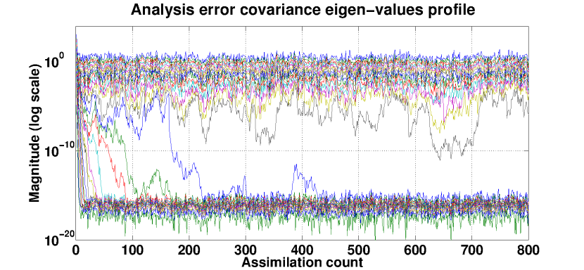
Fig. 1: Profile of the eigen-values of $\Delta_{n}$. Counting establishes that the bottom $16$ eigen-values converge to zero.

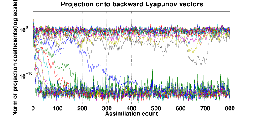
Fig. 2: Norm of the projection
coefficients $\|\Delta_{n}{\mathbf{u}}_{j,n}\|$ for varying observation time $n$.

4 Autonomous linear dynamical systems

4.1 Null space characterization for autonomous systems

The noiseless, linear autonomous system can be defined from equation (2), with the additional assumptions that $A_{n}\equiv A$, $H_{n}\equiv H$, $Q_{n}\equiv Q$, are fixed matrices for all $n$ — therefore the results about the asymptotic rank deficiency property of the error covariance matrices in Section 3 also apply to autonomous systems. However, a stronger statement can be made for time invariant systems because the backwards Lyapunov vectors will not vary in time. In fact, the result in this section is even valid for the case when only the dynamical system is autonomous ($A_{n}\equiv A$) but the observation process is time dependent ($H_{n}$ and $Q_{n}$ depend on $n$).

Akin to the non-autonomous case we define

$$E^{b}_{n}\equiv\left[A^{n}(A^{n})^{\ast}\right]^{\frac{1}{2n}},\quad E^{f}_{n}\equiv\left[(A^{n})^{\ast}A^{n}\right]^{\frac{1}{2n}}$$ (39)

and the similarity with equation (12) can readily be seen by setting $B_{m:m+n}=A^{n},\forall m$ in equation (9) (hence the omission of the time index $m$). As before, the existence of the limits

$$E^{b}\equiv\lim\limits_{n\rightarrow\infty}E^{b}_{n}\,,\quad E^{f}\equiv\lim\limits_{n\rightarrow\infty}E^{f}_{n}$$ (40)

is guaranteed by Oseledets theorem [10]. The eigen-vectors of $E^{b}$ and $E^{f}$ are called the backward and forward Lyapunov vectors, represented here as the columns vectors of $L^{b}$ and $L^{f}$ ordered left to right from the most unstable direction—corresponding to the largest Lyapunov exponent—to the most stable direction—corresponding to the smallest Lyapunov exponent. Specifically, the Lyapunov vectors are defined globally and have no dependence on the time in the linear, autonomous case. Without the time dependence on the backwards stable Lyapunov vectors, we obtain a stronger statement about the asymptotic null space of the covariance matrices.

Definition 11.

Let $L^{bs}\equiv L^{bs}_{n}=\left[{\mathbf{l}}^{b}_{d_{0}+1},\cdots,{\mathbf{l}}^{b}_{d}\right]$. Note that Theorem 19 proved in Appendix B states tells us that the span of the columns of $L^{bs}$ is equal to ${\mathcal{E}}^{1}(A^{T})$

Corollary 12.

Consider the uniformly completely observable, perfect-model, linear, autonomous system defined from equation (2) where $A_{n}\equiv A$, but $H_{n}$ and $Q_{n}$ may depend on $n$ and the initial state ${\mathbf{x}}_{0}$ has a Gaussian law with covariance $\Delta_{0}$. Then the restriction of the analysis and forecast error covariances onto ${\mathcal{E}}^{1}(A^{T})$ tend to zero as $n\rightarrow\infty$. That is

$$\lim_{n\rightarrow\infty}\|\Delta_{n}L^{bs}\left(L^{bs}\right)^{T}\|=0$$ (41)

$$\lim_{n\rightarrow\infty}\|\Sigma_{n}L^{bs}\left(L^{bs}\right)^{T}\|=0$$ (42)

Proof.

Combining Theorem 9 with Theorem 19 this is a straightforward consequence. ∎

In all our numerical simulations with arbitrary (and completely observable) choices of $A$, $H$ and $Q$ we have additionally observed convergence of $\Delta_{n}$ and $\Sigma_{n}$ to a fixed $\Delta$ and $\Sigma$ respectively and seen their null spaces contain ${\mathcal{E}}^{1}\left(A^{T}\right)$ as stated by Corollary 12 (refer Section 4.2). Considering the recent work of Ni et al. [14], this strongly suggests that the classical result of the stable Riccati equation for completely observable and controllable, discrete autonomous systems [9] has an analogue in the case of completely observable, perfect model systems.

4.2 Numerical results for linear autonomous system

We choose a non-singular matrix $A\in\mathbb{R}^{30\times 30}$ ($d=30$) consisting of random entries and set $d_{0}=12$ of its eigen-values to be greater or equal to one in absolute magnitude. We ran the Kalman filtering system long enough and observed that the analysis error covariance do converge to a fixed $\Delta$ and then projected $\Delta$ onto the generalized eigen-space of $A^{T}$. Figure 4 plots the absolute magnitude of eigen-values of $A$ sorted in descending order $\left(\mid\lambda_{1}(A)\mid\geq\cdots\geq\mid\lambda_{d}(A)\mid\right)$ in blue color and shows the Lyapunov exponents for this system in red shade where we note that the number of non-negative Lyapunov exponents is exactly $12$ tantamount to the number of eigen-values of $A$ greater than or equal to one in magnitude. Additionally, it can be verified that the Lyapunov exponents are just the logarithm (to the base $e$) of the absolute magnitude eigen-values of $A$. Recalling the definition of the Lyapunov exponents from equation (15), this equality also lends credence to our Theorem 15. The plot in Figure 4 displays $\|\Delta\left({\mathbf{v}}_{j}\left(A^{T}\right)\right)\|;j\in\{1,2,\cdots,d\}$ where ${\mathbf{v}}_{j}\left(A^{T}\right)$ is the generalized eigen-vector of $\lambda_{j}(A)$. Observe that when $j>12$, the norm of the projected coefficients is zero rendering a visual confirmation to Corollary 12.

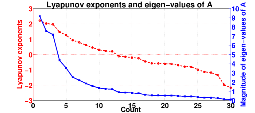
Fig. 3: Lyapunov exponents in blue and the magnitude of the eigen-values of $A$ in red.

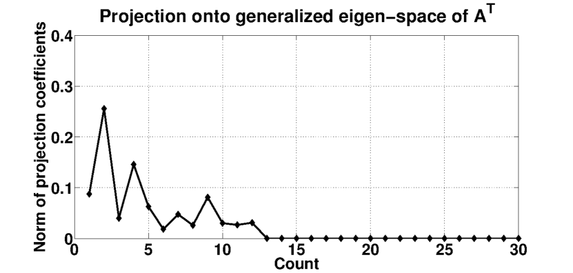
Fig. 4: Norm of the projection coefficients onto the generalized eigen-space of $A^{T}$.

5 Discussion

We have shown that under sequential Kalman filtering, the error covariance for a linear, perfect-model, conditionally Gaussian systems asymptotically collapses to the subspaces spanned by the backwards unstable Lyapunov vectors. This has been known to practitioners in the forecasting community [1], but had yet to be stated in precise mathematical terms. In particular, this foundational work validates the underlying assumptions and methodology of AUS.

At the same time, these results open many new questions for ongoing research related to AUS algorithms. For instance, the present results do not formally show the equivalence of a fully reduced-rank algorithm such as EKF-AUS applied in such a setting. The conditions that imply the convergence of the covariance matrices, given arbitrary low rank symmetric matrices chosen as initial conditions have yet to be established. Recent work strongly suggests that filter stability for discrete, perfect model systems can be demonstrated under sufficient observability hypotheses alone [14]. Determining the necessary hypotheses for stability of the discrete Kalman filter with low rank initializations of the prior covariance matrix in perfect model systems will be the subject of the sequel to our work.

Additionally there are conceptual issues to be resolved in bridging the results for linear systems to non-linear settings; the former having the advantage of Lyapunov vectors being defined globally in space, whereas the formulation must change in a non-linear setting, respecting the dependence on the underlying path. Both of these directions of inquiry open rich areas for mathematical research and future algorithm design.

While the ultimate goal of DA is a precise estimate of state for chaotic dynamics, it is critical to understand the uncertainty of the prediction. An exact calculation of the posterior distribution of states for a high dimensional, complex system is computationally intractable; as computational resources increase, so will model complexity and thus computational efficiency alone will not resolve this issue. This work provides an idealized, but general framework for future investigations into low dimensional approximations for uncertainty calculation. We hope that a precise mathematical framework for understanding the nature of uncertainty for linear systems will lead to innovative research to surmount these challenges.

Appendix A Eigen-values, singular-values and Lyapunov exponents of linear autonomous systems

The results established in this Appendix and Appendix B should be treated as an independent body of work elucidating the relationship between various concepts in linear, autonomous systems and not restricted to the domain of DA and filtering theory. While these relationships are known and can be retrieved from multiple sources in the literature, we have explicitly proved them here for completeness. Readers familiar with these mathematical connections may choose to skip through these sections without any loss of continuity.

Based on the definition of the matrix $E^{f}_{n}$ in equation (39) we find $\lambda_{j}(E^{f}_{n})=\left[\sigma_{j}(A^{n})\right]^{\frac{1}{n}}$. As $E^{f}_{n}\rightarrow E^{f}$ we also have

$$\begin{matrix}\lim\limits_{n\rightarrow\infty}\lambda_{j}(E^{f}_{n})=\lim\limits_{n\rightarrow\infty}\left[\sigma_{j}(A^{n})\right]^{\frac{1}{n}}=\lambda_{j}(E^{f})&&j\in\{1,2,\cdots,d\}\end{matrix}$$ (43)

where the eigen-values $\lambda_{j}$ and singular-values $\sigma_{j}$ are ordered descending in norm. Dropping the label for brevity let $J=V_{A}^{-1}AV_{A}$ (instead of $J(A)$) be the Jordan canonical form of $A$. It is straightforward to see that $A^{n}=V_{A}J^{n}V_{A}^{-1}$ for any integer $n$. The following inequality stated in Theorem 9 of [12] is quite useful. For any two square matrices $Z_{1}$ and $Z_{2}$ we have

$$\begin{matrix}\sigma_{j}(Z_{1})\sigma_{d}(Z_{2})&\leq&\sigma_{j}(Z_{1}Z_{2})&\leq&\sigma_{j}(Z_{1})\sigma_{1}(Z_{2})\end{matrix}$$ (44)

Since the singular-values of both the matrix and its transpose are the same, it follows that

$$\begin{matrix}\sigma_{d}(Z_{1})\sigma_{j}(Z_{2})&\leq&\sigma_{j}(Z_{1}Z_{2})&\leq&\sigma_{1}(Z_{1})\sigma_{j}(Z_{2}).\end{matrix}$$ (45)

Lemma 13.

For any square matrix $Z=V_{Z}J(Z)V_{Z}^{-1}$

$$\lim\limits_{n\rightarrow\infty}\left[\sigma_{j}(Z^{n})\right]^{\frac{1}{n}}=\lim\limits_{n\rightarrow\infty}\left[\sigma_{j}(J(Z)^{n})\right]^{\frac{1}{n}}$$

Proof.

Inequalities (44) and (45) leads to

$$\sigma_{d}\left(V_{Z}\right)\sigma_{d}\left(V_{Z}^{-1}\right)\sigma_{j}(J(Z)^{n})\leq\sigma_{j}(Z^{n})\leq\sigma_{1}\left(V_{Z}\right)\sigma_{1}\left(V_{Z}^{-1}\right)\sigma_{j}(J(Z)^{n}).$$

Raising each term to the power $1/n$ and letting $n\rightarrow\infty$ proves the result. ∎

Corollary 14.

For any matrix $A$ let $E^{f}$ be defined as in equation (40) and $J$ be the Jordan canonical form of $A$. Then $\lambda_{j}(E^{f})=\lim\limits_{n\rightarrow\infty}\left[\sigma_{j}(J^{n})\right]^{\frac{1}{n}},j\in\{1,2,\cdots,d\}.$

Proof.

The results follows immediately when we employ Lemma 13 setting $Z=A$ in conjunction with equation (43). ∎

The theorem below establishes the relation between the eigen-values of the time invariant propagator $A$ and the limit matrix $E^{f}$.

Theorem 15.

For any matrix $A$ let the matrix $E^{f}$ be defined as in equation (40). Then the eigen-values of $E^{f}$ equal the absolute magnitude eigen-values of $A$, i.e, $\lambda_{j}(E^{f})=\left|\lambda_{j}(A)\right|,j\in\{1,2,\ldots,d\}$.

Proof.

We consider two different cases.

case 1: $A$ is diagonalizable. When $J$ is diagonal then $\sigma_{j}(J)=\left|\lambda_{j}(J)\right|=\left|\lambda_{j}(A)\right|$. Recalling that $\lambda_{j}(J^{n})=\left[\lambda_{j}(J)\right]^{n},\forall n$, we get $\left[\sigma_{j}(J^{n})\right]^{\frac{1}{n}}=\left|\lambda_{j}(A)\right|$ and the result follows from Corollary 14.

case 2: $A$ is not diagonalizable. Let $J_{\lambda}(A)$ denote the Jordan-block of size $k\times k$ corresponding to an eigen-value $\lambda$ of $A$ of the form

$$J_{\lambda}(A)\equiv\begin{pmatrix}\lambda&1&0&\cdots&0\\ 0&\lambda&1&\cdots&0\\ \vdots&\vdots&\vdots&\vdots&\vdots\\ 0&0&0&\lambda&1\\ 0&0&0&0&\lambda\end{pmatrix}.$$ (46)

The following lemma is useful in proving Theorem 15.

Lemma 16.

For any matrix $A$ let $J_{\lambda}(A)$ be a Jordan block corresponding to eigen-value $\lambda$ of $A$ as defined in equation (46). Then the singular-values of $J_{\lambda}(A)$ respect the following equality, namely

$$\begin{matrix}\lim\limits_{n\rightarrow\infty}\left[\sigma_{j}\left(J_{\lambda}^{n}\right)\right]^{\frac{1}{n}}=|\lambda|&&j\in\{1,2,\cdots,k\},\end{matrix}$$ (47)

i.e, the limiting singular-values are the absolute magnitude of their respective eigen-values.

Proof.

Following the standard proof technique for equality results we individually show that

$$\begin{matrix}\lim\limits_{n\rightarrow\infty}\left[\sigma_{j}\left(J_{\lambda}^{n}\right)\right]^{\frac{1}{n}}\leq|\lambda|&&j\in\{1,2,\cdots,k\}\end{matrix}$$ (48)

and

$$\begin{matrix}\lim\limits_{n\rightarrow\infty}\left[\sigma_{j}\left(J_{\lambda}^{n}\right)\right]^{\frac{1}{n}}\geq|\lambda|&&j\in\{1,2,\cdots,k\}.\end{matrix}$$ (49)

Let the Nilponent matrix $N\equiv J_{\lambda}-\lambda I$ with $N^{k}=\mathbf{0}$. When $n\geq k-1$ we get

$$\begin{matrix}J_{\lambda}^{n}&=&\left(\lambda I+N\right)^{n}&=&\sum\limits_{r=0}^{k-1}\binom{n}{r}\lambda^{n-r}N^{r}.\end{matrix}$$

Further, the highest singular-value $\sigma_{1}(N^{r})=1$ for $r\in\{0,1,\cdots,k-1\}$. If $\lambda=0$ then $J_{\lambda}^{n}=\mathbf{0}$ when $n\geq k-1$ and the result is trivially true. Suppose $\lambda\not=0$ define $\delta\equiv\frac{1}{\lambda}$. Using the identity that for any two matrices $Z_{1}$ and $Z_{2}$, $\sigma_{1}(Z_{1}+Z_{2})\leq\sigma_{1}(Z_{1})+\sigma_{1}(Z_{2})$ as stated in Theorem 6 of [12], we have

$$\sigma_{1}\left(J_{\lambda}^{n}\right)\leq|\lambda|^{n}\left[\sum_{r=0}^{k-1}\binom{n}{r}|\delta|^{r}\right].$$ (50)

Let $|\delta|=\epsilon\xi$ for any $0<\epsilon\leq|\delta|$. Then

$$\sigma_{1}\left(J_{\lambda}^{n}\right) \leq|\lambda|^{n}\xi^{k}\left[\sum_{r=0}^{k-1}\binom{n}{r}\epsilon^{r}\right]$$

$$\leq|\lambda|^{n}\xi^{k}\left[\sum_{r=0}^{n}\binom{n}{r}\epsilon^{r}\right]=|\lambda|^{n}\xi^{k}(1+\epsilon)^{n}$$

Raising to the power $1/n$ and taking the limit we get

$$\lim_{n\rightarrow\infty}\left[\sigma_{1}\left(J_{\lambda}^{n}\right)\right]^{\frac{1}{n}}\leq|\lambda|(1+\epsilon).$$

The above inequality is also true for the rest of the singular-values as $\sigma_{1}(.)$ is the largest. Since $\epsilon$ is arbitrary the first inequality (48) follows. If $\lambda=0$ we get the desired, stronger equality result in equation (47) as the singular-values by definition are non-negative. It suffices to focus on the case $\lambda\not=0$ where $J_{\lambda}$ is invertible.

To establish the reverse inequality (49), let $T_{\lambda}$ be the Jordan canonical form of $J_{\lambda}^{-1}$ given by

$$T_{\lambda}\equiv\begin{pmatrix}\frac{1}{\lambda}&1&0&\cdots&0\\ 0&\frac{1}{\lambda}&1&\cdots&0\\ \vdots&\vdots&\vdots&\vdots&\vdots\\ 0&0&0&\frac{1}{\lambda}&1\\ 0&0&0&0&\frac{1}{\lambda}\end{pmatrix}.$$

Lemma 13 entails that

$$\lim\limits_{n\rightarrow\infty}\left[\sigma_{j}\left(\left(J_{\lambda}^{-1}\right)^{n}\right)\right]^{\frac{1}{n}}=\lim\limits_{n\rightarrow\infty}\left[\sigma_{j}(T_{\lambda}^{n})\right]^{\frac{1}{n}}.$$

Applying the inequality (48) on $T_{\lambda}$ gives us

$$\begin{matrix}\lim\limits_{n\rightarrow\infty}\left[\sigma_{j}\left(T_{\lambda}^{n}\right)\right]^{\frac{1}{n}}\leq\frac{1}{|\lambda|}&&j\in\{1,2,\cdots,k\}.\end{matrix}$$

In particular,

$$\lim_{n\rightarrow\infty}\left[\sigma_{1}\left(\left(J_{\lambda}^{-1}\right)^{n}\right)\right]^{\frac{1}{n}}=\lim\limits_{n\rightarrow\infty}\frac{1}{\left[\sigma_{k}\left(J_{\lambda}^{n}\right)\right]^{\frac{1}{n}}}\leq\frac{1}{|\lambda|}$$

where the equality stems from the fact that for any invertible matrix $Z$ of size $k\times k$

$$\sigma_{j}\left(Z^{-1}\right)=\frac{1}{\sigma_{k-j+1}\left(Z\right)}.$$

We then get

$$\lim\limits_{n\rightarrow\infty}\left[\sigma_{k}(J_{\lambda}^{n})\right]^{\frac{1}{n}}\geq|\lambda|.$$ (51)

Since $\sigma_{k}(.)$ is the smallest singular-value the inequality (51) is also valid for the rest. ∎

Now to prove Theorem 15 note that for any $n$

$$J^{n}=\begin{pmatrix}J_{\lambda_{1}}^{n}&0&\cdots&0\\ 0&J_{\lambda_{2}}^{n}&\cdots&0\\ \vdots&\vdots&\ddots&\vdots\\ 0&0&\cdots&J_{\lambda_{l}}^{n}\end{pmatrix}$$

is a block diagonal matrix and the eigen-(singular) values of $J^{n}$ equals the disjoint union of eigen-(singular) values of individual Jordan blocks $J_{\lambda_{1}}^{n},\cdots,J_{\lambda_{l}}^{n}$. In accordance with Corollary 14 and Lemma 16 we find $\forall j\in\{1,2,\ldots,d\}$,

$$\lambda_{j}(E^{f})=\lim\limits_{n\rightarrow\infty}\left[\sigma_{j}(J^{n})\right]^{\frac{1}{n}}=\left|\lambda_{j}(J)\right|=\left|\lambda_{j}(A)\right|.$$

∎

Appendix B Eigen-spaces and Lyapunov vectors of linear autonomous systems

By a suitable coordinate transformation, namely ${\mathbf{z}}_{n}=V_{A}^{-1}{\mathbf{x}}_{n}$, studying the dynamics ${\mathbf{x}}_{n+1}=A{\mathbf{x}}_{n}$ is tantamount to investigating ${\mathbf{z}}_{n+1}=J{\mathbf{z}}_{n}$ where $J=V_{A}^{-1}AV_{A}$ is the Jordan canonical form of $A$. Indeed,

$${\mathbf{z}}_{n+1} =J{\mathbf{z}}_{n}=V_{A}^{-1}AV_{A}V_{A}^{-1}{\mathbf{x}}_{n}=V_{A}^{-1}{\mathbf{x}}_{n+1}.$$

Corresponding to the definitions of the matrices $E^{f}_{n}$ and $E^{f}$ in equations (39)-(40), let $G_{n}\equiv\left[(J^{n})^{\ast}J^{n}\right]^{\frac{1}{2n}}$ and let $G\equiv\lim\limits_{n\rightarrow\infty}G_{n}$.

We consider the two systems in the different $d$ dimensional spaces ${\mathbb{R}_{A}^{d}}$ and ${\mathbb{C}_{J}^{d}}$ where the underlying propagators are $A$ and $J$ respectively. Note that as the matrix $V_{A}$ might be complex (though $A$ is real) the dynamics for the propagator $J$ is examined in a complex state space.

Lemma 17.

If the scalar product in ${\mathbb{C}_{J}^{d}}$ is the canonical one namely, $\langle{\mathbf{u}},{\mathbf{v}}\rangle_{J}={\mathbf{u}}^{\dagger}{\mathbf{v}}$, then $V_{G}=I_{d}$ where $I_{d}$ is the $d\times d$ identity matrix.

Proof.

We find it convenient to handle the following scenarios separately.

case 1: $A$ is diagonalizable. $J$ is diagonal and so is $J^{n}$. In the canonical inner product setting the entries of the diagonal $G_{n}$ are the absolute magnitude entries of $J$. It follows that $G$ is diagonal and $V_{G}=V_{J}=I_{d}$.

case 2: $A$ is not diagonalizable. As before, consider the Jordan block $J_{\lambda}$ given in equation (46) of size $k\times k$ corresponding to the eigen-value $\lambda$. Define $G_{\lambda}\equiv\lim\limits_{n\rightarrow\infty}\left[(J_{\lambda}^{n})^{\ast}J_{\lambda}^{n}\right]^{\frac{1}{2n}}$. Since $G_{\lambda}$ is symmetric it is diagonalizable and by Theorem 15 we have $\lambda_{j}\left(G_{\lambda}\right)=|\lambda|,\forall j\in\{1,2,\cdots,k\}$. As all the eigen-values of $G_{\lambda}$ are equal, it is a scalar matrix and therefore we can choose $V_{G_{\lambda}}=I_{k}$. Since

$$G=\begin{pmatrix}G_{\lambda_{1}}&0&\cdots&0\\ 0&G_{\lambda_{2}}&\cdots&0\\ \vdots&\vdots&\ddots&\vdots\\ 0&0&\cdots&G_{\lambda_{l}}\end{pmatrix}$$

the result follows. ∎

Lemma 18.

Under the definition of the scalar products $\langle{\mathbf{u}},{\mathbf{v}}\rangle_{J}={\mathbf{u}}^{{\dagger}}V_{A}^{\dagger}V_{A}{\mathbf{v}}$ in ${\mathbb{C}_{J}^{d}}$ and $\langle{\mathbf{u}},{\mathbf{v}}\rangle_{A}={\mathbf{u}}^{T}{\mathbf{v}}$ in ${\mathbb{R}_{A}^{d}}$, $V_{G}=V_{A}^{-1}V_{E^{f}}$.

Proof.

For the aforesaid considerations of the scalar products in ${\mathbb{C}_{J}^{d}}$ and ${\mathbb{R}_{A}^{d}}$, $J^{\ast}=\left(V_{A}^{{\dagger}}V_{A}\right)^{-1}J^{\dagger}V_{A}^{{\dagger}}V_{A}$ and $A^{\ast}=A^{T}$ respectively. Recalling that $J=V_{A}^{-1}AV_{A}$ we have

$$(J^{n})^{\ast} =\left(V_{A}^{{\dagger}}V_{A}\right)^{-1}V_{A}^{\dagger}\left(A^{n}\right)^{T}\left(V_{A}^{-1}\right)^{\dagger}V_{A}^{{\dagger}}V_{A}=V_{A}^{-1}\left(A^{n}\right)^{T}V_{A}$$

$$\Rightarrow G_{n} =\left[V_{A}^{-1}\left(A^{n}\right)^{T}V_{A}V_{A}^{-1}A^{n}V_{A}\right]^{\frac{1}{2n}}=\left[V_{A}^{-1}\left(A^{n}\right)^{T}A^{n}V_{A}\right]^{\frac{1}{2n}}.$$

As $\left(E^{f}_{n}\right)^{2n}=\left(A^{n}\right)^{T}A^{n}$ is symmetric, it is diagonalizable by an orthonormal matrix $V_{E^{f}_{n}}$ and carries a representation $\left(E^{f}_{n}\right)^{2n}=V_{E^{f}_{n}}(\Lambda_{E^{f}_{n}})^{2n}V_{E^{f}_{n}}^{T}$. We find $\Lambda_{G_{n}}=\Lambda_{E_{n}}$ and $V_{G_{n}}=V_{A}^{-1}V_{E_{n}},\forall n$ and the result follows by letting $n\rightarrow\infty$. ∎

Recall the real span ${\mathcal{T}}_{\mathbf{w}}$ from Definition 1 bearing in mind the complex generalized eigenvectors of any matrix $Z$ always occur in conjugate pairs $\{{\mathbf{w}},\overline{{\mathbf{w}}}\}$ with ${\mathcal{T}}_{{\mathbf{w}}}={\mathcal{T}}_{\overline{{\mathbf{w}}}}$. We have the following theorem, namely

Theorem 19 (Eigenspace equality).

For any matrix $A$ let the matrix $E^{f}$ be defined as in equation (40). Then for any $\alpha\geq 0$ the corresponding $\alpha$-eigenspaces of $E^{f}$ and $A$ are the same, i.e, ${\mathcal{E}^{\alpha}}\left(E^{f}\right)={\mathcal{E}^{\alpha}}(A)$. Equivalently, ${\mathcal{E}^{\alpha}}\left(E^{b}\right)={\mathcal{E}^{\alpha}}\left(A^{T}\right)$.

Proof.

By Theorem 15 we have $\lambda_{j}(G)=|\lambda_{j}(J)|=|\lambda_{j}(A)|=\lambda_{j}(E^{f})$. Recall that the eigen-values are ordered with $\lambda_{1}(G)$ and $\lambda_{d}(G)$ being the largest and the smallest respectively. Oseledets theorem states that there exits a sequence of embedded subspaces

$$0\subset{\mathcal{F}}_{d}\subset{\mathcal{F}}_{d-1}\subset\cdots\subset{\mathcal{F}}_{1}={\mathbb{C}_{J}^{d}}$$

such that on the complement ${\mathcal{F}}_{j}\backslash{\mathcal{F}}_{j+1}$ of ${\mathcal{F}}_{j+1}$ in ${\mathcal{F}}_{j}$ the growth rate is at most $\lambda_{j}(G)$ [15]. The subspaces ${\mathcal{F}}_{j}$ can be obtained as the direct sum of the eigenvectors ${\mathbf{v}}_{j}(G)$ as

$${\mathcal{F}}_{j}={\mathbf{v}}_{d}(G)\oplus{\mathbf{v}}_{d-1}(G)\oplus\cdots\oplus{\mathbf{v}}_{j}(G)$$

where ${\mathbf{v}}_{j}(G)$ is the eigenvector of $G$ corresponding to $\lambda_{j}(G)$. Further, though the eigenvectors of $G$ depend on the underlying scalar product in ${\mathbb{C}_{J}^{d}}$, the embedded subspaces ${\mathcal{F}}_{j}$ and the eigen-values $\lambda_{j}(G)$ are independent of it [10].

Corresponding to the two inner-product definitions in ${\mathbb{C}_{J}^{d}}$, specifically $\langle{\mathbf{u}},{\mathbf{v}}\rangle_{J}={\mathbf{u}}^{\dagger}{\mathbf{v}}$ and $\langle{\mathbf{u}},{\mathbf{v}}\rangle_{J}={\mathbf{u}}^{\dagger}V_{A}^{\dagger}V_{A}{\mathbf{v}}$ we denote the respective eigenvectors with the superscript symbols $1$ and $2$. By Lemma 17 we have $V_{G}^{1}=I_{d}=V_{A}^{-1}V_{A}$ and Lemma 18 declares that $V_{G}^{2}=V_{A}^{-1}V_{E^{f}}$ where $V_{E^{f}}$ is computed using the canonical inner product in ${\mathbb{R}_{A}^{d}}$. For the given $\alpha$ let $q=\operatorname*{\arg\!\min}_{j}\lambda_{j}(G)\leq\alpha$. The invariance of the embedded subspace ${\mathcal{F}}_{q}$ to the underlying scalar product signifies that the real span of the vectors $\{V_{A}{\mathbf{v}}_{d}^{1}(G),\cdots,V_{A}{\mathbf{v}}_{q}^{1}(G)\}$ equal the real span of the vectors $\{V_{A}{\mathbf{v}}_{d}^{2}(G),\cdots,V_{A}{\mathbf{v}}_{q}^{2}(G)\}$. As $\forall j\in\{1,2,\cdots,d\},V_{A}{\mathbf{v}}_{j}^{1}(G)={\mathbf{v}}_{j}(A)$ and $V_{A}{\mathbf{v}}_{j}^{2}(G)={\mathbf{v}}_{j}(E^{f})$, the result follows. ∎

References

- [1] S. Bonnabel and R. Sepulchre, The geometry of low-rank Kalman filters, in Matrix Inf. Geom., F. Nielsen and R. Bhatia, eds., Springer Berlin Heidelberg, 2013, pp. 53–68.
- [2] P. Bougerol, Kalman filtering with random coefficients and contractions, SIAM J. Control Optim., 31 (1993), pp. 942–959.
- [3] A. Carrassi, A. Trevisan, L. Descamps, O. Talagrand, and F. Uboldi, Controlling instabilities along a 3DVar analysis cycle by assimilating in the unstable subspace: a comparison with the EnKF, Nonlinear Process. Geophys., 15 (2008), pp. 503–521.
- [4] S. E. Cohn, An introduction to estimation theory, J. Meteor. Soc. Japan, 75 (1997), pp. 257–288.
- [5] G. Evensen, Data assimilation: The ensemble Kalman filter, Springer, New York, 2009.
- [6] M. Ghil and P. Malanotte-Rizzoli, Data assimilation in meteorology and oceanography, Adv. Geophys., 33 (1991), pp. 141–266.
- [7] A. H. Jazwinski, Stochastic processes and filtering theory, Academic Press, New York, 1970.
- [8] R. Kalman, A new approach to linear filtering and prediction problems, Trans. ASME J. Basic Eng., 82 (1960), pp. 35–45.
- [9] P. R. Kumar and P. Varaiya, Stochastic systems: Estimation, identification and adaptive control, Prentice Hall, New Jersey, 1986.
- [10] B. Legras and R. Vautard, A guide to Lyapunov vectors, in Predictability Seminar Proc., T. Palmer, ed., vol. 1 of ECWF Seminar, 1996, pp. 135–146.
- [11] E. N. Lorenz, Deterministic non-periodic flow, J. Atmos. Sci., 20 (1963), pp. 130–141.
- [12] J. K. Merikoshi and R. Kumar, Inequalities for spreads of matrix sums and products, Appl. Math. E-Notes, 4 (2004), pp. 150–159.
- [13] R. N. Miller, M. Ghil, and F. Gauthiez, Advanced data assimilation in strongly nonlinear dynamical systems, J. Atmos. Sci., 51 (1994), pp. 1037–1056.
- [14] Boyi Ni and Qinghua Zhang, Stability of the kalman filter for continuous time output error systems, Systems & Control Letters, 94 (2016), pp. 172 – 180.
- [15] V. I. Oseledets, Multiplicative ergodic theorem: Lyapunov characteristic numbers for dynamical systems, Trans. Moscow Math. Soc., 19 (1968), pp. 197–231.
- [16] L. Palatella, A. Carrassi, and A. Trevisan, Lyapunov vectors and assimilation in the unstable subspace: Theory and applications, J. Phys. A, 46 (2013), p. 254020.
- [17] L. Palatella, A. Trevisan, and S. Rambaldi, Nonlinear stability of traffic models and the use of Lyapunov vectors for estimating the traffic state, Phys. Rev. E, 88 (2013), p. 022901.
- [18] C. Pires, R. Vautard, and O. Talagrand, On extending the limits of variational assimilation in nonlinear chaotic systems, Tellus A, 48 (1996), pp. 96–121.
- [19] D. Sanz-Alonso and A. M. Stuart, Long-time asymptotics of the filtering distribution for partially observed chaotic dynamical systems. \urlhttp://arxiv.org/abs/1411.6510.
- [20] O. Talagrand, Assimilation of observations, an introduction, J. Meteor. Soc. Japan, 75 (1997), pp. 191–209.
- [21] A. Trevisan, M. D’Isidoro, and O. Talagrand, Four-dimensional variational assimilation in the unstable subspace and the optimal subspace dimension, Quart. J. Roy. Meteor. Soc., 2010 (2010), pp. 487–496.
- [22] A. Trevisan and L. Palatella, On the Kalman filter error covariance collapse into the unstable subspace, Nonlinear Process. Geophys., 18 (2011), pp. 243–250.
- [23] A. Trevisan and F. Uboldi, Assimilation of standard and targeted observations within the unstable subspace of the observation-analysis-forecast cycle, J. Atmos. Sci., 61 (2004), pp. 103–113.
- [24] F. Uboldi and A. Trevisan, Detecting unstable structures and controlling error growth by assimilation of standard and adaptive observations in a primitive equation ocean model, Nonlinear Process. Geophys., 16 (2006), pp. 67–81.
- [25] M. P. Wojtowski, Geometry of Kalman filters, J. Geom. and Symmetry in Physics, 9 (2007), pp. 83–95.