Ultra-Fast Shapelets for Time Series Classification

Abstract

Time series shapelets are discriminative subsequences and their similarity to a time series can be used for time series classification. Since the discovery of time series shapelets is costly in terms of time, the applicability on long or multivariate time series is difficult. In this work we propose Ultra-Fast Shapelets that uses a number of random shapelets. It is shown that Ultra-Fast Shapelets yield the same prediction quality as current state-of-the-art shapelet-based time series classifiers that carefully select the shapelets by being by up to three orders of magnitudes. Since this method allows a ultra-fast shapelet discovery, using shapelets for long multivariate time series classification becomes feasible.

A method for using shapelets for multivariate time series is proposed and Ultra-Fast Shapelets is proven to be successful in comparison to state-of-the-art multivariate time series classifiers on 15 multivariate time series datasets from various domains. Finally, time series derivatives that have proven to be useful for other time series classifiers are investigated for the shapelet-based classifiers. It is shown that they have a positive impact and that they are easy to integrate with a simple preprocessing step, without the need of adapting the shapelet discovery algorithm.

1 Introduction

Time series classification is a field of significant interest for researchers because time series occur in various domains such as finance, multimedia, medicine and more. A time series is a sequence of data points that have a temporal relation between each other. For time series classification it is common to identify motifs or local patterns that have discrimination quality towards the target variable. One popular method is to identify shapelets [1]. Shapelets are discriminative subsequences and have the property that the distance between a shapelet and its best matching subsequence of a time series is a good predictor for time series classification. Many methods try to find shapelets and apply Shapelet Transformation [2]. Shapelet Transformation is the data transformation method that is used to convert the raw time series data using the shapelets to a different data representation that contains features that correspond to a specific shapelet and its value is the minimal distance to the time series (see Section 4.2.1). The idea of shapelets was mainly applied for univariate time series classification but also for time series clustering [3] and early classification of multivariate time series [4].

One of the biggest problems of shapelet discovery is that it is very time-consuming. Hence, there are various methods of pruning the candidate space [5], improving the scoring function that defines how good a shapelet is [6, 1] or by parallelization [7]. Nevertheless, discovering shapelets remains a slow procedure and is infeasible for large datasets.

We want to tackle the problem of slow shapelet discovery by introducing an unsupervised method that does not need to compute the prediction accuracy of each single candidate. Instead a pool of unsupervised, sampled shapelets is computed and a model is learned in the end. The idea is to exploit the fact that discriminative motifs are appearing frequently. This improves the shapelet discovery process and still a good accuracy can be achieved. This effect is shown in Figure 1.

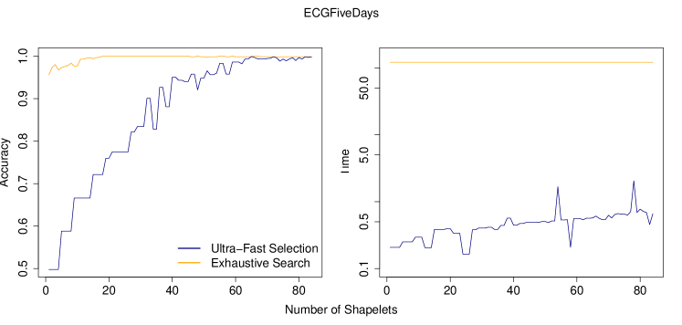
Figure 1: Comparing accuracy and runtime for exhaustively searching the best shapelets or selecting them at random. The same accuracy can be achieved by randomly selecting shapelets but in a hundredth of the time.

The contributions are four-fold:

1. An ultra-fast way of extracting time series subsequences is proposed that allows faster feature extraction than any method that tries to identify discriminative subsequences in a supervised way but is still comparable in terms of classification accuracy.

2. We propose a method which allows time series classification on multivariate time series that concatenates features extracted on different streams. This idea is evaluated on 15 datasets from various domains and compared to state-of-the-art methods for multivariate time series classification.

3. Time series derivatives are considered as additional features for shapelet-based classifiers. Its easy integration with a simple preprocessing step is demonstrated as well as the positive impact on the classification accuracy for shapelet-based classifiers.

4. A comparison between different shapelet-based methods using the original authors’ implementation is conducted. Additionally, the sensitivity for the hyperparameter that defines the number of shapelets that are extracted is analyzed.

The remainder of this paper is organized as follows. In the next section related work is presented and delimited from our contributions. In Section 4, the notation and problem as well as a brief background description is provided. Also, our idea of shapelet discovery is presented and motivated and finally extended to multivariate time series classification. The section ends with a discussion about time series derivatives. Afterwards, in Section 5, it is presented that our idea of shapelet discovery is faster than the state-of-the-art but nevertheless as accurate for univariate time series. Finally, on 15 multivariate time series datasets it is empirically proven that our method provides better predictors for classification. The work is concluded in Section 6.

2 Related Work

The concept of shapelets, discriminative subsequences, was first introduced by Ye et al. [1]. The idea is to consider all subsequences of the training data and assess them regarding a scoring function to estimate how predictive they are with respect to the target. The first proposed scoring function was information gain. Also other measures like F-Stat, Kruskall-Wallis and Mood’s median were considered [2, 8]. It is possible to use the extracted subsequences to transform the data and use an arbitrary classifier [2]. Instead of searching shapelets exhaustively, Grabocka et al. [9] try to learn optimal shapelets with respect to the target and report statistically significant improvements in accuracy compared to other shapelet-based classifiers.

Shapelets have been used in many applications such as medicine [4], gesture [10] and gait recognition [11] and even time series clustering [3].

Since a time series dataset usually contains many shapelet candidates, a brute-force search is very time-consuming and hence many speed-up techniques exist. On the one hand, there are smart implementations using early abandon of distance computation and entropy pruning for the information gain heuristic [1]. On the other hand, ideas to trade time for speed and reuse computations and to prune the search space [6] as well as pruning candidates by searching possibly interesting candidates on the SAX representation [5] or using infrequent shapelets [12] are applied. Gordon et al. [13] learn a decision tree using random subsequences. For each split they consider random subsequences and compute the information gain. If for some time no better subsequence was chosen, the subsequence is used for the split.

In comparison to the related work, discriminative subsequences are not assessed using a scoring function. Instead of that, subsequences are chosen at random and subsequences that provide discriminative features are identified during the learning process of a classifier. This leads to a faster feature extraction process without much impact on the classification accuracy. Our method is also not restricted to a specific classifier.

Shapelets are already considered for the multivariate time series classification by Ghalwash et al. [4]. However, they use multivariate instead of univariate shapelets and use them for early classification. We follow a different idea by using univariate shapelets that are specific for a stream and by considering their interaction among each other using the classifier. Hence, interaction between streams are learned and not assumed.

A very common method for multivariate time series classification is to apply dimensionality reduction like singular value decomposition on the data and then use any classifier on this data. This overcomes the problem of time series with varying lengths [14, 15]. Other methods try to use similiarity-based methods that have proven to be useful for univariate time series classification. For example dynamic time warping was applied on multivariate time series in the context of accelerometer-based gesture recognition [16, 17].

Baydogan et al. [18] use a symbolic representation for multivariate time series. This is similar to SAX [19] but in contrast, the symbols are not fixed but learned in a supervised way using random forests.

3 Baselines

As it is later shown, Ultra-Fast Shapelets (UFS) is comparably accurate as any other shapelet-based classifier but needs less time to extract the shapelets. UFS is compared to three different methods to extract shapelets from univariate data. Additionally, the reader will notice that the number of hyperparameters needed for UFS is, in comparison, very low.

3.1 Exhaustive Search (ES)

The exhaustive search (ES) [2, 6, 1] considers every subsequence in the training data and ranks it using a scoring function $s$. As discussed in Section 4.2, this is equivalent to variable ranking. The scoring function $s$ is usually the information gain but also other quality measures like Kruskal-Wallis, F-statistic and Mood’s median were already considered.

As considering all candidates is infeasible for bigger datasets, the candidates are reduced by considering only subsequences of specific lenghts by choosing a minimum and a maximum length, sometimes a stepsize greater than one. Obviously, as the length of the best subsequence length is unknown, this are very sensitive hyperparameters. A further hyperparamater is the number of shapelets that will be chosen. This is also an important hyperparameter as setting it too low might lead to not considering important features and setting it too high adds to much noise for simple classifiers like Nearest Neighbor.

3.2 Fast Shapelets (FS)

Since exhaustively searching shapelets is very slow, the need for a faster way for extracting shapelets exists. Hence, an approximative method, so called Fast Shapelets (FS) [5], was introduced. The idea is reduce the dimension of the data by estimating the SAX representation [19] and searching on the reduced space for features that are likely to be useful. Hence, mapping back from the reduced space to the original space only few candidates are left. The final features are estimated applying variable ranking. Fast Shapelets is the fastest published method for shapelet discovery we are aware of that yields comparable classification accuracy.

Like in the exhaustive search, there exist the hyperparameters to prune the search space by subsequence length. However, it is also possible to simply take all of them. Three new hyperparameters for the dimensionality reduction are needed, i.e. window length, alphabet size and word length, which might be less sensitive.

3.3 Learning Shapelets (LS)

Recently, a complete new idea was presented. Instead of restricting the pool of possible candidates to those found in the training data and simply searching them, Grabocka et al. [9] propose to consider the shapelets to be parameters that are optimized regarding the loss as well. Hence, shapelets are not found using an approximative measure for being useful for a model but directly optimized for it. This means, it has an advantage because the method does not consider a limited set of candidates but can choose arbitrary shapelets. Disadvantages of this method are that its accuracy highly depends on the initial shapelets and not every classification model can be used. The number of hyperparameters is the same as the exhaustive search but it will be shown that the running time can be slower. In the following sections, this method is called Learning Shapelets (LS).

3.4 Symbolic Representation for Multivariate Timeseries

Symbolic Representation for Multivariate Timeseries (SMTS) [18] is not based on shapelets but has its own way of generating features. The idea is to represent time series as histograms of symbols where a symbol represents a leaf of a decision tree. The raw data is transformed such that for each time point $j$ of time series $T_{i}$ with label $y_{i}$ the transformed data contains an instance $\left(j,t_{i,1,j},\ldots,t_{i,s,j},t_{i,2,j}-t_{i,1,j},\ldots,t_{i,m,j}-t_{i,m-1,j}\right)$ with label $y_{i}$. A random forest is trained on the transformed data and its leafs are considered to be the symbols. The number of occurences of a symbol in the raw data is counted and these symbol histograms are used for the final classification step using random forests.

4 Ultra-Fast Shapelets for Univariate and Multivariate Time Series

Shapelets are often defined as discriminative subsequences and extracted using a supervised quality measure. This process corresponds to a feature subset selection [20] that is computational very expensive as there usually exist many possible shapelet candidates.

In Section 4.2 it will be shown that most shapelet discovery methods are nothing else but feature subset selection algorithms. An alternative way which is faster and is based on feature sampling will be presented in Section 4.3. Subsequently, Section 4.4 introduces a way of generating features from multivariate time series using subsequences. Finally, Section 4.5 shows how to integrate derivatives of time series to the proposed concept of Ultra-Fast Shapelets.

4.1 Notation

A univariate time series $T=\left(t_{1},\ldots,t_{m}\right)$ is a sequence of $m$ data points, $t_{i}\in\mathbb{R}$, where $m$ is called the length of the time series. For notational and illustratic convenience, it is assumed that the length of each time series is the same, although the presented methods can handle time series of varying length.

A multivariate time series $T=\left(t_{1},\ldots,t_{m}\right)$ is a sequence of $m$ vectors $t_{i}=\left(t_{i,1},\ldots,t_{i,s}\right)\in\mathbb{R}^{s}$ with $s$ streams where the time series $T_{j}=\left(t_{1,j},\ldots,t_{m,j}\right)$ is called a stream.

A dataset for univariate or multivariate time series classification is a pair
$\mathcal{T}=\left(\left(T_{1},\ldots,T_{n}\right)^{T},Y\right)$ where $Y=\left(y_{1},\ldots,y_{n}\right)\in\left\{1,\ldots,C\right\}^{n}$ and the class of time series $T_{i}$ is $y_{i}$. The classification task is now to use $\mathcal{T}$ to predict the correct classes for further, unseen time series.

A shapelet for a dataset $\mathcal{T}$ is a time series of length $l\leq m$ which is discriminative with respect to the target regarding to a scoring function $s\ :\ span\left(\mathcal{T}\right)\times\mathbb{R}^{l}\rightarrow\mathbb{R}$, where $s$ is usually the information gain.

4.2 Shapelet Discovery as Feature Subset Selection

In this section the relationship between shapelet discovery and feature subset selection is depicted. This relationship holds only for those methods that choose subsequences as shapelets that occur in the training data which is common in many methods [2, 5, 8, 6, 1]. For a better understanding, Shapelet Transformation is described in Section 4.2.1 and shapelet discovery in Section 4.2.2.

4.2.1 Shapelet Transformation for Univariate Time Series

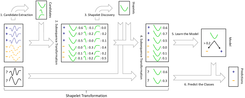
Figure 2: An illustration of the Shapelet Transformation process using a synthetically generated dataset.

The term Shapelet Transformation was introduced by Lines et al. [8]. Shapelet Transformation is a feature extraction process which uses and extracts shapelets which are discriminative subsequences. This idea is used for univariate time series classification latest since Ye et al. [1]. The extracted shapelets are used to express the original time series dataset $\mathcal{T}=\left(\left(T_{1},\ldots,T_{n}\right)^{T},Y\right)$ as a shapelet transformed dataset $\mathcal{D}=\left(X,Y\right)$, $X\in\mathbb{R}^{n\times p}$ which can be done in four steps (see Figure 2):

1. Candidate Extraction: From all time series $T_{1},\ldots,T_{n}$ subsequences $C_{1},\ldots,C_{q}$ are selected to be candidates. There exist different methods to choose the candidates. Typically, all subsequences of a specific length [2, 6, 1] or that fulfill another informed criterion [5] are chosen.

2. Subsequence Transformation: Using the $q$ candidates, the raw data will be transformed. Each candidate $C=\left(c_{1},\ldots,c_{l}\right)$ is a predictor in the new representation and its value for a given time series $T$ is the minimal Euclidean distance on the normalized time series data i.e.

   $$minNormDist\left(C,T\right)=\min_{i=1,\ldots,m-l+1}\left\{\sqrt{\sum_{j=1}^{l}\left(c_{j}-\frac{t_{i+j}-\mu_{T}}{\sigma_{T}}\right)^{2}}\right\}$$ (1)

   where $\mu_{T}$ and $\sigma_{T}$ are the mean and standard deviation of all data points $t_{i}$ of $T$, respectively. Thus, the univariate time series dataset $\mathcal{T}$ can be transformed into a dataset $\mathcal{D}^{\prime}=\left(X^{\prime},Y\right)$, $X^{\prime}\in\mathbb{R}^{n\times q}$ with $x^{\prime}_{i,j}=minNormDist\left(C_{j},T_{i}\right)$. Figure 3 sketches the idea of the minimal distance. The minimal distance between a subsequence and a time series is the Euclidean distance between the subsequence and the best matching subsequence of the time series.

   

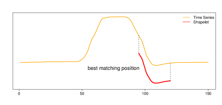
   Figure 3: The minimum distance between a time series and a subsequence: Find the best matching position and compute the Euclidean distance. The time series instance is taken from the GunPoint dataset.

3. Shapelet Discovery: Using a scoring function $s$, all candidates are ranked and the $p$ highest ranked subsequences $S_{1},\ldots,S_{p}$ are selected for further use. All the others are withdrawn.

4. Subsequence Transformation: In the final step of the Shapelet Transformation, the dataset $\mathcal{D}=\left(X,Y\right)$, $X\in\mathbb{R}^{n\times p}$ with $x_{i,j}=minNormDist\left(S_{j},T_{i}\right)$ is computed.

After the completion of the Shapelet Transformation, there are no restrictions whatsoever for a classifier.

4.2.2 Shapelet Discovery is Variable Ranking

The last section has shown how to apply Shapelet Transformation on univariate time series. Now, the relation between shapelet discovery and feature subset selection will be discussed. Therefor, the definition that is used for a shapelet is recited here.

Definition 1

Given is a univariate time series dataset $\mathcal{T}$ and a scoring function $s$ that ranks a subsequence of a time series $T$ according to $\mathcal{T}$. Then, a shapelet $S$ is defined as a subsequence of a time series $T\in\mathcal{T}$ which is among the $p$ highest ranked subsequences regarding to the scoring function $s$.

In the literature this kind of feature subset selection is called variable ranking and is a filter method [20]. Filter methods have the advantage of being computational fast and scalable but have the disadvantages of choosing redundant features and ignore dependencies among features and to the classifier. However, even though variable ranking is one of the fastest feature selection methods, it is still slow for shapelet discovery since the $\mathcal{O}\left(nm^{2}\right)$ features, where $n$ is the number of time series instances and $m$ is the length of a time series, are not given beforehand. First, the minimal distance (Equation 2) needs to be computed before the quality can be assessed.

4.3 Shapelet Discovery as Feature Sampling

Here, a new way of shapelet discovery is proposed. Instead of considering all candidates and applying subsequence transformation and variable ranking (Shapelet Transformation, see Figure 2), the predictors are chosen at random. This idea is sketched in Figure 5. Comparing Figures 2 and Figure 5, one can see that the difference is twofold. For the candidate extraction step a random subset of candidates is chosen and steps 2 and 3 of the Shapelet Transformation, i.e. the feature subset selection, are omitted. From now on, this way of selecting subsequences will be called Ultra-Fast Shapelets.

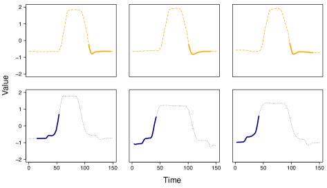
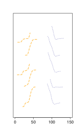
Figure 4: Left: Six random instances from the GunPoint dataset. The task is to decide whether a person is drawing a gun or pointing at something. The dashed, orange plots are showing examples for the pointing class, the dotted, blue plots are showing examples for the gun drawing class. Subsequences that are supposed to be discriminative for a class are highlighted. Right: A selected subset of randomly chosen subsequences of length 35 to 45. The dashed, orange subsequences are chosen from the pointing class, starting before time point 40. The dotted, blue subsequences are chosen from the drawing gun class, starting between time points 80 and 100.

The GunPoint dataset will be used to motivate the idea of Ultra-Fast Shapelets. The GunPoint dataset is an activity recognition dataset where the task is to distinguish whether a human being is lifting his arm to point at something or whether he is drawing a weapon. Example instances of this dataset are shown in Figure 4. This figure also shows the shapelets found using the variable ranking method which are considered to be useful for classification [2]. First, the question is whether similar good subsequences can be found if randomly subsequences of arbitrary length are considered and second, if useless subsequences are a problem. Lets stick to the GunPoint dataset and assume that there are only the two clusters of shapelets shown in Figure 4. Obviously, it is enough to find just one representative for each shapelet cluster since they are redundant and do not give further information. Since they are typical for the data, it is assumed that one out of the two shapelets is found in each time series. The GunPoint dataset contains 50 training instances and hence approximately 50 shapelets. For this dataset $1\%$ of the subsequences are chosen at random. Hence, the probability for finding a representative for both shapelets clusters is quite unlikely. Nevertheless, subsequences within the same interval as one of the shapelets which are a bit longer or shorter are obviously also very good predictors.

In the example, all shapelets are of length 40 but one can assume that subsequences of lengths between 35 and 45 in the same time interval have similar predictive quality. Thus, there are not 50 candidates but 1,230. If one agrees that this holds, the probability of selecting a subsequence which is very close to one of the shapelets discovered by variable ranking is very high. At this point, the reader may have already noticed that there are further discriminative parts that might have not been considered by the variable ranking. Since only the best $p$ features are considered in the variable ranking method and since there are many similar and hence equally high ranked features, the effective number of features in the end can be very small. If $p$ is not chosen high enough, discriminative parts like in the dashed, orange plots around time 50 and in the dotted, blue plots around time 110 (Figure 4) are not considered.

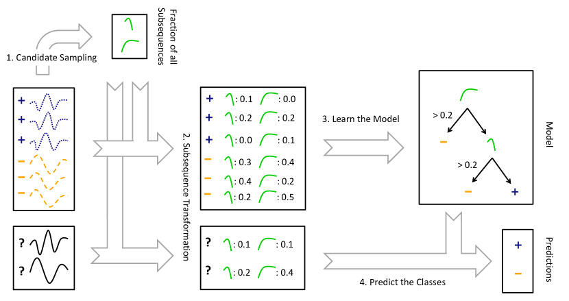
Figure 5: Ultra-Fast Shapelets for time series classification.

Finally, it is more likely that Ultra-Fast Shapelets finds interacting features than variable ranking. Lets think about a dataset with two classes (Figure 6). The one class has either only noise or at least one $\vee$-shaped and one $\wedge$-shaped subsequence which are interrupted by arbitrary long subsequences of noise. The other class either has only subsequences of type $\vee$ divided by subsequences of noise and none of type $\wedge$ or vice versa. If features are extracted by variable ranking, the subsequences $\vee$ and $\wedge$ will have a bad score since the accuracy of each of them alone is about $50\%$ which is as good as random. Therefor, they will not be selected and no good classifier can be trained. On the other hand, Ultra-Fast Shapelets will choose some of them as discussed before and a perfect classifier can be trained.

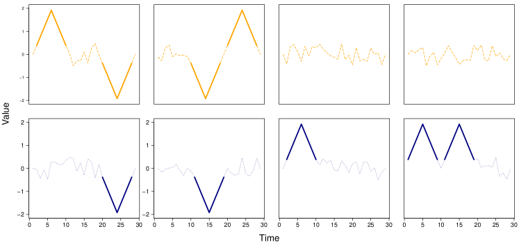
Figure 6: A synthetic dataset where the combination of two subsequences is needed to predict the correct class. The important subsequences can be at any point and arbitrary often.

Concluding, time series contain many duplicates of subsequences where some of them are useful and some are not. This motivates the idea of randomly selecting subsequences. A well regularized classifier can then be used to identify useful subsequences and their interactions.

4.4 Generalized Ultra-Fast Shapelets

This section describes how Ultra-Fast Shapelets can be generalized such that the implementation can be used for univariate and multivariate time series classification. The proposition is to transform multivariate time series using shapelets in a similar way as described for the univariate case before. In the first step, shapelets are chosen at random from each of the $s$ streams such that sets of shapelets $\mathcal{S}_{1},\ldots\mathcal{S}_{s}$ are extracted. Ignoring temporal relations between the streams, the raw data is transformed into a dataset $\mathcal{D}$ such that the features are generated on each stream as in the univariate case and then concatinated. Formally, using the sets $\mathcal{S}_{i}$ of size $\frac{p}{s}$, the dataset $\mathcal{D}=\left(X,Y\right)$, $X\in\mathbb{R}^{n\times p}$ is computed where $x_{i,j}=minDist\left(S_{j-\left(\left\lceil j\frac{s}{p}\right\rceil-1\right)\frac{p}{s}},T_{i,\left\lceil j\frac{s}{p}\right\rceil}\right)$ and $S_{j-\left(\left\lceil j\frac{s}{p}\right\rceil-1\right)\frac{p}{s}}\in\mathcal{S}_{\left\lceil j\frac{s}{p}\right\rceil}$.

Algorithm 1 explains this process in detail. In line 2, the ratio $f$ between the number of features $p$ and the number of all subsequences of arbitrary length is computed. In lines 4-9, subsequences of different length are extracted uniformly at random. After extracting them, the subsequence-transformed dataset is estimated by computing the distance of a subsequence to each time series in lines 12-16. For the distance function in line 16 we have chosen one of the distance functions defined in Equations 1 and 2.

For the experiments on the multivariate datasets, a different distance function between a shapelet and a time series is considered because it provides better results for some datasets: the minimal Euclidean distance between a shapelet and the unnormalized time series

$$minDist\left(S,T\right)=\min_{i=1,\ldots,m-l+1}\left\{\sqrt{\sum_{j=1}^{l}\left(s_{j}-t_{i+j}\right)^{2}}\right\}.$$ (2)

Algorithm 1 Generalized Ultra-Fast Shapelets

0:  Dataset $\mathcal{T}=\left(\left(T_{1},\ldots,T_{n}\right)^{T},Y\right),\ T_{i}\in\mathbb{R}^{m\times s}$, number of features $p$, $c_{1},\ldots,c_{m}$ where $c_{i}$ is the number of all subsequences of length $i$

0:  Subsequence transformed dataset $\left(X,Y\right)$

1:  $\triangleright$ Choose $p$ subsequences at random

2:  $f\leftarrow p\left(\sum_{l=3}^{m}c_{l}\right)^{-1}$

3:  subsequences $\leftarrow\emptyset$

4:  for $l=3$ to $m$ do

5:     for $k=1$ to $s$ do

6:        for $round\left(f\cdot c_{l}\right)$ times do

7:           $i\leftarrow\mathcal{U}\left(1,n\right)$

8:           $j\leftarrow\mathcal{U}\left(1,m-l\right)$

9:           subsequences $\leftarrow$ subsequences $\cup\left\{\left(i,s,j,l\right)\right\}$

10:  

11:  $\triangleright$ Generate the transformed dataset using $\mathcal{T}$ and the subsequences

12:  $X\in\mathbb{R}^{n\times p}$

13:  for $j=1$ to $p$ do

14:     $\left(i^{\prime},s,j^{\prime},l\right)\leftarrow$ subsequences.get(j)

15:     for $i=1$ to $n$ do

16:        $x_{i,j}\leftarrow dist\left(\left(t_{i^{\prime},s,j^{\prime}},\ldots t_{i^{\prime},s,j^{\prime}+l}\right),T_{i,s}\right)$

17:  return  $\left(X,Y\right)$

4.5 Considering Derivatives of Time Series

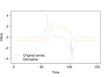
Figure 7: GunPoint time series instance and its time series derivative.

In the next section, Ultra-Fast Shapelets is compared to other state-of-the-art methods for multivariate time series classification. To ensure a fair comparison, the same classification model and the same features shall be used. Since SMTS [18] is not only using the raw time series but also the derivative of it, it is now explained how derivatives can be used for Ultra-Fast Shapelets.

The derivative of a time series $T=\left(t_{1},\ldots,t_{m}\right)$ is defined as $\nabla T=\left(0,t_{2}-t_{1},\ldots,t_{m}-t_{m-1}\right)$. The leading $0$ ensures that the derivative has the same length as its time series. The use of derivatives of time series is straight forward for Ultra-Fast Shapelets. For each stream $T_{i}$ of a time series $T$ a new stream $\nabla T_{i}$ is added which is the derivative of $T_{i}$. The original dataset is now twice that large but no adaption to Algorithm 1 needs to be done. An example for a time series derivative is given in Figure 7.

5 Experiments

In Section 3, the baselines are summarized in order to make this work self-contained. Section 5.1 provides a detailed description of the experimental setup, explaining which hyperparameters are used and how they have been found for every algorithm.

One claim is that sampling of shapelets is in general a scalable way to extract features for time series classification which is also accurate. Therefor, experiments are conducted on 52 univariate datasets from various domains such as speech recognition, activity recognition, medicine, image classification and several more. These datasets are downloaded from [21, 22] and have different properties such as number of training instances, classes and length (see Table 1). In Section 5.2, Ultra-Fast Shapelets (UFS) is compared to various shapelet-based classifiers and its ability to compete is demonstrated. Furthermore, the runtime is compared and it is shown that Ultra-Fast Shapelets is indead faster.

Finally, in Section 5.4, UFS is compared to state-of-the-art classifiers for multivariate time series on 15 datasets from different domains such as speech, gesture, motion, handwriting and sign language recogniton provided by [23]. The number of streams varies between 2 and 62, the number of classes between 2 and 95. In contrast to the univariate datasets, some of the multivariate datasets do not have a fixed length per instance per dataset. A detailed description of the datasets is given in Table 5.

5.1 Experimental Setup

Ultra-Fast Shapelets (UFS) has only a single hyperparameter that is the percentage of considered candidates. Instead of tuning the percentage hyperparameter carefully for all 67 datasets, the highest non-positive power of 10 was chosen such that the number of expected candidates is smaller than 10,000 per stream. For all univariate datasets the normalized distance function defined in Equation 1 was used, for the multivariate datasets this decision was added to the hyperparameter search and then either the distance function defined in Equation 1 or 2 was used.

On the transformed data any classifier may be trained. Random Forest and a linear SVM were chosen because the results for SMTS are reported using a Random Forest and Learning Shapelets is using a linear classifier.

A random forest has three hyperparameters, i.e. the number of trees $J$, the number of sampled features $v$, and the depth $d$ of each tree. A gridsearch was applied on $J\in\left\{20,50,100,500,1000\right\}$, $v\in\left\{\left\lfloor\log\left(p+1\right)\right\rfloor,p\right\}$ and $d\in\left\{5,\ldots,2\log\left(p\right)\right\}$ and evaluated against the out-of-bag error (OOE). The model with smallest OOE was used to classify the test instances. In all experiments the mean over ten repetitions is reported. In case that there was more than one model with the smallest OOE, one was taken at random.

A linear SVM has usually only one hyperparameter, i.e. the regularization term $C$. Another hyperparameter was added that decides whether to use a $L1$ or $L2$-regularized SVM. A gridsearch was applied on $C\in\left\{2^{1},\ldots,2^{10}\right\}$ and both regularization methods. The best combination in a 5-fold cross-validation was used to report the error on test. Again, in all experiments the mean over ten replications is reported.

The results of SMTS, nearest neighbor with dynamic time warping distance without a warping window (NNDTW) and a multivariate extension of TSBF [24] (MTSBF) were taken from Baydogan et al. [18]. Results for the other baselines were redone since the authors only report the accuracy on one run and otherwise the runtime comparison would have not been fair. For the experiments, the implementation provided by the original authors were taken and the hyperparameters were used as proposed by the authors. Because of this and the fact that some datasets are too large, not every baseline is evaluated on every dataset but this shall ensure that the best hyperparameters are chosen. Again, the average over ten replications is reported for every dataset.

5.2 Univariate Datasets

To support the claim that Ultra-Fast Shapelets is comparably to state-of-the-art shapelet-based classifiers with respect to accuracy but faster, experiments are conducted on 52 univariate time series datasets and compared to three different methods of shapelet discovery using various classifiers. Ultra-Fast Shapelets (UFS) using Random Forest (RF) and a linear SVM (SVM) is compared to the exhaustive search of shapelets (ES) using RF and SVM, to Fast Shapelets (FS) and to Learning Shapelets (LS). These four shapelet-based methods are compared based on classification error in Section 5.2.1 and runtime in Section 5.2.2. The experiments show that UFS is as good as state-of-the-art shapelet-based classifiers but scale to large data and therefor can be used for both, univariate and multivariate time series classification, with decent accuracy and runtime. More detailed information about the baselines is given in Section 3.

The datasets are provided by the UCR time series database [22] and by Bagnall et al. [21]. Table 1 contains few statistics about the datasets, further information can be found on the corresponding websites [21, 22].

Table 1: Characteristics of the univariate datasets.

Dataset	Train Instances	Test Instances	Length	Classes	Candidates
50words	450	455	270	50	16,220,700
Adiac	390	391	176	37	5,937,750
Beef	30	30	470	5	3,292,380
CBF	30	900	128	3	240,030
ChlorineConcentration	467	3840	166	3	6,318,510
CinC_ECG_torso	40	1380	1639	4	53,628,120
Coffee	28	28	286	2	1,133,160
Cricket_X	390	390	300	12	17,374,890
Cricket_Y	390	390	300	12	17,374,890
Cricket_Z	390	390	300	12	17,374,890
DiatomSizeReduction	16	306	345	4	943,936
DP_Little	400	645	250	3	12,350,400
DP_Middle	400	645	250	3	12,350,400
DP_Thumb	400	645	250	3	12,350,400
ECG200	100	100	96	2	446,500
ECGFiveDays	23	861	136	2	208,035
FaceAll	560	1690	131	14	4,695,600
FaceFour	24	88	350	4	1,457,424
FacesUCR	200	2050	131	14	1,677,000
FISH	175	175	463	7	18,635,925
Gun_Point	50	150	150	2	551,300
Haptics	155	308	1092	5	92,162,225
InlineSkate	100	550	1882	7	176,814,000
ItalyPowerDemand	67	1029	24	2	16,951
Lighting2	60	61	637	2	12,115,800
Lighting7	70	73	319	7	3,528,210
MALLAT	55	2345	1024	8	28,751,415
MedicalImages	381	760	99	10	1,810,893
MoteStrain	20	1252	84	2	68,060
MP_Little	400	645	250	3	12,350,400
MP_Middle	400	645	250	3	12,350,400
OliveOil	30	30	570	4	4,847,880
OSULeaf	200	242	427	6	18,105,000
Otoliths	64	64	512	2	8,339,520
PP_Little	400	645	250	3	12,350,400
PP_Middle	400	645	250	3	12,350,400
PP_Thumb	400	645	250	3	12,350,400
SonyAIBORobotSurface	20	601	70	2	46,920
SonyAIBORobotSurfaceII	27	953	65	2	54,432
StarLightCurves	1000	8236	1024	3	522,753,000
SwedishLeaf	500	625	128	15	4,000,500
Symbols	25	995	398	6	1,965,150
synthetic_control	300	300	60	6	513,300
Trace	100	100	275	4	3,740,100
TwoLeadECG	23	1139	82	2	74,520
Two_Patterns	1000	4000	128	4	8,001,000
uWaveGestureLibrary_X	896	3582	315	8	44,030,336
uWaveGestureLibrary_Y	896	3582	315	8	44,030,336
uWaveGestureLibrary_Z	896	3582	315	8	44,030,336
wafer	1000	6164	152	2	11,325,000
WordsSynonyms	267	638	270	25	9,624,282
yoga	300	3000	426	2	27,030,000

5.2.1 Classification Accuracy

In this section the results of an empirical comparison on 52 datasets of various domains for different methods of shapelet discovery are presented. Detailed results for each dataset are shown in Table 2.

The different methods can be divided into two groups depending on which kind of classifier they use. The methods that are using a linear SVM (UFS (SVM), ES (SVM), LS) yield better results than those which are using a non-linear, tree-based classifier. The tree-based classifiers are only in 9 datasets better than the SVM which confirms the results by Hills et al. [2]. Overall, FS is the worst classifier which is not surprising because it is an approximation of ES. Comparing UFS with ES by classifier, the performance using a SVM is almost similar. ES has better prediction quality on 10 datasets, UFS on 15. UFS using a random forest shows better performance in 19 datasets and is worse than ES in 7. These results show a strong empirical evidence that simply choosing subsequences at random will not deteriorate the accuracy in comparison to more informative methods like ES or FS.

While LS achieves better accuracy than UFS, it has a higher runtime performance by an average of three orders of magnitude and is the slowest among all investigated methods, as shown in the next section. In that context, the proposed method (UFS) is more scalable than LS for large datasets. In terms of hyperparameters, LS requires three sensitive hyperparameters while our proposed method has only a single insensitive hyperparameter (see Section 5.3). This excludes the classifier-specific hyperparameters for both methods. Finally, one of the reasons that LS is more accurate is that it is not limited in the number of candidates. While ES, FS and UFS can only choose among subsequences that appear in the training set, LS can choose any subsequence.

Table 2: Test error rates averaged over 10 replications for different univariate time series classification methods compared to Ultra-Fast Shapelets on 52 datasets.

Dataset	UFS (SVM)	ES (SVM)	LS	UFS (RF)	ES (RF)	FS	Dataset	UFS (SVM)	UFS (RF)	FS
Adiac	0.276	0.757	0.581	0.281	0.704	0.442	50words	0.184	0.278	0.497
Beef	0.263	0.100	0.193	0.423	0.360	0.483	CBF	0.002	0.014	0.062
ChlorineConcentration	0.262	0.429	0.270	0.357	0.338	0.422	CinC_ECG_torso	0.151	0.199	0.274
Coffee	0.011	0.000	0.000	0.054	0.061	0.075	Cricket_X	0.225	0.294	0.538
DiatomSizeReduction	0.075	0.082	0.058	0.084	0.218	0.131	Cricket_Y	0.234	0.279	0.506
DP_Little	0.293	0.323	0.257	0.315	0.364	0.434	Cricket_Z	0.207	0.248	0.561
DP_Middle	0.288	0.305	0.271	0.288	0.384	0.419	ECG200	0.119	0.187	0.230
DP_Thumb	0.291	0.304	0.264	0.302	0.366	0.420	FaceAll	0.212	0.260	0.366
ECGFiveDays	0.000	0.001	0.000	0.007	0.013	0.004	FacesUCR	0.043	0.090	0.310
FaceFour	0.039	0.023	0.019	0.043	0.226	0.092	FISH	0.035	0.105	0.180
Gun_Point	0.021	0.000	0.006	0.011	0.046	0.068	Haptics	0.509	0.529	0.611
ItalyPowerDemand	0.038	0.065	0.036	0.052	0.072	0.079	InlineSkates	0.618	0.573	0.738
Lighting7	0.222	0.342	0.370	0.264	0.363	0.399	Lighting2	0.213	0.236	0.316
MedicalImages	0.260	0.477	0.336	0.300	0.517	0.392	MALLAT	0.044	0.021	0.058
MoteStrain	0.134	0.119	0.099	0.131	0.148	0.216	OliveOil	0.110	0.123	0.292
MP_Little	0.283	0.293	0.263	0.268	0.336	0.435	OSULeaf	0.158	0.245	0.323
MP_Middle	0.252	0.234	0.241	0.235	0.303	0.395	SonyAIBORobotSurfaceII	0.088	0.121	0.209
Otoliths	0.434	0.359	0.319	0.436	0.364	0.440	StarLightCurves	0.031	0.029	0.054
PP_Little	0.316	0.279	0.297	0.340	0.328	0.451	SwedishLeaf	0.065	0.094	0.225
PP_Middle	0.256	0.287	0.258	0.263	0.329	0.420	Two_Patterns	0.003	0.001	0.079
PP_Thumb	0.304	0.309	0.304	0.342	0.391	0.465	uWaveGestureLibrary_X	0.197	0.191	0.297
SonyAIBORobotSurface	0.122	0.060	0.090	0.109	0.080	0.302	uWaveGestureLibrary_Y	0.291	0.284	0.386
Symbols	0.111	0.167	0.069	0.067	0.176	0.070	uWaveGestureLibrary_Z	0.271	0.238	0.363
synthetic_control	0.006	0.097	0.021	0.009	0.081	0.083	wafer	0.003	0.008	0.002
Trace	0.000	0.000	0.000	0.008	0.000	0.000	WordsSynonyms	0.269	0.376	0.569
TwoLeadECG	0.025	0.000	0.002	0.075	0.064	0.741	yoga	0.129	0.150	0.294

5.2.2 Runtime Analysis

This section shows that Ultra-Fast Shapelets (UFS) is not only as accurate as state-of-the-art methods but also significantly faster which makes it finally feasible to apply shapelets on multivariate time series datasets. Therefor, the four shapelet-based methods are compared empirically and theoretically.

Starting with the empirical runtime analysis, Table 4 provides the measured runtime in seconds averaged over 10 replications for each method on 52 datasets. The subsequence lengths that are considered are those proposed by the authors. This means that only UFS and Fast Shapelets (FS) are considering all candidates while the exhaustive search (ES) and Learning Shapelets (LS) only consider a subset of them. Knowing this, note that this is obviously an advantage for ES and LS. Nevertheless, FS and UFS are significantly faster. UFS is slow compared to the baselines for the small datasets but in general faster which means that it is faster than the fastest shapelet discovery method so far (FS) in 45 out of 52 datasets, in some even by a factor of 100.

The number of all subsequences respectively candidates in a time series dataset with $n$ instances of length $m$ is $c=\mathcal{O}\left(nm^{2}\right)$. Since the exhaustive search compares each possible pair of candidates of equal length, the runtime is $\mathcal{O}\left(n^{2}m^{4}\right)$. FS reduces the number of candidates to a subset $r<c$ which is then compared with all $\mathcal{O}\left(nm^{2}\right)$ candidates of equal length so that FS needs time $\mathcal{O}\left(rnm^{2}\right)$. LS [9] reports a runtime of $\mathcal{O}\left(ipnm^{2}\right)$ where $i$ is the number of iterations used until the algorithm converges and $p$ is the number of shapelets that have to be found. Since the authors propose a very high number of iterations and shapelets for some datasets, a comparably high runtime is observed. Finally, UFS chooses randomly a subset of $p$ candidates, where for the here executed experiments $p<10,000$. Thus, the runtime is $\mathcal{O}\left(pnm^{2}\right)$ and $p<r$ for the larger datasets but $p\approx nm^{2}$ for the very small datasets which explains the high runtime for those. Since the number of candidates $p$ is not optimized but a rule of thumb was used, one can further improve the speed without a loss of accuracy as shown in Section 5.3. Theoretical and empirical results are summarized in Table 3.

Table 3: Summary of theoretical and empirical runtime results. (win/lose)

	UFS	FS	LS	ES
Runtime complexity	$\mathcal{O}\left(pnm^{2}\right)$	$\mathcal{O}\left(rnm^{2}\right)$	$\mathcal{O}\left(ipnm^{2}\right)$	$\mathcal{O}\left(n^{2}m^{4}\right)$
UFS	-	45/7	26/0	23/3
FS	7/45	-	26/0	26/0
LS	0/26	0/26	-	11/15
ES	3/23	0/26	15/11	-

Table 4: Measured time in seconds for learning the model and discovering the shapelets averaged over 10 replications for different shapelet-based univariate time series classification methods compared to Ultra-Fast Shapelets on 52 datasets.

Dataset	UFS	FS	LS	ES	Dataset	UFS	FS
Adiac	45.8	332.6	203847.0	5522.6	50words	23.2	2198.1
Beef	8.3	196.9	25063.5	2148.0	CBF	8.7	10.9
ChlorineConcentration	271.9	760.3	30743.7	13756.5	CinC_ECG_torso	3201.6	4398.9
Coffee	1.6	22.5	372.6	204.7	Cricket_X	25.7	3756.0
DiatomSizeReduction	63.4	15.6	14184.1	94.4	Cricket_Y	26.6	3605.7
DP_Little	17.1	975.1	8384.8	66570.1	Cricket_Z	25.9	4679.2
DP_Middle	17.3	996.1	23875.4	143041.5	ECG200	2.7	16.3
DP_Thumb	17.9	916.3	9107.0	109388.6	FaceAll	58.8	757.5
ECGFiveDays	10.9	3.6	59.2	122.0	FacesUCR	19.1	280.3
FaceFour	5.6	102.9	11078.3	4384.8	FISH	244.4	935.6
Gun_Point	0.7	9.5	1475.3	474.1	Haptics	818.0	12491.0
ItalyPowerDemand	1.8	0.4	20.8	1.5	InlineSkate	637.0	22677.2
Lighting7	10.1	322.8	3902.6	13409.5	Lighting2	11.1	1131.3
MedicalImages	7.4	371.5	6457.7	11084.6	MALLAT	121.7	1736.5
MoteStrain	17.2	3.1	410.5	7.8	OliveOil	16.8	107.2
MP_Little	18.1	996.5	55964.1	75666.3	OSULeaf	26.5	1629.7
MP_Middle	17.0	993.3	6797.5	117056.5	SonyAIBORobotSurfaceII	8.4	1.3
Otoliths	47.5	303.2	9453.2	46546.0	StarLightCurves	8278.9	21473.5
PP_Little	17.3	918.8	27699.3	67944.0	SwedishLeaf	23.5	451.7
PP_Middle	17.0	950.2	35425.6	52285.4	Two_Patterns	147.0	957.2
PP_Thumb	17.5	943.7	67798.2	77402.3	uWaveGestureLibrary_X	344.6	4827.5
SonyAIBORobotSurface	4.9	1.1	115.0	8.5	uWaveGestureLibrary_Y	348.9	4379.6
Symbols	52.0	93.0	1104.3	12511.4	uWaveGestureLibrary_Z	497.0	5215.9
synthetic_control	5.6	63.9	783.3	1285.2	wafer	56.6	190.5
Trace	11.2	181.0	11561.9	47665.3	WordsSynonyms	121.8	1140.0
TwoLeadECG	16.3	1.3	45.6	3.5	yoga	271.7	1711.6

5.3 Hyperparameter Sensitivity

Ultra-Fast Shapelets has only a single hyperparameter, i.e. the number of chosen subsequences plus those needed for the chosen classifier. This section is devoted to two questions: i) is Ultra-Fast Shapelets sensitive to the hyperparameter and is it easy to find an optimal one and ii) is Ultra-Fast Shapelets better because it uses more features respectively does it help the baselines if they also use more features. These two question will be answered exemplarily at four random datasets. Figure 8 shows the accuracy and the time needed for Ultra-Fast Shapelets (UFS) and the exhaustive search (ES) using a linear SVM. The measured time contains the time for discovering the shapelets as well as training the model.

First of all, it seems that, even if ES uses as many features as UFS, the accuracy does not improve. Actually, with increasing number of shapelets, the accuracy improves until it converges at some point which makes it easy to find the best number of shapelets for both methods. ES profits from the supervised features selection and tends to need less features to achieve its best accuracy. The random subsequence selection of UFS tends to result in the need of more features but needs orders of magnitudes less time to find them. Finally, if the results for UFS in Figure 8 are compared to the reported results in Table 2 and 4 it is clear that a hyperparameter search will further improve the runtime without harming the accuracy.

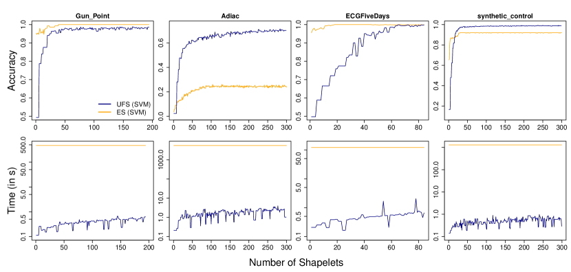
Figure 8: Accuracy achieved and time needed on four different datasets for the exhaustive search (orange) and Ultra-Fast Shapelets (blue), both using a linear SVM for classification.

5.4 Multivariate Datasets

The 15 multivariate datasets used to evaluate Ultra-Fast Shapelets are from various domains such as sign language recognition (AUSLAN), handwriting recognition (CharacterTrajectories, PenDigits), motion (CMU_MOCAP_S16), gesture (uWaveGestureLibrary) and speech recognition (ArabicDigits, JapaneseVowels). Detailed characteristics of the datasets are given in Table 5, detailed results are presented in Table 7. A summary of the empirical evaluation is given in Table 6.

There exist two variations of Ultra-Fast Shapelets: Ultra-Fast Shapelets with ($\nabla$UFS) and without time series derivatives (UFS). Time series derivatives were added since Symbolic Representation for Multivariate Timeseries (SMTS) are using them by default. For SMTS it was shown that this additional information improves the accuracy. Time series derivatives can improve the accuracy for UFS in some cases. In some they do not help, in some they may deteriorate the accuracy since they are adding less helpful predictors. Nevertheless, UFS with derivatives is in 11 out of 15 cases better than without derivatives.

UFS with and without derivatives outperforms the baselines. $\nabla$UFS is for 11, UFS for 10 out of 15 datasets better than SMTS. For NNDTW the number of cases is even 14 or 13, respectively. Comparing UFS to MTSBF, UFS is better in 5 or 6 out of 7 datasets, depending whether time series derivatives are used or not.

Concluding, UFS with derivatives is more accurate than without. UFS is better than SMTS even if no time series derivatives are used and MTSBF has a similar prediction accuracy as SMTS. NNDTW is the worst of the compared classification methods.

Table 5: Characteristics of the multivariate datasets.

Dataset	Train Instances	Test Instances	Streams	Length	Classes
ArabicDigits	6600	2200	13	4-93	10
AUSLAN	1140	1425	22	45-136	95
CharacterTrajectories	300	2558	3	109-205	20
CMU_MOCAP_S16	29	29	62	127-580	2
ECG	100	100	2	39-152	2
JapaneseVowels	270	370	12	7-29	9
Libras	180	180	2	45	15
LP1	38	50	6	15	4
LP2	17	30	6	15	5
LP3	17	30	6	15	4
LP4	42	75	6	15	3
LP5	64	100	6	15	5
PenDigits	300	10692	2	8	10
uWaveGestureLibrary	200	4278	3	315	8
Wafer	298	896	6	104-198	2

Table 6: Summary of empirical evaluation on multivariate time series. (win/lose)

	$\nabla$UFS (RF)	UFS (RF)	SMTS	NNDTW	MTSBF
$\nabla$UFS (RF)	-	11/2	11/4	14/1	6/1
UFS (RF)	2/11	-	10/4	13/1	5/2
SMTS	4/11	4/10	-	13/2	3/3
NNDTW	1/14	1/13	2/13	-	2/5
MTSBF	1/6	2/5	3/3	5/2	-

Table 7: Test error rates averaged over 10 replications for different multivariate time series classification methods compared to Ultra-Fast Shapelets.

Dataset	$\nabla$UFS (RF)	UFS (RF)	SMTS	NNDTW	MTSBF
ArabicDigits	0.033	0.036	0.036	0.092	-
AUSLAN	0.021	0.028	0.053	0.238	0.000
CharacterTrajectories	0.007	0.007	0.008	0.040	0.033
CMU_MOCAP_S16	0.000	0.000	0.003	0.069	0.003
ECG	0.151	0.138	0.182	0.150	0.165
JapaneseVowels	0.056	0.068	0.031	0.351	-
Libras	0.111	0.151	0.091	0.200	0.183
LP1	0.042	0.058	0.144	0.280	-
LP2	0.293	0.307	0.240	0.467	-
LP3	0.213	0.207	0.240	0.500	-
LP4	0.068	0.085	0.105	0.187	-
LP5	0.287	0.296	0.349	0.480	-
PenDigits	0.073	0.081	0.083	0.088	-
uWaveGestureLibrary	0.061	0.071	0.059	0.071	0.101
Wafer	0.013	0.024	0.035	0.023	0.015
Wins	8	4	4	0	1

6 Conclusions

We proposed an ultra-fast way of extracting shapelets motivated by the knowledge of redundant subsequences. Because the shapelet discovery by most authors so far is nothing but a feature subset selection which is costly in time, it was not surprising that our method, Ultra-Fast Shapelets, reduces the runtime by order of magnitudes and is, to the best of our knowledge, the fastest so far published shapelet discovery method.

Furthermore, the ultra-fast shapelet discovery method enabled us to apply shapelet-based classifiers on long univariate datasets as well as on multivariate time series. We compared UFS on 52 univariate datasets with current state-of-the-art shapelet-based methods and showed empirically that it is competitive in terms of accuracy. Additionally, a comparison to state-of-the-art methods for multivariate time series classification on 15 datasets from various domains has shown that Ultra-Fast Shapelets creates predictive features. A Random Forest classifier was better with shapelet features in 11 out of 15 cases compared to SMTS features.

7 Acknowledgements

Partially co-funded by the Seventh Framework Programme of the European Comission, through project REDUCTION (# 288254). www.reduction-project.eu

References

- [1] L. Ye, E. Keogh, Time Series Shapelets: A New Primitive for Data Mining, in: Proceedings of the 15th ACM SIGKDD International Conference on Knowledge Discovery and Data Mining, KDD ’09, ACM, New York, NY, USA, 2009, pp. 947–956.
- [2] J. Hills, J. Lines, E. Baranauskas, J. Mapp, A. Bagnall, Classification of time series by shapelet transformation, Data Mining and Knowledge Discovery 28 (4) (2014) 851–881.
- [3] J. Zakaria, A. Mueen, E. Keogh, Clustering Time Series Using Unsupervised-Shapelets, in: Proceedings of the 2012 IEEE 12th International Conference on Data Mining, ICDM ’12, IEEE Computer Society, Washington, DC, USA, 2012, pp. 785–794.
- [4] M. F. Ghalwash, Z. Obradovic, Early classification of multivariate temporal observations by extraction of interpretable shapelets., BMC Bioinformatics 13 (2012) 195.
- [5] E. J. Keogh, T. Rakthanmanon, Fast Shapelets: A Scalable Algorithm for Discovering Time Series Shapelets., in: SDM, SIAM, 2013, pp. 668–676.
- [6] A. Mueen, E. Keogh, N. Young, Logical-shapelets: An Expressive Primitive for Time Series Classification, in: Proceedings of the 17th ACM SIGKDD International Conference on Knowledge Discovery and Data Mining, KDD ’11, ACM, New York, NY, USA, 2011, pp. 1154–1162.
- [7] K.-W. Chang, B. Deka, W.-M. W. Hwu, D. Roth, Efficient Pattern-Based Time Series Classification on GPU, 2013 IEEE 13th International Conference on Data Mining 0 (2012) 131–140.
- [8] J. Lines, L. M. Davis, J. Hills, A. Bagnall, A Shapelet Transform for Time Series Classification, in: Proceedings of the 18th ACM SIGKDD International Conference on Knowledge Discovery and Data Mining, KDD ’12, ACM, New York, NY, USA, 2012, pp. 289–297.
- [9] J. Grabocka, N. Schilling, M. Wistuba, L. Schmidt-Thieme, Learning Time-Series Shapelets, in: Proceedings of the 20th ACM SIGKDD International Conference on Knowledge Discovery and Data Mining, ACM, 2014.
- [10] B. Hartmann, N. Link, Gesture recognition with inertial sensors and optimized DTW prototypes., in: SMC, IEEE, 2010, pp. 2102–2109.
- [11] S. T., P. B. Sivakumar, Human Gait Recognition and Classification Using Time Series Shapelets, 2012 International Conference on Advances in Computing and Communications 0 (2012) 31–34.
- [12] Q. He, Z. Dong, F. Zhuang, T. Shang, Z. Shi, Fast Time Series Classification Based on Infrequent Shapelets, in: ICMLA (1), 2012, pp. 215–219.
- [13] D. Gordon, D. Hendler, L. Rokach, Fast randomized model generation for shapelet-based time series classification (2012). arXiv:arXiv:1209.5038.
- [14] C. Li, L. Khan, B. Prabhakaran, Real-time classification of variable length multi-attribute motions., Knowl. Inf. Syst. 10 (2) (2006) 163–183.
- [15] X. Weng, J. Shen, Classification of multivariate time series using locality preserving projections, Knowledge-Based Systems 21 (7) (2008) 581–587.
- [16] A. Akl, S. Valaee, Accelerometer-based gesture recognition via dynamic-time warping, affinity propagation, & compressive sensing, in: ICASSP’10, 2010, pp. 2270–2273.
- [17] J. Liu, L. Zhong, J. Wickramasuriya, V. Vasudevan, uWave: Accelerometer-based Personalized Gesture Recognition and Its Applications, Pervasive Mob. Comput. 5 (6) (2009) 657–675.
- [18] M. Baydogan, G. Runger, Learning a symbolic representation for multivariate time series classification, Data Mining and Knowledge Discovery (2014) 1–23
- [19] J. Lin, E. Keogh, L. Wei, S. Lonardi, Experiencing SAX: A Novel Symbolic Representation of Time Series, Data Min. Knowl. Discov. 15 (2) (2007) 107–144.
- [20] I. Guyon, A. Elisseeff, An Introduction to Variable and Feature Selection, J. Mach. Learn. Res. 3 (2003) 1157–1182.
-
[21]
T. Bagnall,