Generalized conditions for genuine multipartite continuous-variable entanglement
Abstract
We derive a hierarchy of continuous-variable multipartite entanglement conditions in terms of second-order moments of position and momentum operators that generalizes existing criteria. Each condition corresponds to a convex optimization problem which, given the covariance matrix of the state, can be numerically solved in a straightforward way. The conditions are independent of partial transposition and thus are also able to detect bound entangled states. Our approach can be used to obtain an analytical condition for genuine multipartite entanglement. We demonstrate that even a special case of our conditions can detect entanglement very efficiently. Using multi-objective optimization it is also possible to numerically verify genuine entanglement of some experimentally realizable states.
pacs:
03.67.Mn, 03.65.Ud, 42.50.DvI Introduction
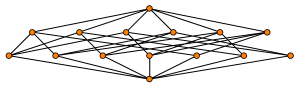
In the multipartite case there are many different notions of entanglement, ranging from the most specific to the most general ones. A specific kind of entanglement means that we precisely specify the groups of parties that are separable from each other, i.e., we specify a partition of the set of indices . A partition is a disjoint set of nonempty subsets of the indices whose union is equal to . For example, in the case there are partitions , and many others. We will use a more compact notation for partitions and write them as and . A partition is finer than a partition (or the partition is coarser than ) if for any there is an such that . For example, the partition is finer than the partition . There are two extreme partitions, the trivial partition and the partition . The former corresponds to the case where no information about separability properties is known and the latter corresponds to the notion of full separability, where all parties are separable from each other. The set of partitions with the finer-than relation is referred to as partition lattice and can be visualized as the graph shown in Fig. 1 for . At the bottom is the trivial partition , then on the second line are all partitions into two parts, next are all partitions into three parts, and so on. At the top is the partition . Partitions with play a special role and are called bipartitions.
From these specific kinds of separability one can construct more general types by considering mixtures of specific kinds according to some criteria. For example, a multipartite state is called -separable, , if it is a mixture of states each of which has separable groups of modes (the corresponding partitions are on the same line in the lattice diagram). In the case of , a -separable state is a state which is a mixture of -, -, -, -, - and -separable states. The notion of -separability of an -partite state is the same as the notion of full separability. A -separable state is referred to as biseparable and the notion of biseparability is the most general of all — a state which is separable in any sense discussed above is automatically biseparable. On the other hand, full separability is the most specific kind of separability — a fully separable state is separable in any other sense.
In general, a biseparable state is a mixture of states corresponding to all nontrivial bipartitions of parties. There are states that cannot be represented as such a mixture. These states, the states that are not biseparable, are called genuine miltipartite entangled. The problem of recognizing which states are genuine entangled is very important for different applications. It is a highly nontrivial task to develop practical conditions for detecting genuine multipartite entanglement. In the following a single party always corresponds to a single electromagnetic mode as known from continuous-variable (CV) quantum information theory Braunstein and van Loock (2005); Weedbrook et al. (2012). Many such conditions for -partite CV systems deal with lower bounds for the second-order quantity
| (1) |
where is the -vector of position and momentum operators and is a real, symmetric, positive definite matrix and is the covariance matrix of the state, . In fact, a special case of matrix with zero off-diagonal blocks is usually used in practice. Denoting and , which are symmetric, positive semidefinite matrices, the quantity in this case reads as
| (2) |
where and are the diagonal blocks of the covariance matrix of the state. For example, the classical result of Ref. Duan et al. (2000) uses rank-one matrices and , where and . The works van Loock and Furusawa (2003); Teh and Reid (2014) use general rank-one matrices and , where and are real -vectors. In Ref. Shchukin and van Loock (2014) the quantity with matrices was used. Refs. Sperling and Vogel (2013); Gerke et al. (2015) deal with the general quantity . Among the works that also use second order moments we mention Hyllus and Eisert (2006); Shalm et al. (2013); Valido et al. (2014). As based on second-order moments only, all these criteria are sufficient entanglement witnesses for all CV states, but necessary and sufficient only for Gaussian states.
In a realistic setting errors of measurements are unavoidable, so to be completely rigorous we need to incorporate the possibility of errors into our scheme. We do this and formulate a hierarchy of entanglement conditions as convex optimization problems for in terms of the covariance matrix and the information about errors of the measurements. For discrete variables a convex optimization approach has been developed in Ref. Eisert et al. (2004).
The paper is organized as follows. In section II we obtain the minimal value of defined by Eq. (2) over all quantum states. In Section III we show how to improve the lower bound obtained in the preceding section for separable states and construct a hierarchy of separability conditions in the form of convex optimization problems. In Section IV we apply our construction to rank one matrices and demonstrate that it coincides with some previously known results, so that those results are just a special case of our more general approach. In Section V we give an example of an entangled state with positive partial transposition that can be detected by our conditions. Section VI is devoted to an analytical condition for genuine multipartite entangled that can be obtained from our hierarchy of conditions. in Section VII we further extend our approach by taking measurement errors into consideration and demonstrating that our method works in realistic settings as well. Then we give a conclusion and provide in appendices all technical details missing in the main part of our work.
II Quantumness bound
First of all, we find the minimum of over all quantum states and then we show how this bound can be improved for separable states. To find the minimal value of for a given matrix we use the Williamson’s theorem *[][p.244]SGQM. This theorem states that there is a symplectic matrix such that , where is a diagonal matrix. Since each symplectic transform is implementable as a unitary transformation Simon et al. (1988), starting with a state we have
| (3) |
for the appropriately transformed state . The minimum of is achieved for being the vacuum state, and in this case the equality takes place. We thus obtain that the inequality is valid for all quantum states and it is tight.
To compute the minimal value of we need to know the diagonal elements of . These numbers are referred to as symplectic spectrum of and they can be directly obtained from the matrix according to the fact that are the eigenvalues of , where and is the identity matrix. In our special case of block-diagonal we can get these numbers directly in terms of and . In fact, we have the equality
| (4) |
The characteristic equation of this matrix is . Since the diagonal blocks commute with the off-diagonal ones, according to *[][p.27; Eq.~(0.8.5.13)]horn-johnson this equation can be simplified as . Substituting the eigenvalues into this equation we see that the diagonal elements satisfy the equation
| (5) |
from which it follows that they are the eigenvalues of the symmetric matrix . The matrices and can be swapped in this derivation. We arrive to the following result: The minimal value of is given by the expression
| (6) |
To put it in another way, we have the tight inequality
| (7) |
which is valid for all positive semidefinite matrices and and all correlation matrices and . This inequality gives some bound on . The bound has been obtained without any assumptions about separability properties of the state in question and thus is valid for all multipartite quantum states. Our task now is to improve this bound for separable states. The improvement will depend on the separability kind of the state — the more separable groups of modes the state has, the higher is its separability kind in the partition lattice and the more can this estimation be improved. In Appendix A we also show that from the inequality (7) one can get a special case of Araki-Lieb-Thirring trace inequalities Lieb and Thirring (1975, 1976); Araki (1990). Such inequalities play some role in quantum entropy theory, see Ref. Ohya and Petz (1993).
III Hierarchy of separability conditions
We first show that pure states with real wave functions are enough to minimize . In fact, in terms of wave functions the quantity reads as
| (8) |
If we take a general wave function of the form , where is a real wave function and is the phase, we will see that the first term in Eq. (8) does not depend on , while the other term is equal to
| (9) |
It follows that for any wave function there is a real wave function (the absolute value of the former) such that and thus we can consider only pure states with real wave functions.
If a pure state with real wave function is -separable then if the indices and belong to different blocks . In fact, separability for pure states means that the wave function is factorizable, i.e., , where, without loss of generality, we can assume that , . For and we have
| (10) |
The fact that is real is important for the validity of the last step. The seeming asymmetry in position and momentum operators is superficial — if we worked in momentum representation and dealt with real wave function in that representation we would have .
We have just shown that if modes and are separable, but for the position correlations we can say only that they factorize: . We can get a similar conclusion for position moments if we take minimization property into account. If a state minimizes then we can also assume that . In fact, taking the wave function , where is the vector of averages computed for the wave function , we get a new wave function with and . If is positive definite then we must have and thus for any separable state that minimizes . If is degenerate then we can just find a separable state with that minimizes , but there can be minimizing states that do not have this property. Moreover, this new wave function also has the property that if and are separable. We see that among -separable states minimizing we can always find a pure state with real wave function for which for , . The notation , where and are sets of indices, is used to denote the submatrix of formed by the intersection of rows with indices in and columns with indices in . Using such a state, we can improve the lower bound for .
Due to the relations for separable and we have the equality
| (11) |
where is obtained from by replacing its elements corresponding to zero elements of by arbitrary real numbers subject to the condition that is symmetric and positive semidefinite and the same procedure is applied to to produce . In other words, we can replace all elements of the submatrices of the form and , , by arbitrary real numbers in such a way that the resulting matrices are again symmetric and positive semidefinite. This construction is better illustrated by an example. For , consider - and -factorizable states. In the former case we have , , and the the latter case we have , , . The matrices corresponding to these two cases are
| (12) |
In the first case we replace elements of the submatrices and by arbitrary numbers, and in the second case we replace submatrices , , , , , . Different submatrices are marked by different colors (symmetric parts are marked by the same color). The more factorizable parts the state has the more elements can be replaced by arbitrary numbers. For a completely factorizable state we can freely choose all the off-diagonal entries.
In order not to overload the notation, we fix some kind of separability, i.e., some decomposition of the indices, and use it in all the considerations below. Applying the inequality (7), we find that for a pure -factorizable state with real wave function, and thus for all -separable states, we have
| (13) |
where the optimization is over the points and such that and are positive definite. For example, for a bipartition with , the vectors and have components, so in this case the optimization problem has variables. The full separability optimization problem has components.
Note that for the vectors and with the corresponding elements of the matrices and , respectively, we have and and thus for any partition . This inequality is strict for most of the matrices and . It follows that the inequality (13) gives a stronger bound on then does the inequality (7). Moreover, in the same way we obtain that if is finer than then , since in this case we have more variables to optimize over, and thus the condition for -separable states gives a stronger bound then the condition for -separability. The condition for full separability gives the strongest bound of all. We have just obtained a hierarchy of separability conditions that mirrors the partition lattice in Fig. 1.
To each kind of separability corresponds its own maximization problem of its own dimension. There are different bipartitions of the indices of an -partite state and many more partitions into three or more parts. If for a given state there is a pair of matrices and such that an inequality (13) is violated, then the state is not -separable. If there are and such that the inequalities (13) are violated for all bipartitions simultaneously, then the state is genuine multipartite entangled.
IV Rank-one matrices
We now show that the results of Ref. van Loock and Furusawa (2003) are just a special case of the general inequalities (13) and give an analytical solution of these optimization problems in this special case. Consider the rank-one matrices and . The square root of a rank-one matrix is given by , so we have . As a concrete example let us consider four-partite case and -separable states. We are free to change some elements of the matrices and . Let us just change the sign of the and ’s elements that are marked in Eq. (12):
| (14) |
For appropriate combinations of signs we can get that and , where the new vectors read as and , and thus
| (15) |
This result can be extended to all and arbitrary kind of separability and coincides with the results obtained in Ref. van Loock and Furusawa (2003).
Note that the inequality is equivalent to the inequalities
| (16) |
The same idea can be applied to the separability conditions and we arrive to the conditions for -separable states
| (17) |
where is a diagonal matrix with diagonal elements equal to so that the elements with indices in the same group have the same sign. These conditions work in many cases, but sometimes the more general conditions are needed. In the next section we give an example of a PPT state that satisfies the inequalities (17) but violates the general inequalities (13).
V An example of PPT state
Consider a four-partite state with the covariance matrix given by Werner and Wolf (2001); Hyllus and Eisert (2006)
| (18) |
The matrix is a covariance matrix of a quantum state, since . Partial transpositions of -kinds (that is transpositions , , and ) are negative, and these negativities are easily detected by the conditions (17). For example, the matrix reads as
| (19) |
and the matrix has negative eigenvalues. On the other hand, the partial transpositions of -kinds are all positive and the matrices (17) with are positive semidefinite, so the test (17) does not detect any entanglement of a -kind. Nevertheless, the state (18) is entangled in any of this kind.
To demonstrate this, consider the positive semidefinite matrices
| (20) |
where , , and are some positive numbers to be determined. The quantity reads as . To compute , note that
| (21) |
where the matrices and are defined to be (since we can play with the elements marked by color)
| (22) |
and thus for the boundary we have the inequality
| (23) |
It is easy to check that for the following values of the parameters:
| (24) |
we have , while according to Eq. (23) we have . We see that , and the PPT state Eq. (18) is -entangled. The construction for the partitions and is similar.
VI Genuine entanglement condition
The inequalities (13) allow one to test states for entanglement of some kind, but the number of these kinds grows extremely fast with the number of parts. We now derive an analytical condition for genuine multipartite entanglement. It is a single condition that does not require testing exponentially many bipartitions, however, it does not provide the best possible bound. Consider the quantity
| (25) |
It is the general quantity with the following matrices and :
| (26) |
Since matrices and are completely symmetric with respect to different parts, it is enough to consider only bipartitions of the form for . We do not change the elements of , and in the matrix we set all to (so we change the matrix elements from to ). Denote the resulting matrix by . The matrices and commute, so that is easy to compute
| (27) |
where the number is given by
| (28) |
The minimum of this expression over is attained for . We have just obtained the following result: Any biseparable state must satisfy the inequality
| (29) |
If this inequality is violated, then the state is genuine multipartite entangled. Table 1 summarizes the lower bounds of for some obtained with the analytical condition (29) and computed numerically from Eq. (13).
| 3 | 4 | 5 | 6 | 7 | 8 | ||
|---|---|---|---|---|---|---|---|
| q | |||||||
| a | |||||||
| b | |||||||
| f |
A similar genuine entanglement condition has been obtained in Ref. van Loock and Furusawa (2003) in terms of rank-one matrices. The gap between quantum bound and biseparability bound there decreases as , where is the number of parts111In fact, in Ref. van Loock and Furusawa (2003) the term genuine entanglement was used in a different, weaker, sense. But the condition obtained there happens to work for genuine entanglement in the present, stronger, sense.. In our condition this gap is and so it does not tend to zero for large .
VII Convex optimization and experimental errors
To demonstrate entanglement of a kind we need to find a pair of matrices and that violate the condition (13). In practice, however, we should take into account the errors in the measurement of the matrix elements of and . Assuming that the errors in the individual elements of and are independent, the standard deviation of is given by the expression
| (30) |
where and are the standard deviations of individual elements of and respectively. So, to be on the safe side the right inequality reads as
| (31) |
where is the level of certainty with which we can claim that the state is entangled. We prove that the function is convex on the set of all pairs of semidefinite matrices .
To prove the convexity of we have to prove the concavity of because the convexity of the other two terms of is obvious. The key element of this proof is the fact that is jointly concave with respect to all four variables , , and . Due to the equality
| (32) |
it immediately follows is concave with respect to and as the minimum of a family of concave (in fact, linear) functions. From the relation
| (33) |
, and similar relation for we derive the joint concavity of .
We now have three sets — the set of points where and are positive definite, the similar set for and , and the set for and . In general, these are distinct sets, but one can easily see that . The standard argument given in Ref. Boyd and Vandenberghe (2004) can be applied here to conclude that is concave as the maximum of a jointly concave function over a convex set. This finishes the proof of the convexity of the function defined by Eq. (31).
To violate the inequality (31) we thus have to optimize over and and check whether the optimal value is negative or not. This optimization problem has variables, the elements of and . Since the function is homogeneous, for , it makes sense to put some condition on the matrices and . The simplest is a linear condition, for example, the condition , where is an arbitrary fixed positive constant. We thus arrive to the following -separability condition:
| (34) |
If, for given , , and , this inequality is violated, i.e., if this minimum drops below then the state in question is not separable of the corresponding kind. If these inequalities can be violated for all bipartitions simultaneously (by the same pair of matrices and ), then the state is genuine multipartite entangled. The methods to solve convex optimization problems like the one given by Eq. (34) are discussed, e.g, in Ref. Boyd and Vandenberghe (2004).
What should we choose? Usually, the ”three-sigma rule”, is applied Grafarend (2006). To better understand what values of in Eq. (31) are sufficient to guarantee that our results are correct we need to know the probability that the result of a measurement lies outside sigma interval. For a Gaussian probability distribution with the mean and the standard deviation this probability is given by the expression
| (35) |
which depends only on . This probability decreases very quickly as growth. The order of values of for some are shown in the table below.
| 1 | 2 | 3 | 4 | 5 | 6 | 7 | 10 | |
|---|---|---|---|---|---|---|---|---|
In many cases, the value of is sufficient (the three-sigma rule). For this probability is negligible, and for it is practically zero. Even if the real probability distribution is not perfectly Gaussian it is unlikely to have long tail, so Eq. (35) gives a reasonable estimate. Even if this estimate is wrong by several orders of magnitude, provided that we have verified violation with we are still on the safe side. The larger we set the larger the probability of the correct result is, but the more difficult it will be to find a violation with such . From this table we can conclude that we should search for a violation with not smaller than 3 and not larger than 6 — the event of getting the right result outside of six sigma interval is practically impossible.
We see that if we can violate our inequalities with then it practically guarantees that our conclusion is correct. In Appendix B we demonstrate the usefulness of our approach by applying to some four-, six- and ten-partite realistic states. We also demonstrate that the four-partite state in question is genuine multipartite entangled.
VIII Conclusion
We have developed a method to test continuous-variable multipartite states for arbitrary kinds of entanglement. Our approach allows both numerical and analytical treatment. Numerically, it reduces to a convex optimization problem, which allows fast and accurate solution. We have shown that it is very efficient at detecting ordinary entanglement and can detect genuine multipartite entanglement in a reasonable amount of time. Analytically, it allows to reproduce (and thus generalize) some known results as well as to obtain an analytical genuine multipartite entanglement condition. With our approach we can easily obtain a trace-class inequality, which is difficult to get in a direct way.
Appendix A Trace inequalities
If matrices and commute then the right-hand side of Eq. (6) reduces to . This expression, , is a lower bound for independent of commutation properties of and . For a real wave function we have the equality
| (36) |
where the vector fields and are defined via and . We can write this equality in a more compact form as
| (37) |
where the new vector fields are defined via and . Now we can estimate as follows:
| (38) |
From the relation
| (39) |
we get the inequality .
We thus have two lower bounds for — the tight one is given by the inequality (6) and the other one, not necessarily tight, have just been obtained with the help of Cauchy-Schwarz inequality. Since the tight bound is the best bound possible, we derive the following inequality for a pair of positive definite matrices and :
| (40) |
This inequality is a special case of Araki-Lieb-Thirring trace inequalities Lieb and Thirring (1975, 1976); Araki (1990), which also have quantum mechanical background and read as
| (41) |
where and are arbitrary positive definite matrices, and . The case of and corresponds to the inequality (40).
Appendix B Application to realistic matrices
It happens that rank-one matrices work surprisingly well. Consider the four-partite state that was analyzed in Ref. Gerke et al. (2015). It has the following covariance matrix:
| (42) |
The standard deviation matrix reads as
| (43) |
A very simple way to search for violation of the condition (31) is to randomly generate 4-vectors and and check whether this condition is violated by the rank-one matrices and , and if it is, how strong the violation is. Then just record the maximal observed violation. As a measure of violation we use the quantity
| (44) |
This approach requires only simple matrix algebra manipulations, which can be done very efficiently with tools like Intel Math Kernel Library. A simple parallel Fortran program has been written and run on a low-end 4-core desktop PC. The total time to test all seven possible bipartitions in this four-partite case is 4 minutes (using all four cores available). Table 2 compares our results with those obtained in Ref. Gerke et al. (2015). We see that for the state under study our approach is superior to that of Ref. Gerke et al. (2015) (which uses a genetic algorithm to find the best violation), since it is simpler and gives better results, though, as we have mentioned before, from practical point of view all violations larger than 6 are of the same value.
| Bipart. | Violation | ||
|---|---|---|---|
| Ref. Gerke et al. (2015) | 4m | ||
| 20.93 | 26.48 | ||
| 13.17 | 18.08 | ||
| 11.21 | 16.10 | ||
| 21.06 | 26.57 | ||
| 24.34 | 27.79 | ||
| 23.52 | 26.17 | ||
| 4.66 | 9.72 | ||
We now apply our technique to the six-partite state also considered in Ref. Gerke et al. (2015). We have performed two runs of our program on the same hardware as in the previous case, one with a smaller number of random trials and the other with 200 times more trials. The first run takes approximately 4 minutes to perform all 31 tests, the other one takes around 12 hours. As Table. 3 demonstrates, in this case the optimization based on a genetic algorithm gives somewhat larger violations. On the other hand, we do not know what computational resources were used to perform that optimization and how much time it took. As we have already said, all violation larger than 6 are of the same practical value and our method produced much better violations in just a few minutes on a low-end PC.
| Bipartition | Violation | ||
|---|---|---|---|
| Ref. Gerke et al. (2015) | 12h | 4m | |
The last state considered in Ref. Gerke et al. (2015) is a ten-partite state. It has been reported that the smallest violation of 1.1 was obtained for the bipartition . The corresponding probability to get wrong result is , and it is not small enough to conclude that the state under study is not -separable. Randomly generating vectors and , we have found that the inequality (31) for this kind of separability can be violated with . The corresponding probability is much smaller and gives a strong confidence that the state is -entangled. The vectors are
| (45) |
The violations of other kinds of biseparability are all larger than 3, so the standard three-sigma test is passed for all bipartitions. The violations reported in Ref. Gerke et al. (2015) show some strange behavior — the violation for full separability is smaller than violations of some more coarse kinds. But this may be an artifact of an implementation of the genetic optimization algorithm.
Up to now it has been shown that the four-partite state with the covariance matrix (42) is not separable for any fixed kind of separability. We demonstrate that this state is genuine entangled. To do this we need to find a pair of matrices and that simultaneously violate the inequalities (31) for all bipartitions. First, we have tried to violate these inequalities with rank-one matrices. It took nearly one day, but we were able to find a pair of vectors
| (46) |
that violate the conditions (31) for all seven bipartitions, and the minimal violation is (for the bipartition ). The corresponding probability is relatively small to conclude that the state under study is genuine entangled.
The approach with a simpler conditions works but it takes a lot of time and it just marginally passes the three-sigma test. Using the general matrices we can do better. The sketch of our approach is as follows. We use a variant of the steepest gradient method. According to this method, to optimize a convex function one has to go in the direction opposite to the gradient of the function. Here we have several functions to be optimized at once, and each has its own gradient. We start by generating a pair of random positive definite matrices and and compute the gradients of all seven target functions. If the directions of these gradients are not strongly scattered then we can take the average of the gradients, go in the opposite direction and still improving all our functions simultaneously. If the gradients point into nearly opposite directions then we cannot proceed this way, so we stop and generate a new random pair of matrices. We do this until we find proper matrices and or give up after some prescribed number of attempts. Following this approach, in a few hours we found the following pair of matrices for the four-partite state with the covariance matrix (42):
For these matrices we have and . The bound for different bipartitions is presented below. The elements of the matrices that were optimized over are highlighted. For the bipartition the maximum is attained at
and is equal to . For the bipartition at
and is equal to . For the bipartition at
and is equal to . For the bipartition at
and is equal to . For the bipartition at
and is equal to . For the bipartition at
and is equal to . For the bipartition at
and is equal to . The smallest number among these maximums is the last one, , so we have
for all bipartitions simultaneously. The corresponding probability is , which is almost two orders of magnitude smaller than for the vectors and we found before, so one can be pretty sure that the state under study is genuine entangled.
References
- Braunstein and van Loock (2005) S. L. Braunstein and P. van Loock, Rev. Mod. Phys. 77, 513 (2005).
- Weedbrook et al. (2012) C. Weedbrook, S. Pirandola, R. García-Patrón, N. J. Cerf, T. C. Ralph, J. H. Shapiro, and S. Lloyd, Rev. Mod. Phys. 84, 621 (2012).
- Duan et al. (2000) L.-M. Duan, G. Giedke, J. I. Cirac, and P. Zoller, Phys. Rev. Lett. 84, 2722 (2000).
- van Loock and Furusawa (2003) P. van Loock and A. Furusawa, Phys. Rev. A 67, 052315 (2003).
- Teh and Reid (2014) R. Y. Teh and M. D. Reid, Phys. Rev. A 90, 062337 (2014).
- Shchukin and van Loock (2014) E. Shchukin and P. van Loock, Phys. Rev. A 90, 012334 (2014).
- Sperling and Vogel (2013) J. Sperling and W. Vogel, Phys. Rev. Lett. 111, 110503 (2013).
- Gerke et al. (2015) S. Gerke, J. Sperling, W. Vogel, Y. Cai, J. Roslund, N. Treps, and C. Fabre, Phys. Rev. Lett. 114, 050501 (2015).
- Hyllus and Eisert (2006) P. Hyllus and J. Eisert, New Journal of Physics 8, 51 (2006).
- Shalm et al. (2013) L. K. Shalm, D. R. Hamel, Z. Yan, C. Simon, K. J. Resch, and T. Jennewein, Nat. Phys. 9, 19 (2013).
- Valido et al. (2014) A. A. Valido, F. Levi, and F. Mintert, Phys. Rev. A 90, 052321 (2014).
- Eisert et al. (2004) J. Eisert, P. Hyllus, O. Gühne, and M. Curty, Phys. Rev. A 70, 062317 (2004).
- de Gosson (2006) M. A. de Gosson, Symplectic Geometry and Quantum Mechanics (Birkhäuser, 2006).
- Simon et al. (1988) R. Simon, E. C. G. Sudarshan, and N. Mukunda, Phys. Rev. A 37, 3028 (1988).
- Horn and Johnson (2013) R. A. Horn and C. R. Johnson, Matrix Analysis, 2nd ed. (Cambridge University Press, 2013).
- Lieb and Thirring (1975) E. H. Lieb and W. E. Thirring, Phys. Rev. Lett. 35, 687 (1975).
- Lieb and Thirring (1976) E. H. Lieb and W. E. Thirring, in Studies in Mathematical Physics, edited by E. Lieb, B. Simon, and A. Wightman (Princeton University Press, 1976) pp. 269–303.
- Araki (1990) H. Araki, Lett. Math. Phys. 19, 167 (1990).
- Ohya and Petz (1993) M. Ohya and D. Petz, Quantum entropy and its use (Springer-Verlag, 1993).
- Werner and Wolf (2001) R. F. Werner and M. M. Wolf, Phys. Rev. Lett. 86, 3658 (2001).
- Note (1) In fact, in Ref. van Loock and Furusawa (2003) the term genuine entanglement was used in a different, weaker, sense. But the condition obtained there happens to work for genuine entanglement in the present, stronger, sense.
- Boyd and Vandenberghe (2004) S. Boyd and L. Vandenberghe, Convex Optimization (Cambridge University Press, 2004).
- Grafarend (2006) E. W. Grafarend, Linear and Nonlinear Models: Fixed Effects, Random Effects, and Mixed Models (Walter de Gruyter, 2006).