A Linear-Time Algorithm for Finding All Double-Vertex Dominators of a Given Vertex

Abstract

Dominators provide a general mechanism for identifying reconverging paths in graphs. This is useful for a number of applications in Computer-Aided Design (CAD) including signal probability computation in biased random simulation, switching activity estimation in power and noise analysis, and cut points identification in equivalence checking. However, traditional single-vertex dominators are too rare in circuit graphs. In order to handle reconverging paths more efficiently, we consider the case of double-vertex dominators which occur more frequently. First, we derive a number of specific properties of double-vertex dominators. Then, we describe a data structure for representing all double-vertex dominators of a given vertex in linear space. Finally, we present an algorithm for finding all double-vertex dominators of a given vertex in linear time. Our results provide an efficient systematic way of partitioning large graphs along the reconverging points of the signal flow.

raph, dominator, min-cut, logic circuit, reconverging path

1 Introduction

This paper considers the problem of finding dominators in circuit graphs. A vertex $v$ is said to dominate another vertex $u$ if every path from $u$ to the output of the circuit contains $v$ [1]. For example, for the circuit in Figure 1(a), vertex $n$ dominates vertex $e$; vertex $p$ dominates vertex $h$, etc.

Dominators provide a general mechanism for identifying re-converging paths in graphs. If a vertex $v$ is the origin of a re-converging path, then the immediate dominator of $v$ is the earliest point at which such a path converges. For example, in Figure 1(a), the re-converging path originated at $e$ ends at $n$; the re-converging path originated at $g$ ends at $f$.

Knowing the precise starting and ending points of a re-converging path is useful in a number of applications including computation of signal probabilities in biased random simulation, estimation of switching activities in power and noise analysis, and identification of cut points in equivalence checking.

The signal probability of a net in a combinational circuit is the probability that a randomly generated input vector will produce the value one on this net [2]. Signal probability analysis is used, for example, to measure and control the coverage of vector generation for biased random simulation [3].

The average switching activity in a combinational circuit is the probability of its net values to change from 0 to 1 or vice verse [4]. It correlates directly with the average dynamic power dissipation of the circuit, thus its analysis is useful for guiding logic optimization methods targeting low power consumption [5].

Computation of signal probabilities and switching activities based on topologically processing the circuit from inputs to outputs and evaluating the gate functions generally produces incorrect results due to higher-order exponents introduced by correlated signals [2]. For example, if the functions $f$ and $g$ have variables in common, then $P[f\wedge g]\not=P[f]\cdot P[g]$, where $P$ is the signal probability. Dominators provide the earliest points during topological processing at which all signals correlated with signal originated at the dominated vertex converge. Therefore, the computation of signal probabilities and switching activities can be partitioned along the dominator points.

Cut-points based equivalence checking partitions the specification and implementation circuits along frontiers of functionally equivalent signal pairs, called cut-points [6]. This is usually done in four steps: (1) cut-points identification, attempting to discover as many cut-points as possible, (2) cut-points selection, aiming to choose the cut-points which simplify the task of verification, (3) equivalence checking of the resulting sub-circuits, (4) false negative reduction. Dominators provide a systematic mechanism for identifying and choosing good cut-points in circuits, since converging points of the signal flow are ideal candidates for cut-points.

In spite of the theoretical advantages of dominators, previous attempts to apply dominator-based techniques to large circuits have not been successful. Two main reasons for this are: (1) single-vertex dominators, which can be found in linear time, are too rare in circuits; (2) multiple-vertex dominators, which are common in circuits, require exponential time to be computed. In other words, no systematic approach for finding useful dominators in large circuits efficiently has been known so far. Useful are normally dominators of a small size because $2^{k}$ combinations of values of a $k$-vertex dominator have to be manipulated to resolve signal correlations [7].

In this paper, we focus on the specific case double-vertex dominators. First, we prove a number of fundamental properties of double-vertex dominators. For example, we show that immediate double-vertex dominators are unique. This property also holds for single-vertex dominators, but it does not extend to dominators of size larger than two. Then, we present a data structure for representing all double-vertex dominators of a given vertex in linear space. Finally, we introduce an algorithm for finding all double-vertex dominators of a given vertex in linear time. This asymptotically reduces the complexity of the previous quadratic algorithm for finding double-vertex dominators [8].

The paper is organized as follows. Section 2 presents basic notation and definitions. In Section 3, we introduce definitions of dominators which are more general than the traditional ones from [1]. Section 4 summarizes the previous work on dominators. In Sections 5 and 6, we describe properties of multiple-vertex and double-vertex dominators, respectively. Section 7 presents the data structure for representing double-vertex dominators. Section 9 describes the new algorithm for finding double-vertex dominators. The experimental results are shown in Section 10. Section 11 concludes the paper.

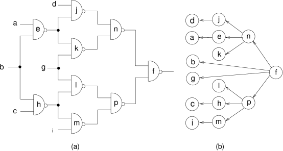
Figure 1: (a) An example circuit; (b) Its dominator tree.

2 Preliminaries

Unless otherwise specified, throughout the paper, we use capital letters $A,B,C,$ etc. to denote vectors and bold letters $\mathbb{A},\mathbb{B},\mathbb{C},$ etc. to denote sets.

Let $G=(\mathbb{V},\mathbb{E},root)$ denote a single-output acyclic circuit graph where the set of vertices $\mathbb{V}$ represents the primary inputs and gates. A particular vertex $root\in\mathbb{V}$ is marked as the circuit output. The set of edges $\mathbb{E}\subseteq\mathbb{V}\times\mathbb{V}$ represents the nets connecting the gates.

Fanin and fanout sets of a vertex $v\in\mathbb{V}$ are defined as $fanin(v)=\{u\ |(u,v)\in E\}$ and $fanout(v)=\{u\ |(v,u)\in E\}$, respectively.

The transitive fanin of a vertex $v\in\mathbb{V}$ is a subset of $\mathbb{V}$ containing all vertices from which $v$ in reachable. Similarly, the transitive fanout of a vertex $v\in\mathbb{V}$ is a subset of $\mathbb{V}$ containing all vertices reachable from $v$.

A path $P=(v_{1},v_{2},\ldots,v_{|P|})$ is a vector of vertices of $\mathbb{V}$ such that $(v_{i},v_{i+1})\in\mathbb{E}$ for all $i\in\{1,\ldots,|P|-1\}$. The vertices $v_{1}$ and $v_{|P|}$ are called the source and the sink of $P$, respectively. The source and the sink of $P$ are called the terminal vertices of $P$. The remaining vertices of $P$ are called the non-terminal vertices.

Throughout the paper, we call two paths disjoint if the intersection of sets of their non-terminal vertices is empty.

Given two paths $P_{1}=(v_{1},v_{2},\ldots,v_{|P_{1}|})$ and $P_{2}=(w_{1},w_{2},\ldots,w_{|P_{2}|})$, the concatenation of $P_{1}$ and $P_{2}$ is defined only if $v_{|P_{1}|}=w_{1}$. The result of the concatenation is the path $P_{3}=(v_{1},v_{2},\ldots,v_{|P_{1}|},w_{2},\ldots,w_{|P_{2}|})$. We use the notation $P_{3}=P_{1}P_{2}$ to denote that $P_{3}$ is a concatenation of $P_{1}$ and $P_{2}$.

A prefix of a vertex $P$, denoted by prefix$(P)$, is a sub-vertex of $P$ containing $k$ first adjacent vertices of $P$ for some $1\leq k<|P|$. A suffix of a vertex $P$, denoted by suffix$(P)$, is a sub-vertex of $P$ containing $k$ last adjacent vertices of $P$ for some $1<k\leq|P|$.

3 Definition of Dominators

In this section, we introduce definitions of dominators and immediate dominators which are more general than the traditional ones from [1].

Definition 1

A set of vertices $\mathbb{A}$ dominates a set of vertices $\mathbb{B}$ with respect to a set of vertices $\mathbb{C}$ if every path which starts at a vertex in $\mathbb{B}$ and ends at a vertex in $\mathbb{C}$ contains at least one vertex from $\mathbb{A}$.

Definition 2

A set of vertices $\mathbb{A}$ is a dominator of a set of vertices $\mathbb{B}$ with respect to a set of vertices $\mathbb{C}$, if

• $\mathbb{A}$ dominates $\mathbb{B}$,

• $\forall v\in\mathbb{A}$, $\mathbb{A}-\{v\}$ does not dominate $\mathbb{B}$.

The sets $\mathbb{B}$ and $\mathbb{C}$ are called, the source set and the sink set, respectively. For example, for the circuit in Figure  1(a), $\{j,k,l\}$ is a dominator of the source $\{e,g\}$ with respect to the sink $\{n,p\}$.

In most applications of dominators, the source set $\mathbb{B}$ and the sink set $\mathbb{C}$ are known, while the dominator set $\mathbb{A}$ needs to be computed. The sizes of the sets $\mathbb{B}$, $\mathbb{C}$ are neither important for the choice of data structure for representing dominators, nor for the algorithm which finds them. Vertices in the set $\mathbb{B}$ can be merged into a single vertex $v_{b}$ which feeds all the vertices fed by any vertex in $\mathbb{B}$. Similarly, vertices into the set $\mathbb{C}$ can be merged to a single vertex $v_{c}$ which is fed by all vertices feeding any vertex in $\mathbb{C}$. In this case finding a dominator for $v_{b}$ with respect to $v_{c}$ is equivalent to finding a dominator for $\mathbb{B}$ with respect to $\mathbb{C}$. Therefore, an algorithm which handles the case $|\mathbb{B}|=|\mathbb{C}|=1$ can be extended to the sets $\mathbb{B}$ and $\mathbb{C}$ of an arbitrary size.

Contrary, the size of the dominator set $\mathbb{A}$ is crucial for the choice of data structures and algorithms. Therefore, the size of $\mathbb{A}$ is the most important criteria for characterizing the properties of a dominator. We use the term $k$-vertex dominator to refer to the case of $|\mathbb{A}|=k$. If $k>1$ then we may also call a $k$-vertex dominator multiple-vertex dominator. If a dominator dominates more then one vertex, i.e. $|B|>1$, it is called common $k$-vertex dominator.

Throughout this paper, unless specified otherwise, the vertex $root$ is assumed to be the sink for any considered dominator relation. So, if we say that $\mathbb{A}$ dominates $\mathbb{B}$, we mean that $\mathbb{A}$ dominates $\mathbb{B}$ with respect to $root$.

Definition 3

A set of vertices $\mathbb{A}$ is a strict dominator of a set of vertices $\mathbb{B}$, if $\mathbb{A}$ is a dominator of $\mathbb{B}$ and $A\bigcap B=\emptyset$.

For example, in Figure  1(a), $\{j,k,h\}$ is a dominator of $\{b,h\}$, but it is not strict. On the other hand, $\{j,k,h\}$ is a strict dominator of $\{b\}$. Obviously, any dominator of a single vertex is a strict dominator. All results in this paper are derived for dominators of single vertices. Therefore, throughout the paper when we write ”dominator” it also means ”strict dominator”. Note that any algorithm which finds only strict dominators can be extended to find all dominators by introducing a fake vertex which feeds all nodes in $\mathbb{B}$. The search is carried out with the fake vertex constituting the new $\mathbb{B}$.

Definition 4

A set $\mathbb{A}$ is an immediate $k$-vertex dominator of a set $\mathbb{B}$ if $\mathbb{A}$ is a strict $k$-vertex dominator of $\mathbb{B}$ and $\mathbb{A}$ does not dominate $\mathbb{D}$, where $\mathbb{D}$ is any other strict $k$-vertex dominator of $\mathbb{B}$.

The concept of immediate dominators has a special importance for single-vertex dominators. It was shown in [9, 10] that every vertex $v$ in a directed acyclic graph $G$ except $root$ has a unique immediate single-vertex dominator, $idom(v)$. The edges $\{(idom(v),v)\ |\ v\in\mathbb{V}-\{root\}\}$ form a directed tree rooted at $root$, which is called the dominator tree of $G$. For example, the dominator tree for the circuit in Figure 1(a) is shown in Figure 1(b).

Note that the immediate multiple-vertex dominators are not necessarily unique. For example, vertex $b$ in Figure 1(a) has two immediate 3-vertex dominators: $\{j,k,h\}$ and $\{e,l,m\}$. Later in the paper we prove that the immediate dominators are always unique for the case of $k=2$.

It might be worth mentioning that dominators are more general than min-cut in circuit partitioning [11]. A min-cut is required to dominate all vertices in its transitive fanin. Therefore, every min-cut is a dominator, but not every dominator is a min-cut.

4 Previous Work

The problem of finding single-vertex dominators was first considered in global flow analysis and program optimization. Lorry and Medlock [9] presented an $O(n^{4})$ algorithm for finding all immediate single-vertex dominators in a flowgraph with $n$ vertices. Successive improvements of this algorithm were done by Aho and Ullman [10], Purdom and Moore [12], and Tarjan [13], culminating in Lengauer and Tarjan’s [1] $O(e\alpha(e,n))$ algorithm, where $e$ is the number of edges and $\alpha$ is the standard functional inverse of the Ackermann function which grows slowly with $e$ and $n$.

The asymptotic time complexity of finding single-vertex dominators was reduced to linear by Harel [14], Alstrup et al. [15] and Buchsbaum et al. [16]. However, these improvements in asymptotic complexity did not contribute much to reducing the actual runtime. For example, the algorithm [16] runs 10% to 20% slower than Lengauer and Tarjan’s [1]. Lengauer and Tarjan algorithm appears to be the fastest of algorithms for single-vertex dominators on graphs of large size.

One of the first attempts to develop an algorithm for the identification of multiple-vertex dominators was done by Gupta. In [17], three algorithms addressing this problem were proposed. The first finds all immediate multiple-vertex dominators of size up to $k$ in $O(n^{k})$ time. Computing immediate dominators is easy because an immediate dominator of a vertex $v$ is always contained in the set of fanout vertices of $v$. Possible redundancies can be removed by checking whether for every $u$ in the fanout of $v$ there exists at least one path from $u$ to $root$ which contains $u$ and does not contain any other $w$ in the fanout of $v$.

The second algorithm in [17] finds all multiple-vertex dominators of a given vertex. The number of all dominators of a vertex can be exponential with respect to $n$. Since the algorithm represents each dominator explicitly as a set of vertices, it has exponential space and time complexity.

The third algorithm in [17] finds all multiple-vertex dominators of size up to $k$ for all vertices in the circuit. Due to its specific nature, this algorithm cannot not be modified to search for all multiple-vertex dominators of a fixed size for a given vertex. The complexity of the algorithm is not evaluated in the paper. Depending on the implementation, the complexity can vary from exponential to polynomial with a high degree of the polynomial. For example, for double-vertex dominators, the complexity of the algorithm is at least $O(n^{5})$.

Successive improvements of the algorithms in [17] were done in [18, 19, 20] and [21]. The algorithm presented in [21] finds the set of all possible $k$-vertex dominators of a circuit by iteratively restricting the graph with respect to one of its vertices, $v$. The restriction is done by removing from the graph all vertices dominated by $v$. Dominators of size $k-1$ are then computed for the resulting restricted graph by applying the same technique recursively. Once $k$ is reduced to 1, a single-vertex dominator algorithm is used. Since single-vertex dominators can be computed in linear time, the overall complexity of the algorithm [21] is bounded by $O(n^{k})$.

The first algorithm designed specifically for double-vertex dominator was presented in [8]. This algorithm uses the max-flow algorithm to find an immediate double-vertex dominator for a given set of vertices $\mathbb{B}$. The immediate dominator is considered as a sink and all vertices in $\mathbb{B}$ are merged into a single source vertex. The obtained min-cut corresponds to the minimal-size dominator which dominates all paths from the source to the sink. If the size of the min-cut is larger than two, then $S$ does not have any double-vertex dominators. The complexity of this algorithm is $O(n^{2})$.

Interesting results on testing two-connectivity of directed graphs in linear time were presented in [22], with a focus on finding disjoint paths. Since dominators are contained in disjoint paths, the results of [22] can potentially facilitate their search. However, with such an approach, the complexity of checking if a pair of vertices is a double-vertex dominator remains linear. As we show later, in our case it is reduced to a constant.

The cactus tree data structure for representing all undirected min-cuts was introduced in [23]. The problem of finding a min-cut of a high degree is reduced to finding a two-element cut in the cactus tree. Such a structure allows for extracting min-cuts of a high degree, which are a special case of $k$-vertex dominators. In our case, the original degree is two. Therefore, the cactus tree data structure cannot help reduce is further.

5 Properties of Multiple-Vertex Dominators

In this section, we derive some general properties of $k$-vertex dominators. The following three Lemmata show antisymmetry, transitivity, and reflexivity of the dominator relation.

Lemma 1

Let $\mathbb{A}$ and $\mathbb{B}$ be two different dominators of a vertex $u$. If $\mathbb{B}$ dominates $\mathbb{A}$, then $\mathbb{A}$ does not dominate $\mathbb{B}$.

Proof: Set $\mathbb{A}$ is not equal to $\mathbb{B}$ by the condition of the Lemma. $\mathbb{A}$ is not a proper subset of $\mathbb{B}$ either, because otherwise $\mathbb{B}$ would violate the Definition 2b. Thus, there is a vertex $v\in A$ such that $v\not\in B$. Since $\mathbb{A}$ is a dominator of $u$, by Definition 2b, there exists $P=(u,\ldots,root)$, such that $v\in P$, and $v_{2}\not\in P$, $\forall v_{2}\in(A-\{v\})$. The path $P_{2}=(v,\ldots,root)$ which is suffix of $P$ should contain a vertex $w\in B$ since $\mathbb{B}$ dominates $\mathbb{A}$. The path $P_{3}=(w,\ldots,root)$ which is a suffix of $P_{2}$ does not contain any vertex of $\mathbb{A}$ by construction. Thus, by Definition 1, $\mathbb{B}$ does not dominate $\mathbb{A}$.

$\Box$

Lemma 2

If $\mathbb{A}$ dominates $\mathbb{B}$ and $\mathbb{B}$ dominates $\mathbb{C}$, then $\mathbb{A}$ dominates $\mathbb{C}$.

Proof: Consider an arbitrary path $P=(v,\ldots,root)$ such that $v\in\mathbb{C}$. We proof the Lemma by showing that a vertex from $\mathbb{A}$ is in $P$. Since $\mathbb{B}$ dominates $\mathbb{C}$, it holds that $\exists w\in B$ such that $w\in P$. The path $P_{2}=(w,\ldots,root)$ is a suffix of $P$. Since $\mathbb{A}$ dominates $\mathbb{B}$, it holds that $\exists u\in A$ such that $u\in P_{2}$. Thus $u\in P$ as well.

$\Box$

Lemma 3

$\mathbb{A}$ dominates $\mathbb{A}$.

Proof: Follows trivially from the Definition 1a.

$\Box$

It follows from the above three Lemmata that any set of dominators of a vertex $u$ is partially ordered by the dominator relation.

6 Properties of Double-Vertex Dominators

In this section, we derive a number of fundamental properties of double-vertex dominators.

Let $\mathbb{D}_{u}$ be the set of all possible double-vertex dominators of a vertex $u\in\mathbb{V}$. Each element of $\mathbb{D}_{u}$ is a pair of vertices $\{v,w\}$, $v,u\in\mathbb{V}$, constituting a double-vertex dominator of $u$. With some abuse of notation, throughout the paper we write $v\in\mathbb{D}_{u}$ as a shorthand for $\exists w\in\mathbb{V}$ such that $\{v,w\}\in\mathbb{D}_{u}$.

The following Lemma shows that if two dominators have a common vertex, then one of the dominators dominates the non-common vertex in another dominator.

Lemma 4

If $\{v_{1},v_{2}\}\in\mathbb{D}_{u}$ and $\{v_{2},v_{3}\}\in\mathbb{D}_{u}$, then either $\{v_{1},v_{2}\}$ dominates $v_{3}$, or $\{v_{2},v_{3}\}$ dominates $v_{1}$.

Proof: If $\{v_{1},v_{2}\}$ dominates $v_{3}$, then the Lemma holds trivially. Suppose that $\{v_{1},v_{2}\}$ does not dominate $v_{3}$. Since $\{v_{2},v_{3}\}\in\mathbb{D}_{u}$, by Definition 2b, there exists $P_{1}=(u,\ldots,root)$, such that $v_{3}\in P_{1}$ and $v_{2}\not\in P_{1}$. Since $\{v_{1},v_{2}\}\in\mathbb{D}_{u}$, for all $P_{1}$ it holds that $v_{1}\in P_{1}$. Furthermore, $v_{1}$ precedes $v_{3}$ in $P_{1}$, because, by assumption, $\{v_{1},v_{2}\}$ does not dominate $v_{3}$. Thus the prefix $P_{2}=(u,\ldots,v_{1})$ of the path $P_{1}$ does not contain $v_{2}$ and $v_{3}$.

Then, there exists no path $P_{3}=(v_{1},\ldots,root)$ such that $v_{2},v_{3}\not\in P_{3}$, because otherwise the path $P_{2}P_{3}$ would contain neither $v_{2}$ nor $v_{3}$. This would contradict $\{v_{2},v_{3}\}\in\mathbb{D}_{u}$. So for all $P_{3}$, it holds that either $v_{2}\in P_{3}$ or $v_{3}\in P_{3}$. Thus, by Definition 1, $\{v_{2},v_{3}\}$ dominates $v_{1}$.

Similarly we can show that if $\{v_{2},v_{3}\}$ does not dominate $v_{1}$, then $\{v_{1},v_{2}\}$ dominates $v_{3}$.

$\Box$

The following Lemma considers the case of two double-vertex dominators which have no vertices in common and which do not dominate each other.

Lemma 5

If $\{v_{1},v_{2}\}\in\mathbb{D}_{u}$, $\{v_{3},v_{4}\}\in\mathbb{D}_{u}$, $\{v_{3},v_{4}\}$ does not dominate $v_{1}$, and $\{v_{1},v_{2}\}$ does not dominate $v_{4}$, then $\{v_{1},v_{4}\}\in\mathbb{D}_{u}$ and $\{v_{2},v_{3}\}\in\mathbb{D}_{u}$.

Proof: Vertices $v_{1},v_{2},v_{3}$ and $v_{4}$ belong to $\mathbb{D}_{u}$. Thus, none of them is a single-vertex dominator of $u$. Therefore, any deduction showing that any pair of these vertices dominates $u$ would imply that this pair is a double-vertex dominator of $u$.

First, we show that $\{v_{2},v_{3}\}\in\mathbb{D}_{u}$. Consider the following two cases:

• There exists $P_{3}=(u,\ldots,root)$ such that $v_{1},v_{4}\in P_{3}$,

• There exists no $P_{3}=(u,\ldots,root)$ such that $v_{1},v_{4}\in P_{3}$.

Case 1: One of the vertices $v_{1}$, $v_{4}$ precedes another one in $P_{3}$.

(a) Assume that $v_{1}$ precedes $v_{4}$. This implies that for all $P_{4}=(u,\ldots,v_{1})$, $v_{4}\not\in P_{4}$. According to the conditions of the Lemma, $\{v_{3},v_{4}\}$ does not dominate $v_{1}$. This means that there exists $P_{1}={(v_{1},\ldots,root)}$ such that $v_{3},v_{4}\not\in P_{1}$. Then, there exists no $P_{4}$ such that $v_{3}\not\in P_{4}$, or otherwise a path $P_{4}P_{1}$ would contain neither $v_{3}$ nor $v_{4}$, and that would contradict $\{v_{3},v_{4}\}\in\mathbb{D}_{u}$. So, for all $P_{4}$, $v_{3}\in P_{4}$. Thus, every path $(u,\ldots,root)$ containing $v_{1}$ contains $v_{3}$ as well. Thus, $v_{1}$ can be substituted by $v_{3}$ in any dominator of $u$. So $\{v_{1},v_{2}\}\in\mathbb{D}_{u}$ implies that $\{v_{2},v_{3}\}\in\mathbb{D}_{u}$.

(b) If $v_{4}$ precedes $v_{1}$, then the prove is similar to (a) case. We can show that all paths $(u,\ldots,root)$ containing $v_{4}$ contain $v_{2}$ as well. Thus, $\{v_{3},v_{4}\}\in\mathbb{D}_{u}$ implies that $\{v_{2},v_{3}\}\in\mathbb{D}_{u}$.

Case 2: The assumption of the case 2 directly implies that for all $P_{4}=(u,\ldots,v_{1})$, $v_{4}\not\in P_{4}$. The rest of the proof is similar to the case 1(a).

Next, we show that $\{v_{1},v_{4}\}\in\mathbb{D}_{u}$. Consider two following two cases:

• There exists $P_{3}=(u,\ldots,root)$ such that $v_{2},v_{3}\in P_{3}$,

• There exists no $P_{3}=(u,\ldots,root)$ such that $v_{2},v_{3}\in P_{3}$.

Case 1: (a) Assume that $v_{2}$ precedes $v_{3}$. It implies that, for all $P_{4}=(v_{3},\ldots,root)$, $v_{2}\not\in P_{4}$. But $\{v_{1},v_{2}\}\in Dom(v_{3})$ implies that for all $P_{4}$, $v_{1}\in P_{4}$, i.e. $v_{1}$ is a single-vertex dominator of $v_{3}$. Thus, $\{v_{3},v_{4}\}\in\mathbb{D}_{u}$ implies that $\{v_{1},v_{4}\}\in\mathbb{D}_{u}$.

(b) If $v_{3}$ precedes $v_{2}$, the prove is similar to (a). Then, $v_{4}$ is a single-vertex dominator of $v_{2}$. Thus, $\{v_{1},v_{2}\}\in\mathbb{D}_{u}$ implies that $\{v_{1},v_{4}\}\in\mathbb{D}_{u}$.

Case 2: The assumption of the case 2 directly implies that for all $P_{4}=(u\ldots v_{1})$, $v_{4}\not\in P_{4}$. Thus $v_{1}$ is a single-vertex dominator of $v_{3}$. Consequently $\{v_{3},v_{4}\}\in\mathbb{D}_{u}$ implies that $\{v_{1},v_{4}\}\in\mathbb{D}_{u}$.

$\Box$

The following Lemma shows another property of two double-vertex dominators which have no vertices in common and which do not dominate each other.

Lemma 6

If $\{v_{1},v_{2}\}\in\mathbb{D}_{u}$, $\{v_{3},v_{4}\}\in\mathbb{D}_{u}$, $\{v_{3},v_{4}\}$ does not dominate $v_{1}$, and $\{v_{1},v_{2}\}$ does not dominate $v_{4}$, then $\{v_{3},v_{4}\}$ dominates $v_{2}$ and $\{v_{1},v_{2}\}$ dominates $v_{3}$.

Proof: According to the Lemma 5, $\{v_{2},v_{3}\}\in\mathbb{D}_{u}$ and $\{v_{1},v_{4}\}\in\mathbb{D}_{u}$.

First, we prove that $\{v_{2},v_{3}\}$ does not dominate $v_{1}$ by contradiction. Assume that $\{v_{2},v_{3}\}$ dominates $v_{1}$.

Since $\{v_{1},v_{2}\}\in\mathbb{D}_{u}$, by Definition 2b, there exists $P_{1}=(v_{1},\ldots,root)$ such that $v_{2}\not\in P_{1}$. Since $\{v_{2},v_{3}\}$ dominates $v_{1}$, this implies that $v_{3}\in P_{1}$. Thus, $v_{1}$ precedes $v_{3}$ in any path containing $v_{1}$, $v_{3}$.

Since $\{v_{3},v_{4}\}$ does not dominate $v_{1}$, by Definition 1, there exists $P_{2}=(v_{1},\ldots,root)$ such that $v_{3}\not\in P_{2}$ and $v_{4}\not\in P_{2}$.

Since $\{v_{1},v_{4}\}\in\mathbb{D}_{u}$, by Definition 2b, there exists $P_{3}=(u,\ldots,v_{1})$ such that $v_{4}\not\in P_{3}$. Since $v_{1}$ precedes $v_{3}$, it implies that $v_{3}\not\in P_{3}$ either.

The existence of the path $P_{2}P_{3}$ which does not contain neither $v_{3}$ nor $v_{4}$ contradicts the fact that $\{v_{3},v_{4}\}\in\mathbb{D}_{u}$. Thus, the assumption that $\{v_{2},v_{3}\}$ dominates $v_{1}$ is invalid.

Since $\{v_{1},v_{2}\}\in\mathbb{D}_{u}$ and $\{v_{2},v_{3}\}\in\mathbb{D}_{u}$, according to the Lemma 4 either $\{v_{1},v_{2}\}$ dominates $v_{3}$, or $\{v_{2},v_{3}\}$ dominates $v_{1}$. But, as we showed before, $\{v_{2},v_{3}\}$ does not dominate $v_{1}$, thus $\{v_{1},v_{2}\}$ dominates $v_{3}$.

The case of $\{v_{3},v_{4}\}$ dominating $v_{2}$ can be proved similarly.

$\Box$

The following three Lemma consider mutual relations between of several dominators of the same vertex.

Lemma 7

If $\{v_{1},v_{2}\},\{v_{2},v_{3}\},\{v_{1},v_{4}\}\in\mathbb{D}_{u}$ and $\{v_{1},v_{2}\}$ dominates $v_{3}$, then $\{v_{1},v_{4}\}$ dominates $v_{3}$.

Proof: According to the Lemma 4, either $\{v_{1},v_{4}\}$ dominates $v_{2}$, or $\{v_{1},v_{2}\}$ dominates $v_{4}$. This implies that one of the two following cases are possible:

• $\{v_{1},v_{4}\}$ dominates $\{v_{1},v_{2}\}$,

• $\{v_{1},v_{2}\}$ dominates $\{v_{1},v_{4}\}$.

Case 1: If $\{v_{1},v_{4}\}$ dominates $\{v_{1},v_{2}\}$, then from the condition of the Lemma by transitivity of dominator relation it follows that $\{v_{1},v_{4}\}$ dominates $v_{3}$.

Case 2: If $\{v_{1},v_{2}\}$ dominates $\{v_{1},v_{4}\}$, then by the antisymmetry of dominator relation it follows that $\{v_{1},v_{4}\}$ does not dominate $\{v_{1},v_{2}\}$. The vertex $v_{1}$ is dominated by $\{v_{1},v_{4}\}$, thus $v_{2}$ is not dominated by $\{v_{1},v_{4}\}$.

Since $\{v_{1},v_{2}\}$ dominates $v_{3}$, it implies that $\{v_{1},v_{2}\}$ dominates $\{v_{2},v_{3}\}$, thus $\{v_{2},v_{3}\}$ does not dominate $\{v_{1},v_{2}\}$. The vertex $v_{2}$ is dominated by $\{v_{2},v_{3}\}$, thus $v_{1}$ is not dominated by $\{v_{2},v_{3}\}$.

Since $v_{2}$ is not dominated by $\{v_{1},v_{4}\}$ and $v_{1}$ is not dominated by $\{v_{2},v_{3}\}$, according to the Lemma 6 $\{v_{1},v_{4}\}$ dominates $v_{3}$.

$\Box$

Lemma 8

For all $\{v_{1},v_{2}\}\in\mathbb{D}_{u}$ and for all $\{v_{3},v_{4}\}\in\mathbb{D}_{u}$, there exist $\{v_{5},v_{6}\}\in\mathbb{D}_{u}$ such that $\{v_{1},v_{2}\}$ dominates $\{v_{5},v_{6}\}$ and $\{v_{3},v_{4}\}$ dominates $\{v_{5},v_{6}\}$.

Proof: Three cases are possible:

• $\{v_{1},v_{2}\}$ and $\{v_{3},v_{4}\}$ have two common vertices, i.e they are the same set.

• $\{v_{1},v_{2}\}$ and $\{v_{3},v_{4}\}$ have one common vertex,

• $\{v_{1},v_{2}\}$ and $\{v_{3},v_{4}\}$ do not have common vertices.

We prove the Lemma by identifying the dominator set $\{v_{5},v_{6}\}$ for all three cases.

Case 1: The Lemma trivially holds by choosing $\{v_{1},v_{2}\}$ to be $\{v_{5},v_{6}\}$.

Case 2: Suppose that $v_{2}$ is the common vertex, i.e. the second immediate dominator is $\{v_{2},v_{3}\}$. According to the Lemma 4, $\{v_{1},v_{2}\}$ dominates $v_{3}$ or $\{v_{2},v_{3}\}$ dominates $v_{1}$. Without any loss of generality, assume that $\{v_{1},v_{2}\}$ dominates $v_{3}$. It immediately follows that $\{v_{1},v_{2}\}$ dominates $\{v_{2},v_{3}\}$. Thus the Theorem holds by choosing $\{v_{2},v_{3}\}$ to be $\{v_{5},v_{6}\}$.

Case 3: If one dominator dominates the other one, then the Theorem holds by choosing the dominated dominator to be $\{v_{5},v_{6}\}$.

Assume that none of the dominators dominates each other. It means at least one vertex in both dominators is not dominated by the other dominator. Note that with current assumption it is impossible that two vertices in any of the dominators are not dominated by the other dominator, since it would contradict Lemma 6. Thus exactly one vertex from both dominators is not dominated by the other dominator and no other cases are possible.

Without any loss of generality, assume that $\{v_{3},v_{4}\}$ does not dominate $v_{1}$ and $\{v_{1},v_{2}\}$ does not dominate $v_{4}$. According to the Lemma 5, $\{v_{2},v_{3}\}\in\mathbb{D}_{u}$. According to the Lemma 6, $\{v_{3},v_{4}\}$ dominates $v_{2}$, thus $\{v_{3},v_{4}\}$ dominates $\{v_{2},v_{3}\}$. Also $\{v_{1},v_{2}\}$ dominates $v_{3}$, thus $\{v_{1},v_{2}\}$ dominates $\{v_{2},v_{3}\}$. The Lemma holds by choosing $\{v_{2},v_{3}\}$ to be $\{v_{5},v_{6}\}$.

$\Box$

Lemma 9

For any non-empty subset $\mathbb{A}$ of $\mathbb{D}_{u}$, there exist $\{v_{1},v_{2}\}\in\mathbb{D}_{u}$ such that $\{v_{1},v_{2}\}$ dominated by all dominators in $\mathbb{A}$.

Proof: We prove the Lemma by induction on the size of the set $\mathbb{A}$.

Basis: If $|\mathbb{A}|=1$, then the dominator which is dominated by all dominators in $\mathbb{A}$ is the dominator which constitutes $\mathbb{A}$, i.e. $\{v_{1},v_{2}\}\in A$.

Inductive step: Assume the Lemma holds for $|\mathbb{A}|=k$. Next we show that the Lemma holds for $|\mathbb{A}|=k+1$, where $k\in\{1,2,\ldots,,|\mathbb{D}_{u}-1|\}$.

Let $\mathbb{B}$ be a proper subset of $\mathbb{A}$ such that $|B|=k$. Since $\mathbb{A}$ is a subset of $\mathbb{D}_{u}$, $\mathbb{B}$ is a subset of $\mathbb{D}_{u}$ as well. According to the assumption, there exists $\{v_{3},v_{4}\}\in\mathbb{D}_{u}$ such that $\{v_{3},v_{4}\}$ is dominated by all vertices in $\mathbb{B}$. Let $\{v_{5},v_{6}\}$ be the remaining dominator of $\mathbb{A}$ which does not belong to $\mathbb{B}$, i.e. $\{v_{5},v_{6}\}\in A-B$. According to the Lemma 8, there exists $\{v_{7},v_{8}\}\in\mathbb{D}_{u}$ such that $\{v_{3},v_{4}\}$ dominates $\{v_{7},v_{8}\}$ and $\{v_{5},v_{6}\}$ dominates $\{v_{7},v_{8}\}$. All dominators in $\mathbb{B}$ dominate $\{v_{3},v_{4}\}$ and $\{v_{3},v_{4}\}$ dominate $\{v_{7},v_{8}\}$, thus, using transitivity of dominator relation, all dominators in $\mathbb{B}$ dominate $\{v_{7},v_{8}\}$. Since $\{v_{5},v_{6}\}$ dominates $\{v_{7},v_{8}\}$ as well, we can conclude that all dominators in $\mathbb{A}$ dominate $\{v_{7},v_{8}\}$. Thus, $\{v_{1},v_{2}\}=\{v_{7},v_{8}\}$.

$\Box$

Finally, we prove that immediate double-vertex dominators are unique. As we have shown in Section 3, this property does not extend to the dominators of a larger size.

Theorem 6.1

For any $u\in\mathbb{V}$, if $\mathbb{D}_{u}$ is non-empty, then there exist a unique immediate double-vertex dominator of $u$.

Proof: It immediately follows from the Lemma 9 that there exists $\{v_{1},v_{2}\}\in\mathbb{D}_{u}$ such that $\{v_{1},v_{2}\}$ is dominated by all dominators in $\mathbb{D}_{u}$. Due to the antisymmetry of dominator relation, $\{v_{1},v_{2}\}$ does not dominate any other dominator in $\mathbb{D}_{u}$. By Definition 4, $\{v_{1},v_{2}\}$ is an immediate double-vertex dominator of $u$.

To prove the uniqueness of the immediate double-vertex dominator, assume there is another immediate double-vertex dominator $\{v_{3},v_{4}\}\in\mathbb{D}_{u}$. Since any dominator in $\mathbb{D}_{u}$ dominates $\{v_{1},v_{2}\}$, it means that $\{v_{3},v_{4}\}$ dominates $\{v_{1},v_{2}\}$. This contradicts the Definition 4.

$\Box$

7 A Data Structure for Representing Dominators

In this section, we describe a data structure for representing all double-vertex dominators of a given vertex in linear space.

Given one vertex in a double-vertex dominator $\{v,w\}$, say $v$, we call the other vertex $w$ a matching vertex of $v$ with respect to $u$. A vertex may have more than one matching vertices with respect to $u$. We represent the set of all matching vertices of a vertex by the following vector.

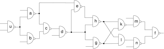
Figure 2: An example circuit.

Definition 5

For any $v\in\mathbb{D}_{u}$, the matching vector of $v$ with respect to $u$, denoted by $M_{u}(v)$, consists of all vertices $w\in\mathbb{V}$ such that $\{v,w\}$ is a double-vertex dominator of $u$. The order of vertices in $M_{u}(v)$ is defined as follows: If $\{v,w\}\in\mathbb{D}_{u}$ dominates $\{v,w^{\prime}\}\in\mathbb{D}_{u}$, then $w^{\prime}$ precedes $w$ in $M_{u}(v)$.

Lemma 10

For every $v\in\mathbb{D}_{u}$, there exist a unique matching vector $M_{u}(v)$.

Proof: The set of vertices which constitute $M_{u}(v)$ for a given $v\in\mathbb{D}_{u}$ is uniquely determined by the Definition 5. It remains to prove that the order of elements in $M_{u}(v)$ is unique.

By Definition 5, the vertices of $\mathbb{D}_{u}$ are ordered according to the dominator relation. Given any pair of double-vertex dominators of $u$, say $\{v,w\}$ and $\{v,w^{\prime}\}$, by Lemma 4, either $\{v,w\}$ dominates $w^{\prime}$, or $\{v,w^{\prime}\}$ dominates $w$. This implies that either $\{v,w\}$ dominates $\{v,w^{\prime}\}$, or $\{v,w^{\prime}\}$ dominates $\{v,w\}$. Thus, the order imposed by the dominator relation on the elements of $\mathbb{D}_{u}$ is total.

$\Box$

As an example, consider the circuit in Figure 2. The set of all double-vertex dominators of $u$ is: $\mathbb{D}_{u}=\{\{a,b\}$, $\{a,c\}$, $\{a,d\}$, $\{e,c\}$, $\{e,d\}$, $\{h,c\}$, $\{h,d\}$, $\{h,g\}$, $\{k,l\}$, $\{m,l\}$, $\{k,n\}$, $\{m,n\}\}$. Therefore, we have the following matching vectors with respect to $u$:

$$\begin{array}[]{l}M_{u}(a)=(b,c,d)\\ M_{u}(b)=(a)\\ M_{u}(c)=(a,e,h)\\ M_{u}(d)=(a,e,h)\\ M_{u}(e)=(c,d)\\ M_{u}(g)=(h)\\ M_{u}(h)=(c,d,g)\\ M_{u}(k)=(l,n)\\ M_{u}(l)=(k,m)\\ M_{u}(m)=(l,n)\\ M_{u}(n)=(k,m)\end{array}$$

Let $\mathbb{M}_{u}$ be the set of all matching vectors of all vertices in $\mathbb{D}_{u}$. The set $\mathbb{M}_{u}$ can be partitioned into a set of connected components which we call clusters.

Definition 6

A set of matching vectors $\mathbb{M}^{\prime}_{u}\subseteq\mathbb{M}_{u}$ is a cluster if:

1. $\forall M_{u}(v)\in\mathbb{M}^{\prime}_{u}$ and $\forall M_{u}(w)\in\mathbb{M}_{u}-\mathbb{M}^{\prime}_{u}$, $M_{u}(v)\cap M_{u}(w)=\emptyset$

2. $\mathbb{M}^{\prime}_{u}$ cannot be partitioned into two clusters satisfying (1).

In the example above, $\mathbb{M}_{u}$ can be partitioned into 4 clusters: $\{M_{u}(a),M_{u}(e),M_{u}(h)\}$, $\{M_{u}(b),M_{u}(c),M_{u}(d),M_{u}(g)\}$, $\{M_{u}(k),M_{u}(m)\}$, and $\{M_{u}(l),M_{u}(n)\}$.

Finally, we introduce a structure which will allow us to represent all clusters of $\mathbb{M}_{u}$ in linear space.

Definition 7

A vector $C(\mathbb{M}^{\prime}_{u})$ is the composition vector for a set of matching vectors $\mathbb{M}^{\prime}_{u}\subseteq\mathbb{M}_{u}$, if:

1. It contains each matching vector of $\mathbb{M}^{\prime}_{u}$ as a subvector,

2. It contains only matching vectors from $\mathbb{M}^{\prime}_{u}$,

3. It contains no duplicated vertices.

Theorem 7.1

For any two vertices $v,v^{\prime}\in\mathbb{D}_{u}$, it holds that either

1. $M_{u}(v)\cap M_{u}(v^{\prime})=$ suffix$(M_{u}(v))=$ prefix$(M_{u}(v^{\prime}))$, or

2. $M_{u}(v)\cap M_{u}(v^{\prime})=$ suffix$(M_{u}(v^{\prime}))=$ prefix$(M_{u}(v))$.

Proof: See Appendix A.

An obvious implication of the Theorem 7.1 is that, for any two matching vectors, there exists a composition vector. Furthermore if the two matching vectors have vertices in common, then the composition vector is unique (see Figure 3 for an illustration). It can also be shown that, for any set of matching vectors, there exists a composition vector.

In the example above, $C(M_{u}(a),M_{u}(e),M_{u}(h))=(b,c,d,g)$, $C(M_{u}(b),M_{u}(c),M_{u}(d),$ $M_{u}(g))=(a,e,h),C(M_{u}(k),M_{u}(m))=$ $(l,n)$, and $C(M_{u}(l),M_{u}(n))=(k,m)$. Note that the set of matching vectors of vertices of the first composition vector is equivalent to the second cluster, and vice verse. Similarly, the set of matching vectors of vertices of the third composition vector is equivalent to the fourth cluster, and vice verse. We call such clusters complimentary.

Definition 8

The cluster is complimentary to a cluster $\mathbb{M}^{\prime}_{u}\subseteq\mathbb{M}_{u}$, denoted by $\mathbb{\overline{M}}^{\prime}_{u}$, if the set of all matching vectors $M_{u}(v)$ of all $v\in C(\mathbb{M}^{\prime}_{u})$ constitute a cluster equivalent to $\mathbb{\overline{M}}^{\prime}_{u}$.

It is easy to show that if $\mathbb{\overline{M}}^{\prime}_{u}$ is complimentary to $\mathbb{M}^{\prime}_{u}$, then $\mathbb{M}^{\prime}_{u}$ is complimentary to $\mathbb{\overline{M}}^{\prime}_{u}$ as well. Each double-vertex dominator in $\mathbb{D}_{u}$ has one of its vertices in some cluster $\mathbb{M}^{\prime}_{u}\subseteq\mathbb{M}_{u}$ and another vertex in $\mathbb{\overline{M}}^{\prime}_{u}$. The following Lemma follows directly.

Lemma 11

The set $\mathbb{M}_{u}$ can be partitioned into pairs of complimentary clusters.

Figure 3: The relation between two overlapping matching vectors and their composition vector.

This brings us to the data structure for representing $\mathbb{D}_{u}$.

Definition 9

The set $\mathbb{D}_{u}$ of all double-vertex dominators of any $u\in\mathbb{V}$ can be represented by the dominator chain $\mathcal{D}(u)$ which is a vector of pairs of composition vectors of complimentary clusters of $\mathbb{M}_{u}$:

$$\mathcal{D}(u)=(\{C(\mathbb{M}^{1}_{u}),C(\mathbb{\overline{M}}^{1}_{u})\},\ldots,\{C(\mathbb{M}^{k}_{u}),C(\mathbb{\overline{M}}^{k}_{u})\}),$$

where $\mathbb{M}^{i}_{u}$ is the $i$th cluster of $\mathbb{M}_{u}$, for $i\in\{1,2,\ldots,k\}$. The order of clusters in $\mathcal{D}(u)$ is defined as follows: If $v$ is the first vertex of $C(\mathbb{M}^{i}_{u})$ and $w$ is the first vertex of $C(\mathbb{\overline{M}}^{i}_{u})$, then $\{v,w\}$ dominates every vertex in $C(\mathbb{M}^{j}_{u})$ and $C(\mathbb{\overline{M}}^{j}_{u})$ for all $i<j\leq k$. Each vertex $v$ which is contained in $\mathcal{D}(u)$ is associated with a pair $(v_{min},v_{max})$ representing of the first and the last vertex of $M_{u}(v)$.

For the circuit in Figure 2, the dominator chain for $u$ is

$$\mathcal{D}(u)=(\{(a,e,h),(b,c,d,g)\},\{(k,m),(l,n)\}),$$

$a$ is associated with $(b,d)$, $b$ is associated with $(a,a)$, etc.

8 Operations of Dominator Chains

One of the tasks for which dominator chains are used in this paper is to identify whether a given pair of vertices $\{v,w\}$ is a double-vertex dominator of some vertex $u\in\mathbb{V}$ or not. Assume that we have the dominator chain $\mathcal{D}(u)$ and that pairs $(v_{min},v_{max})$ consisting of the first and the last vertex of $M_{u}(v)$ are associated with each $v\in\mathbb{D}_{u}$. For each vertex $v^{\prime}\not\in\mathbb{D}_{u}$, we set $(v_{min},v_{max})=\emptyset$. Then, to determine whether $\{v,w\}$ is a double-vertex dominator of $u$, we first check whether $(v_{min},v_{max})$ and $(w_{min},w_{max})$ are empty. If they are, $\{v,w\}$ is not a dominator of $u$. Otherwise, we take $v_{min}$ and search for this vertex in $\mathcal{D}(u)$. The position of $v_{min}$ in $\mathcal{D}(u)$ gives us the starting point of $M_{u}(v)$. We need to traverse $M_{u}(v)$ until its last vertex, $v_{max}$, to determine whether $w\in M_{u}(v)$. If $w\in M_{u}(v)$, then $\{v,w\}$ is a dominator of $u$. Otherwise, $\{v,w\}$ is not a dominator of $u$. Such a procedure has a linear time complexity with respect to the size of $\mathcal{D}(u)$. However, ii can be further improved by indexing vertices of $\mathcal{D}(u)$ as follows.

We partition $\mathcal{D}(u)$ into two vectors $\mathcal{L}(u)$ (”left”) and $\mathcal{R}(u)$ (”right”). For each pair of composition vectors $\{C(\mathbb{M}^{i}_{u}),C(\mathbb{\overline{M}}^{i}_{u})\}$ in $\mathcal{D}(u)$, we put all vertices of one composition vector in $\mathcal{L}(u)$ and all vertices of another composition vector in $\mathcal{R}(u)$. It does not matter whether we put all $C(\mathbb{M}^{i}_{u})$ in $\mathcal{L}(u)$ and all $C(\mathbb{\overline{M}}^{i}_{u})$ in $\mathcal{R}(u)$, or vice verse. However, once we make a choice for the first pair of composition vectors in $\mathcal{D}(u)$, this choice should be followed for all pairs in $\mathcal{D}(u)$. It is also possible to make $\mathcal{L}(u)$ and $\mathcal{R}(u)$ unique by imposing the topological order on vertices of the circuit graph. In this case, we put $C(\mathbb{M}^{i}_{u})$ in $\mathcal{L}(u)$ if the first vertex of $C(\mathbb{M}^{i}_{u})$ precedes the first vertex of $C(\mathbb{\overline{M}}^{i}_{u})$. Otherwise, we put $C(\mathbb{M}^{i}_{u})$ in $\mathcal{R}(u)$.

For the circuit in Figure 2, the dominator chain can be partitioned as follows:

$$\begin{array}[]{l}\mathcal{L}(u)=(a,e,h,k,m),\\ \mathcal{R}(u)=(b,c,d,g,l,n).\end{array}$$

To make possible a constant time look-up for dominators, three parameters are assigned to vertices:

• For all $v\in\mathbb{D}_{u}$ we assign $flag(v)\in\{$ left,right $\}$, which distinguishes whether $v$ belongs to $\mathcal{L}(u)$ or $\mathcal{R}(u)$.

• For all $v\in\mathcal{L}(u)(\mathcal{R}(u))$, we assign $index(v)$ which indicates the position of $v$ in $\mathcal{L}(u)(\mathcal{R}(u))$.

• Instead of associating with each $v\in\mathbb{D}_{u}$ a pair of vertices $(v_{min},v_{max})$, we associating with each $v$ a pair of indexes $(min,max)$, where $min(v)=index(v_{min})$, $max(v)=index(v_{max})$.

In the example above, $flag(a)=$ left, $flag(b)=$ right, $index(b)=1$, $index(c)=2$, $(min(b),max(b))=(1,1)$, $(min(c),max(c))=(1,3)$, etc.

Now we can check whether $\{v,w\}$ dominates $u$ as follows:

1. Check if $flag(v)\not=flag(w)$. If yes, go to step 2. Otherwise, $\{v,w\}\not\in\mathbb{D}_{u}$.

2. Check if $min(v)\leq index(w)\leq max(v)$. If yes, $\{v,w\}\in\mathbb{D}_{u}$. Otherwise, $\{v,w\}\not\in\mathbb{D}_{u}$.

9 An Algorithm for Finding Dominators

The algorithm presented in this section takes as its input a circuit graph $G=(\mathbb{V},\mathbb{E},root)$ and a vertex $u\in\mathbb{V}$. It returns the dominator chain $\mathcal{D}(u)$. The pseudo-code of the algorithm is shown in Figure 4.

In order to construct $\mathcal{D}(u)$, the following steps are followed:

1. Find all single-vertex dominators of $u$.

2. Set $\mathcal{D}(u)=\emptyset$ and $v=u$.

3. Construct the dominator chain $\mathcal{D}(v)$ for $v$ assuming that $idom(v)$ is the sink and append it to the end of $\mathcal{D}(u)$.

4. Set $v=idom(v)$ and repeat Step 3 until $v\neq root$.

To simplify the description of the algorithm, we assume that there are no single-vertex dominators of $u$ with respect to $root$, i.e. we focus on the Steps 3 and 4.

algorithm $\textsc{DominatorChain}(\mathbb{V},\mathbb{E},root,u)$
input: $\mathbb{V}$ is a set of vertices, $\mathbb{E}\subseteq\mathbb{V}\times\mathbb{V},root\in\mathbb{V},u\in\mathbb{V}$.
	Construct a path $P_{1}\subseteq V$ from $u$ to $root$;
	Construct a path $P_{2}\subseteq V$ from $u$ to $root$ such that $P_{2}\cap P_{1}=\{u,root\}$;
	Construct a path $P_{3}\subseteq V$ from $u$ to $root$ such that $P_{3}\cap(P_{1}\cup P_{2})=\{u,root\}$;
	if $P_{3}$ is constructed then
		return $\mathcal{D}(u)=\emptyset$;
	for each $v\in\mathbb{V}$ do
		Set marked(v) = 0;
	end
	$\textsc{AssignMinMax}(P_{1},P_{2})$;
	for each $v\in\mathbb{V}$ do
		Set marked(v) = 0;
	end
	$\textsc{AssignMinMax}(P_{2},P_{1})$;
	$\mathcal{L}(u)=\textsc{ConstructVector}(P_{1},P_{2})$;
	$\mathcal{R}(u)=\textsc{ConstructVector}(P_{2},P_{1})$;
	$\textsc{ConvertMinMax}(\mathcal{L}(u),P_{2})$;
	$\textsc{ConvertMinMax}(\mathcal{R}(u),P_{1})$;
	return $\textsc{ConstructD\_u}(\mathcal{L}(u),\mathcal{R}(u))$;
end

Figure 4: Pseudo-code of the presented algorithm for finding double-vertex dominators of a vertex $u$.

The presented algorithm exploits the following property of disjoint paths. Recall that we call two paths disjoint if the intersection of sets of their non-terminal vertices is empty.

Lemma 12

If there are two disjoint paths from $u$ to $root$, $P_{1}$ and $P_{2}$, then, for any double-vertex dominator $\{v,w\}$ of $u$, it holds that $v\in P_{1}$ and $w\in P_{2}$.

Proof: By Definition 2, at least one vertex of the double-vertex dominator $\{v,w\}$ should be present in any path from $u$ to $root$. Since $P_{1}$ and $P_{2}$ are disjoint, none of their vertices belong to both paths except $u$ and $root$. Vertices $u$ and $root$ are single vertex dominators of $u$, thus they do not belong to $\mathbb{D}_{u}$. Therefore, one vertex of the pair $\{v,w\}$ should belong to $P_{1}$ and another one to $P_{2}$.

$\Box$

It directly follows from the Lemma 12 that if there exists a third path from $u$ to $root$ which is disjoint with both $P_{1}$ and $P_{2}$, then $u$ has no double-vertex dominators. We use this property to bound the search space for double-vertex dominators.

algorithm $\textsc{AssignMinMax}(P_{1},P_{2})$
input: $P_{1}=(v_{1}=u,v_{2},v_{3},\ldots,v_{|P_{1}|}=root)$,
$P_{2}=(w_{1}=u,w_{2},w_{3},\ldots,w_{|P_{2}|}=root)$.
	$reached\_P_{1}=0$;
	$reached\_P_{2}=1$;
	$new\_reached\_P_{1}=reached\_P_{1}$;
	$new\_reached\_P_{2}=reached\_P_{2}$;
	$last\_prime=0$;
	for each $i$ from 1 to $|P_{1}|-1$ do
		if $reached\_P_{1}>i$ then
			/*By setting $min(v_{i})=|P_{2}|$ we remove $v_{i}$ from*/
			/*the list of potential candidates into dominators*/
			$min(v_{i})=|P_{2}|$;
			$prime(v_{i})=last\_prime$;
		else
			$min(v_{i})=reached\_P_{2}$;
			$prime(v_{last\_prime})=i$;
			$last\_prime=i$;
		$\textsc{FindReachable}(v_{i},P_{1},P_{2})$;
		if $reached\_P_{1}<new\_reached\_P_{1}$ then
		$reached\_P_{1}=new\_reached\_P_{1}$
		if $reached\_P_{2}>=new\_reached\_P_{2}$ then break
		for each $j$ from $reached\_P_{2}$ to $new\_reached\_P_{2}-1$ do
			$max(w_{j})=i$;
		end
		$reached\_P_{2}=new\_reached\_P_{2}$;
	end
	$prime(v_{last\_prime})=|P_{1}|$;
end

Figure 5: Pseudo-code of the procedure AssignMinMax.

We search for three disjoint paths from $u$ to $root$ using a modified version of the max-flow algorithm which operates on vertex rather than edge capacities [24]. The max-flow algorithm attempts to construct three augmenting paths with $u$ as the source and $root$ as the sink. Each vertex is assigned a unit capacity. The net flow through each vertex should be either one or zero. Therefore, the resulting augmenting paths are mutually disjoint by construction.

If the algorithm succeeds to find three disjoint paths, then by Lemma 12, $\mathbb{D}_{u}=\emptyset$. If only two disjoint paths are found, then we conclude that vertices on these paths are potential candidates for $\mathbb{D}_{u}$. The Lemma below helps us to distinguish which of them can belong to $\mathbb{D}_{u}$ and which are not.

Lemma 13

Let $P_{1}=(v_{1}=u,v_{2},v_{3},\ldots,v_{|P_{1}|=root})$ and $P_{2}$ be two disjoint paths from $u$ to $root$. If there exists a path $P_{3}$ which starts at some vertex $v_{i}\in P_{1}$, ends at some vertex $v_{j}\in P_{1}$, $i,j\in\{1,2,\ldots,|P_{1}|\}$, and has not other common vertices with neither $P_{1}$ nor $P_{2}$, then $v_{k}\not\in\mathbb{D}_{u}$ for all $v_{k}\in P_{1}$ such that $i<k<j$.

Proof: The path $P_{1}$ can be seen as concatenation of three paths $P_{1}=P_{4}P_{5}P_{6}$ where $P_{4}$ is a prefix of $P_{1}$ having $v_{i}$ as its last vertex, $P_{6}$ is a suffix of $P_{1}$ having $v_{j}$ as its first vertex, and $P_{5}$ is the middle part of $P_{1}$ containing all vertices from $v_{i}$ to $v_{j}$. Denote by $P_{7}$ a path $P_{7}=P_{4}P_{3}P_{6}$.

Consider some vertex $v_{k}\in P_{5}$. Since $v_{k}\in P_{5}$ and $v_{k}$ cannot appear twice in $P_{1}$, $v_{k}\not\in P_{4}$ and $v_{k}\not\in P_{6}$. Since $P_{1}$ and $P_{3}$ have no common vertices except $v_{i}$ and $v_{j}$, we can conclude that $v_{k}\not\in P_{3}$. This implies that $v_{k}\not\in P_{7}$, and also that $v_{k}\not\in P_{2}$, because $P_{1}$ and $P_{2}$ are disjoint. Since paths $P_{2}$ and $P_{7}$ are two disjoint paths from $u$ to $root$ and $v_{k}$ does not belong to any of them, by Lemma 12, $v_{k}\not\in\mathbb{D}_{u}$.

$\Box$

We call a vertex $v\in\mathbb{V}$ prime if any path from an ancestor of $v$ to a descendant of $v$ contains $v$. By the Lemma 13, any pair of prime vertices $\{v,w\}$ such that $v\in P_{1}$ and $w\in P_{2}$, and $P_{1}$ and $P_{2}$ are disjoint, can potentially be a double-vertex dominator of $u$. The next Lemma put additional restrictions of pairs of vertices that can belong to $\mathbb{D}_{u}$.

Lemma 14

Let $P_{1}=(v_{1}=u,v_{2},v_{3},\ldots,v_{|P_{1}|}=root)$ and $P_{2}=(w_{1}=u,w_{2},w_{3},\ldots,w_{|P_{2}|}=root)$ be two disjoint paths from $u$ to $root$. If there exists a path $P_{3}$ which starts at some vertex $v_{i}\in P_{1}$, ends at some vertex $w_{j}\in P_{2}$, and has not other common vertices with $P_{1}$ and $P_{2}$, then all pairs of vertices $\{v_{k},w_{l}\}$ such that $i<k\leq|P_{1}|$ and $1\geq l<j$ are not in $\mathbb{D}_{u}$.

Proof: The path $P_{1}$ can be seen as a concatenation of two paths $P_{1}=P_{4}P_{5}$ where $P_{4}=(v_{1},\ldots,v_{i})$ and $P_{6}=(v_{i},\ldots,v_{|P_{1}|})$. Similarly, the path $P_{2}$ can be seen as a concatenation of two paths $P_{2}=P_{6}P_{7}$ where $P_{6}=(w_{1},\ldots,w_{j})$ and $P_{7}=(w_{i},\ldots,w_{|P_{2}|})$. Denote by $P_{8}$ a path $P_{8}=P_{4}P_{3}P_{7}$.

Since $P_{1}$ and $P_{3}$ have no common vertices except $v_{i}$, we can conclude that, for any $i<k\leq|P_{1}|$, $v_{k}\not\in P_{3}$. Similarly, for any $1\geq l<j$, $w_{l}\ \not\in P_{3}$ because $P_{2}$ and $P_{3}$ have no common vertices except $w_{j}$.

Since, for any $i<k\leq|P_{1}|$, $v_{k}\not\in P_{3}$ and $v_{k}$ cannot appear twice in $P_{1}$, $v_{k}\not\in P_{4}$. Also, for any $1\geq l<j$, $w_{l}\ \not\in P_{4}$ because $P_{1}$ is disjoint with $P_{2}$.

Similarly, since for any $1\geq l<j$, $w_{l}\ \not\in P_{6}$ and $w_{l}$ cannot appear twice in $P_{2}$, $w_{l}\ \not\in P_{7}$. Also, for any $i<k\leq|P_{1}|$, $v_{k}\not\in P_{7}$ because $P_{1}$ is disjoint with $P_{2}$.

It follows from above that, for any $i<k\leq|P_{1}|$ and $1\geq l<j$, $v_{k},w_{l}\not\in P_{8}$. Since $P_{8}$ is a path from $u$ to $root$, by the Definition 2 that $\{v_{k},w_{l}\}\not\in\mathbb{D}_{u}$.

$\Box$

algorithm $\textsc{FindReachable}(x,P_{1},P_{2})$
input: $x\in\mathbb{V}$, $P_{1}=(v_{1}=u,v_{2},v_{3},\ldots,v_{|P_{1}|}=root)$,
$P_{2}=(w_{1}=u,w_{2},w_{3},\ldots,w_{|P_{2}|}=root)$.
	Let $P_{1}=(v_{1}=u,v_{2},v_{3},\ldots,v_{|P_{1}|}=root)$;
	Let $P_{2}=(w_{1}=u,w_{2},w_{3},\ldots,w_{|P_{2}|}=root)$;
	for each $y\in$ TransFanout$(x)$ do
		if $marked(y)=1$ then break
		$marked(y)=1$;
		if $y=root$ then return $(|P_{1}|,|P_{2}|)$;
		if $y=v_{i}$ then
			if $i>new\_reached\_P_{1}$ then $new\_reached\_P_{1}=i$;
			break
		if $(y=w_{j})$ then
			if $n>new\_reached\_P_{2}$ then $new\_reached\_P_{2}=j$;
			break
	end
end

Figure 6: Pseudo-code of the procedure FindReachable.

We use fields $max$ and $min$ of vertices of $P_{1}$ and $P_{2}$ to keep track of potential double-vertex dominators during the execution of the algorithm. If the field $max(v_{k})$ of some $v_{k}\in P_{1}$ is assigned to $max(v_{k})=i$, that means that we have identified that $\{v_{k},w_{j}\}\not\in\mathbb{D}_{u}$ for all $w_{j}\in P_{2}$ such that $j>i$. Similarly, if the field $max(v_{k})$ of $v_{k}\in P_{1}$ is assigned to $max(v_{k})=i$, then we have identified that $\{v_{k},w_{j}\}\not\in\mathbb{D}_{u}$ for all $w_{j}\in P_{2}$ such that $j<i$.

The rules for assigning $max$ and $min$ fields follow from the Lemma 14. If there exist a path $P_{3}=(v_{i},\ldots,w_{j})$, $v_{i}\in P_{1}$, $w_{j}\in P_{2}$, disjoint with $P_{1}$ and $P_{2}$, then $max(w_{k})\leq i$ for all $k$ such that $1<k\leq j-1$ and $min(v_{l})\geq j$ for all $l$ such that $k+1\geq l<|P_{1}|$. Note that we write an inequality sign because there might be another path $P_{4}=(v_{m},\ldots,w_{n})$ disjoint with $P_{1}$ and $P_{2}$ such that $m<i$ and $n>j$. In this case, $max(w_{k})\leq m$ and $min(v_{l})\geq n$. All paths disjoint with $P_{1}$ and $P_{2}$ should be considered to determine which indexes should be assigned to $max$ and $min$ fields. The following property summarizes the rules for assigning $max$ and $min$ fields.

Property 1

Let $P_{1}$ and $P_{2}$ be two disjoint paths from $u$ to $root$. Let $P_{3}=(v_{i},\ldots,w_{j})$, $v_{i}\in P_{1}$, $w_{j}\in P_{2}$, be a path disjoint with $P_{1}$ and $P_{2}$. Then:

• $max(v_{k})=i$, $\forall w_{k}\in P_{2}$ such that $k<j$, where $i$ is the minimal index of a vertex of $P_{1}$ for which the path $P_{3}$ exists.

• $max(v_{k})=j$, $\forall v_{k}\in P_{1}$ such that $k>i$, where $j$ be the maximal index of a vertex of $P_{2}$ for which the path $P_{3}$ exists.

algorithm $\textsc{ConstructVector}(P_{1},P_{2})$
input: $P_{1}=(v_{1}=u,v_{2},v_{3},\ldots,v_{|P_{1}|}=root)$,
$P_{2}=(w_{1}=u,w_{2},w_{3},\ldots,w_{|P_{2}|}=root)$.
	$index\_count=1$;
	$\mathcal{V}(u)=\emptyset$;
	for each $i$ from 2 to $|P_{1}|-1$ do
		$min=min(v_{i})$;
		$max=max(v_{i})$;
		if $min=|P_{2}|$ then break
		if $min(w_{min})=|P_{1}|$ then
			/*min field is set to the index of the closest*/
			/*prime descendant of $w_{min}$ in $P_{2}$ */
			$min(v_{i})=prime(w_{prime(w_{min})})$;
		if $min(w_{max})=|P_{1}|$ then
			/*max field is set to the index of the closest*/
			/*prime ancestor of $w_{max}$ in $P_{2}$*/
			$max(v_{i})=prime(w_{max})$;
		if $min(v_{i})<=max(v_{i})$ then
			Append $v_{i}$ to the end of vector $\mathcal{V}(u)$;
			$index(v_{i})=index\_count$;
			$index\_count=index\_count+1$;
	end
	return $\mathcal{V}(u)$;
end

Figure 7: Pseudo-code of the procedure ConstructVector.

algorithm $\textsc{ConvertMinMax}(\mathcal{V}(u),P_{2})$
input: $\mathcal{V}(u)\subseteq V$, $P_{2}=(w_{1}=u,w_{2},w_{3},\ldots,w_{|P_{2}|}=root)$.
	for all $v\in\mathcal{V}(u)$ do
		$min(v)=index(w_{min(v)})$;
		$max(v)=index(w_{max(v)})$;
	end
end

Figure 8: Pseudo-code of the procedure ConvertMinMax.

The procedure $\textsc{AssignMinMax}(P_{1},P_{2})$, shown in Figure 5, allocates $max(v_{i})$ field for all vertices $v_{i}\in P_{1}$ and $min(w_{j})$ field for all vertices $w_{j}\in P_{2}$. This procedure also checks whether vertices of $P_{1}$ are prime or not. If $v_{i}\in P_{1}$ is not a prime, then its field $prime(v_{i})$ is set to the index of the closest prime ancestor of $v_{i}$ in $P_{1}$. If $v_{i}\in P_{1}$ is a prime, then its field $prime(v_{i})$ is set to the index of the closest prime descendant of $v_{i}$ in $P_{1}$.

The main loop of the procedure $\textsc{AssignMinMax}(P_{1},P_{2})$ iterates through all vertices $v_{i}$ of $P_{1}$ from the source to the sink of $P_{1}$. For every $i$, in the beginning of the main loop, the variable $reached\_P_{1}$ contains the maximum index of a vertex of $P_{1}$ that can be reached from an ancestor of $v_{i}$ in $P_{1}$ by a path disjoint with $P_{1}$ and $P_{2}$. Similarly, the variable $reached\_P_{2}$ contains the maximum index of a vertex of $P_{2}$ that can be reached from an ancestor of $v_{i}$ in $P_{1}$ by a path disjoint with $P_{1}$ and $P_{2}$.

In the main loop, first we check whether $v_{i}$ is prime or not. If $reached\_P_{1}>i$, it means that there exists a path $P_{3}$ from an ancestor of $v_{i}$ in $P_{1}$ to a descendant of $v_{i}$ in $P_{1}$ which is disjoint with $P_{1}$ and $P_{2}$. Thus by Lemma 13 $v_{i}$ is not prime. If $reached\_P_{1}\leq i$ then no such path exists and $v_{i}$ can be declared prime. According to the Property 1b $min(v_{i})$ is set to $reached\_P_{2}$.

The procedure FindReachable, described later in this section, is used to update a pair of global variables $new\_reached\_P_{1}$ and $new\_reached\_P_{2}$. The values $new\_reached\_P_{1}$ represents the maximum index of a vertex of $P_{1}$ that can be reached from $v_{i}$ or any ancestor of $v_{i}$ in $P_{1}$ by a path disjoint with $P_{1}$ and $P_{2}$. Since $v_{i}$ is an ancestor of $v_{i+1}$, $new\_reached\_P_{1}$ represents the value of $reached\_P_{1}$ for the next iteration of main loop. Similarly, the value $new\_reached\_P_{2}$ represents the maximum index of a vertex of $P_{2}$ that can be reached from $v_{i}$ or any of its ancestors in $P_{1}$ by a path with is disjoint with $P_{1}$ and $P_{2}$. Thus, $new\_reached\_P_{2}$ represents the value of $reached\_P_{2}$ for the next iteration of the main loop.

If $new\_reached\_P_{2}>reached\_P_{2}$, this means that, for every vertex $w_{j}\in P_{2}$ in the range $(w_{reached\_P_{2}},\ldots,w_{new\_reached\_P_{2}-1})$, $i$ is the minimum index of a vertex in $P_{1}$ for which there exists a to a descendant of $w_{j}$ in $P_{2}$ which is disjoint with $P_{1}$ and $P_{2}$. According to the Property 1a $max(w_{j})$ is set to $i$.

The procedure $\textsc{FindReachable}(x,P_{1},P_{2})$ sets $marked(y)=1$ for all vertices $y$ which are reachable by path which is disjoint with $P_{1}$ and $P_{2}$ from a given vertex $x$ and updates global variables $new\_reached\_P_{1}$ and $new\_reached\_P_{2}$. The marking is performed by a depth-first search. Any path disjoint with $P_{1}$ and $P_{2}$ which contains $y\not\in P_{1}\cap P_{2}$ can be extended to any of the vertices in the fanout of $y$. Such an extended path is disjoint with $P_{1}$ and $P_{2}$ as well. So, all vertices in the fanout of $y$ are reachable by paths disjoint with $P_{1}$ and $P_{2}$, and therefore they are marked. FindReachable is called for all newly marked vertices which do not belong to neither $P_{1}$ or $P_{2}$.

The maximum index of each marked vertex in a path $P_{1}$ ($P_{2}$) is stored in the global variable $new\_reached\_P_{1}$ ($new\_reached\_P_{2}$). This variable represents the maximum index of a vertex of $P_{1}$ ($P_{2}$) that can be reached by a disjoint with $P_{1}$ and $P_{2}$ path from one of the vertices $x$ for which $\textsc{FindReachable}(x,P_{1},P_{2})$ was initially called.

The following theorem states that once all fields $min$ and $max$ are set by AssignMin $\textsc{Max}(P_{1},P_{2})$ and $\textsc{AssignMinMax}(P_{2},P_{1})$, all remaining potential candidates to double-vertex dominators are indeed double-vertex dominators.

Theorem 9.1

Let $P_{1}$ and $P_{2}$ be two disjoint paths from $u$ to $root$. If vertices $v_{i}\in P_{1}$ and $w_{j}\in P_{2}$ are prime, $max(w_{j})\geq i$, and $min(w_{j})\leq i$, then $\{v_{i},w_{j}\}$ is a double-vertex dominator of $u$.

Proof: See Appendix B.

algorithm $\textsc{ConstructD\_u}(\mathcal{L}(u),\mathcal{R}(u))$
input: $\mathcal{L}(u)=(v_{1},v_{2},\ldots,v_{|\mathcal{L}(u)|})$, $\mathcal{L}(u)=(w_{1},w_{2},\ldots,w_{|\mathcal{R}(u)|})$.
	$begin_{L}=1$; $begin_{R}=1$;
	$end_{L}=1$; $end_{R}=1$;
	$i=1$;
	$\mathcal{D}(u)=\emptyset$;
	while $end_{L}\neq|\mathcal{L}(u)|$ do
		while 1 do
			$end_{Rnew}=max(v_{end_{L}})$;
			if $end_{Rnew}=end_{R}$ then break
			$end_{R}=end_{Rnew}$;
			$end_{Lnew}=max(w_{end_{R}})$;
			if $end_{Lnew}=end_{L}$ then break
			$end_{L}=end_{Lnew}$;
		end
		Set $C(\mathbb{M}^{i}_{u})=\{v_{begin_{L}},\ldots,v_{end_{L}}\}$; /*$C(\mathbb{M}^{i}_{u})\subseteq\mathcal{L}(u)$*/
		Set $C(\mathbb{\overline{M}}^{i}_{u})=\{w_{begin_{R}},\ldots,w_{end_{R}}\}$; /*$C(\mathbb{\overline{M}}^{i}_{u})\subseteq\mathcal{R}(u)$*/
		Append $\{C(\mathbb{M}^{i}_{u}),C(\mathbb{\overline{M}}^{i}_{u})\}$ to $\mathcal{D}(u)$;
		$i=i+1$;
		$begin_{L}=end_{L}$;
		$begin_{R}=end_{R}$;
	end

Figure 9: Pseudo-code of the procedure ConstructD_u.

The procedure $\textsc{ConstructVector}(P_{1},P_{2})$ returns the vector $\mathcal{V}(u)$, which is either $\mathcal{L}(u)$ or $\mathcal{R}(u)$. The vector $\mathcal{V}(u)$ consists of a subset of vertices of $P_{1}$. According to the Theorem 9.1, a vertex $v_{i}$ belongs to $\mathcal{V}(u)$ if there exists at least one prime vertex in $P_{2}$ which is in the range between $min(v_{i})$ and $max(v_{i})$. First, we check whether $min(v_{i})$ and $max(v_{i})$ contain indexes of prime vertices. If not, then they are updated as follows. The field $min(v_{i})$ is set to the minimum index of prime vertices $w_{j}$ in $P_{2}$ satisfying $j>min(v_{i})$. Similarly, the $max(v_{i})$ is set to the maximum index of prime vertices $w_{j}$ in $P_{2}$ satisfying $j<max(v_{i})$. Finally, if $min(v_{i})\leq max(v_{i})$, then we can conclude that $\{v_{i},w_{min(v_{i})}\}$ and $\{v_{i},w_{max(v_{i})}\}$ are double-vertex dominators of $u$ and append $v_{i}$ at the end of $\mathcal{V}(u)$. At this point, the position of $v_{i}$ in $\mathcal{V}(u)$ is known. Therefore, we set the index of $v_{i}$ to $index\_count$. However, indexes of vertices $min(v_{i})$ and $max(v_{i})$ in the complimentary to $\mathcal{V}(u)$ vector of the dominator chain are not known yet. These indexes are assigned later by the procedure $\textsc{ConvertMinMax}(\mathcal{V}(u),P_{2})$.

Finally, the dominator chain $\mathcal{D}(u)$ is constructed by the procedure ConstructD_u $(\mathcal{L}(u),\mathcal{R}(u))$. This procedure is optional, since for some applications it is sufficient to find $\mathcal{L}(u)$ and $\mathcal{R}(u)$ along with $min(v)$, $max(v)$ for all $v\in\mathbb{D}_{u}$.

The procedures $\textsc{ConstructVector}(P_{1},P_{2})$, Convert $\textsc{MinMax}(\mathcal{V}(u),P_{2})$ and $\textsc{ConstructD\_u}(\mathcal{L}(u),\mathcal{R}(u))$ have linear complexity with respect to $|P_{1}|$, $|\mathcal{V}(u)|$, and $|\mathcal{L}(u)+\mathcal{R}(u)|$ respectively. The procedure $\textsc{FindReachable}(x,P_{1},P_{2})$ is called at most once for every vertex during the call of $\textsc{AssignMinMax}(P_{2},P_{1})$. Each call of FindRe- $\textsc{achable}(x,P_{1},P_{2})$ iterates through all vertices in the fanout of $x$, thus AssignMin $\textsc{Max}(P_{2},P_{1})$ has linear time complexity with respect to the number of edges $\mathbb{E}$ in the input graph.

Since all procedures of $\textsc{DominatorChain}(\mathbb{V},\mathbb{E},root,u)$ have linear complexity with respect to $|\mathbb{E}|$, the presented algorithm has the complexity $O(|\mathbb{E}|)$. Its execution time is dominated by the execution time of the procedures $\textsc{AssignMinMax}(P_{1},P_{2})$ and $\textsc{AssignMinMax}(P_{2},P_{1})$. Therefore, the actual execution time of the presented algorithm is proportional to $2|\mathbb{E}^{\prime}|$, where $\mathbb{E}^{\prime}\subseteq\mathbb{E}$ is the set of edges in the transitive fanout of $u$.

			2-input	All	All	Useful	Runtime, sec
Name	Inputs	Outputs	AND gates	1-doms	2-doms	2-doms	[21]	[8]	presented
clma	94	115	24277	948	9819	2867	88.52	0.41	0.34
clmb	415	402	23906	361	8638	2356	98.09	0.53	0.45
mult32	64	96	10594	1150	27507	16442	885.62	2.98	1.45
apex2	38	3	8755	853	1551	890	162.16	0.23	0.16
too_large	38	3	8746	971	2238	1467	136.02	0.22	0.14
misex3	14	14	8155	59	2657	1224	29.83	0.17	0.12
seq	41	35	7462	1796	27631	13879	9.62	0.25	0.16
cordic_latches	318	294	6212	7313	31714	12214	4.27	0.36	0.28
bigkey	452	421	5661	2016	8822	2421	4.16	0.33	0.23
s15850s	553	627	5389	27210	170189	31245	25.23	0.81	0.41
alu4	14	8	5285	134	706	449	28.06	0.08	0.08
des	256	245	4733	3361	9231	2349	2.56	0.25	0.17
s15850	611	684	4172	34564	74941	16975	18.52	0.77	0.45
apex5	114	88	3781	800	21728	8107	0.95	0.17	0.12
key	452	421	3537	1348	7717	2740	2.17	0.28	0.19
i8	133	81	3444	2068	8121	3296	0.83	0.12	0.09
ex1010	10	10	3278	0	545	92	11.33	0.14	0.14
dsip	452	421	2975	2245	6586	2059	1.75	0.23	0.2
i10	257	224	2935	6446	81707	30608	4.95	0.47	0.2
apex4	9	19	2905	0	841	165	8.7	0.12	0.09
s13207s	483	574	2590	3179	13365	6673	2.28	0.22	0.16
apex3	54	50	2419	1723	34386	29957	6.66	0.2	0.11
C6288	32	32	2370	480	5743	3366	1.67	0.27	0.2
C7552	207	108	2282	4604	87027	14728	19.12	0.31	0.11
k2	45	45	2236	1827	16400	11693	5.42	0.17	0.08
total for 214				177577	3777809	935309	1637.47	30.77	17.27

Table 1: Benchmark results for IWLS’02 benchmark set.

10 Experimental Results

In this section, we compare the performance of the presented algorithm to the algorithm for finding double-vertex dominators from [8] and to the algorithm finding multiple-vertex dominators from [21]. The algorithm [21] can compute all $k$-vertex dominators of a given vertex for any $k$. In our experiment, we set $k$ to 2.

We have applied the three algorithms to 214 combinational benchmarks from the IWLS’02 benchmark set. Table 1 shows the results for 25 largest of these benchmarks. Columns 1, 2, 3 and 4 show the name of the benchmark, the number of primary inputs, the number of primary outputs, and the number of 2-input AND gates in the benchmark, respectively. In the last row of the Table 1, the $total$ is computed for all 214 benchmarks.

In our experiments, we treated every primary output of a multiple-output circuit as a separate function. Circuits for every primary output were extracted from the original multiple-output circuit. For each resulting single-output circuit, all dominators were computed for every primary input with respect to the primary output. The numbers shown in Columns 5, 6 and 7 give the total number of dominators for all single output circuits of the corresponding benchmark. The same dominator of several inputs was counted as one dominator.

In Column 5, we show the total number of single-vertex dominators (except trivial dominators which are primary inputs and the primary output), computed using the Lengauer and Tarjan’s algorithm [1].

Column 6 shows the total number of double-vertex dominators computed by the presented algorithm, the algorithm  [8] and the algorithm [21]. All three algorithms found all double vertex-dominators, therefore they produce the same result. For most applications, useful dominators are those which dominate more vertices then the size of the dominator itself. Thus, in Column 7, we also show the number of all ”useful” double-vertex which dominate at least three primary inputs.

Columns 8, 9, and 10 show the runtime of three algorithms, in seconds. The time was measured using the Unix command $time$ (user time). The experiments were performed on a PC with a 1600 MHz AMD Turion64 CPU and 1024 MByte main memory.

From Table 1 we can see that the presented algorithm and the algorithm [8] substantially outperform the algorithm [21], delivering, on average, an order of magnitude runtime reduction. This is not surprising since they are specifically designed for double-vertex dominators. We can also see that the presented algorithm consistently outperforms the algorithm [8] on all benchmarks presented in Table 1.

In our implementation, the original benchmark circuits were converted to an And-Inverter graph which consists of 2-input AND gates and Inverters [25]. In such a graph, the majority of single vertex dominators have the corresponding trivial double-vertex dominator (a pair of vertices feeding the single-vertex dominator). The number of such trivial double-vertex dominators can be roughly overapproximated to be equal to the number of single-vertex dominators. Trivial double vertex dominators are usually less useful than the corresponding single-vertex dominator. So, the numbers in Column 7 should be reduced by the numbers in Column 5 to get a better picture of the number of useful dominators.

Some rare circuits have less double-vertex dominators than single-vertex dominators. Recall that our definition of multiple-vertex dominators excludes redundancies. Therefore, in the extreme case of a tree-like circuit with $n$ vertices the number of single-vertex dominators is $n$ while the number of double-vertex dominators is 0.

11 Conclusion

This paper presents supporting theory and algorithms for finding double-vertex dominators in directed acyclic graphs. Our results provide an efficient systematic way of partitioning a graph along the reconverging points of its signal flow. They might be useful in a number of CAD applications, including signal probability computation, switching activity estimation and cut point identification. For example, in the method presented in [6], cut-points are used to progressively abstract a functional representation by quantification. Our dominator-based approach can complement this method by providing a systematic way of identifying and selecting good cut-points for the abstraction.

Our results might also find potential applications beyond CAD borders. In general, any technique which use dominators in a directed acyclic graph might benefit from this work.

Appendix

A. Proof of the Theorem 7.1: Let $n$ denote the number of vertices common for $M_{u}(v)$ and $M_{u}(v^{\prime})$. If $n=0$, then the Theorem 7.1 holds trivially with vector $M_{u}(v)\cap M_{u}(w)$ being empty.

Assume that $n>0$. We divide the prove into two parts. In the first part, we prove that all $n$ common vertices should be in a suffix of one vector, and in a prefix of the other one. In the second part, we prove that the order of common vertices is the same in both vectors.

Part 1: By assumption, there exists a common vertex, say $w\in\mathbb{V}$, which belong to both $M_{u}(v)$ and $M_{u}(v^{\prime})$. This implies that there exist dominators $\{v,w\}\in\mathbb{D}_{u}$ and $\{v^{\prime},w\}\in\mathbb{D}_{u}$. According to the Lemma 4, either $\{v,w\}$ dominates $v^{\prime}$ or $\{v^{\prime},w\}$ dominates $v$. This also means that either $\{v,w\}$ dominates $\{v^{\prime},w\}$, or $\{v^{\prime},w\}$ dominates $\{v,w\}$. Without any loss of generality, assume that $\{v,w\}$ dominates $\{v^{\prime},w\}$.

First, we prove that a prefix of $M_{u}(v)$ whose last element is $w$ is always a subvector of $M_{u}(v^{\prime})$ and a suffix of $M_{u}(v^{\prime})$ whose first element is $w$ is always a subvector of $M_{u}(v)$.

Due to the antisymmetry of the dominator relation, $\{v^{\prime},w\}$ does not dominate $\{v,w\}$. Since $w$ is dominated by $\{v^{\prime},w\}$, thus $v$ is not dominated by $\{v^{\prime},w\}$.

By the Definition 5, $\{v,w\}$ dominates $\{v,w^{\prime}\}$ for every vertex $w^{\prime}$ preceding $w$ in $M_{u}(v)$. Due to the antisymmetry of dominator relation, $\{v,w^{\prime}\}$ does not dominate $\{v,w\}$. Since $v$ is dominated by $\{v,w^{\prime}\}$, thus $w$ is not dominated by $\{v,w^{\prime}\}$.

To summarize, we derived that there are dominators $\{v^{\prime},w\}\in\mathbb{D}_{u}$ and $\{v,w^{\prime}\}\in\mathbb{D}_{u}$ such that $\{v^{\prime},w\}$ does not dominate $v$ and $\{v,w^{\prime}\}$ does not dominate $w$. According to the Lemma 5, this implies that $\{v^{\prime},w^{\prime}\}\in\mathbb{D}_{u}$. Therefore, every vertex $w^{\prime}$ that precedes $w$ in $M_{u}(v)$ should also be contained in $M_{u}(v^{\prime})$.

Using similar arguments as above, we can show that, for every vertex $w^{\prime}$ succeeding $w$ in $M_{u}(v^{\prime})$, there exist dominators $\{v,w\}$ and $\{v,w^{\prime\prime}\}$ such that $\{v,w\}$ does not dominate $w^{\prime}$ and $\{v,w^{\prime\prime}\}$ does not dominate $v$. Then, according to the Lemma 5, $\{v,w^{\prime}\}\in\mathbb{D}_{u}$. This implies that every vertex $w^{\prime}$ that succeeds $w$ in $M_{u}(v^{\prime})$ should also be contained in $M_{u}(v)$.

By Lemma 7, the assumption that $\{v,w\}$ dominates $\{v^{\prime},w\}$ implies that $\{v,w^{\prime}\}$ dominates $\{v,w^{\prime\prime}\}$, where $w^{\prime}$ is any common vertex of $M_{u}(v)$ and $M_{u}(v^{\prime})$. None of the common vertices can occupy a position $m$ in the vector $M_{u}(v)$ such that $m>n$, since otherwise $m$ first vertices of $M_{u}(v)$ would be contained in $M_{u}(v^{\prime})$. This would contradict the fact that there are only $n$ common vertices in both vectors. So, all $n$ common vertices should be contained in a suffix of $M_{u}(v)$. Similarly, we can show that all $n$ common vertices should be contained in a prefix of $M_{u}(v^{\prime})$.

Part 2: Next, we prove that $\{v,w\}$ dominating $\{v,w^{\prime}\}$ implies that $\{v^{\prime},w\}$ dominates $\{v^{\prime},w^{\prime}\}$. This would imply the same order of common vertices in vectors $M_{u}(v)$ and $M_{u}(v^{\prime})$.

Assume that $\{v,w\}$ dominates $\{v,w^{\prime}\}$. Then using the same arguments as in the first part of the proof, we can show that $\{w,v^{\prime}\}$ does not dominate $v$ and $\{w^{\prime},v\}$ does not dominate $w^{\prime}$. According to the Lemma 6, $\{v^{\prime},w\}$ dominates $w^{\prime}$. This implies that $\{v^{\prime},w\}$ dominates $\{v^{\prime},w^{\prime}\}$.

$\Box$

B. Proof of the Theorem 9.1: Assume that $\{v_{i},w_{j}\}$ is not a double-vertex dominator of $u$. Then there should be a path $P_{3}$ from $u$ to $root$ which does not contain neither $v_{i}$ nor $w_{j}$.

Define $P_{4}$ to be a vector containing all vertices of $P_{3}$ which appear in either $P_{1}$ or $P_{2}$. More formally, $x\in P_{4}$ if $x\in P_{3}$, and either $x\in P_{1}$ or $x\in P_{2}$. A vertex $x$ precedes a vertex $x^{\prime}$ in $P_{4}$ if $x$ precedes $x^{\prime}$ in $P_{3}$.

Let $\mathbb{P}$ be a set containing all vertices that either precede $v_{i}$ in $P_{1}$ or precede $w_{j}$ in $P_{2}$. Similarly, let $\mathbb{S}$ be a set of all vertices that either succeed $v_{i}$ in $P_{1}$ or succeed $w_{j}$ in $P_{2}$.

Any vertex in $P_{4}$ belongs to either $\mathbb{P}$ or $\mathbb{S}$. Since the first vertex of $P_{4}$, $u$, is in $\mathbb{P}$ and the last vertex of $P_{4}$, $root$, is in $\mathbb{S}$, there exists $k$ such that $x_{k},x_{k+1}\in P_{4}$ and $x_{k}\in\mathbb{P}$ and $x_{k+1}\in\mathbb{S}$. Let $P_{5}=(x_{k},\ldots,x_{k+1})$ be a subvector of $P_{3}$ containing all vertices of $P_{3}$ from $x_{k}$ to $x_{k+1}$. By construction, $P_{5}$ does not have any common vertices with neither $P_{1}$ nor $P_{2}$ except $u$ and $root$.

To summarize, from the assumption that $\{v_{i},w_{j}\}$ is not a double-vertex dominator $u$ we derived the existence of the path $P_{5}$. Next we show that such a path $P_{5}$ cannot exist, and therefore the assumption is not valid.

With respect to the source and the sink of $P_{5}$, there are four possible Cases:

1. $x_{k}\in P_{1}$ and $x_{k+1}\in P_{1}$,

2. $x_{k}\in P_{2}$ and $x_{k+1}\in P_{2}$,

3. $x_{k}\in P_{1}$ and $x_{k+1}\in P_{2}$,

4. $x_{k}\in P_{2}$ and $x_{k+1}\in P_{1}$.

Case 1: If $P_{5}$ exists, then $v_{i}$ is not prime. This contradicts the conditions of the Theorem 9.1.
Case 2: If $P_{5}$ exists, then $w_{j}$ is not prime. This contradicts the conditions of the Theorem 9.1.
Case 3: If $P_{5}$ exists, then $max(w_{j})\leq k$, where $k$ is the index of $x_{k}$ in $P_{1}$. Since $x_{k}\in\mathbb{P}$ it follows that $k<i$, thus $max(w_{j})<i$. This contradicts the conditions of the Theorem 9.1.
Case 4: If $P_{5}$ exists, then $min(w_{j})\geq k$, where $k$ is the index of $x_{k+1}$ in $P_{1}$. Since $x_{k+1}\in\mathbb{S}$ it follows that $k>i$, thus $min(w_{j})>i$. This contradicts the conditions of the Theorem 9.1.

$\Box$

References

- [1] T. Lengauer and R. E. Tarjan, “A fast algorithm for finding dominators in a flowgraph,” Transactions of Programming Languages and Systems, vol. 1, no. 1, pp. 121–141, July 1979.
- [2] K. P. Parker and E. J. McCluskey, “Probabilistic treatment of general combinational networks,” Transactions on Computers, pp. 668–670, June 1975.
- [3] Y.-M. Kuo, C.-H. Lin, C.-Y. Wang, S.-C. Chang, and P.-H. Ho, “Intelligent random vector generator based on probability analysis of circuit structure,” Quality Electronic Design, International Symposium on, vol. 0, pp. 344–349, 2007.
- [4] A. Ghosh, S. Devadas, K. Keutzer, and J. White, “Estimation of average switching activity in combinational and sequential circuits,” in Proceedings of the 29th ACM/IEEE Design Automation Conference, Anaheim, CA, June 1992, pp. 253–259.
- [5] J. Costa, J. Monteiro, and S. Devadas, “Switching activity estimation using limited depth reconvergent path analysis,” in Proceedings of the International Symposium on Low Power Electronics and Design, 1997, pp. 184 –189.
- [6] Z. Khasidashvili, J. Moondanos, D. Kaiss, and Z. Hanna, “An enhanced cut-points algorithm in formal equivalence verification,” in Proceedings of Sixth IEEE International High-Level Design Validation and Test Workshop, 2001, pp. 171–176.
- [7] R. Krenz, E. Dubrova, and A. Kuehlmann, “Fast algorithm for computing spectral transforms of Boolean and multiple-valued functions on circuit representation,” in Proceedings of the International Symposium on Multiple-Valued Logic, Tokyo, Japan, May 2003, pp. 334–339.
- [8] M. Teslenko and E. Dubrova, “An efficient algorithm for finding double-vertex dominators in circuit graphs,” in Proceedings of the Design and Test in Europe Conference (DATE’2005), 2005, pp. 406–411.
- [9] E. S. Lowry and C. W. Medlock, “Object code optimization,” Communications of the ACM, vol. 12, no. 1, pp. 13–22, January 1969.
- [10] A. V. Aho and J. D. Ullman, The Theory of Parsing, Translating, and Compiling, Vol. II. Englewood Cliffs, NJ: Prentice-Hall, 1972.
- [11] B. W. Kernighan and S. Lin, “An efficient heuristic procedure for partitioning of electrical circuits,” Bell Systems Tech. Journal, vol. 9, pp. 291–307, 1970.
- [12] P. W. Purdom and E. F. Moore, “Immediate predominators in a directed graph,” Communications of the ACM, vol. 15, no. 8, pp. 777–778, August 1972.
- [13] R. E. Tarjan, “Finding dominators in a directed graphs,” Journal of Computing, vol. 3, no. 1, pp. 62–89, March 1974.
- [14] D. Harrel, “A linear time algorithm for finding dominators in flow graphs and related problems,” Annual Symposium on Theory of Computing, vol. 17, no. 1, pp. 185–194, 1985.
- [15] S. Alstrup, D. Harel, P. W. Lauridsen, and M. Thorup, “Dominators in linear time,” SIAM Journal on Computing, vol. 28, no. 6, pp. 2117–2132, 1999.
- [16] A. L. Buchsbaum, H. Kaplan, A. Rogers, and J. R. Westbrook, “A new, simpler linear-time dominators algorithm,” ACM Transactions on Programming Languages and Systems, vol. 20, no. 6, pp. 1265–1296, 1998.
- [17] R. Gupta, “Generalized dominators and post-dominators,” in Proceedings of 19th Annual ACM Symposium on Principles of Programming Languages, 1992, pp. 246–257.
- [18] R. Krenz and E. Dubrova, “A fast algorithm for finding common multiple-vertex dominators in circuit graphs,” in ASP-DAC ’05: Proceedings of the 2005 Asia and South Pacific Design Automation Conference. New York, NY, USA: ACM, 2005, pp. 529–532.
- [19] ——, “Improved boolean function hashing based on multiple-vertex dominators,” vol. 1, jan. 2005, pp. 573 – 578 Vol. 1.
- [20] E. Dubrova, “A polynomial time algorithm for non-disjoint decomposition of multiple-valued functions,” in Proceedings of the IEEE International Symposium on Multiple-Valued Logic. IEEE, 2004.
- [21] E. Dubrova, M. Teslenko, and A. Martinelli, “On relation between non-disjoint decomposition and multiple-vertex dominators,” in Proceedings of the IEEE International Symposium on Circuits and Systems, May 2004, pp. 493–496.
- [22] L. Georgiadis, “Testing 2-vertex connectivity and computing pairs of vertex-disjoint s-t paths in digraphs,” in Automata, Languages and Programming, ser. Lecture Notes in Computer Science, S. Abramsky, C. Gavoille, C. Kirchner, F. Meyer auf der Heide, and P. Spirakis, Eds. Springer Berlin Heidelberg, 2010, vol. 6198, pp. 738–749.
- [23] E. A. Dinitz, A. V. Karzanov, and M. V. Lomonosov, “On the structure of a family of minimum weighted cuts in a graph,” in Studies in Discrete Optimization, ser. Nauka, Pridman, Ed., 1976, pp. 290–306.
- [24] M. Teslenko and E. Dubrova, “Hermes: LUT FPGA technology mapping algorithm for area minimization with optimum depth,” in Digest of Technical Papers of the IEEE/ACM International Conference on Computer-Aided Design, Santa Clara, CA, November 2004, pp. 748–751.
- [25] A. Kuehlmann, M. Ganai, and V. Paruthi, “Robust Boolean reasoning for equivalence checking and functional property verification,” Transactions on Computer-Aided Design of Integrated Circuits and Systems, vol. 21, no. 12, pp. 1377–1394, December 2002.