A frequency domain empirical likelihood method for irregularly spaced spatial data

Abstract

This paper develops empirical likelihood methodology for irregularly spaced spatial data in the frequency domain. Unlike the frequency domain empirical likelihood (FDEL) methodology for time series (on a regular grid), the formulation of the spatial FDEL needs special care due to lack of the usual orthogonality properties of the discrete Fourier transform for irregularly spaced data and due to presence of nontrivial bias in the periodogram under different spatial asymptotic structures. A spatial FDEL is formulated in the paper taking into account the effects of these factors. The main results of the paper show that Wilks’ phenomenon holds for a scaled version of the logarithm of the proposed empirical likelihood ratio statistic in the sense that it is asymptotically distribution-free and has a chi-squared limit. As a result, the proposed spatial FDEL method can be used to build nonparametric, asymptotically correct confidence regions and tests for covariance parameters that are defined through spectral estimating equations, for irregularly spaced spatial data. In comparison to the more common studentization approach, a major advantage of our method is that it does not require explicit estimation of the standard error of an estimator, which is itself a very difficult problem as the asymptotic variances of many common estimators depend on intricate interactions among several population quantities, including the spectral density of the spatial process, the spatial sampling density and the spatial asymptotic structure. Results from a numerical study are also reported to illustrate the methodology and its finite sample properties.

FLA

,
and T1Supported in part by NSF Grant DMS-14-06622. T2Supported in part by NSF Grants DMS-10-07703 and DMS-13-10068. T3Supported in part by NSF Grant DMS-14-06747.

1 Introduction

In recent years, there has been a surge in research interest in the analysis of spatial data using the frequency domain approach; see, for example, Hall and Patil hallpatil1994 , Im, Stein and Zhu im2007 , Fuentes fuentes2006 , fuentes2007 , Matsuda and Yajima matsuda2009 and the references therein. An intent of frequency domain analysis is to allow for inference about covariance structures through a data transformation and possibly without a full spatial model, though this approach has complications. In contrast to the time series case where observations are usually taken at regular points in time, the data sites are typically irregularly spaced for random processes observed over space. The lack of a fixed spacing and possible nonuniformity of the (irregularly spaced) data-locations destroy the orthogonality properties of the sine- and cosine-transforms of the data, making Fourier analysis in such problems a challenging task. In a recent paper, Bandyopadhyay and Lahiri bandy2010 (hereafter referred to as [BL]) carried out a detailed investigation of the properties of a suitably defined discrete Fourier transform (DFT) of irregularly spaced spatial data, and provided a characterization of the asymptotic independence property of the spatial DFTs. In this paper, we utilize the insights and findings of [BL] to formulate a frequency domain empirical likelihood (FDEL) for such spatial data. The FDEL method is shown to admit a version of the Wilks’ theorem for test statistics about spatial covariance parameters (e.g., having chi-square limits similarly to parametric likelihood), without explicit assumptions on the data distribution or the spatial sampling design.

To highlight potential advantages of the FDEL approach in this context, suppose that $\{Z(\mathbf{s})\dvtx\mathbf{s}\in\mathbb{R}^{d}\}$ ($d\in\mathbb{N}\equiv\{1,2,\ldots\}$) is a zero mean second-order stationary process that is observed at (irregularly spaced) locations $\mathbf{s}_{1},\ldots,\mathbf{s}_{n}$ in a domain $\mathcal{D}_{n}\subset\mathbb{R}^{d}$. Also, suppose that we are interested in fitting a parametric variogram model $\{\check{\gamma}(\cdot;\theta)\dvtx\theta\in\Theta\}$, $\Theta\in\mathbb{R}^{p}$ ($p\in\mathbb{N}$) using the least squares approach (cf. Cressie cressie1993 ). A spatial domain approach is based on estimating the parameter $\theta$ using

$$\tilde{\theta}_{n}=\operatorname{argmin}\Biggl{\{}\sum_{i=1}^{m}\bigl{(}2\tilde{\gamma}_{n}(\mathbf{h}_{i})-\check{\gamma}(\mathbf{h}_{i};\theta)\bigr{)}^{2}\dvtx\theta\in\Theta\Biggr{\}},$$

where $\mathbf{h}_{1},\ldots,\mathbf{h}_{m}$ are some user specified lags and where $2\tilde{\gamma}_{n}(\mathbf{h}_{i})$ is a nonparametric estimator of the variogram of the $Z(\cdot)$-process at lag $\mathbf{h}_{i}$. Since the data locations $\mathbf{s}_{1},\ldots,\mathbf{s}_{n}$ are irregularly spaced, a nonparametric estimator $2\tilde{\gamma}_{n}(\cdot)$ of the variogram typically requires smoothing which results in a slow rate of convergence, particularly in dimensions $d\geq 2$. Further, the asymptotic variance of $\tilde{\theta}_{n}$ in such situations involves the spectral density of $Z(\cdot)$-process and the spatial sampling density of the data-locations $\mathbf{s}_{1},\ldots,\mathbf{s}_{n}$ (cf. Lahiri and Mukherjee lahiri2004 ) which must be estimated from the data to carry out inference on $\theta$ using the asymptotic distribution. In contrast, the FDEL approach completely bypasses the need to estimate $2\check{\gamma}(\cdot)$ directly and it also carries out an automatic adjustment for the complicated asymptotic variance term in its inner mechanics, producing a distribution-free limit law that can be readily used for constructing valid tests and confidence regions for $\theta$. See Example 3 in Section 3 for more details of the FDEL construction in this case and Section 6.2 for a data example demonstrating the advantages of the proposed spatial FDEL method over the traditional spatial domain approach. In general, the proposed FDEL method provides a nonparametric “likelihood”-based inference method for covariance parameters of a spatial process observed at irregularly spaced spatial data-locations without requiring specification of a parametric joint data model.

Originally proposed by Owen owen1988 , owen1990 for independent observations, empirical likelihood (EL) allows for nonparametric likelihood-based inference in a broad range of applications (Owen owen2010 ), such as construction of confidence regions for parameters that may be calibrated through the asymptotic chi-squared distribution of the log-likelihood ratio. This is commonly referred to as the Wilks’ phenomenon, in analogy to the asymptotic distributional properties of likelihood ratio tests in traditional parametric problems (Wilks wilks1938 ). In particular, EL does not require any direct estimation of variance or skewness (Hall and La Scala hall1990 ). However, a difficulty with extending EL methods to dependent data is then to ensure that “correct” variance estimation occurs automatically within the mechanics of EL under dependence. For (regularly spaced) time series data, this is often accomplished by using a blockwise empirical likelihood (BEL) method (cf. Kitamura kitamura1997 ), which was further extended to the case of spatial data observed on a regular grid by Nordman nordman2008a , nordman2008b and Nordman and Caragea nordman2008c .

Monti monti1997 and Nordman and Lahiri nordman2006 proposed periodogram-based EL methods for time series data. Their works show that, in view of the asymptotic independence of the DFTs, an analog of the EL formulation for independent data satisfies Wilks’ phenomenon in the frequency domain. As a result, the vexing issue of block length choice can be completely avoided by working with the DFTs of (regularly spaced) time series data. In this paper, we extend the frequency domain approach to irregularly spaced spatial data. Such an extension presents a number of unique challenges that are inherently associated with the spatial framework. First, the irregular spacings of the data locations make the usefulness of the DFT itself questionable, as the basic orthogonality property of the sine- and cosine-transforms of gridded data at Fourier frequencies [i.e., at frequencies $\omega_{j}=2\pi j/n$ for $j=0,1,\ldots,(n-1)$ for a time series sample of size $n$] no longer holds (cf. [BL]). Second, unlike the compact frequency domain $[0,2\pi]$ for regular time series, in the case of irregularly spaced spatial processes sampled in $d$-dimensional Euclidean space $\mathbb{R}^{d}$, one must deal with the unbounded frequency domain $\mathbb{R}^{d}$. Third, as noted in Matsuda and Yajima matsuda2009 and [BL], the periodogram of irregularly spaced spatial data can be severely biased (for the spectral density) and must be pre-processed. Finally, in contrast to the unidirectional flow of time that drives the asymptotics in the time series case, for irregularly spaced spatial data on an increasing domain, more than one possible asymptotic structure can arise depending on the relative growth rates of the volume of the sampling region and the sample size (cf. Cressie cressie1993 , Hall and Patil hallpatil1994 , Lahiri lahiri2003a ). A desirable property of any FDEL method for irregularly spaced spatial data would be to guarantee Wilks’ phenomenon for the spatial FDEL ratio statistic with minimal or no explicit adjustments for the different asymptotic regimes. This would ensure a sort of robustness property for the spatial FDEL and would allow the user to use the method in practice without having to explicitly tune it for the effects of different spatial asymptotic structures, which is often not very obvious for a given data set at hand (cf. Zhang and Zimmerman zhang2005 ).

To motivate the construction of our spatial FDEL (hereafter SFDEL), first we briefly review some relevant results (cf. Section 2) that provide crucial insights into the properties of the DFT and periodogram of irregularly spaced spatial data under different spatial asymptotic structures. Our main result is the asymptotic chi-squared distribution of the SFDEL ratio statistic under fairly general regularity conditions on the underlying spatial process. However, it turns out that the spatial asymptotic structure has a nontrivial and nonstandard effect on the limit law. When the spatial sample size $n$ grows at a rate comparable to the volume of the sampling region, we shall call this the pure increasing domain or PID asymptotic structure, while a faster growth rate of $n$ (due to infilling) will be called the mixed increasing domain or MID asymptotic structure (see Section 2 for more details). To describe the peculiarity of the limit behavior of the SFDEL, let $\mathcal{R}_{n}(\theta_{0})$ denote the SFDEL ratio statistic for a covariance parameter of interest $\theta\in\mathbb{R}^{p}$ under $H_{0}\dvtx\theta=\theta_{0}$ based on a sample of size $n$. The main results of the paper show that under some regularity conditions,

$$-2\log\mathcal{R}_{n}(\theta_{0})\stackrel{{\scriptstyle d}}{{\rightarrow}}\chi^{2}_{p}$$ (1)

under MID with a sufficiently fast rate of infilling. In contrast, under PID and under MID with a relatively slow rate of infilling, one gets

$$-2\log\mathcal{R}_{n}(\theta_{0})\mathop{\rightarrow}^{d}2\chi^{2}_{p}.$$ (2)

Thus, the limit distribution of $-2\log\mathcal{R}_{n}(\theta_{0})$ here changes from the more familiar $\chi^{2}_{p}$ to a nonstandard $2\chi^{2}_{p}$ distribution, which points to the intricacies associated with spatial asymptotics. The main reason behind this strange behavior of the SFDEL ratio statistic is the differential growth rates of two components in the variance term of the DFTs of irregularly spaced spatial data, which alternate in their roles as the dominating term depending on the strength of the infill component.

To overcome the dichotomous limit behavior of $-2\log\mathcal{R}_{n}(\theta_{0})$ in (1) and (2), we construct a data based scaling $a_{n}=a_{n}(\theta_{0})$ (say) and show that the rescaled version, $-a_{n}2\log\mathcal{R}_{n}(\theta_{0})$ attains the same $\chi^{2}_{p}$ limit, irrespective of the underlying spatial asymptotic structure. This provides a unified method for EL based inference on covariance parameters for irregularly spaced spatial data. In addition, the proposed SFDEL method accomplishes two major goals of the EL method of Owen owen1988 , owen1990 for independent data: [(ii)]

it shares the strength of EL methods to incorporate automatic variance estimation for spectral parameter inference in its mechanics under different spatial asymptotic structures and, at the same time,

it avoids the difficult issue of block length selection. A direct solution to either of these problems (i.e., explicit variance estimation and optimal block length selection) in the spatial domain is utterly difficult due to highly complex effects of the irregular spacings of the data sites and the spatial asymptotic structures (cf. Lahiri lahiri2003a , Lahiri and Mukherjee lahiri2004 ) and due to potentially nonstandard shapes of the sampling regions (Nordman and Lahiri nordman2004 , Nordman, Lahiri and Fridley nordman2007 ). Results from a simulation study in Section 6 show that accuracy of the SFDEL method with the data-based rescaling is very good even in moderate samples.

The rest of the paper is organized as follows. In Section 2, we describe the theoretical framework and some preliminary results on the properties of the DFT for irregularly spaced spatial data from [BL] that play a crucial role in the formulation of the SFDEL method. We describe the SFDEL method in Section 3 and give some examples of useful spectral estimating equations. We state the regularity conditions and the main results of the paper in Sections 4 and Section 5, respectively. Results from a simulation study and an illustrative data example are given in Section 6. Proofs of the main results are presented in Section 7. Further details of the proofs and some additional simulation results are given in the supplementary material supp .

2 Preliminaries

2.1 Spatial sampling design

Suppose that for each $n\geq 1$ (where $n$ denotes the sample size), the spatial process $Z(\cdot)$ is observed at data locations $\mathbf{s}_{1},\ldots,\mathbf{s}_{n}$ over a sampling region $\mathcal{D}_{n}\subset\mathbb{R}^{d}$. We shall suppose that $\mathcal{D}_{n}$ is obtained by inflating a prototype set $\mathcal{D}_{0}$ by a scaling factor $\lambda_{n}\in[1,\infty)$ as

$$\mathcal{D}_{n}=\lambda_{n}\mathcal{D}_{0},\qquad n\geq 1,$$ (3)

where (as the most relevant prototypical case) $\mathcal{D}_{0}$ is an open connected subset of $(-1/2,1/2]^{d}$ containing the origin and where $\lambda_{n}\uparrow\infty$ as $n\rightarrow\infty$ with $\lambda_{n}\gg n^{\varepsilon}$ for some $\varepsilon>0$. Note that this is a common formulation, allowing the sampling region $\mathcal{D}_{n}$ to have a variety of shapes, such as polygonal, ellipsoidal and star-shaped regions that can be nonconvex. In practice, $\lambda_{n}$ can be determined by the diameter of a sampling region for use here (cf. García-Soidán gsoidan2007 , Hall and Patil hallpatil1994 , Maity and Sherman maity2012 , Matsuda and Yajima matsuda2009 ). Let $\mathbb{Z}=\{0,\pm 1,\pm 2,\ldots\}$. To avoid pathological cases, we require that for any sequence of real numbers $\{a_{n}\}_{n\geq 1}$ such that $a_{n}\rightarrow 0+$ as $n\rightarrow\infty$, the number of cubes of the form $a_{n}(\mathbf{j}+[0,1)^{d}),\mathbf{j}\in\mathbb{Z}^{d}$ that intersect both $\mathcal{D}_{0}$ and $\mathcal{D}_{0}^{c}$ is of the order $O([a_{n}]^{-(d-1)})$ as $n\rightarrow\infty$. This boundary condition holds for most regions of practical interest. We also suppose that the irregularly spaced data locations $\mathbf{s}_{1},\ldots,\mathbf{s}_{n}\in\mathcal{D}_{n}$ are generated by a stochastic sampling design, as

$${\mathbf{s}}_{i}\equiv{\mathbf{s}}_{in}=\lambda_{n}\mathbf{X}_{i},\qquad 1\leq i\leq n,$$

where $\{{\mathbf{X}}_{k}\}_{k\geq 1}$ is a sequence of independent and identically distributed (i.i.d.) random vectors with probability density $f({\mathbf{x}})$ with support $\mbox{cl.}(\mathcal{D}_{0})$, the closure of $\mathcal{D}_{0}$. Note that this formulation allows the number of sampling sites to grow at a different rate than the volume of the sampling region, leading to different asymptotic structures (cf. Cressie cressie1993 , Lahiri lahiri2003a ). When $n/\lambda_{n}^{d}\rightarrow c_{*}\in(0,\infty)$, one gets the PID asymptotic structure while for $n/\lambda_{n}^{d}\rightarrow\infty$ as $n\rightarrow\infty$, one gets the MID asymptotic structure. Limit laws of common estimators are known to depend on the spatial asymptotic structure; see Cressie cressie1993 , Du, Zhang and Mandrekar du2009 , Lahiri and Mukherjee lahiri2004 , Loh loh2005 , Stein stein1989b and the references therein.

2.2 Spatial periodogram and its properties

Define the DFT $d_{n}(\bolds{\omega})$ and the periodogram $I_{n}(\bolds{\omega})$ of $\{Z(\mathbf{s}_{1}),\ldots,Z(\mathbf{s}_{n})\}$ at $\bolds{\omega}\in\mathbb{R}^{d}$ as

$${d}_{n}(\bolds{\omega})=\lambda_{n}^{d/2}n^{-1}\sum_{j=1}^{n}Z({\mathbf{s}}_{j})\exp\bigl{(}{\iota}\bolds{\omega}{{}^{\prime}}{\mathbf{s}}_{j}\bigr{)}\quad\mbox{and}\quad{I}_{n}(\bolds{\omega})=\bigl{|}{d}_{n}(\bolds{\omega})\bigr{|}^{2},$$ (4)

where ${\iota}=\sqrt{-1}$. In an equi-spaced time series, formulation and properties of FDEL critically depend on the asymptotic independence of the DFTs (cf. Brockwell and Davis brockwell1991 , Lahiri lahiri2003b ) at the Fourier frequencies: $w_{j}=2\pi j/n,j=1,\ldots,n$ where $n$ is the sample size. In a recent paper, [BL] showed that the spatial DFTs [in (4)] at two sequences of frequencies $\{\bolds{\omega}_{1n}\}_{n\geq 1}$, $\{\bolds{\omega}_{2n}\}_{n\geq 1}\subset{\mathbb{R}^{d}}$ are asymptotically independent (i.e., the joint limit law is a product of marginal limits) if and only if the frequency sequences are asymptotically distant:

$$\bigl{\|}\lambda_{n}(\bolds{\omega}_{1n}-\bolds{\omega}_{2n})\bigr{\|}\mathop{\rightarrow}\infty\qquad\mbox{as }n\rightarrow\infty.$$ (5)

This suggests that in analogy to the time series FDEL (i.e., using that DFTs are approximately independent so that the independent data version of EL may be applied to resulting periodogram values), the formulation of spatial FDEL should preferably be based on DFTs at a collection of frequencies that are well-separated. A second important finding in [BL] is that unlike the case of the equi-spaced time series data, the spatial periodogram $I_{n}(\cdot)$ has a nontrivial bias, depending on the spatial asymptotic structure. In particular, [BL] shows that

$$EI_{n}(\bolds{\omega})=\bigl{[}n^{-1}\lambda_{n}^{d}{\sigma}({\mathbf{0}})+K\phi(\bolds{\omega})\bigr{]}\bigl{(}1+o(1)\bigr{)}$$

for all $\bolds{\omega}\in{\mathbb{R}^{d}}$, where ${\sigma}(\cdot)$ and $\phi(\cdot)$ are respectively the autocovariance and the spectral density functions of the $Z(\cdot)$-process and where $K=(2\pi)^{d}\times\break\int_{{\mathbb{R}^{d}}}f^{2}(\bolds{\omega})\,d\bolds{\omega}$. As a result, the spatial periodogram $I_{n}(\cdot)$ has a nontrivial bias [for estimating $K\phi(\cdot)$] at all frequencies under PID, while the bias vanishes asymptotically under MID. However, the quality of estimation of the spectral density (up to the scaling by $K$) improves under both PID and MID through an explicit bias correction. Accordingly, we define the bias corrected periodogram

$$\tilde{I}_{n}(\bolds{\omega})={I}_{n}(\bolds{\omega})-n^{-1}\lambda_{n}^{d}\hat{\sigma}_{n}({\mathbf{0}}),\qquad\bolds{\omega}\in\mathbb{R}^{d},$$ (6)

where $\hat{\sigma}_{n}({\mathbf{0}})=n^{-1}\sum_{i=1}^{n}(Z(\mathbf{s}_{i})-\bar{Z}_{n})^{2}$ is the sample variance, with $\bar{Z}_{n}=n^{-1}\sum_{i=1}^{n}Z(\mathbf{s}_{i})$ denoting the sample mean. We shall use $\tilde{I}_{n}(\cdot)$ in our formulation of the SFDEL in the next section.

3 The SFDEL method

3.1 Description of the method

For i.i.d. random variables, Qin and Lawless qin1994 extended the scope of Owen’s owen1988 original formulation, linking estimating equations and EL, and developed EL methodology for such parameters. In a recent work, Nordman and Lahiri nordman2006 (hereafter referred to as [NL]) formulated a FDEL for inference on parameters of an equi-spaced time series defined through spectral estimating equations (i.e., estimating equations in the frequency domain $[-\pi,\pi]$). In a similar spirit, we now define the SFDEL for parameters $\theta\in\Theta\subset\mathbb{R}^{p}$, defined through spectral estimating equations (but now defined over all of $\mathbb{R}^{d}$). Specifically, let $G\dvtx\mathbb{R}^{d}\times\Theta\rightarrow\mathbb{R}^{p}$ denote a vector of bounded estimating functions such that $G_{\theta}(\cdot)\equiv G(\cdot;\theta)$ satisfies the spectral moment condition

$$\int_{{\mathbb{R}^{d}}}G_{\theta}(\bolds{\omega})\phi(\bolds{\omega})\,d\bolds{\omega}=0,$$ (7)

where recall that $\phi(\cdot)$ denotes the spectral density of the process $Z(\cdot)$. Because of their use in the SFDEL method to follow [cf. (3.1)], we refer to the functions $G_{\theta}(\bolds{\omega})$ as estimating functions, though these are not functions of data directly but rather of parameters $\theta\in\Theta$ and frequencies $\bolds{\omega}\in\mathbb{R}^{d}$. In view of the symmetry of the spectral density $\phi(\cdot)$, without loss of generality (w.l.g.), we shall assume that $G_{\theta}(\cdot)$ is symmetric about zero, that is, $G_{\theta}(\bolds{\omega})=G_{\theta}(-\bolds{\omega})$ for all $\bolds{\omega}\in\mathbb{R}^{d}$. An asymmetric $G_{\theta}(\cdot)$ can always be symmetrized, as in Example 2 of Section 3.2 below where we give examples of $G_{\theta}(\cdot)$ in some important inference problems.

The SFDEL defines a nonparametric likelihood for the parameter $\theta$ using a discretized sample version of the above spectral moment condition. Accordingly, for $\kappa\in(0,1)$, $\eta\in[\kappa,\infty)$ and $C^{*}\in(0,\infty)$, let

$${\mathcal{N}}={\mathcal{N}}_{n}=\bigl{\{}\mathbf{j}\lambda_{n}^{-\kappa}\dvtx\mathbf{j}\in\mathbb{Z}^{d},\mathbf{j}\in\bigl{[}-C^{*}\lambda_{n}^{\eta},C^{*}\lambda_{n}^{\eta}\bigr{]}^{d}\bigr{\}}$$ (8)

be the set of discrete frequencies, where $\lambda_{n}$ is as in (3). Let $N=|{\mathcal{N}}|$ be the size of ${\mathcal{N}}$. For notational convenience, also denote the elements of ${\mathcal{N}}$ by $\bolds{\omega}_{kn},\ k=1,\ldots,N$ (with an arbitrary ordering of the $N$ elements of ${\mathcal{N}}$). The frequency grid has two important qualities. First, since $\kappa<1$, for any $j\neq k$, the sequences $\{\bolds{\omega}_{jn}\}$ and $\{\bolds{\omega}_{kn}\}$ are asymptotically distant [cf. (5)], guaranteeing their associated periodogram values are approximately independent. Further, $\{\bolds{\omega}_{1n},\ldots,\bolds{\omega}_{Nn}\}$ forms a regular lattice over the hyper-cube $[-C^{*}\lambda_{n}^{\eta-\kappa},C^{*}\lambda_{n}^{\eta-\kappa}]^{d}$, with spacings of length $\lambda^{-\kappa}_{n}$ in each direction, and $[-C^{*}\lambda_{n}^{\eta-\kappa},-C^{*}\lambda_{n}^{\eta-\kappa}]^{d}\uparrow{\mathbb{R}^{d}}$ as $\lambda_{n}\uparrow\infty$ when $n\rightarrow\infty$ for $\eta>\kappa$, covering the entire range of the integral in (7) in the limit. That is, the frequency grid expands to necessarily cover the entire frequency domain ${\mathbb{R}^{d}}$ of interest. The exact conditions on $\kappa$ and $\eta$ are specified in Section 4 below.

Now using the frequencies $\{\bolds{\omega}_{kn},\ k=1,\ldots,N\}$, we define the SFDEL function for $\theta$ by

$$\mathcal{L}_{n}(\theta)=\sup\Biggl{\{}\prod_{k=1}^{N}p_{k}\dvtx\sum_{k=1}^{N}p_{k}=1,p_{k}\geq 0\mbox{ and}$$

(9)

$$\hskip 76.0pt\sum_{k=1}^{N}p_{k}G_{\theta}(\bolds{\omega}_{kn})\tilde{I}_{n}(\bolds{\omega}_{kn})=0\Biggr{\}},$$

provided that the set of $p_{k}$ satisfying the conditions on the right-hand side is nonempty. When no such $\{p_{k}\}$ exists, $\mathcal{L}_{n}(\theta)$ is defined to be $0$. We note that the computation of (3.1) is the same as in EL formulations for independent data; see Owen owen1990 , owen2010 and Qin and Lawless qin1994 for these details.

Next, note that without the spectral moment constraint, $\prod_{k=1}^{N}p_{k}$ attains its maximum when each $p_{k}=1/N$. Hence, we define the SFDEL ratio statistic for testing the hypothesis $H_{0}\dvtx\theta=\theta_{0}$ as

$$\mathcal{R}_{n}(\theta_{0})=\mathcal{L}_{n}(\theta_{0})/\bigl{(}N^{-N}\bigr{)}.$$

The SFDEL test rejects $H_{0}$ for small values of $\mathcal{R}_{n}(\theta_{0})$. Similarly, one can use the SFDEL method to construct confidence regions for $\theta$ using the large sample distribution of the SFDEL ratio statistic. In Section 4, we state a set of regularity conditions that will be used for deriving the limit distribution of $-2\log\mathcal{R}_{n}(\theta_{0})$. This, in particular, would allow one to calibrate the SFDEL tests and confidence regions in large samples.

3.2 Examples of estimating equations

We now give some examples of spectral estimating equations for parameters of interest in frequency domain analysis (cf. Brockwell and Davis brockwell1991 , Cressie cressie1993 , Journel and Huijbregts journel1978 , Lahiri, Lee and Cressie lahiri2002 ).

Example 1 ((Autocorrelation)).

Suppose that we are interested in nonparametric estimation of the autocorrelation of the $Z(\cdot)$-process at lags ${\mathbf{h}}_{1},\ldots,{\mathbf{h}}_{p}$ for some $p\geq 1$. Then $\theta=(\varrho(\mathbf{h}_{1}),\ldots,\varrho(\mathbf{h}_{p}))^{\prime}$ with $\varrho(\mathbf{h})=\break\operatorname{corr}(Z({\mathbf{h}}),Z({\mathbf{0}}))=\int\operatorname{cos}{({\mathbf{h}}^{\prime}\bolds{\omega})}\phi(\bolds{\omega})\,d\bolds{\omega}/\int\phi(\bolds{\omega})\,d\bolds{\omega}$ where $A^{\prime}$ denotes thetranspose of a matrix $A$. Thus, in this case,

$$G_{\theta}(\bolds{\omega})=\bigl{(}\operatorname{cos}{\bigl{(}{\mathbf{h}}_{1}^{\prime}\bolds{\omega}\bigr{)}},\ldots,\operatorname{cos}{\bigl{(}{\mathbf{h}}_{p}^{\prime}\bolds{\omega}\bigr{)}}\bigr{)}^{\prime}-\theta.$$ (10)

Estimating functions can also be formulated with hypothesized autocorrelations (e.g., white noise) to set-up goodness-of-fit tests in the SFDEL approach, in the spirit of Portmanteau tests Brockwell and Davis brockwell1991 .

Example 2 ((Spectral distribution function)).

For $\mathbf{t}=(t_{1},\ldots,t_{d})^{\prime}\in\mathbb{R}^{d}$, let

$$\Phi^{0}(\mathbf{t})=\int\mathbh{1}_{(-\infty,\mathbf{t}]}(\bolds{\omega})\phi(\bolds{\omega})\,d\bolds{\omega}\Big{/}\int\phi(\bolds{\omega})\,d\bolds{\omega}$$

denote the normalized spectral distribution function, where $\mathbh{1}(\cdot)$ denotes the indicator function and $(-\infty,\mathbf{t}]=(-\infty,t_{1}]\times\cdots\times(-\infty,t_{d}]$. The function $\Phi^{0}(\cdot)$ plays an important role in determining the smoothness of the sample paths of the random field $Z(\cdot)$ (cf. Stein stein1989b ). Suppose that the parameter of interest is now given by $\theta=(\Phi^{0}(\mathbf{t}_{1}),\ldots,\Phi^{0}(\mathbf{t}_{p}))^{\prime}$ for some given set of vectors $\mathbf{t}_{1},\ldots,\mathbf{t}_{p}\in{\mathbb{R}^{d}}$. In this case, the relevant estimating function is $G_{\theta}(\bolds{\omega})=[\tilde{G}_{\theta}(\bolds{\omega})+\tilde{G}_{\theta}(-\bolds{\omega})]/2$, $\bolds{\omega}\in\mathbb{R}^{d}$, where

$$\tilde{G}_{\theta}(\bolds{\omega})=\bigl{(}\mathbh{1}_{(-\infty,\mathbf{t}_{1}]}(\bolds{\omega}),\ldots,\mathbh{1}_{(-\infty,\mathbf{t}_{p}]}(\bolds{\omega})\bigr{)}^{\prime}-\theta.$$ (11)

Example 3 ((Variogram model fitting)).

A popular approach to fitting a parametric variogram model to spatial data is through the method of least squares (cf. Cressie cressie1993 ). Let $\{2\check{\gamma}(\cdot;\theta)\dvtx\theta\in\Theta\}$, $\Theta\subset\mathbb{R}^{p}$ be a class of valid variogram models for the true variogram $2\check{\gamma}(\mathbf{h})\equiv\operatorname{Var}(Z(\mathbf{h})-Z({\mathbf{0}}))$, $\mathbf{h}\in{\mathbb{R}^{d}}$ of the spatial process. Let $2\gamma(\cdot;\theta)\equiv 2\check{\gamma}(\cdot;\theta)/{\sigma}({\mathbf{0}})$ and $2\gamma(\cdot)\equiv 2\check{\gamma}(\cdot)/{\sigma}({\mathbf{0}})$ denote their scale-invariant versions, where ${\sigma}({\mathbf{0}})=\operatorname{Var}(Z({\mathbf{0}}))$. Also, let $2\hat{\gamma}_{n}(\mathbf{h})$ denote the sample variogram at lag $\mathbf{h}$ based on $Z(\mathbf{s}_{1}),\ldots,Z(\mathbf{s}_{n})$ (cf. Chapter 2, Cressie cressie1993 ), scaled by $\hat{\sigma}_{n}({\mathbf{0}})=n^{-1}\sum_{i=1}^{n}(Z(\mathbf{s}_{i})-\bar{Z}_{n})^{2}$ where $\bar{Z}_{n}=n^{-1}\sum_{i=1}^{n}Z(\mathbf{s}_{i})$. Then one can fit the variogram model by estimating the parameter $\theta$ by

$${\hat{\theta}}_{n}=\operatorname{argmin}\Biggl{\{}\sum_{i=1}^{m}\bigl{(}2{\hat{\gamma}}_{n}(\mathbf{h}_{i})-2\gamma(\mathbf{h}_{i};\theta)\bigr{)}^{2}\dvtx\theta\in\Theta\Biggr{\}}$$

for a given set of lags $\mathbf{h}_{1},\ldots,\mathbf{h}_{m}$. This corresponds to minimizing the population criterion $\sum_{i=1}^{m}(2\gamma(\mathbf{h}_{i})-2\gamma(\mathbf{h}_{i};\theta))^{2}$ which, under some mild conditions, determines the true parameter $\theta_{0}$ uniquely (cf. Lahiri, Lee and Cressie lahiri2002 ). Under these conditions, $\theta=\theta_{0}$ is the unique solution to the equation

$$\sum_{i=1}^{m}\bigl{(}2\gamma(\mathbf{h}_{i})-2\gamma(\mathbf{h}_{i};\theta)\bigr{)}\nabla\bigl{[}2\gamma(\mathbf{h}_{i};\theta)\bigr{]}=0,$$

where $\nabla[2\gamma(\mathbf{h};\theta)]$ denotes the $p\times 1$ vector of first-order partial derivatives of $2\gamma(\mathbf{h};\theta)$ with respect to $\theta$. Hence, expressing the variogram in terms of the spectral density function, we get the following equivalent spectral estimating equation:

$$\int\Biggl{[}\sum_{i=1}^{m}\bigl{\{}1-\operatorname{cos}\bigl{(}\mathbf{h}_{i}^{\prime}\bolds{\omega}\bigr{)}-\gamma(\mathbf{h};\theta)\bigr{\}}\nabla\bigl{[}2\gamma(\mathbf{h}_{i};\theta)\bigr{]}\Biggr{]}\phi(\bolds{\omega})\,d\bolds{\omega}=0,$$ (12)

which can be used for defining the SFDEL for $\theta$. As pointed out in Section 1, the spatial domain approach yields asymptotically correct confidence regions for $\theta$ through asymptotic normal distribution of ${\hat{\theta}}_{n}$, but it necessarily requires one to estimate the limiting asymptotic variance and is subject to the curse of dimensionality, resulting from nonparametric smoothing in $d$-dimensions. In comparison, the SFDEL can be applied with the spectral estimating equation (12) to produce asymptotically correct confidence region for $\theta$, without explicit estimation of the standard error.

Note that the spectral estimating equation approach can also be extended to estimation of $\theta$ based on the weighted- and the generalized-least squares criteria (cf. Cressie cressie1993 , Lahiri, Lee and Cressie lahiri2002 ), where in addition to the partial derivatives, suitable weight matrices enter into the corresponding versions of (12). A similar advantage of the spatial FDEL method continues to hold in these cases.

In the next section, we introduce some notation and the regularity conditions to be used in the rest of the paper.

4 Regularity conditions

4.1 Notation and lemmas

First, we introduce some notation. For $x,y\in\mathbb{R}$, let $x_{+}=\max\{x,0\}$, ${\lfloor{x}\rfloor}=$ the floor function of $x$, $x\wedge y=\min\{x,y\}$ and $x\vee y=\max\{x,y\}$. Let $\mathbb{I}_{k}$ denote the identity matrix of order $k$ ($k\geq 1$). For two sequences $\{s_{n}\}$ and $\{t_{n}\}$ in $(0,\infty)$, we write $s_{n}\sim t_{n}$ if $\lim_{n\rightarrow\infty}s_{n}/t_{n}=1$. For ${\mathbf{x}}=(x_{1},\ldots,x_{k})^{\prime}\in\mathbb{R}^{k}$, let $\|{\mathbf{x}}\|_{1}=|x_{1}|+\cdots+|x_{k}|$ and $\|{\mathbf{x}}\|=(|x_{1}|^{2}+\cdots+|x_{k}|^{2})^{1/2}$ respectively denote the $\ell^{1}$- and $\ell^{2}$-norms of ${\mathbf{x}}$. Also, let $d_{1}(E_{1},E_{2})=\inf\{\|{\mathbf{x}}-{\mathbf{s}}\|_{1}\dvtx{\mathbf{x}}\in E_{1},{\mathbf{s}}\in E_{2}\}$, $E_{1},E_{2}\subset\mathbb{R}^{k}$. For $a,b\in(0,\infty)$, define the strong mixing coefficient of $Z(\cdot)$ as $\alpha(a;b)=\sup\{|P(A_{1}\cap A_{2})-P(A_{1})P(A_{2})|\dvtx A_{i}\in\mathcal{F}_{Z}(E_{i}),E_{i}\in\mathbb{C}_{b},i=1,2,d_{1}(E_{1},E_{2})\geq a\}$ where $\mathcal{F}_{Z}(E)={\sigma}\langle Z({\mathbf{s}})\dvtx{\mathbf{s}}\in E\rangle$ and $\mathbb{C}_{b}$ is the collection of $d$-dimensional rectangles with volume $b$ or less.

As indicated earlier, we suppose that the random field $\{Z({\mathbf{s}})\dvtx{\mathbf{s}}\in\mathbb{R}^{d}\}$ is second-order stationary (but not necessarily strictly stationary) with zero mean and autocovariance function $\sigma(\cdot)$ and spectral density function $\phi(\cdot)$. Also, recall that the scaling sequence $\lambda_{n}$ is as in (3) and that $\kappa$, $\eta$ and $N$ are as in Section 3.1, specifying the SFDEL grid in the frequency domain. Further, the constant $c_{*}\equiv\lim_{n\rightarrow\infty}n/\lambda_{n}^{d}$ determines the spatial asymptotic structure where $c_{*}\in(0,\infty)$ for PID and $c_{*}=\infty$ for MID. Write $c_{n}=n/\lambda_{n}^{d}$, $I_{n}^{*}(\bolds{\omega})=I_{n}(\bolds{\omega})-c_{n}^{-1}{\sigma}(\mathbf{0})$ and $A_{n}(\bolds{\omega})=c_{n}^{-1}{\sigma}({\mathbf{0}})+K\phi(\bolds{\omega})$, $\bolds{\omega}\in\mathbb{R}^{d}$, where $K=(2\pi)^{d}\int f^{2}$. Let $\Sigma_{n}=2\sum_{k=1}^{N}G_{\theta_{0}}(\bolds{\omega}_{kn})G_{\theta_{0}}(\bolds{\omega}_{kn})^{\prime}A_{n}^{2}(\bolds{\omega}_{kn})$. Also, let $G_{j,\theta_{0}}$ denote the $j$th component of $G_{\theta_{0}}$. Write $b_{n}^{2}=Nc_{n}^{-2}+\lambda_{n}^{\kappa d}$. From Section 7, it follows that $b_{n}^{2}$ gives a unified representation for growth rate of the self-normalizing factor in the SFDEL ratio statistic under different asymptotic structures considered in the paper.

4.2 Conditions

We are now ready to state the regularity conditions.

1. [(C.3)]

2. The strong mixing coefficient satisfies $\alpha(a,b)\leq\gamma_{1}(a)\gamma_{2}(b)$, for any $a,b\in(0,\infty)$, with respect to some left continuous nonincreasing function $\gamma_{1}\dvtx(0,\infty)\mathop{\rightarrow}[0,\infty)$ and some right continuous nondecreasing function $\gamma_{2}\dvtx(0,\infty)\mathop{\rightarrow}(0,\infty)$.

3. There exist $\delta\in(0,1]$ such that $\zeta_{4+\delta}\equiv\sup\{(E|Z({\mathbf{s}})|^{4+\delta})^{{1}/{(4+\delta)}}\dvtx\mathbf{s}\in\mathbb{R}^{d}\}<\infty$ and $\sum_{k=1}^{\infty}k^{3d}[\gamma_{1}(k)]^{{\delta}/{(4+\delta)}}<\infty$.

4. (i) The spatial sampling density $f(\cdot)$ is everywhere positive on $\mathcal{D}_{0}$ and satisfies a Lipschitz condition: There exists a $C_{0}\in(0,\infty)$ such that

   $$\bigl{|}f({\mathbf{x}})-f(\mathbf{y})\bigr{|}\leq C_{0}\|{\mathbf{x}}-\mathbf{y}\|\qquad\mbox{for all }{\mathbf{x}},\mathbf{y}\in\mathcal{D}_{0}.\vspace*{-6pt}$$

   1. [(ii)]

   2. There exist $C_{1}\in(0,\infty)$ and $a_{0}\in(d/2,d]$ such that

      $$\biggl{|}\int e^{{\iota}\bolds{\omega}^{\prime}{\mathbf{x}}}f({\mathbf{x}})\,d{\mathbf{x}}\biggr{|}+\biggl{|}\int e^{{\iota}\bolds{\omega}^{\prime}{\mathbf{x}}}f^{2}({\mathbf{x}})\,d{\mathbf{x}}\biggr{|}\leq C_{1}\|\bolds{\omega}\|^{-a_{0}}$$

      $$\eqntext{\mbox{for all }\|\bolds{\omega}\|>C_{1}.}$$ (13)

5. (i) For each $j=1,\ldots,p$, $G_{j,\theta_{0}}(\cdot)$ is bounded, symmetric, and almost everywhere continuous on $\mathbb{R}^{d}$ (with respect to the Lebesgue measure), and $\int G_{\theta_{0}}(\bolds{\omega})\phi(\bolds{\omega})\,d\bolds{\omega}=0$;

   1. [(ii)]

   2. There exist $C_{2}\in(0,\infty)$ and a nonincreasing function $h\dvtx[0,\infty)\mathop{\rightarrow}\break[0,\infty)$ such that $|\phi(\bolds{\omega})|\leq h(\|\bolds{\omega}\|)$ for all $\|\bolds{\omega}\|>C_{2}$;

   3. $\liminf_{n\rightarrow\infty}\operatorname{det}(N^{-1}\sum_{k=1}^{N}G_{\theta_{0}}(\bolds{\omega}_{kn})G_{\theta_{0}}(\bolds{\omega}_{kn})^{\prime})>0$;

   4. $\int G_{\theta_{0}}(\bolds{\omega})G_{\theta_{0}}(\bolds{\omega})^{\prime}\phi^{2}(\bolds{\omega})\,d\bolds{\omega}$ is nonsingular.

6. (i) $0<\kappa<\eta<1$; and

   1. [(ii)]

   2. $\Sigma_{n}^{-1/2}\sum_{k=1}^{N}G_{\theta_{0}}(\bolds{\omega}_{kn})I_{n}^{*}(\bolds{\omega}_{kn})\stackrel{{\scriptstyle d}}{{\longrightarrow}}N({\mathbf{0}},\mathbb{I}_{p})$.

7. For each $n\geq 1$, there exists a function $M_{n}(\cdot)$ such that

   $$\Biggl{\|}\sum_{k=1}^{N}G_{\theta_{0}}(\bolds{\omega}_{kn})G_{\theta_{0}}(\bolds{\omega}_{kn})^{\prime}\exp\bigl{(}{\iota}\mathbf{t}^{\prime}\bolds{\omega}_{kn}\bigr{)}\Biggr{\|}\leq M_{n}(\mathbf{t})\qquad\mbox{for all }\mathbf{t}\in\mathbb{R}^{d}$$

   and with $d\nu(\mathbf{t},{\mathbf{x}})=\|\mathbf{t}\|\gamma_{1}(\|\mathbf{t}\|)^{{\delta}/{(4+\delta)}}f({\mathbf{x}})\,d\mathbf{t}\,d{\mathbf{x}}$ and $\delta\in(0,1]$ of (C.1),

   $$\int\int M_{n}\bigl{(}\mathbf{t}+a_{1}[\mathbf{s}+2\lambda_{n}a_{2}{\mathbf{x}}+2\lambda_{n}a_{3}\mathbf{y}]\bigr{)}\,d\nu(\mathbf{t},{\mathbf{x}})\,d\nu(\mathbf{s},\mathbf{y})$$

   $$\qquad=o\bigl{(}b_{n}^{2}c_{n}^{1-a_{1}}\lambda_{n}^{1+a_{1}}\bigr{)}\qquad\mbox{for all $a_{1},a_{2},a_{3}\in\{0,1\}$.}$$

We comment on the conditions. Conditions (C.0)–(C.1) are standard moment and mixing conditions on the spatial process $Z(\cdot)$ (cf. Lahiri lahiri2003a ), which entail that $Z(\cdot)$ must be weakly dependent and are used to ensure finiteness of the variance of the periodogram values [which are themselves quadratic functions of $Z(\mathbf{s})$], among other things. See Doukhan doukhan1994 for process examples fulfilling such conditions, including Gaussian, linear and Markov random fields. Also, note that the function $\gamma_{2}(\cdot)$ in (C.0) is allowed to grow to infinity to ensure validity of the results for bonafide strongly mixing random fields in $d\geq 2$ (cf. Bradley bradley1989 , bradley1993 ). Condition (C.2) specifies the requirements on the spatial design density $f$. Part (i) of (C.2) is a smoothness condition on $f$ while part (ii) requires the characteristic functions corresponding to the probability densities $f(\cdot)$ and $f^{2}(\cdot)/\int f^{2}$ to decay at the rate $O(\|\bolds{\omega}\|^{-a_{0}})$ as $\|\bolds{\omega}\|\mathop{\rightarrow}\infty$. Condition (C.2) is satisfied [with $a_{0}=d$ in (ii)] when $f(\cdot)$ is the uniform distribution on a rectangle of the form $(-s_{1},t_{1})\times\cdots\times(-s_{d},t_{d})$ for some $0<s_{i},t_{i}<1/2$ for all $i=1,\ldots,d$. However, there exist many nonuniform densities that also satisfy (C.2) with $a_{0}=d$.

Condition (C.3) specifies the regularity conditions on the spectral estimating function $G_{\theta_{0}}$. In addition to the spectral moment condition (7), parts (i) and (ii) of (C.3) provide sufficient conditions that make the errors of Riemann sum approximations to the variance integral $\int G_{\theta_{0}}(\bolds{\omega})G_{\theta_{0}}(\bolds{\omega})^{\prime}\times\break\phi(\bolds{\omega})\,d\bolds{\omega}$ asymptotically negligible. Conditions (C.3)(iii) and (iv) provide alternative forms of a sufficient condition that guarantees nonsingularity of the $p\times p$ matrix $\Sigma_{n}$ through a subsequence under PID and for the full sequence under (a subcase of) the MID asymptotic structure, respectively. Without these, the degrees of freedom of the limiting chi-squared distribution of the scaled log-SFDEL ratio statistic can be smaller than $p$. It is easy to verify that the examples presented in Section 3 satisfy condition (C.3), under mild conditions on the $\mathbf{h}_{i}$’s in Example 1, on the $\mathbf{t}_{i}$’s in Example 2, and on the $\mathbf{h}_{i}$’s and the parametric variogram model $2\gamma(\cdot;\theta)$ in Example 3.

Next, consider condition (C.4). The first part of (C.4) states the requirements on the SFDEL tuning parameters $\kappa$ and $\eta$ that must be chosen by the user in practice. Note that $\kappa$ and $\eta$ determine a Riemann-sum approximation to the spectral moment condition (7) over the discrete grid (8) where $\kappa$ determines the grid spacing while $\eta$ determines the range of the approximating set $[-C^{*}\lambda_{n}^{\eta-\kappa},C^{*}\lambda_{n}^{\eta-\kappa}]^{d}$. Thus, one must choose these parameters so that the grid spacing is small and the integral of $G_{\theta_{0}}\phi$ outside $[-C^{*}\lambda_{n}^{\eta-\kappa},C^{*}\lambda_{n}^{\eta-\kappa}]^{d}$ is small. On the other end, $\kappa$ needs to satisfy the requirement $0<\kappa<1$ to ensure that the neighboring frequencies in ${\mathcal{N}}$ are “asymptotically distant.” Section 6 gives some specific examples of the choices of $\kappa$ and $\eta$ in finite sample applications. As for condition (C.4)(ii), note that the “asymptotically distant” property of the frequencies in ${\mathcal{N}}$ renders the summands in $\sum_{k=1}^{N}G_{\theta_{0}}(\bolds{\omega}_{kn})I^{*}_{n}(\bolds{\omega}_{kn})$ approximately independent, and hence, under suitable normalization, the sum must have a Gaussian limit. One set of sufficient conditions for the weak convergence of $\Sigma^{-1/2}_{n}\sum_{k=1}^{N}G_{\theta_{0}}(\bolds{\omega}_{kn})[I_{n}^{*}(\bolds{\omega}_{kn})-EI_{n}^{*}(\bolds{\omega}_{kn})]$ to a Gaussian limit is given by a CLT result in Bandyopadhyay, Lahiri and Nordman bandy2013c (hereafter referred to as [BLN]). Alternative sufficient conditions for the CLT in (C.4)(ii) can also be derived requiring that $Z(\cdot)$ is a $d$-dimensional linear process, but we do not make any such structural assumptions on $Z(\cdot)$ here.

Finally, consider condition (C.5)^′ which will be used only in the MID case (cf. Theorems 5.2 and 5.3). This condition can be verified easily when the Fourier transform $\xi_{j,k}$ (say) of the function $G_{j,\theta_{0}}G_{k,\theta_{0}}$ decays quickly, for all $1\leq j,k\leq p$. In contrast, if the functions $\xi_{j,k}$ do not decay fast enough, one can verify (C.5)^′ using Lemma 7.4 and the arguments in the proof of the result below, which shows that condition (C.5)^′ holds for Examples 1–3.

Proposition 4.1

For $G_{\theta}(\cdot)$ of Examples 1–3, condition (C.5)^′ holds.

The next section states the main results of the paper under PID and MID.

5 Asymptotic distribution of the spatial FDEL ratio statistic

5.1 Results under the PID asymptotic structure

Let $P_{\mathbf{X}}$ denote the joint distribution of the random vectors $\mathbf{X}_{1},\mathbf{X}_{2},\ldots,$ generating the locations of the data sites (cf. Section 2.1). The following result gives the asymptotic distribution of the SFDEL ratio statistic under PID.

Theorem 5.1

Suppose that conditions (C.0)–(C.4) and that $n/\lambda_{n}^{d}\mathop{\rightarrow}c_{*}\in(0,\infty)$. Then $-{}\log\mathcal{R}_{n}(\theta_{0})\stackrel{{\scriptstyle d}}{{\longrightarrow}}\chi^{2}_{p},\mbox{a.s. ($P_{\mathbf{X}}$)}$.

Theorem 5.1 shows that under conditions (C.0)–(C.4) [and without requiring (C.5)^′], the SFDEL log-likelihood ratio statistic has an asymptotic chi-squared distribution, for almost all realizations of the sampling design vectors $\{\mathbf{X}_{i}\}$. Note that the scaling for the log SFDEL ratio statistic is nonstandard—namely, the chi-squared limit distribution is attained by$-{}\log\mathcal{R}_{n}(\theta_{0})$, but not by the more familiar form $-{2}\log\mathcal{R}_{n}(\theta_{0})$ as in Wilks’ theorem and as in the time series FDEL case (cf. Nordman and Lahiri nordman2006 ). This is a consequence of the nonstandard behavior of the periodogram for irregularly spaced spatial data (cf. Section 3). However, as the limit distribution of the SFDEL ratio statistic does not depend on any unknown population quantities, it can be used to construct valid large sample tests and confidence regions for the spectral parameter $\theta$. Specifically, a valid large sample level $\alpha\in(0,1/2)$ SFDEL test for testing

$$H_{0}\dvtx\theta=\theta_{0}\qquad\mbox{vs}\qquad H_{1}\dvtx\theta\neq\theta_{0}$$ (14)

will reject $H_{0}$ if $-{}\log\mathcal{R}_{n}(\theta_{0})>\chi^{2}_{1-\alpha,p}$, where $\chi^{2}_{1-\alpha,p}$ denotes the $(1-\alpha)$ quantile of the $\chi^{2}_{p}$-distribution. For SFDEL based confidence regions for $\theta$, a similar distribution-free calibration holds (cf. Section 5.3).

Remark 5.1.

Note that the distribution of $\mathcal{R}_{n}(\theta_{0})$ depends on two sources of randomness, namely, the spatial process $\{Z(\mathbf{s})\dvtx\mathbf{s}\in{\mathbb{R}^{d}}\}$ and the vectors $\{\mathbf{X}_{i}\}_{i\geq 1}$. Let $\mathcal{L}(T|{\mathcal{X}})$ denote the conditional distribution of a random variable (based on both $\{Z(\cdot)\}$ and $\{\mathbf{X}_{i}\}$), given ${\mathcal{X}}\equiv{\sigma}\langle\mathbf{X}_{1},\mathbf{X}_{2},\ldots\rangle$ and let $d_{L}$ denote the Levy metric on the set of probability distributions on $\mathbb{R}$. Then a more precise statement of the Theorem 5.1 result, under the conditions given there, is

$$d_{L}\bigl{(}\mathcal{L}\bigl{(}-\log\mathcal{R}_{n}(\theta_{0})|{\mathcal{X}}\bigr{)},\chi^{2}_{p}\bigr{)}=o(1)\qquad\mbox{a.s. ($P_{\mathbf{X}}$).}$$

A similar interpretation applies to the other theorems presented in the paper.

5.2 Results under the MID asymptotic structure

The limit behavior of the spatial FDEL ratio statistic under the MID asymptotic structure shows a more complex pattern and it depends on the strength of the infill component. Note that $c_{n}=n/\lambda_{n}^{d}$ denotes the relative growth rate of the sample size and the volume of the sampling region of $\mathcal{D}_{n}$, and hence, $c_{n}\mathop{\rightarrow}\infty$ as $n\rightarrow\infty$ under MID, with a higher the value of $c_{n}$ indicating a higher rate of infilling. The following result gives the asymptotic behavior of the SFDEL ratio statistic under different growth rates of $c_{n}$.

Theorem 5.2

Suppose that conditions (C.0)–(C.4) and (C.5)^′ hold [where (C.3) may be replaced by (C.3)(i), (ii), (iv) for part (b)].

• [(a)]

• (MID with a slow rate of infilling). If $1\ll c_{n}^{2}\ll N\lambda_{n}^{-\kappa d}$, then $-{}\log\mathcal{R}_{n}(\theta_{0})\stackrel{{\scriptstyle d}}{{\longrightarrow}}\chi^{2}_{p},\mbox{a.s. ($P_{\mathbf{X}}$).}$

• (MID with a fast rate of infilling). If $c_{n}^{2}\gg N\lambda_{n}^{-\kappa d}$, then$-{2}\log\mathcal{R}_{n}(\theta_{0})\stackrel{{\scriptstyle d}}{{\longrightarrow}}\chi^{2}_{p},\mbox{a.s. ($P_{\mathbf{X}}$).}$

Theorem 5.2 shows that the asymptotic distribution of $-\log\mathcal{R}_{n}(\theta_{0})$ can be different depending on the rate at which the infilling factor $c_{n}$ goes to infinity. When the rate of decay in $c_{n}^{2}$ is slower than the critical rate $N\lambda_{n}^{-\kappa d}\sim\lambda_{n}^{(\eta-\kappa)\,d}$, corresponding to the asymptotic volume of the frequency grid (i.e., determined by the number $N\propto\lambda_{n}^{d\eta}$ of frequency points on a regular grid and the ${\mathbb{R}^{d}}$-volume $\lambda_{n}^{-d\kappa}$ between grid points), the negative log SFDEL ratio has the same limit distribution as in the PID case. However, when the factor $c_{n}^{2}$ grows at a faster rate than $\lambda_{n}^{(\eta-\kappa)d}$, the more familiar version of scaling $-2$ is appropriate for the log SFDEL ratio. From the proof of Theorem 5.2, it also follows that in the boundary case, that is, when $c_{n}^{2}\sim\lambda_{n}^{(\eta-\kappa)d}$, the limit distribution of $-\log\mathcal{R}_{n}(\theta_{0})$ is determined by that of a quadratic form in independent Gaussian random variables and is not distribution-free. As a result, this case is not of much interest from an applications point of view. However, as $c_{n}=n/\lambda_{n}^{d}$ is a known factor, one can always choose the SFDEL tuning parameters $\kappa,\eta$ to avoid the boundary case.

Remark 5.2.

Theorem 5.2 shows that when the rate of infilling $c_{n}$ does not grow too fast, the presence of the infill component does not have an impact on the asymptotic distribution of the log SFDEL ratio statistic. Thus, the limit behavior under the PID asymptotic structure has a sort of robustness that extends beyond its realm and covers parts of the MID asymptotic structure in the frequency domain. This is very much different from the known results on the limit distributions of the sample mean and of asymptotically linear statistics in the spatial domain where all subcases of the MID asymptotic structure lead to the same limit distribution and where the MID limit is different from the limit distribution in the PID case (cf. Lahiri lahiri2003a , Lahiri and Mukherjee lahiri2004 ).

5.3 A unified scaled spatial FDEL method

Results of Sections 5.1 and 5.2 show that in the spatial case, the standard calibration of the EL ratio statistic may be incorrect depending on the relative rate of infilling. Although nonstandard, $-{2}\log\mathcal{R}_{n}(\theta_{0})$ has the same ${2}\chi^{2}_{p}$ distribution under the PID spatial asymptotic structure for all values of $c_{*}=\lim_{n\rightarrow\infty}n/\lambda_{n}^{d}$. In contrast, the limit distribution of $-{2}\log\mathcal{R}_{n}(\theta_{0})$ can change from the nonstandard ${2}\chi^{2}_{p}$ to the standard $\chi^{2}_{p}$ under the MID asymptotic structure when the rate of infilling is faster. While this gives rise to a clear dichotomy in the limit, the choice of the correct scaling constant, and hence, the correct calibration may not be obvious in a finite sample application. To deal with this problem, we develop a data based scaling factor that adjusts itself to the relative rates of infilling and delivers a unified $\chi^{2}_{p}$ limit law under the PID as well as under the different subcases of the MID. Specifically, define the modified FDEL statistic

$$-2a_{n}(\theta)\log\mathcal{R}_{n}(\theta),$$

where

$$a_{n}(\theta)=\frac{\sum_{k=1}^{N}\|G_{\theta}(\bolds{\omega}_{kn})\|^{2}\tilde{I}_{n}^{2}(\bolds{\omega}_{kn})}{\sum_{k=1}^{N}\|G_{\theta}(\bolds{\omega}_{kn})\|^{2}{I}_{n}^{2}(\bolds{\omega}_{kn})}.$$ (15)

Note that for any $\theta$, the factor $a_{n}(\theta)$ can be computed using the data $\{Z(\mathbf{s}_{1}),\ldots,Z(\mathbf{s}_{n})\}$, where the numerator of $a_{n}(\theta)$ is computed using the bias-corrected periodogram while the denominator is based on the raw periodogram. For the testing problem $H_{0}\dvtx\theta=\theta_{0}$ against $H_{1}\dvtx\theta\neq\theta_{0}$, this requires computing the factor $a_{n}(\cdot)$ once. However, for constructing confidence intervals, $a_{n}(\theta)$ must be computed repeatedly and, therefore, this version of the SFDEL is somewhat more computationally intensive.

To gain some insight into the choice of $a_{n}(\theta)$, note that it is based on the ratio of the sums of the periodogram and its bias-corrected version that are weighted by the squared norms of the function $G_{\theta}(\cdot)$ at the respective frequencies $\bolds{\omega}_{kn}$. As explained before, the bias correction of the periodogram of irregularly spaced spatial data is needed to render the EL-moment condition in (3.1) unbiased. However, this leads to a “mismatch” between the variance of the sum $\sum_{k=1}^{N}G_{\theta}(\bolds{\omega}_{kn})\tilde{I}_{n}(\bolds{\omega}_{kn})$ and the automatic scale adjustment factor provided by the EL method. The numerator and the denominator of $a_{n}(\theta)$ capture the effects of this mismatch under different rates of infilling and hence, $a_{n}(\cdot)$ provides the “correct” scaling constant under the different asymptotic regimes considered here.

We have the following result on the modified SFDEL ratio statistic.

Theorem 5.3

Suppose that the conditions of one of Theorems 5.1–5.2 hold. Then, under $\theta=\theta_{0}$,

$$-2a_{n}(\theta_{0})\log\mathcal{R}_{n}(\theta_{0})\stackrel{{\scriptstyle d}}{{\longrightarrow}}\chi^{2}_{p}\qquad\mbox{a.s. ($P_{\mathbf{X}}$).}$$ (16)

Theorem 5.3 shows that the modified SFDEL method can be calibrated using the quantiles of the chi-squared distribution with $p$ degrees of freedom for all of the three asymptotic regimes covered by Theorems 5.1–5.2. Thus, the empirically scaled log-SFDEL ratio statistic provides a unified way of testing and constructing confidence sets under different asymptotic regimes. Specifically, for any $\alpha\in(0,1/2)$,

$${\mathcal{C}}_{\alpha}\equiv\bigl{\{}\theta\in\Theta\dvtx-{2a_{n}(\theta)}\log\mathcal{R}_{n}(\theta)\leq\chi^{2}_{1-\alpha,p}\bigr{\}}$$

gives a confidence region for the unknown parameter $\theta$ that attains the nominal confidence level $(1-\alpha)$ asymptotically. The main advantage of the SFDEL method here is that we do not need to find a studentizing covariance matrix estimator explicitly, which by itself is a nontrivial task, as this would require explicit estimation of the spectral density $\phi(\cdot)$ and the spatial sampling density $f(\cdot)$ under different asymptotic regimes.

6 Numerical results

6.1 Results from a simulation study

Here, we examine the coverage accuracy of the SFDEL method in finite samples, applied to a problem of variogram model fitting described in Section 3.2. We consider an exponential variogram model form (up to variance normalization)

$$2\gamma(\mathbf{h};\theta_{1},\theta_{2})=1-\exp\bigl{[}-\theta_{1}|h_{1}|-\theta_{2}|h_{2}|\bigr{]},$$

with parameters $\theta_{1},\theta_{2}>0$ where $\mathbf{h}=(h_{1},h_{2})^{\prime}\in\mathbb{R}^{2}$. Over several sampling region sizes $\mathcal{D}_{n}=\lambda_{n}[-1/2,1/2)^{2}$, $\lambda_{n}=12,24,48$, and sample sizes $n=100,\break 400,900,1400$, we generated i.i.d. sampling sites $\mathbf{s}_{1},\ldots,\mathbf{s}_{n}\in\mathcal{D}_{n}$ and real-valued stationary Gaussian responses $Z(\cdot)$ following the exponential variogram form with $\theta_{1}=\theta_{2}=1$ and $EZ(\mathbf{s})=0$, $\operatorname{Var}[Z(\mathbf{s})]=1$ (the simulation results are invariant here to values for the mean and variance). In the spatial sampling design (cf. Section 2.1), two distributions $f$ for sites were considered, one being uniform over $\mathcal{D}_{0}$ and the other being a mixture of two bivariate normal distributions $0.5N((0,0)^{\prime},\mathbb{I}_{2})+0.5N((1/4,1/4)^{\prime},2\mathbb{I}_{2})$, truncated outside $\mathcal{D}_{0}$, where $\mathbb{I}_{2}$ denotes a $2\times 2$ identity matrix.

In implementing the modified SFDEL method to compute 90% confidence regions for $\theta=(\theta_{1},\theta_{2})$, we used the estimating functions in (12) over $m=2$ sets of lags $\mathbf{h}_{1},\mathbf{h}_{2}\in\mathbb{R}^{2}$ and evaluated the (sample mean-centered) periodogram at scaled frequencies $\mathcal{N}_{n}=\{\lambda_{n}^{-\kappa}\mathbf{j}\dvtx\mathbf{j}\in\mathbb{Z}^{2}\cap[-C^{*}\lambda_{n},C^{*}\lambda_{n}]^{2}\}$; we varied values $C^{*}=1,2,4$ (with $\eta=1$ held fixed) and $\kappa=0.05,0.1,0.2$ along with considering different combinations of lags $\mathbf{h}_{1},\mathbf{h}_{2}$. Recall that $C^{*}$ and $\kappa$ respectively control the number and spacing of periodogram ordinates, where choices of $\kappa$ here roughly induce spacings between frequencies of 1, 0.75 or 0.5 in horizontal/vertical directions; in our findings, these spacings were adequate whereas tighter spacings (e.g., $\kappa\geq 0.4$) tended to perform less well by inducing stronger dependence between periodogram ordinates.

Table 1: Coverage percentage of 90% SFDEL regions for variogram model parameters $\theta$ (uniform design)

		$\mathbf{{h}_{1}}\bolds{=(1,1)^{\prime},}\mathbf{{h}_{2}}\bolds{=(1,-1)^{\prime}}$
		$\bolds{\lambda_{n}=12}$				$\bolds{\lambda_{n}=24}$				$\bolds{\lambda_{n}=48}$
$\bolds{C^{*}}$	$\bolds{\kappa}$	$\mathbf{100}$	$\mathbf{400}$	$\mathbf{900}$	$\mathbf{1400}$	$\mathbf{100}$	$\mathbf{400}$	$\mathbf{900}$	$\mathbf{1400}$	$\mathbf{100}$	$\mathbf{400}$	$\mathbf{900}$	$\mathbf{1400}$
1	$0.05$	86.4	85.6	82.0	80.3	88.9	87.8	87.8	89.9	89.3	89.4	89.7	87.9
1	$0.1$	87.1	85.3	78.6	75.9	89.0	90.2	89.6	90.4	89.0	91.4	91.5	90.0
1	$0.2$	86.5	85.1	81.1	76.4	90.0	88.7	90.1	89.7	87.6	87.9	87.9	88.9
2	$0.05$	88.1	87.8	86.1	85.9	89.0	88.6	89.7	87.9	89.2	88.9	90.5	89.7
2	$0.1$	86.6	86.8	86.2	84.2	89.2	88.4	91.1	89.9	90.6	90.0	90.0	91.4
2	$0.2$	89.6	88.8	84.6	83.8	88.9	89.9	89.9	89.2	89.9	89.3	88.1	89.4
4	$0.05$	89.0	87.8	89.6	88.1	89.3	89.0	90.1	90.2	92.9	88.2	90.6	89.9
4	$0.1$	86.3	88.6	88.7	86.4	90.3	89.4	90.3	89.2	92.0	87.8	90.8	89.1
4	$0.2$	88.4	89.0	87.4	87.9	88.7	88.9	90.0	89.6	92.8	88.6	88.5	88.8

Table 2: Coverage percentage of 90% SFDEL regions for variogram model parameters $\theta$ (nonuniform design)

		$\mathbf{{h}_{1}}\bolds{=(1,1)^{\prime},}\mathbf{{h}_{2}}\bolds{=(1,-1)^{\prime}}$
		$\bolds{\lambda_{n}=12}$				$\bolds{\lambda_{n}=24}$				$\bolds{\lambda_{n}=48}$
$\bolds{C^{*}}$	$\bolds{\kappa}$	$\mathbf{100}$	$\mathbf{400}$	$\mathbf{900}$	$\mathbf{1400}$	$\mathbf{100}$	$\mathbf{400}$	$\mathbf{900}$	$\mathbf{1400}$	$\mathbf{100}$	$\mathbf{400}$	$\mathbf{900}$	$\mathbf{1400}$
1	0.05	88.3	86.8	85.5	79.6	89.4	88.9	86.4	90.1	90.2	89.2	89.6	90.0
1	0.10	85.7	83.5	80.3	78.7	88.8	87.7	89.6	92.0	87.0	90.5	89.5	89.3
1	0.20	87.9	86.0	82.4	79.1	89.6	90.0	90.7	90.0	87.4	88.2	88.8	88.7
2	0.05	89.4	89.3	88.0	83.8	90.1	88.6	89.7	88.9	89.6	90.7	89.5	91.2
2	0.10	86.2	87.7	84.3	85.9	89.0	90.7	90.0	88.4	90.1	91.5	90.1	90.0
2	0.20	88.7	89.5	88.5	85.6	90.7	90.4	89.7	88.5	89.7	88.5	90.3	89.8
4	0.05	89.5	89.5	88.3	88.0	87.7	90.0	88.6	90.7	91.8	89.8	89.2	90.9
4	0.10	87.0	88.8	87.4	86.2	89.0	89.9	87.9	89.4	91.7	87.9	88.2	89.9
4	0.20	90.6	89.1	89.1	86.3	89.5	89.0	87.9	89.4	91.5	90.2	89.3	90.1

The coverage results (based on 1000 simulation runs) are listed in Tables 1–2 for the lag $\mathbf{h}_{1}=(1,1)^{\prime},\mathbf{h}_{2}=(1,-1)^{\prime}$ for the uniform and nonuniform spatial sites, respectively, with the results for the other sets of lags reported in the supplementary material supp . Except for the occasions with the smallest lag combination [$\mathbf{h}_{1}=(1,1)^{\prime},\mathbf{h}_{2}=(1,-1)^{\prime}$] and the smallest sampling region $\lambda_{n}=12$ with large $n$, the coverages tended to agree quite well with the nominal level. Further, the coverage levels were largely insensitive to the number and spacing of periodogram ordinates for various sample and region sizes. Results for both stochastic sampling designs were also qualitatively similar.

6.2 An illustrative data example

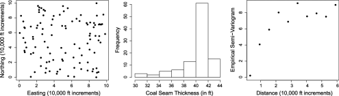
Figure 1: Coal seam data: Sampling locations, distribution of thickness, empirical semivariogram.

As a brief demonstration of the SFDEL method, we consider a coal seam dataset based on a SAS example (SAS2008 , Chapter 70). Figure 1 shows locations of 105 sampling sites and the corresponding distribution of coal seam thickness. Coal seam measurements often exhibit spatial smoothness (Journel and Huijbregts journel1978 , page 165), as also indicated in the empirical semivariogram in Figure 1 (found by binning distances into 10 bins up to half the maximum distance between points and plotting Matheron’s average over each bin against the bin midpoint). Following the SAS analysis, this suggests a Gaussian variogram model $2\gamma(\mathbf{h};\theta_{1},\theta_{2})=2\theta_{1}[1-\exp(-\|\mathbf{h}\|^{2}/\theta_{2}^{2})]$, $\mathbf{h}\in\mathbb{R}^{2}$, with scale $\theta_{1}>0$ and range $\theta_{2}>0$ parameters, though the present data are synthetic with a value $\theta_{2}=1$ as explained below.

Note that the spatial locations are not clearly uniform nor is the marginal distribution apparently normal. To fit the variogram model in a way that allows nonparametric confidence intervals (CIs) to access the precision of the estimated parameters, without making assumptions about the joint distribution of the data or the distribution of spatial locations, one can apply the SFDEL method using estimating functions as in Example 3 motivated by least squares estimation. Alternatively, one can apply a kernel bandwidth estimator of the varigoram for which large sample distributional results are recently known (García-Soidán gsoidan2007 , Maity and Sherman maity2012 ).

We focus on the range parameter $\theta_{2}$. Using a lag set $\mathbf{h}_{1}=(1/4,1/4)^{\prime}$, $\mathbf{h}_{2}=(1,1)^{\prime}$, $\mathbf{h}_{3}=(2,2)^{\prime}$ in SFDEL, motivated by empirical lags in Figure 1, the maximized SFDEL function produces a point estimate $\hat{\theta}_{2}=1.123$ ($\times 10\mbox{,}000$ ft) with a 90% SFDEL CI for $\theta_{2}$ as $(0.896,1.571)$. This arises from a frequency grid $\{\lambda_{n}^{-\kappa}\mathbf{j}\dvtx[-C^{*}\lambda_{n},C^{*}\lambda_{n}]^{2}\cap\mathbb{Z}^{2}\}$, $C^{*}=2$, $\kappa=0.2$ based on $\lambda_{n}=10$ for sampling region in Figure 1. With a larger frequency grid $C^{*}=4$, $\kappa=0.2$, the 90% SFDEL CI is similar $(0.887,1.378)$ with a point estimate $1.071$, and increasing the grid spacing $\kappa=0.1$ produces similar range estimates ($1.107$ and $1.101$ for $C^{*}=2,4$) and intervals. In contrast, using the lags above and the Nadaraya–Watson kernel estimator of the semivariogram $\hat{\gamma}(\mathbf{h})$ (based on the Epanechnikov kernel, cf. García-Soidán gsoidan2007 ), the range parameter estimates are $1.505,1.230,1.335$ for bandwidths $h=0.5,1,1.5$, where $h=0.5$ arises from MSE optimal order considerations. This approach can also produce large-sample nonparametric CIs based on normal limits for $\lambda_{n}[\hat{\gamma}(\mathbf{h})-\gamma(\mathbf{h})]$, having a covariance matrix $\mathcal{C}\cdot V$, $\mathcal{C}=[\int f^{2}]^{-2}\int f^{4}$, involving the unknown density $f$ of locations $\{\mathbf{s}_{i}/\lambda_{n}\}_{i=1}^{105}$ on $[0,1]^{2}$. For bandwidths $h=0.5,1,1.5$, the 90% CIs for $\theta_{2}$ are given by $(1.203,1.743)$, $(0.972,1.512)$, $(1.038,1.564)$ based on $\hat{\mathcal{C}}=1.23$ from bivariate kernel density estimation (cf. Venables and Ripley ripley2002 ) and simplifying the matrix $V$ by assuming the process is Gaussian (cf. García-Soidán gsoidan2007 , pages 490–491). Unlike CIs from kernel estimation, the SFDEL CIs require no variance or density approximation steps, tend to be less sensitive to tuning parameters, and all contain the true value $\theta_{2}=1$ here.

To provide some assessment of the CI methods, we conducted a small simulation study generating marginally standard normal variates $\{Y(\mathbf{s}_{i})\}_{i=1}^{105}$ with correlation $\operatorname{corr}[Y(\mathbf{s}),Y(\mathbf{s}+\mathbf{h})]=\exp(-\|\mathbf{h}\|^{2})$ at the locations $\{\mathbf{s}_{i}\}_{i=1}^{105}$ in Figure 1 and defining observations $\{Z(\mathbf{s}_{i})=\sqrt{\theta_{1}/2}[Y^{2}(\mathbf{s}_{i})-1]+40.23\}_{i=1}^{105}$ from a spatial process having a Gaussian variogram as above with scale $\theta_{1}=7.5$ and range $\theta_{2}=1$; this data-generation approximately matches features in the original SAS coal seam data and also produced the data example above. Based on 1000 simulations, 90% CIs for the range parameter $\theta_{2}$ from the SFDEL method had coverages $90.5,87.4,93.3$ for $C^{*}=2$ and $89.3,88.7,86.4$ for $C^{*}=4$, over grid spacings $\kappa=0.05,0.1,0.2$. In contrast, 90% CIs for $\theta_{2}$ from the kernel estimation approach had actual coverages $68.4,74.4,52.7$ for bandwidths $h=0.5,1,1.5$.

7 Proofs of the results

7.1 Notation and lemmas

Define the bias corrected periodogram$\tilde{I}_{n}(\bolds{\omega})={I}_{n}(\bolds{\omega})-n^{-1}\lambda_{n}^{d}\hat{\sigma}_{n}({\mathbf{0}})$ and its (unobservable) variant ${I}^{*}_{n}(\bolds{\omega})={I}_{n}(\bolds{\omega})-n^{-1}\lambda_{n}^{d}{\sigma}({\mathbf{0}})$. Recall that $A_{n}(\bolds{\omega})=c_{n}^{-1}{\sigma}({\mathbf{0}})+K\phi(\bolds{\omega})$, $\bolds{\omega}\in\mathbb{R}^{d}$, where $K=(2\pi)^{d}\int f^{2}$. For notational simplicity, for a random quantity $T$ depending on both $\{Z(\mathbf{s})\dvtx\mathbf{s}\in\mathbb{R}^{d}\}$ and $\{\mathbf{X}_{1},\mathbf{X}_{2},\ldots\}$, $ET$ will denote the conditional expectation of $T$ given $\mathbb{X}\equiv\{\mathbf{X}_{1},\mathbf{X}_{2},\ldots\}$ and likewise $P$ will denote conditional probability. Thus, in the following, $P(-2\log\mathcal{R}_{n}(\theta_{0})\leq t)$ in fact refers to

$$P\bigl{(}-2\log\mathcal{R}_{n}(\theta_{0})\leq t|\mathbb{X}\bigr{)},\qquad t>0.$$

Also, write $P_{\mathbf{X}}$ and $E_{\mathbf{X}}$ to denote the probability and the expectation under the joint distribution of $\mathbf{X}_{1},\mathbf{X}_{2},\ldots.$ Further, let $C$ or $C(\cdot)$ denote generic constants that depend on their arguments (if any), but do not depend on $n$ or the $\{\mathbf{X}_{i}\}$.

We now provide some lemmas that will be used for proving the main results of the paper. Proofs of the lemmas and Proposition 4.1 are relegated to the supplementary material supp to save space. For continuity, supplementary material supp begins with three technical lemmas (Lemmas 7.1–7.3), providing some general cumulant and integral inequalities as well as the bias and the variance of the periodogram $I_{n}(\cdot)$ that are used to establish Lemmas 7.4–7.7 below; these results may also be of independent interest. As presented next, Lemmas 7.4–7.7 deal with various properties and sums of the periodogram that we will need to analyze the asymptotic behavior of the SFDEL ratio statistic under different asymptotic structures and establish the main results in Section 7.2.

Lemma 7.4.

Under conditions (C.0)–(C.3) and (C.5)^′

$$E\Biggl{[}\sum_{k=1}^{N}G_{\theta_{0}}(\bolds{\omega}_{kn})G_{\theta_{0}}(\bolds{\omega}_{kn})^{\prime}I_{n}^{2}(\bolds{\omega}_{kn})\Biggr{]}$$

$$\qquad=2\sum_{k=1}^{N}G_{\theta_{0}}(\bolds{\omega}_{kn})G_{\theta_{0}}(\bolds{\omega}_{kn})^{\prime}A_{n}^{2}(\bolds{\omega}_{kn})+o\bigl{(}b_{n}^{2}\bigr{)}\qquad\mbox{a.s. ($P_{\mathbf{X}}$).}$$

Lemma 7.5.

Under conditions (C.0)–(C.3) and (C.5)^′,

$$\sum_{i=1}^{N}G_{\theta_{0}}(\bolds{\omega}_{in})G_{\theta_{0}}(\bolds{\omega}_{in})^{\prime}\bigl{[}\tilde{I}_{n}^{2}(\bolds{\omega}_{in})-\bigl{(}A_{n}^{2}(\bolds{\omega}_{in})+K^{2}\phi^{2}(\bolds{\omega}_{in})\bigr{)}\bigr{]}$$

$$\qquad=o_{p}\bigl{(}b_{n}^{2}\bigr{)}\qquad\mbox{a.s. ($P_{\mathbf{X}}$).}$$

Lemma 7.6.

Under conditions (C.0)–(C.3) and (C.5)^′, for any $\varepsilon>0$, $P(\max_{1\leq k\leq N}\|G_{\theta_{0}}(\bolds{\omega}_{kn})I_{n}(\bolds{\omega}_{kn})\|>\varepsilon b_{n})=o(1),\mbox{a.s. }(P_{\mathbf{X}})$.

Lemma 7.7.

Let $ch^{o}(B)$ denote the interior of the convex hull of a set $B\subset\mathbb{R}^{p}$. Under conditions (C.0)–(C.3) and (C.5)^′, it holds that, as $n\rightarrow\infty$, $P(0\in\mbox{ch}^{o}\{G_{\theta_{0}}(\bolds{\omega}_{kn})\tilde{I}_{n}(\bolds{\omega}_{kn})\}_{k=1}^{N})\rightarrow 1$ $\mbox{a.s. }(P_{\mathbf{X}})$.

7.2 Proofs of the main results

We now present the proofs of the results from Section 5. In the following, references to the equations from the supplementary material supp are given as (S.$*$).

Proof of Theorem 5.1 By Lemma 7.7, $\mathcal{R}_{n}(\theta_{0})$ exists and is positive on a set with probability tending to one, a.s. ($P_{\mathbf{X}}$). When $\mathcal{R}_{n}(\theta_{0})>0$ holds, by a general and standard EL result based on Lagrange multipliers (cf. Owen owen1988 , page 100), one can express $\mathcal{R}_{n}(\theta_{0})$ as

$$\mathcal{R}_{n}(\theta_{0})=\prod_{k=1}^{N}(1+\gamma_{k})^{-1},$$ (17)

where $\beta_{\theta_{0}}\equiv\beta_{\theta_{0},n}$ satisfies $F_{n}(\theta_{0},\beta_{\theta_{0}})=0$ for

$$F_{n}(\theta,\beta)\equiv N^{-1}\sum_{k=1}^{N}\frac{G_{\theta}(\bolds{\omega}_{kn})\tilde{I}_{n}(\bolds{\omega}_{kn})}{1+\beta^{\prime}G_{\theta}(\bolds{\omega}_{kn})\tilde{I}_{n}(\bolds{\omega}_{kn})}$$

and where $\gamma_{k}\equiv\gamma_{k,n}=\beta_{\theta_{0}}^{\prime}G_{\theta_{0}}(\bolds{\omega}_{kn})\tilde{I}_{n}(\bolds{\omega}_{kn})$ satisfies $|\gamma_{k}|<1$ for all $1\leq k\leq N$. To prove the theorem, it is enough to show that given any subsequence $\{n_{i}\}$, there exists a further subsequence $\{n_{k}\}$ of $\{n_{i}\}$ such that $-\log\mathcal{R}_{n_{k}}(\theta_{0})\stackrel{{\scriptstyle d}}{{\rightarrow}}\chi^{2}_{p}$. We use this line of argument because, as the proof indicates, the asymptotic expansion of $-\log\mathcal{R}_{n_{k}}(\theta_{0})$ involves mean-like quantities (e.g., term $J_{k}$ in the following) which may have differing (normal) limit distributions along different subsequences of $\{n_{k}\}$; nevertheless, the log-ratio statistic $-\log\mathcal{R}_{n}(\theta_{0})$ is shown to have a single, well-defined chi-square limit.

Note first that, under the PID structure here, it follows immediately from (C.3) [cf. (S.10)] that

$$\qquad b_{n}^{2}\sim Nc_{*}^{-2}\quad\mbox{and}\quad\Biggl{\|}\Sigma_{n}-2c_{*}^{-2}\bigl{[}{\sigma}(\mathbf{0})\bigr{]}^{2}\sum_{k=1}^{N}G_{\theta_{0}}(\bolds{\omega}_{kn})G_{\theta_{0}}(\bolds{\omega}_{kn})^{\prime}\Biggr{\|}=o(N)$$ (18)

[which is applied to show (20) from (19) next]. Fix a subsequence $\{n_{i}\}$. Then by (C.3)(iii) and the fact that $\|G_{\theta_{0}}(\bolds{\omega})\|\leq C$ for all $\bolds{\omega}\in\mathbb{R}^{d}$, it follows that there exist a subsequence $\{n_{k}\}$ of $\{n_{i}\}$ and a nonsingular matrix $\Gamma^{*}$ (possibly depending on $\{n_{k}\}$) such that

$$N^{-1}\sum_{j=1}^{N}G_{\theta_{0}}(\bolds{\omega}_{jn})G_{\theta_{0}}(\bolds{\omega}_{jn})^{\prime}\mathop{\rightarrow}\Gamma^{*}\qquad\mbox{through $\{n_{k}\}$.}$$ (19)

For simplicity, replace the subscript $n_{k}$ by $k$ and set $N_{k}\equiv N_{n_{k}}$, $\bolds{\omega}_{j}\equiv\bolds{\omega}_{j,n_{k}}$, $\gamma_{j}\equiv\gamma_{j,n_{k}}$ and $\beta_{\theta_{0}}\equiv\beta_{\theta_{0},n_{k}}$. Also, let $W_{k}=N_{k}^{-1}\sum_{j=1}^{N_{k}}G_{\theta_{0}}(\bolds{\omega}_{j})G_{\theta_{0}}(\bolds{\omega}_{j})^{\prime}\tilde{I}_{k}^{2}(\bolds{\omega}_{j})$ and $J_{k}=N_{k}^{-1}\sum_{j=1}^{N_{k}}G_{\theta_{0}}(\bolds{\omega}_{kn})\tilde{I}_{k}(\bolds{\omega}_{j})$. Then by (18), (19), condition (C.3) and Lemmas 7.5–7.6, we have, a.s. ($P_{\mathbf{X}}$),

$$|J_{k}|=O_{p}\bigl{(}N_{k}^{-1/2}\bigr{)}\quad\mbox{and}\quad\bigl{\|}W_{k}-(2N_{k})^{-1}\Sigma_{k}\bigr{\|}=o_{p}(1)$$ (20)

as $k\mathop{\rightarrow}\infty$. Since $N_{k}^{-1}\Sigma_{k}\mathop{\rightarrow}2[{\sigma}(\mathbf{0})]^{2}c_{*}^{-2}\Gamma^{*}$, $W_{k}$ is nonsingular whenever $\|W_{k}-[{\sigma}(\mathbf{0})]^{2}c_{*}^{-2}\Gamma^{*}\|$ is sufficiently small.

$\|\beta_{\theta_{0}}\|=O_{p}(N_{k}^{-1/2})$, a.s. ($P_{\mathbf{X}}$).

Write $\beta_{\theta_{0}}=t_{0}\mathbf{u}_{0}$ where $\|\mathbf{u}_{0}\|=1$ and $t_{0}=\|\beta_{\theta_{0}}\|$. Then

$$0 = \bigl{\|}F_{k}(\theta_{0},\beta_{\theta_{0}})\bigr{\|}\geq\bigl{|}\mathbf{u}_{0}^{\prime}F_{k}(\theta_{0},t_{\theta_{0}})\bigr{|}$$

$$= N_{k}^{-1}\Biggl{|}\mathbf{u}_{0}^{\prime}\Biggl{(}\sum_{j=1}^{N_{k}}G_{\theta_{0}}(\bolds{\omega}_{j})\tilde{I}_{k}(\bolds{\omega}_{j})-t_{0}\sum_{j=1}^{N_{k}}\frac{G_{\theta_{0}}(\bolds{\omega}_{j})\tilde{I}_{k}(\bolds{\omega}_{j})\mathbf{u}_{0}^{\prime}G_{\theta_{0}}(\bolds{\omega}_{j})\tilde{I}_{n}(\bolds{\omega}_{j})}{1+t_{0}\mathbf{u}_{0}^{\prime}G_{\theta_{0}}(\bolds{\omega}_{j})\tilde{I}_{n}(\bolds{\omega}_{j})}\Biggr{)}\Biggr{|}$$

$$\geq \frac{t_{0}\mathbf{u}_{0}^{\prime}W_{k}\mathbf{u}_{0}}{1+t_{0}Y_{k}}-\sum_{j=1}^{p}\bigl{|}\mathbf{e}_{j}^{\prime}J_{k}\bigr{|},$$

where $Y_{k}=\max_{1\leq j\leq N_{k}}\|G_{\theta_{0}}(\bolds{\omega}_{j})\||\tilde{I}_{k}(\bolds{\omega}_{j})|$ and $\mathbf{e}_{1},\ldots,\mathbf{e}_{r}$ denote the standard basis of $\mathbb{R}^{r}$, with $\mathbf{e}_{i}\in\mathbb{R}^{r}$ having a $1$ in the $i$th position and $0$ elsewhere. By Lemma 7.6, $Y_{k}=o_{p}(N_{k}^{1/2})$. Also, using (20), one can conclude that $\mathbf{u}_{0}^{\prime}W_{k}\mathbf{u}_{0}\geq{\sigma}_{0}^{*}+o_{p}(1)$ and hence, $(1+t_{0}Y_{k})^{-1}t_{0}=O_{p}(N_{k}^{-1/2})$, a.s. ($P_{\mathbf{X}}$), where ${\sigma}^{*}_{0}>0$ is the smallest eigenvalue of $[{\sigma}(\mathbf{0})]^{2}c_{*}^{-2}\Gamma^{*}$. Hence, it follows that $t_{0}=\|\beta_{\theta_{0}}\|=O_{p}(N_{k}^{-1/2})$, proving the claim.

By the Claim and Lemma 7.6,

$$\quad\max_{1\leq j\leq N_{k}}|\gamma_{j}|\leq\|\beta_{\theta_{0}}\|Y_{k}=O_{p}\bigl{(}N_{k}^{-1/2}\bigr{)}o_{p}\bigl{(}N_{k}^{1/2}\bigr{)}=o_{p}(1)\qquad\mbox{a.s. ($P_{\mathbf{X}}$).}$$ (21)

Next, we obtain a stochastic approximation to $\beta_{\theta_{0}}$. Using $F_{k}(\theta_{0},\beta_{\theta_{0}})=0$, note that

$$0 = N_{k}^{-1}\sum_{j=1}^{N_{k}}\frac{G_{\theta_{0}}(\bolds{\omega}_{j})\tilde{I}_{k}(\bolds{\omega}_{j})}{1+\beta_{\theta_{0}}^{\prime}G_{\theta_{0}}(\bolds{\omega}_{j})\tilde{I}_{n}(\bolds{\omega}_{j})}$$

$$= N_{k}^{-1}\sum_{j=1}^{N_{k}}G_{\theta_{0}}(\bolds{\omega}_{j})\tilde{I}_{n}(\bolds{\omega}_{j})\biggl{[}1-\gamma_{j}+\frac{\gamma_{j}^{2}}{1+\gamma_{j}}\biggr{]}$$

$$= J_{k}-W_{k}\beta_{\theta_{0}}+N_{k}^{-1}\sum_{j=1}^{N_{k}}\frac{G_{\theta_{0}}(\bolds{\omega}_{j})\tilde{I}_{k}(\bolds{\omega}_{j})\gamma_{j}^{2}}{1+\gamma_{j}}.$$

Therefore, we have the representation

$$\beta_{\theta_{0}}=(W_{k})^{-1}J_{k}+\eta_{k},$$ (22)

where, using condition (C.3), Lemma 7.5, the Claim, and (21), $\|\eta_{k}\|\leq$ $Y_{k}\|\beta_{\theta_{0}}\|^{2}\|W_{k}\|^{-1}\{N_{k}^{-1}\sum_{j=1}^{N_{k}}\|G_{\theta_{0}}(\bolds{\omega}_{j})\|^{2}\tilde{I}_{k}^{2}(\bolds{\omega}_{j})\}\{\max_{1\leq j\leq N_{k}}(1-|\gamma_{j}|)^{-1}\}=o_{p}(N_{k}^{1/2})O_{p}(N_{k}^{-1})O_{p}(1)O_{p}(1)O_{p}(1)=o_{p}(N_{k}^{-1/2})$, a.s. ($P_{\mathbf{X}}$). For $\|\beta_{\theta_{0}}\|Y_{k}<1$, applying a Taylor series expansion, we have

$$\log{(1+\gamma_{j})}=\gamma_{j}-\gamma_{j}^{2}/2+\Delta_{j},$$

where $|\Delta_{j}|\leq\|\beta_{\theta_{0}}\|^{3}Y_{k}\|G_{\theta_{0}}(\bolds{\omega}_{j})\|^{2}\tilde{I}_{k}^{2}(\bolds{\omega}_{j})(1-\|\beta_{\theta_{0}}\|Y_{k})^{-3}$ for all $1\leq j\leq N_{k}$. Also, by Lemmas 7.4–7.5, (C.3) and (20), $N_{k}J_{k}^{\prime}(W_{k})^{-1}J_{k}\stackrel{{\scriptstyle d}}{{\longrightarrow}}2\chi^{2}_{p}$ and

$$\sum_{j=1}^{N_{k}}|\Delta_{j}| \leq N_{k}\|\beta_{\theta_{0}}\|^{3}Y_{k}\bigl{(}1-\|\beta_{\theta_{0}}\|Y_{k}\bigr{)}^{-3}\Biggl{\{}N_{k}^{-1}\sum_{j=1}^{N_{k}}\bigl{\|}G_{\theta_{0}}(\bolds{\omega}_{j})\bigr{\|}^{2}\tilde{I}_{k}^{2}(\bolds{\omega}_{j})\Biggr{\}}$$

$$= N_{k}O_{p}\bigl{(}N_{k}^{-3/2}\bigr{)}o_{p}\bigl{(}N_{k}^{1/2}\bigr{)}O_{p}(1)O_{p}(1)=o_{p}(1),$$

a.s. ($P_{\mathbf{X}}$). Hence, it follows that

$$-\log\mathcal{R}_{n_{k}}(\theta_{0}) \equiv -\log\mathcal{R}_{k}(\theta_{0})=\sum_{j=1}^{N_{k}}\log{(1+\gamma_{j})}$$

$$= \Biggl{[}\sum_{j=1}^{N_{k}}\gamma_{j}-2^{-1}\sum_{j=1}^{N_{k}}\gamma_{j}^{2}\Biggr{]}+\sum_{j=1}^{N_{k}}\Delta_{j}$$

$$= \bigl{[}\beta_{\theta_{0}}^{\prime}[N_{k}J_{k}]-2^{-1}N_{k}\beta_{\theta_{0}}^{\prime}W_{k}\beta_{\theta_{0}}\bigr{]}+\sum_{j=1}^{N_{k}}\Delta_{j}$$

$$= 2^{-1}N_{k}J_{k}^{\prime}(W_{k})^{-1}J_{k}+o_{p}(1)\stackrel{{\scriptstyle d}}{{\longrightarrow}}\chi^{2}_{p}.$$

This completes the proof of Theorem 5.1.

Proof of Theorem 5.2 By conditions on $c_{n}$, $N$ and $\lambda_{n}$ in the MID case of part (a),

$$b_{n}^{2} \sim Nc_{n}^{-2}\quad\mbox{and}$$

$$\Biggl{\|}\Sigma_{n}-2c_{n}^{-2}\bigl{[}{\sigma}(\mathbf{0})\bigr{]}^{2}\sum_{k=1}^{N}G_{\theta_{0}}(\bolds{\omega}_{kn})G_{\theta_{0}}(\bolds{\omega}_{kn})^{\prime}\Biggr{\|} = o\bigl{(}b_{n}^{2}\bigr{)},\vspace*{2pt}$$

where $c_{n}^{-1}=o(1)$. Thus, $b_{n}$ has a slower growth rate in this case compared to the PID case. As in the proof of Theorem 5.1, it is enough to show that $-\log\mathcal{R}_{n_{k}}(\theta_{0})\stackrel{{\scriptstyle d}}{{\longrightarrow}}\chi^{2}_{p}$ through some subsequence $\{n_{k}\}$ of a given subsequence $\{n_{i}\}$. Indeed, the subsequence $\{n_{k}\}$ is extracted using (C.3)(iii) as before so that (19) holds. Let $Y_{k}$, $\beta_{\theta_{0}}$ and $\gamma_{j}$ be as defined in the proof of Theorem 5.1, and here we continue to use the convention that the subscript $n_{k}$ is replaced by $k$, as before. Next, redefine $J_{k}$ and $W_{k}$ as $J_{k}=b_{k}^{-2}\sum_{j=1}^{N_{k}}G_{\theta_{0}}(\bolds{\omega}_{kn})\tilde{I}_{k}(\bolds{\omega}_{j})$ and $W_{k}=b_{k}^{-2}\sum_{j=1}^{N_{k}}G_{\theta_{0}}(\bolds{\omega}_{j})G_{\theta_{0}}(\bolds{\omega}_{j})^{\prime}\tilde{I}_{k}^{2}(\bolds{\omega}_{j})$ where, following the convention, we write $b_{k}=b_{n_{k}}$. Then, by (19), (7.2), Lemma 7.5 and (C.4),

$$\bigl{\|}W_{k}-\bigl{[}{\sigma}(\mathbf{0})\bigr{]}^{2}\Gamma^{*}\bigr{\|} = o(1)\quad\mbox{and}$$

$$b_{k}J_{k} \stackrel{{\scriptstyle d}}{{\longrightarrow}} N\bigl{(}0,2\bigl{[}{\sigma}(\mathbf{0})\bigr{]}^{2}\Gamma^{*}\bigr{)}.$$

Further, retracing the proof of Theorem 5.1 and using Lemmas 7.5–7.7, one can conclude that a.s. ($P_{\mathbf{X}}$), $\|\beta_{\theta_{0}}\|=O_{p}(b_{k}^{-1})$ (cf. the Claim), $\max\{|\gamma_{j}|\dvtx 1\leq j\leq N_{k}\}=o_{p}(1)$ [cf. (21)] and the representation (22) holds with $\eta_{k}=o_{p}(b_{k}^{-1})$. Hence, it follows that

$$-\log\mathcal{R}_{k}(\theta_{0}) = \Biggl{[}\sum_{j=1}^{N_{k}}\gamma_{j}-2^{-1}\sum_{j=1}^{N_{k}}\gamma_{j}^{2}\Biggr{]}+\sum_{j=1}^{N_{k}}\Delta_{j}$$

$$= \bigl{[}\beta_{\theta_{0}}^{\prime}\bigl{[}b_{k}^{2}J_{k}\bigr{]}-2^{-1}b_{k}^{2}\beta_{\theta_{0}}^{\prime}W_{k}\beta_{\theta_{0}}\bigr{]}+\sum_{j=1}^{N_{k}}\Delta_{j}$$

$$= 2^{-1}b_{k}^{2}J_{k}^{\prime}(W_{k})^{-1}J_{k}+o_{p}(1)\stackrel{{\scriptstyle d}}{{\longrightarrow}}\chi^{2}_{p}.$$

This completes the proof of Theorem 5.2(a).

Next, consider part (b). Note that in this MID case, $Nc_{n}^{-2}\ll\lambda_{n}^{\kappa d}$ and hence, $b_{n}^{2}\sim\lambda_{n}^{\kappa d}$. Also, using the boundedness of $\|G_{\theta_{0}}(\cdot)\|$ over $\mathbb{R}^{d}$ and conditions (C.3)(i), (ii), (iv) and the DCT, one gets

$$\bigl{\|}\Sigma_{n}-2\lambda_{n}^{\kappa d}\Gamma\bigr{\|}=o\bigl{(}\lambda_{n}^{\kappa d}\bigr{)},$$

where $\Gamma\equiv\int G_{\theta_{0}}(\bolds{\omega})G_{\theta_{0}}(\bolds{\omega})^{\prime}K^{2}\phi^{2}(\bolds{\omega})\,d\bolds{\omega}$ is nonsingular. Now retracing the proofs of Theorems 5.1 and 5.2(a) (with $\{n_{k}\}$ replaced by the full sequence $\{n\}$), one can show that $-2\log\mathcal{R}_{n}(\theta_{0})=b_{n}^{2}J_{0n}^{\prime}(W_{0n})^{-1}J_{0n}+o_{p}(1)$, where $J_{0n}=b_{n}^{-2}\sum_{j=1}^{N}G_{\theta_{0}}(\bolds{\omega}_{jn})\tilde{I}_{n}(\bolds{\omega}_{j})$ and $W_{0n}=b_{n}^{-2}\sum_{j=1}^{N}G_{\theta_{0}}(\bolds{\omega}_{jn})G_{\theta_{0}}(\bolds{\omega}_{jn})^{\prime}\tilde{I}_{n}^{2}(\bolds{\omega}_{jn})$. Note that by Lemma 7.5 and the fact that $b_{n}^{2}\sim\lambda_{n}^{\kappa d}$, we have

$$\bigl{\|}W_{n}-b_{n}^{-2}\Sigma_{n}\bigr{\|}=o(1),$$

which is different from the previous two cases covered by Theorems 5.1 and 5.2(a) [where $\|W_{n}-2^{-1}(b_{n}^{-2}\Sigma_{n})\|=o(1)$]. In view of (C.4), this implies that $b_{n}^{2}J_{0n}^{\prime}(W_{0n})^{-1}J_{0n}\stackrel{{\scriptstyle d}}{{\longrightarrow}}\chi^{2}_{p}$, proving part (b).

Remark 7.1.

From the proof of Theorems 5.1–5.2, it follows that the different scalings in the two cases are required by the dominant term in the asymptotic variance of the sum $\sum_{k=1}^{N}G_{\theta_{0}}(\bolds{\omega}_{kn})I_{n}^{*}(\bolds{\omega}_{kn})$ and the automatic variance stabilization factor, both of which arise from the inner mechanics of the SFDEL. Under PID and under “slow” MID, the leading term is given by $Nc_{n}^{-1}{\sigma}(\mathbf{0})$, which is of a larger order of magnitude than $\lambda_{n}^{\kappa d}$. When the infilling rate is high, that is, $Nc_{n}^{-2}\ll\lambda_{n}^{\kappa d}$, the other term involving the spectral density of the $Z(\cdot)$-process dominates (as in the case of regularly spaced time series FDEL) and the standard scaling by $-2$ is appropriate.

Proof of Theorem 5.3 By Lemma 7.5 and the fact that $\hat{{\sigma}}_{n}(\mathbf{0})-{\sigma}(\mathbf{0})=O_{p}(\lambda_{n}^{-d/2})$ (cf. Lahiri lahiri2003a ), under the conditions of Theorem 5.2(b),

$$a_{n}(\theta_{0}) = \frac{b_{n}^{-2}\sum_{j=1}^{N}\|G_{\theta_{0}}(\bolds{\omega}_{jn})\|^{2}\tilde{I}_{n}^{2}(\bolds{\omega}_{jn})}{b_{n}^{-2}\sum_{j=1}^{N}\|G_{\theta_{0}}(\bolds{\omega}_{jn})\|^{2}I_{n}^{2}(\bolds{\omega}_{jn})}$$

$$= \frac{b_{n}^{-2}\sum_{j=1}^{N}\|G_{\theta_{0}}(\bolds{\omega}_{jn})\|^{2}[2K^{2}\phi^{2}(\bolds{\omega}_{jn})]+o_{p}(1)}{b_{n}^{-2}\sum_{j=1}^{N}\|G_{\theta_{0}}(\bolds{\omega}_{jn})\|^{2}[2K^{2}\phi^{2}(\bolds{\omega}_{jn})]+o_{p}(1)}=1+o_{p}(1)$$

while under the conditions of Theorems 5.1 and 5.2,

$$a_{n_{k}}(\theta_{0}) = \frac{b_{k}^{-2}\sum_{j=1}^{N_{k}}\|G_{\theta_{0}}(\bolds{\omega}_{k})\|^{2}[c_{n_{k}}^{-2}[{\sigma}(\mathbf{0})]^{2}]+o_{p}(1)}{b_{k}^{-2}\sum_{j=1}^{N_{k}}\|G_{\theta_{0}}(\bolds{\omega}_{k})\|^{2}[2c_{n_{k}}^{-2}[{\sigma}(\mathbf{0})]^{2}]+o_{p}(1)}$$

$$= 2^{-1}\bigl{(}1+o_{p}(1)\bigr{)}.$$

Now combining this with the proofs of Theorems 5.1–5.2, one can complete the proof of Theorem 5.3.

References

- (1) {barticle}[mr] \bauthor\bsnmBandyopadhyay, \bfnmS.\binitsS. and \bauthor\bsnmLahiri, \bfnmS. N.\binitsS. N. (\byear2009). \btitleAsymptotic properties of discrete Fourier transforms for spatial data. \bjournalSankhyā \bvolume71 \bpages221–259. \bidissn=0972-7671, mr=2639292 \bptnotecheck year \bptokimsref\endbibitem
- (2) {bmisc}[author] \bauthor\bsnmBandyopadhyay, \bfnmS.\binitsS., \bauthor\bsnmLahiri, \bfnmS. N.\binitsS. N. and \bauthor\bsnmNordman, \bfnmD. J.\binitsD. J. (\byear2013). \bhowpublishedA central limit theorem for periodogram based statistics for irregularly spaced spatial data and Whittle estimation. Preprint. \bptokimsref\endbibitem
- (3) {bmisc}[author] \bauthor\bsnmBandyopadhyay, \bfnmS.\binitsS., \bauthor\bsnmLahiri, \bfnmS. N.\binitsS. N. and \bauthor\bsnmNordman, \bfnmD. J.\binitsD. J. (\byear2015). \bhowpublishedSupplement to “A frequency domain empirical likelihood method for irregularly spaced spatial data.” DOI:\doiurl10.1214/14-AOS1291SUPP. \bptokimsref \endbibitem
- (4) {barticle}[mr] \bauthor\bsnmBradley, \bfnmRichard C.\binitsR. C. (\byear1989). \btitleA caution on mixing conditions for random fields. \bjournalStatist. Probab. Lett. \bvolume8 \bpages489–491. \biddoi=10.1016/0167-7152(89)90032-1, issn=0167-7152, mr=1040812 \bptokimsref\endbibitem
- (5) {barticle}[mr] \bauthor\bsnmBradley, \bfnmRichard C.\binitsR. C. (\byear1993). \btitleEquivalent mixing conditions for random fields. \bjournalAnn. Probab. \bvolume21 \bpages1921–1926. \bidissn=0091-1798, mr=1245294 \bptokimsref\endbibitem
- (6) {bbook}[mr] \bauthor\bsnmBrockwell, \bfnmPeter J.\binitsP. J. and \bauthor\bsnmDavis, \bfnmRichard A.\binitsR. A. (\byear1991). \btitleTime Series: Theory and Methods, \bedition2nd ed. \bpublisherSpringer, \blocationNew York. \biddoi=10.1007/978-1-4419-0320-4, mr=1093459 \bptokimsref\endbibitem
- (7) {bbook}[mr] \bauthor\bsnmCressie, \bfnmNoel A. C.\binitsN. A. C. (\byear1993). \btitleStatistics for Spatial Data. \bpublisherWiley, \blocationNew York. \bidmr=1239641 \bptokimsref\endbibitem
- (8) {bbook}[mr] \bauthor\bsnmDoukhan, \bfnmPaul\binitsP. (\byear1994). \btitleMixing: Properties and Examples. \bseriesLecture Notes in Statistics \bvolume85. \bpublisherSpringer, \blocationNew York. \biddoi=10.1007/978-1-4612-2642-0, mr=1312160 \bptokimsref\endbibitem
- (9) {barticle}[mr] \bauthor\bsnmDu, \bfnmJuan\binitsJ., \bauthor\bsnmZhang, \bfnmHao\binitsH. and \bauthor\bsnmMandrekar, \bfnmV. S.\binitsV. S. (\byear2009). \btitleFixed-domain asymptotic properties of tapered maximum likelihood estimators. \bjournalAnn. Statist. \bvolume37 \bpages3330–3361. \biddoi=10.1214/08-AOS676, issn=0090-5364, mr=2549562 \bptokimsref\endbibitem
- (10) {barticle}[mr] \bauthor\bsnmFuentes, \bfnmMontserrat\binitsM. (\byear2006). \btitleTesting for separability of spatial–temporal covariance functions. \bjournalJ. Statist. Plann. Inference \bvolume136 \bpages447–466. \biddoi=10.1016/j.jspi.2004.07.004, issn=0378-3758, mr=2211349 \bptokimsref\endbibitem
- (11) {barticle}[mr] \bauthor\bsnmFuentes, \bfnmMontserrat\binitsM. (\byear2007). \btitleApproximate likelihood for large irregularly spaced spatial data. \bjournalJ. Amer. Statist. Assoc. \bvolume102 \bpages321–331. \biddoi=10.1198/016214506000000852, issn=0162-1459, mr=2345545 \bptokimsref\endbibitem
- (12) {barticle}[mr] \bauthor\bsnmGarcía-Soidán, \bfnmPilar\binitsP. (\byear2007). \btitleAsymptotic normality of the Nadaraya–Watson semivariogram estimators. \bjournalTEST \bvolume16 \bpages479–503. \biddoi=10.1007/s11749-006-0016-8, issn=1133-0686, mr=2365173 \bptokimsref\endbibitem
- (13) {barticle}[author] \bauthor\bsnmHall, \bfnmPeter\binitsP. and \bauthor\bsnmLa Scala, \bfnmBarbara\binitsB. (\byear1990). \btitleMethodology and algorithms of empirical likelihood. \bjournalInt. Statist. Rev. \bvolume58 \bpages109–127. \bptokimsref\endbibitem
- (14) {barticle}[mr] \bauthor\bsnmHall, \bfnmPeter\binitsP. and \bauthor\bsnmPatil, \bfnmPrakash\binitsP. (\byear1994). \btitleProperties of nonparametric estimators of autocovariance for stationary random fields. \bjournalProbab. Theory Related Fields \bvolume99 \bpages399–424. \biddoi=10.1007/BF01199899, issn=0178-8051, mr=1283119 \bptokimsref\endbibitem
- (15) {barticle}[mr] \bauthor\bsnmIm, \bfnmHae Kyung\binitsH. K., \bauthor\bsnmStein, \bfnmMichael L.\binitsM. L. and \bauthor\bsnmZhu, \bfnmZhengyuan\binitsZ. (\byear2007). \btitleSemiparametric estimation of spectral density with irregular observations. \bjournalJ. Amer. Statist. Assoc. \bvolume102 \bpages726–735. \biddoi=10.1198/016214507000000220, issn=0162-1459, mr=2381049 \bptokimsref\endbibitem
- (16) {bbook}[author] \bauthor\bsnmJournel, \bfnmA. G.\binitsA. G. and \bauthor\bsnmHuijbregts, \bfnmC. J.\binitsC. J. (\byear1978). \btitleMining Geostatistics. \bpublisherAcademic Press, \blocationSan Diego, CA. \bptokimsref\endbibitem
- (17) {barticle}[mr] \bauthor\bsnmKitamura, \bfnmYuichi\binitsY. (\byear1997). \btitleEmpirical likelihood methods with weakly dependent processes. \bjournalAnn. Statist. \bvolume25 \bpages2084–2102. \biddoi=10.1214/aos/1069362388, issn=0090-5364, mr=1474084 \bptokimsref\endbibitem
- (18) {barticle}[mr] \bauthor\bsnmLahiri, \bfnmS. N.\binitsS. N. (\byear2003). \btitleCentral limit theorems for weighted sums of a spatial process under a class of stochastic and fixed designs. \bjournalSankhyā \bvolume65 \bpages356–388. \bidissn=0972-7671, mr=2028905 \bptokimsref\endbibitem
- (19) {barticle}[mr] \bauthor\bsnmLahiri, \bfnmS. N.\binitsS. N. (\byear2003). \btitleA necessary and sufficient condition for asymptotic independence of discrete Fourier transforms under short- and long-range dependence. \bjournalAnn. Statist. \bvolume31 \bpages613–641. \biddoi=10.1214/aos/1051027883, issn=0090-5364, mr=1983544 \bptokimsref\endbibitem
- (20) {barticle}[mr] \bauthor\bsnmLahiri, \bfnmSoumendra Nath\binitsS. N., \bauthor\bsnmLee, \bfnmYoondong\binitsY. and \bauthor\bsnmCressie, \bfnmNoel\binitsN. (\byear2002). \btitleOn asymptotic distribution and asymptotic efficiency of least squares estimators of spatial variogram parameters. \bjournalJ. Statist. Plann. Inference \bvolume103 \bpages65–85. \biddoi=10.1016/S0378-3758(01)00198-7, issn=0378-3758, mr=1896984 \bptokimsref\endbibitem
- (21) {barticle}[mr] \bauthor\bsnmLahiri, \bfnmS. N.\binitsS. N. and \bauthor\bsnmMukherjee, \bfnmKanchan\binitsK. (\byear2004). \btitleAsymptotic distributions of -estimators in a spatial regression model under some fixed and stochastic spatial sampling designs. \bjournalAnn. Inst. Statist. Math. \bvolume56 \bpages225–250. \biddoi=10.1007/BF02530543, issn=0020-3157, mr=2067154 \bptokimsref\endbibitem
- (22) {barticle}[mr] \bauthor\bsnmLoh, \bfnmWei-Liem\binitsW.-L. (\byear2005). \btitleFixed-domain asymptotics for a subclass of Matérn-type Gaussian random fields. \bjournalAnn. Statist. \bvolume33 \bpages2344–2394. \biddoi=10.1214/009053605000000516, issn=0090-5364, mr=2211089 \bptokimsref\endbibitem
- (23) {barticle}[mr] \bauthor\bsnmMaity, \bfnmArnab\binitsA. and \bauthor\bsnmSherman, \bfnmMichael\binitsM. (\byear2012). \btitleTesting for spatial isotropy under general designs. \bjournalJ. Statist. Plann. Inference \bvolume142 \bpages1081–1091. \biddoi=10.1016/j.jspi.2011.11.013, issn=0378-3758, mr=2879753 \bptokimsref\endbibitem
- (24) {barticle}[mr] \bauthor\bsnmMatsuda, \bfnmYasumasa\binitsY. and \bauthor\bsnmYajima, \bfnmYoshihiro\binitsY. (\byear2009). \btitleFourier analysis of irregularly spaced data on . \bjournalJ. R. Stat. Soc. Ser. B Stat. Methodol. \bvolume71 \bpages191–217. \biddoi=10.1111/j.1467-9868.2008.00685.x, issn=1369-7412, mr=2655530 \bptokimsref\endbibitem
- (25) {barticle}[mr] \bauthor\bsnmMonti, \bfnmAnna Clara\binitsA. C. (\byear1997). \btitleEmpirical likelihood confidence regions in time series models. \bjournalBiometrika \bvolume84 \bpages395–405. \biddoi=10.1093/biomet/84.2.395, issn=0006-3444, mr=1467055 \bptokimsref\endbibitem
- (26) {barticle}[mr] \bauthor\bsnmNordman, \bfnmDaniel J.\binitsD. J. (\byear2008). \btitleA blockwise empirical likelihood for spatial lattice data. \bjournalStatist. Sinica \bvolume18 \bpages1111–1129. \bidissn=1017-0405, mr=2440078 \bptokimsref\endbibitem
- (27) {barticle}[mr] \bauthor\bsnmNordman, \bfnmDaniel J.\binitsD. J. (\byear2008). \btitleAn empirical likelihood method for spatial regression. \bjournalMetrika \bvolume68 \bpages351–363. \biddoi=10.1007/s00184-007-0167-y, issn=0026-1335, mr=2448966 \bptokimsref\endbibitem
- (28) {barticle}[mr] \bauthor\bsnmNordman, \bfnmDaniel J.\binitsD. J. and \bauthor\bsnmCaragea, \bfnmPetruţa C.\binitsP. C. (\byear2008). \btitlePoint and interval estimation of variogram models using spatial empirical likelihood. \bjournalJ. Amer. Statist. Assoc. \bvolume103 \bpages350–361. \biddoi=10.1198/016214507000001391, issn=0162-1459, mr=2420238 \bptokimsref\endbibitem
- (29) {barticle}[mr] \bauthor\bsnmNordman, \bfnmDaniel J.\binitsD. J. and \bauthor\bsnmLahiri, \bfnmSoumendra N.\binitsS. N. (\byear2004). \btitleOn optimal spatial subsample size for variance estimation. \bjournalAnn. Statist. \bvolume32 \bpages1981–2027. \biddoi=10.1214/009053604000000779, issn=0090-5364, mr=2102500 \bptokimsref\endbibitem
- (30) {barticle}[mr] \bauthor\bsnmNordman, \bfnmDaniel J.\binitsD. J. and \bauthor\bsnmLahiri, \bfnmSoumendra N.\binitsS. N. (\byear2006). \btitleA frequency domain empirical likelihood for short- and long-range dependence. \bjournalAnn. Statist. \bvolume34 \bpages3019–3050. \biddoi=10.1214/009053606000000902, issn=0090-5364, mr=2329476 \bptokimsref\endbibitem
- (31) {barticle}[mr] \bauthor\bsnmNordman, \bfnmDaniel J.\binitsD. J., \bauthor\bsnmLahiri, \bfnmSoumendra N.\binitsS. N. and \bauthor\bsnmFridley, \bfnmBrooke L.\binitsB. L. (\byear2007). \btitleOptimal block size for variance estimation by a spatial block bootstrap method. \bjournalSankhyā \bvolume69 \bpages468–493. \bidissn=0972-7671, mr=2460005 \bptokimsref\endbibitem
- (32) {barticle}[mr] \bauthor\bsnmOwen, \bfnmArt\binitsA. (\byear1990). \btitleEmpirical likelihood ratio confidence regions. \bjournalAnn. Statist. \bvolume18 \bpages90–120. \biddoi=10.1214/aos/1176347494, issn=0090-5364, mr=1041387 \bptokimsref\endbibitem
- (33) {barticle}[mr] \bauthor\bsnmOwen, \bfnmArt B.\binitsA. B. (\byear1988). \btitleEmpirical likelihood ratio confidence intervals for a single functional. \bjournalBiometrika \bvolume75 \bpages237–249. \biddoi=10.1093/biomet/75.2.237, issn=0006-3444, mr=0946049 \bptokimsref\endbibitem
- (34) {bbook}[author] \bauthor\bsnmOwen, \bfnmArt B.\binitsA. B. (\byear2001). \btitleEmpirical Likelihood. \bpublisherCRC Press, \blocationBoca Raton, FL. \bptokimsref\endbibitem
- (35) {barticle}[mr] \bauthor\bsnmQin, \bfnmJing\binitsJ. and \bauthor\bsnmLawless, \bfnmJerry\binitsJ. (\byear1994). \btitleEmpirical likelihood and general estimating equations. \bjournalAnn. Statist. \bvolume22 \bpages300–325. \biddoi=10.1214/aos/1176325370, issn=0090-5364, mr=1272085 \bptokimsref\endbibitem
- (36) {bbook}[author] \bauthor\bsnmSAS (\byear2008). \btitleSAS/STAT(R) 9.2 User’s Guide. \bpublisherSAS Institute, \blocationCary, NC. \bptokimsref\endbibitem
- (37) {barticle}[mr] \bauthor\bsnmStein, \bfnmMichael\binitsM. (\byear1989). \btitleAsymptotic distributions of minimum norm quadratic estimators of the covariance function of a Gaussian random field. \bjournalAnn. Statist. \bvolume17 \bpages980–1000. \biddoi=10.1214/aos/1176347252, issn=0090-5364, mr=1015134 \bptokimsref\endbibitem
- (38) {bbook}[author] \bauthor\bsnmVenables, \bfnmW. N.\binitsW. N. and \bauthor\bsnmRipley, \bfnmB. D.\binitsB. D. (\byear2002). \btitleModern Applied Statistics with S, \bedition4th ed. \bpublisherSpringer, \blocationNew York. \bptokimsref\endbibitem
- (39) {barticle}[author] \bauthor\bsnmWilks, \bfnmSamuel S.\binitsS. S. (\byear1938). \btitleThe large-sample distribution of the likelihood ratio for testing composite hypotheses. \bjournalAnn. Math. Statist. \bvolume9 \bpages60–62. \bptokimsref\endbibitem
- (40) {barticle}[mr] \bauthor\bsnmZhang, \bfnmHao\binitsH. and \bauthor\bsnmZimmerman, \bfnmDale L.\binitsD. L. (\byear2005). \btitleTowards reconciling two asymptotic frameworks in spatial statistics. \bjournalBiometrika \bvolume92 \bpages921–936. \biddoi=10.1093/biomet/92.4.921, issn=0006-3444, mr=2234195 \bptokimsref\endbibitem