Contactless heat flux control with photonic devices

Abstract

The ability to control electric currents in solids using diodes and transistors is undoubtedly at the origin of the main developments in modern electronics which have revolutionized the daily life in the second half of 20th century. Surprisingly, until the year 2000 no thermal counterpart for such a control had been proposed. Since then, based on pioneering works on the control of phononic heat currents new devices were proposed which allow for the control of heat fluxes carried by photons rather than phonons or electrons. The goal of the present paper is to summarize the main advances achieved recently in the field of thermal energy control with photons.

I Introduction

The diode and the transistor introduced by F. Braun Braun and Bardeen et al. Bardeen (based on the works of Julius E. Lilienfeld from 1925), in 1874 and 1948 are the main building blocks of almost all modern systems of information treatment. These elementary devices allow for rectifying, switching, modulating and even amplifying the electric current in solids. Similar devices which would provide the same degree of control of heat currents instead of the control of electric currents are not as widespread in our daily life and the concepts for such devices for heat flow management at the nanoscale were introduced as recently as about ten years ago. In 2006 Baowen Li et al. Casati1 have proposed a thermal counterpart of a field-effect transistor. In this device the temperature bias plays the role of the voltage bias and the heat currents carried by phonons play the role of the electric currents. Later, several prototypes of phononic thermal logic gates BaowenLi2 as well as thermal memories BaowenLi3 ; BaowenLiEtAl2012 have been developed in order to process information by phononic heat currents rather than by electric currents.

However, this technology suffers from some weaknesses of fundamental nature which intrinsically limit its performance. One of the main limitations comes probably from the speed of acoustic phonons (heat carriers) which is four or five orders of magnitude smaller than the speed of light and therefore also some orders of magnitude smaller than the speed of electrons. Another intrinsic limitation of phononic devices is related to the inevitable presence of local Kapitza resistances. These resistances which originate from the mismatch of vibrational modes at the interface of different elements can reduce the phononic heat flow dramatically. Finally, the strong nonlinear phonon-phonon interaction mechanism makes the phononic devices difficult to deal with in presence of a strong thermal gradient. On the contrary the physics of energy transport mediated by photons instead of phonons remains unchanged close and far from thermal equilibrium. These limitations and difficulties explain, in part, why so many efforts have been deployed, during the last decades, to develop full optical or at least opto-electronic architectures for processing and managing information. Particularly important developments have been carried out during the last decade with plasmonics systems Ozbay ; Caglayan with the goal to increase the speed of information processing substantially while reducing the dimension of devices to the nanoscale at the same time.

In this paper we review the recent developments made to achieve a control of heat flow with contactless devices using thermal photons. We discuss the operating principles of the three basic building blocks for heat flow management which are the photonic thermal diode PBA_APL , photonic thermal transistor PBA_PRL2014 and photonic thermal memory Slava based on phase-change materials.

II Radiative thermal diode

Asymmetry of heat transport with respect to the sign of the temperature gradient between two points Fig. 1(a) is the basic definition of thermal rectification Starr1936 ; RobertsWalker2011 which is at the heart of a variety of applications as, for example, in thermal regulation of buildings as scetched in Fig. 1(b). Usually, this dissymmetry in the thermal behaviour of a system finds its origin in the dependence of the electical/phononic/optical properties of materials with respect to the temperature. The effectiveness of the thermal rectification is generally measured by means of the normalized rectification coefficient which can be defined as

$$\eta=\frac{\mid\Phi_{F}-\Phi_{B}\mid}{\text{max}(\Phi_{F},\Phi_{B})}$$ (1)

where $\Phi_{F}$ and $\Phi_{B}$ denote the heat flux in the forward and backward operating mode, respectively. Different solid-state thermal rectifiers have been suggested during the last decade based on nonlinear atomic vibrations BaowenLi2004 ; Chang , a nonlinear dispersion relation of the electron gas in metals Segal , direction dependent Kapitza resistances Cao or based on the dependence of the superconducting density of states and phase dependence of heat currents flowing through Josephson junctions Martinez .

During the last five years, photon-mediated thermal rectifiers have been proposed both in planar OteyEtAl2010 ; Iizuka ; Fan ; BasuFrancoeur2011 ; NefzaouiEtAl2013 ; Zhang2 ; Huang ; Dames and non-planar geometry Zhu2 by several authors to tune radiative heat exchanges both in near field (i.e. for separation distances smaller than the thermal wavelength) and far field (i.e. for separation distances larger than the thermal wavelength) using materials with temperature dependent optical and scattering properties. However, in plan geometry, only relatively weak thermal rectifications coefficients were achieved with the proposed mechanisms ($\eta<44\%$ in Refs. OteyEtAl2010 ; Iizuka , $\eta<52\%$ in Ref. BasuFrancoeur2011 ). Unfortunately, these rectification coefficients are not sufficiently high to operate such devices as radiative diodes. Very recently another rectification mechanism driven by the phase-change of material properties was proposed in order to increase significantly the rectification coefficient both in near-field van Zwol1 and far-field regime PBA_APL . In such insulator-metal transition (IMT) materials, a small change of the temperature around its critical temperature $T_{\text{c}}$ causes a sudden qualitative and quantitative change of the material properties from an insulating to a metallic behaviour by a Mott transition Mott . Thanks to the IMT the optical properties Baker of such materials undergo a rapid change as well resulting in thermal rectification coefficients as large as $60\%$ in far-field regime (Fig. 2-b) and $99.9\%$ in near-field regime (Fig. 2-c).

Figure 1: (a) Sketch of thermal rectification principle. Forward scenario (top-left) : the left side of a medium is in contact with a hot reservoir at temperature $T_{\text{L}}$ while its right side is in contact with a cold reservoir at temperature $T_{\text{R}}<T_{\text{L}}$ so that a heat flux $\Phi_{\text{F}}$ is exchanged between both reservoirs through the medium. Backward scenario (top-right) : the temperature gradient is reversed resulting in a heat flux $\Phi_{\text{B}}$ in the opposite direction. Due to a strongly nonlinear thermal behavior of the medium the magnitude of flux $\Phi_{\text{B}}$ and for $\Phi_{F}$ can be different resulting in a rectification of the heat flux in one preferred direction. (b) Application of radiative heat flux rectification to a passive thermal regulation of a building. The non-linear behavior of insulating materials allows to reduce both heating/cooling during summer and winter.

To illustrate this, let us consider a system as depicted in Fig. 2, where two plane samples, one made of VO₂ and one made of amorphous glass (SiO₂) at temperatures $T_{L}$ and $T_{R}$, respectively. Both media are separated by a vacuum gap of thickness $d$. Here, VO₂ is a IMT material which has a critical temperature of about $T_{\text{c}}=340\,{\rm K}$. For temperatures below $T_{\text{c}}$ VO₂ is in an insulating phase and has a monocilinic structure and for temperatures above $T_{\text{c}}$ it is in a metallic phase with a rutile structure. The optical properties Baker can be modelled by a uni-axial permittivity for $T<T_{\text{c}}$ and by a isotropic permittivity for $T>T_{\text{c}}$.

We now examine this system in the two following thermal operating modes: (i) In the forward mode (F) the temperature $T_{\text{L}}=T_{\text{c}}+\Delta T$ of the VO₂ slab is greater than its critical temperature $T_{\text{c}}$ so that VO₂ is in its metallic phase while the temperature of the glass medium is set to $T_{\text{R}}=T_{c}-\Delta T<T_{\text{L}}$. Obviously the average temperature is then centered around $T_{\text{c}}$ and the net radiative heat flow is from the left-hand side to the right. (ii) In the backward mode (B) we choose $T_{\text{L}}=T_{\text{c}}-\Delta T$ so that VO₂ is in its insulating phase and $T_{\text{R}}=T_{\text{c}}+\Delta T>T_{\text{L}}$. Again the average temperature is centered around $T_{\text{c}}$ but the net energy flow is this time from the right-hand side to the left.

The exchanged radiative heat flux per unit surface between two semi-infinite media can be written in the general form Polder1971 ; BiehsEtAl2010 ; JoulainPBA2010

$$\begin{split}\Phi_{\text{F}/\text{B}}&=\int_{0}^{\infty}\!\frac{{\rm d}\omega}{2\pi}\Delta\Theta(\omega)\!\!\sum_{j=\{\rm s,p\}}\int\!\frac{{\rm d}^{2}\bm{\kappa}}{(2\pi)^{2}}\,\mathcal{T}_{j,\text{F}/\text{B}}(\omega,\bm{\kappa};d)\\ &=\int_{0}^{\infty}\!{\rm d}\omega\,\Delta\Theta(\omega)\varphi_{\text{F}/\text{B}}(\omega,d)\end{split}$$ (2)

where $\Delta\Theta(\omega)=\Theta(\omega,T_{\text{L}})-\Theta(\omega,T_{\text{R}})$ is the difference of mean energies of Planck oscillators at frequency $\omega$

$$\Theta(\omega,T)=\frac{1}{\exp\bigl{(}{\frac{\hbar\omega}{k_{\text{B}}T_{i/j}}}\bigr{)}-1)}$$ (3)

at the temperatures of two interacting media; $k_{\text{B}}$ is Boltzmann’s constant and $2\pi\hbar$ is Planck’s constant. As for $\mathcal{T}_{j,\text{F}/\text{R}}(\omega,\bm{\kappa})$ represents the energy transmission coefficient of each mode $(\omega,\bm{\kappa})$ ($\bm{\kappa}$ is the wave vector parallel to the interfaces) for the two polarization states (s and p polarization). For in general anisotropic media it is defined for the propagating modes ($\kappa<\omega/c$) by Bimonte2009 ; BiehsEtAl2011

$$\mathcal{T}_{j,\text{F}/\text{B}}=\text{Tr}\bigl{[}(\mathds{1}-\mathds{R}_{\text{R}}^{\dagger}\mathds{R}_{\text{R}})\mathds{D}_{\text{L}\text{R}}(\mathds{1}-\mathds{R}_{\text{L}}^{\dagger}\mathds{R}_{\text{L}}){\mathds{D}_{\text{L}\text{R}}}^{\dagger}\bigr{]}$$ (4)

and for the evanescent modes ($\kappa>\omega/c$) by

$$\mathcal{T}_{j,\text{F}/\text{B}}=\text{Tr}\bigl{[}(\mathds{R}_{\text{R}}^{\dagger}-\mathds{R}_{\text{R}})\mathds{D}_{\text{L}\text{R}}(\mathds{R}_{\text{L}}-\mathds{R}_{\text{L}}^{\dagger}){\mathds{D}_{\text{L}\text{R}}}^{\dagger}\bigr{]}\text{e}^{-2|k_{z0}|d}.$$ (5)

introducing the component of the wave vector in the vacuum gap normal to the interfaces $k_{z0}^{2}=\frac{\omega^{2}}{c^{2}}-\kappa^{2}$. Note that the difference between $\mathcal{T}_{j,\text{F}}$ and $\mathcal{T}_{j,\text{B}}$ is caused by the choice of the temperatures for the two modi (i) and (ii). The reflection matrices of each interface depend on these temperatures through the optical properties of the media. They are given by ($l=\text{L},\text{R}$)

$$\mathds{R}_{l}=\left[\begin{array}[]{cc}r^{{\rm s,s}}_{l}(\omega,\kappa)&r^{{\rm s,p}}_{l}(\omega,\kappa)\\ r^{{\rm p,s}}_{l}(\omega,\kappa)&r^{{\rm p,p}}_{l}(\omega,\kappa)\end{array}\right].$$ (8)

The matrix $\mathds{D}^{\text{L}\text{R}}$ is defined as

$$\mathds{D}^{\text{L}\text{R}}={(\mathds{1}-\mathds{R}_{\text{L}}\mathds{R}_{\text{R}}\text{e}^{2\text{i}k_{z0}d})}^{-1}.$$ (9)

The matrix elements $r^{j,j^{\prime}}_{l}$ of the reflection matrix are the reflection coefficients for the scattering of an incoming $j$-polarized plane wave into an outgoing $j^{\prime}$-polarized wave. For isotropic or uniaxial media where the optical axis is orthogonal to the surface there is no depolarisation, i.e. we have $r^{{\rm s,p}}_{l}=r^{{\rm p,s}}_{l}=0$. The remaining reflection coefficients are then given by

$$r^{{\rm s,s}}_{l}=\frac{k_{z0}-k_{l;s}}{k_{z0}+k_{l;s}},$$ (10)

$$r^{{\rm p,p}}_{l}=\frac{\epsilon_{l,\parallel}k_{z0}-k_{l;p}}{\epsilon_{l,\parallel}k_{z0}+k_{l;p}},$$ (11)

where $k_{l;s,p}$ are solutions of the Fresnel equation YehBook

$$\biggl{(}\epsilon_{l,\parallel}\frac{\omega^{2}}{c^{2}}-\kappa^{2}-k_{l;s}^{2}\biggl{)}\biggr{(}\epsilon_{l,\parallel}\epsilon_{l,\perp}\frac{\omega^{2}}{c^{2}}-\epsilon_{l,\parallel}\kappa^{2}-\epsilon_{l,\perp}k_{l;p}^{2}\biggr{)}=0.$$ (12)

Here $\epsilon_{l,\parallel}$ and $\epsilon_{l,\perp}$ are the permittivities parallel and perpendicular to the surface of the uniaxial material VO₂ assuming that the optical axis of VO₂ is normal to the surface. For amorphous glass which is isotropic we have $\epsilon_{\parallel}=\epsilon_{\perp}=\epsilon_{\text{SiO}_{2}}$ Palik .

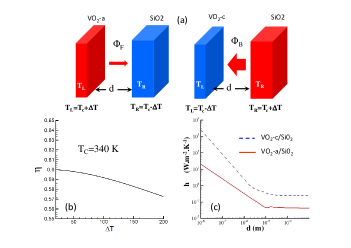
Figure 2: (a) Phase-change radiative thermal diode. In the forward scenario (top-left) a IMT phase-change material (here VO₂) is in its metallic state (VO₂-a) at a temperature higher than $T_{\text{c}}$. In the backward scenario (top right), the phase-change material is in its insulating state (VO₂-c). (b) Rectification coefficient in far-field regime of a VO₂/SiO₂ system with respect to the temperature difference $\Delta T$. The phase transition of VO₂ occurs at $T_{\text{c}}=300\,{\rm K}$. (c) Heat transfer coefficent $h$ evaluated at $T=T_{\text{c}}$ for VO₂ is in its metallic or insulating state, respectively. $h$ is plotted with respect to the separation distance $d$.

.

With the above expressions we can determine the heat flux in the forward and backward case for different temperature differences $\Delta T$. The resulting rectification coefficients $\eta$ of the system in Fig. 2(a) are plotted in Figure 2(b) in far-field regime. It decreases monotonously with the temperature difference $\Delta T$ between both samples. For very small temperature differences we see that $\eta\approx 60\%$ illustrating the high rectification efficiency of the phase transition of VO₂. This efficiency is very large given the fact that we use the simplest possible geometrie. This prediction has been recently experimentally verified Ito . This rectification process could probably be futher improved by texturing the medium as suggested in Ref. NefzaouiEtAl2013 .

In order to understand this large difference of the radiative heat flow in forward and backward direction we have plotted in Fig. 3 the spectral heat flux $\varphi(\omega,d\rightarrow\infty)$ defined in Eq. (2) using the transmission coefficient (4) for the forward and backward scenario. We note that when VO₂ is in its metallic phase (forward scenario, $T_{\text{L}}>T_{c}$), the spectral heat flux is broadband and scales approximately like $\propto\omega^{2}$. The same is true when VO₂ is in its insulating phase. The difference is that in the insulating phase the spectral heat flux is generally larger and shows much more structure. This can be understood by the reflectivity of VO₂ which is plotted in Fig. 3(b). In the metallic phase the reflectivity of VO₂ is relatively high as can be expected from a metallic material whereas in the insulating phase the reflectivity is generally much smaller in the shown frequency range. Therefore it follows directly from Kirchhoff’s law that the emissivity of VO₂ in the metallic phase is smaller than in the insulating phase. This asymetry is the key for obtaining a highly efficient phase-change thermal diode. It is interesting to note, that in the spectral region around $10^{14}\,{\rm rad}/{\rm s}$ the reflectivity of VO₂ in its insulating phase can also be relatively large and attain values close or even larger than that in its metallic phase. In this frequency band, the insulating VO₂ is metal-like which means here that the permittivity can be negative. In this regime VO₂ in its insulating phase supports surface polaritons.

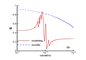
Figure 3: (a) Plot of the spectral heat flux $\varphi_{\text{F}/\text{B}}$ (in far-field regime) introduced in Eq. (2) as a function of frequency for forward direction where VO₂ is in its metallic phase and the reverse situation where VO₂ is in its insulating phase. In addition, we have plotted $\varphi=\frac{\omega^{2}}{\pi^{2}c^{3}}\frac{c}{4}$ for the case that both materials are perfect black bodies, i.e. $\mathcal{T}_{j,\text{R}/\text{B}}=1$ for all propagating modes. (b) Plot of the reflectivity $R$ of VO₂ in its insulating and metallic phase for normal incidence as function of frequency.

In near-field regime that is to say when the separation distance between the VO₂ and SiO₂ samples is smaller than the thermal wavelength, the ’diodicity’ of system becomes even better as we see on Figure 2(c) by comparing the heat transfer coefficients

$$h_{\text{F}/\text{B}}=\frac{\partial\Phi_{\text{F}/\text{B}}}{\partial T}\biggr{|}_{T=T_{\text{c}}}$$ (13)

for the forward and backward scenarios as a function of the separation distance $d$ when temperature is equal to $T_{c}$. We observe a very large thermal contrast of about two orders of magnitude in the near field against about a factor 5 in the far field. In order to understand the physics involved in this spectacular increasement, we have plotted in Fig. 4 the the transmission coefficients for both phases of VO₂ in the ($\omega,k$) plane at a given separation distance in near-field regime. For insulating VO₂ we see in Fig. 4(a) that this coefficient is close to one far beyond the light line $\kappa=\omega/c$. In this region the contribution of the surface phonon polaritons of VO₂ which couple to the surface polaritons of SiO₂ can be observed (see van Zwol1 for a detailed discussion). As the coupling is rather efficient in this region, the heat transfer is large. On the other hand, when VO₂ is metallic we obtain the transmission coefficient shown in Fig. 4(b), the surface phonon-polariton contribution disappears and as a consequence the heat transfer is small. A detailed discussion of the efficiency of rectification in such diode as a function of the thickness of the slabs can be found in Ref. LipingWang . Also, based on a similar idea, a contactless thermal switch has been recently suggested Switch .

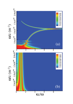
Figure 4: (a) Transmission coefficient $\mathcal{T}_{\text{p},\text{R}/\text{B}}$ (p polarization) between two insulating VO₂ surfaces and (b) between two metallic VO₂ surfaces. Both graphs were obtained for a separation distance $d=500\,{\rm nm}$. The spectral character of thermal transfer changes radically across the phase transition

.

III Photonic thermal transistor

The thermal diode allows the heat flow to propagate preferentially in one direction, but such a device does not allow for switching, modulating or even amplifying the flux exchanged between a hot and a cold body. However, in recent years, physicists have begun to design and test thermal transistors with some success BaowenLiEtAl2012 . In this paragraph we discuss the possibility to design a radiative thermal analog of electronic transistors as depicted in Fig. 5(a). The classical field-effect transistor (FET) which is composed by three basic elements, the drain, the source, and the gate, is basically used to control the flux of electrons (the current) exchanged in the channel between the drain and the source by changing the voltage bias applied on the gate. The physical diameter of this channel is fixed, but its effective electrical diameter can be varied by the application of a voltage on the gate. A small change in this voltage can cause a large variation in the current from the source to the drain.

Recently, a thermal counterpart of the FET has been proposed PBA_PRL2014 to control the near-field radiative heat exchanges between two bodies. This near-field thermal transistor (NFTT) is depicted in Fig. 5(b) and basically consists of a source and the drain, labeled by the indices S and D, which are maintained at temperatures $T_{\text{S}}$ and $T_{\text{D}}$ using thermostats where $T_{\text{S}}>T_{\text{D}}$ so that we have a net heat flux from the source towards the drain. A thin layer of IMT material labeled by G of width $\delta$ is placed between the source and the drain at a distance $d$ from both media and functions as the gate. This IMT material is able, as we have seen before, to qualitatively and quantitatively change its optical properties through a small change of its temperature around a critical temperature $T_{\text{c}}$. As in the previous paragraph we describe here the operating modes of radiative transistor using VO₂ as such IMT material. The choice of IMT depends on the operating temperature of the transistor. If the transistor should operate around $T=500\,{\rm K}$ then VO₂ could be replaced by LaCoO₃, for instance. For the source and the drain we use again SiO₂. Hence we have in principle two oppositely biased diodes as discussed in the previous section which are connected in series so that the NFTT (for which we had a field-effect transistor in mind) can also be regarded as a bipolar transistor.

Without external excitation, the system will reach its steady state for which the net flux $\Phi_{\text{G}}$ received by the intermediate medium, the gate, is zero by heating or cooling the gate until it reaches its steady state or equilibrium temperature $T_{\text{G}}^{\rm eq}$. In this case the gate temperature $T_{\text{G}}$ is set by the temperature of the surrounding media, i.e. the drain and the source. When a certain amount of heat is added to or removed from the gate for example by applying a voltage difference through a couple of electrodes as illustrated in Fig. 5(b) or by extracting heat using Peltier elements, its temperature can be either increased or reduced around its equilibrium temperature $T_{G}^{eq}$. This external action on the gate allows to tailor the heat flux $\Phi_{\text{S}}$ between the source and the gate and the heat flux $\Phi_{\text{D}}$ between the gate and the drain.

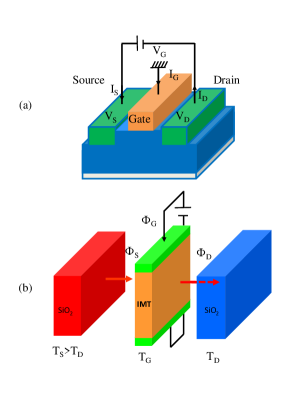
Figure 5: (a) A classical field-effect transistor is a device with three terminals, the source (S), the gate (G), and the drain (D). The gate is used to actively control (by applying a voltage $V$ bias on it) the apparent electric conductivity of the channel between the source and the drain. (b) A radiative thermal transistor. A membrane of an IMT material (VO₂) acts as the gate between two silica (SiO₂) thermal reservoirs (source and drain). The temperature ($T_{\text{G}}$) of the gate is in steady state between the temperatures of the source and drain ($T_{\text{S}}$ and $T_{\text{D}}$). $\Phi_{\text{D}}$ and $\Phi_{\text{S}}$ are the radiative heat fluxes received by the drain and emitted by the source, respectively.

.

In order to see, if this system can be operated as a thermal transistor we need first to determine the radiative heat flux in this system, which is a little bit more complex then the system studied for the radiative thermal diode. In a three-body system the radiative flux received by the drain takes the form Messina

$$\Phi_{\text{D}}=\int_{0}^{\infty}\!\frac{d\omega}{2\pi}\,\phi_{\text{D}}(\omega,d),$$ (14)

where the spectral heat flux is given by

$$\begin{split}\phi_{\text{D}}&=\sum_{j=\{\rm s,p\}}\int\!\frac{{\rm d}^{2}\bm{\kappa}}{(2\pi)^{2}}\,\bigl{[}\Theta_{\text{S}\text{G}}(\omega)\mathcal{T}^{\text{S}/\text{G}}_{j}(\omega,\bm{\kappa};d)\\ &\quad+\Theta_{\rm GD}(\omega)\mathcal{T}^{\text{G}/\text{D}}_{j}(\omega,\bm{\kappa};d)\bigr{]}.\end{split}$$ (15)

This time $\mathcal{T}^{\text{S}/\text{G}}_{j}$ and $\mathcal{T}^{\text{G}/\text{D}}_{j}$ denote the transmission coefficients of each mode $(\omega,\bm{\kappa})$ between the source and the gate and between the gate and the drain for both polarization states $j=\text{s},\text{p}$. In the above relation $\Theta_{ij}$ denotes the difference of functions $\Theta(\omega,T_{i})$ and $\Theta(\omega,T_{j})$. According to the N-body near-field heat transfer theory presented in Ref. Messina , the transmission coefficients $\mathcal{T}^{\text{S}/\text{G}}_{j}$ and $\mathcal{T}^{\text{G}/\text{D}}_{j}$ of the energy carried by each mode written in terms of optical reflection coefficients $\rho_{E,j}$ ($\text{E}=\text{S},\text{D},\text{G}$) and transmission coefficients $\tau_{E,j}$ of each basic element of the system and in terms of reflection coefficients $\rho_{EF,j}$ ($E=\text{S},\text{D},\text{G}$ and $F=\text{S},\text{D},\text{G}$) of couples of elementary elements Messina

$$\begin{split}&\mathcal{T}^{\text{S}/\text{G}}_{j}(\omega,\bm{\kappa},d)\\ &=\frac{4\mid\tau_{\text{G},j}\mid^{2}{\rm Im}(\rho_{\text{S},j}){\rm Im}(\rho_{D,j})\text{e}^{-4\gamma d}}{\mid 1-\rho_{\text{S}\text{G},j}\rho_{\text{D},j}\text{e}^{-2\gamma d}\mid^{2}\mid 1-\rho_{\text{S},j}\rho_{\text{G},j}\text{e}^{-2\gamma d}\mid^{2}},\\ &\mathcal{T}^{\text{G}/\text{D}}_{j}(\omega,\bm{\kappa},d)=\frac{4{\rm Im}(\rho_{\text{S}\text{G},j}){\rm Im}(\rho_{\text{D},j})\text{e}^{-2\gamma d}}{\mid 1-\rho_{\text{S}\text{G},j}\rho_{\text{D},j}\text{e}^{-2\gamma d}\mid^{2}}\end{split}$$ (16)

introducing the imaginary part of the wavevector normal to the surfaces in the multilayer structure $\gamma={\rm Im}(k_{z0})$. Similarly the heat flux from the source towards the gate reads

$$\begin{split}\phi_{\text{S}}&=\sum_{j=\{\rm s,p\}}\int\!\frac{{\rm d}^{2}\bm{\kappa}}{(2\pi)^{2}}\,\bigl{[}\Theta_{\text{D}\text{G}}(\omega)\mathcal{T}^{\text{D}/\text{G}}_{j}(\omega,\bm{\kappa};d)\\ &\quad+\Theta_{\text{G}\text{S}}(\omega)\mathcal{T}^{\text{G}/\text{S}}_{j}(\omega,\bm{\kappa};d)\bigr{]}\end{split}$$ (17)

where the transmission coefficients are analog to those defined in Eq. (16) and can be obtained making the substitution $\text{S}\leftrightarrow\text{D}$. At steady state, the net heat flux received/emitted by the gate which is just given by the heat flux from the source to the gate minus the heat flux from the gate to the drain vanishes, i.e. $\Phi_{\text{S}}=\Phi_{\text{D}}$ or

$$\Phi_{\text{G}}=\Phi_{\text{S}}-\Phi_{\text{D}}=0.$$ (18)

This relation allows us to identify the gate equilibrium temperature $T^{\rm eq}_{\text{G}}$ (which is not necessary unique because of the presence of bistability mechanisms PBA_PRL2014 ) for given temperatures $T_{\text{S}}$ and $T_{\text{D}}$. Note that out of steady state, the heat flux received/emitted by the gate is $\Phi_{\text{G}}=\Phi_{\text{S}}-\Phi_{\text{D}}\neq 0$. If $\Phi_{\text{G}}<0$ ($\Phi_{\text{G}}>0$) an external flux is added to (removed from) the gate by heating (cooling).

To illustrate the different operating modes of the NFTT we consider now our system of a silica source and a silica drain with a VO₂ gate in between. We set $T_{\text{S}}=360\,{\rm K}$ and $T_{D}=300\,{\rm K}$ and choose a separation distance between the source and the gate and between the gate and the drain of $d=100\,{\rm nm}$. The thickness of the gate layer is set to $\delta=50\,{\rm nm}$. Therefore, the NFTT operates in the near-field regime (of course, it would also work in the far-field regime). The equilibrium temperature of the gate is obtained by solving the transcendental equation (18). Here we find $T^{\rm eq}_{G}=332\,{\rm K}$ which is close to the critical temperature $T_{\text{c}}\approx 340\,{\rm K}$ of VO₂ which means that in the steady-state situation the gate is in its insulating phase. In this situation the surface modes of the gate and the source and the drain can couple which results in large heat fluxes $\Phi_{\text{S}}$ and $\Phi_{\text{D}}$. On the other hand, when the temperature of the gate is increased by external heating to values larger than $T_{\text{c}}$ then VO₂ undergoes a phase transition towards its metallic phase. In this phase we can expect from the discussion of the diode that the coupling between the gate and the source and the drain will be much less efficient so that $\Phi_{\text{S}}$ and $\Phi_{\text{D}}$ can be expected to drop. In the transition regime around $T_{\text{c}}$ we model the effective permittivity $\epsilon^{\rm eff}_{\parallel/\perp}$ of VO₂ parallel and perpendicular to the optical axis by a simple effective medium theory (EMT) ansatz

$$\epsilon^{\rm eff}_{\parallel/\perp}=f\epsilon^{\rm m}_{\parallel/\perp}+(1-f)\epsilon^{\rm d}_{\parallel/\perp}$$ (19)

and by a Bruggemann model (BM)

$$f\frac{\epsilon^{\rm d}_{\parallel/\perp}-\epsilon^{\rm eff}_{\parallel/\perp}}{\epsilon^{\rm d}_{\parallel/\perp}+2\epsilon^{\rm eff}_{\parallel/\perp}}+(1-f)\frac{\epsilon^{\rm m}_{\parallel/\perp}-\epsilon^{\rm eff}_{\parallel/\perp}}{\epsilon^{\rm m}_{\parallel/\perp}+2\epsilon^{\rm eff}_{\parallel/\perp}}=0$$ (20)

which is inspired by the measurements and modelling in Ref. Mott . Here $\epsilon^{\rm d}_{\parallel/\perp}$ is the permittivity of VO₂ in its insulating phase and $\epsilon^{\rm m}_{\parallel/\perp}$ is the permittivity of VO₂ in its metallic phase. The filling fraction $f$ is chosen to be linear in $T_{\text{G}}$ such that the phase transition starts at $T_{\text{G}}=341.2\,{\rm K}$ and ends at $T_{\text{G}}=345.2\,{\rm K}$. Of course, this model can be improved by using measurements of the permittivities in the transition region.

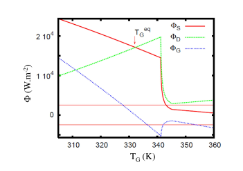
Figure 6: Heat fluxes inside the near-field thermal transistor using a VO₂ gate of thickness $\delta=50\,{\rm nm}$ located at a distance $d=100\,{\rm nm}$ between two massive silica samples maintained at temperatures $T_{\text{S}}=360\,{\rm K}$ and $T_{\text{D}}=300\,{\rm K}$. By changing the flux $\Phi_{\text{G}}$ supplied to the gate the temperature $T_{\text{G}}$ is changed which allows to operate the NFTT as a thermal switch, a thermal modulator and a thermal amplifier.

.

Using the above parameters together with the EMT model for the permittivity of VO₂ we find the resulting heat fluxes $\Phi_{\text{S}}$, $\Phi_{\text{D}}$ and $\Phi_{\text{G}}$ as shown in Fig. 6. These results illustrate that the NFTT can operate as (i) a thermal switch, (ii) a thermal modulator or (iii) a thermal amplifier. But let us discuss these functions of the NFTT in more detail:

(i)Thermal switching :

An increase of $T_{\text{G}}$ by about 10 degrees starting from $T_{\text{G}}=T_{\text{G}}^{\rm eq}$ leads, as clearly shown in Fig. 7, to a reduction of heat flux received by the drain and lost by the source by about one order of magnitude. That means the NFTT can be used in two operating modes where $T_{\text{G}}$ is slightly below or above the critical temperature $T_{\text{c}}$, where in the case $T_{\text{G}}<T_{\text{c}}$ we have a large heat flux to the drain which can be assigned as the ”on” mode and for $T_{\text{G}}>T_{\text{c}}$ the heat flux towards the drain drops by one order of magnitude which can be assigned as the ”off” mode. The thermal inertia of the gate as well as its phase transition delay defines the timescale at which the switch can operate. Usually the thermal inertia limits the speed to some microseconds Tschikin ; Dyakov2 .

(ii)Thermal modulation:

Over a relatively broad temperature range around $T^{\rm eq}_{G}$ (strip between the vertical lines in Fig. 6) the heat current $\Phi_{\text{G}}$ from or towards the gate remains relatively small compared to the $\Phi_{\text{S}}$ and $\Phi_{\text{G}}$ (i.e. $\Phi_{S}\approx\Phi_{D}$). Within this temperature range the flux received by the drain or lost by the source can be modulated. A much larger modulation of fluxes can be achieved with the NFTT when setting $T_{\text{S}}$ and $T_{\text{D}}$ such that $T^{\rm eq}_{\text{G}}\approx T_{\text{c}}$. Then the flux can be modulated over one order of magnitude by a small temperature change of $T_{\text{G}}$.

(iii)Thermal amplification:

The most important feature for a transistor is its ability to amplify the current or electron flux towards the drain. In the region of phase transition around $T_{\text{c}}$ we see in Fig. 6 that an increase of $T_{\text{G}}$ leads to a drastic reduction of flux received by the drain. As described by Kats et al. in Ref.Kats this behavior can be associated (in far-field) to a reduction of the thermal emission. This corresponds to a negative differential thermal conductance (NDTC) as described for SiC in Ref. Fan and illustrated for our configuration in Fig. 8. Having a NDTC is the key for having an amplification which is defined as (see for example Ref. Casati1 )

$$\alpha\equiv\biggl{|}\frac{\partial\Phi_{\text{D}}}{\partial\Phi_{\text{G}}}\biggl{|}=\frac{1}{\biggl{|}1-\frac{\Phi_{\text{S}}^{\prime}}{\Phi_{\text{D}}^{\prime}}\biggr{|}}$$ (21)

where

$$\Phi_{\text{S}/\text{D}}^{\prime}\equiv\frac{\partial\Phi_{\text{S}/\text{D}}}{\partial T_{\text{G}}}.$$ (22)

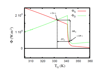
Figure 7: Switching mode of radiative transistor: When the gate temperature $T_{\text{G}}$ is slightly increased above its critical temperature $T_{\text{c}}$ the heat flux $\Phi_{D}$ received by the drain falls from a relatively large value, the so-called ”on” mode, to a value which is about one order of magnitude smaller, the so-called ”off” mode.

It can be easily seen from Fig. 6 that $\alpha=1/2$ for $T_{\text{G}}$ outside the phase transition region where the material properties of VO₂ are more or less independent of $T_{\text{G}}$, since $\Phi_{S}^{\prime}=-\Phi_{D}^{\prime}$ in this region. On the other hand, inside the transition region of VO₂ that means for temperatures around $T_{\text{c}}$ the material properties of VO₂ change drastically showing a NDTC which leads to an amplification of about 4 regardless of using the EMT or BM for modelling the permittivity in the transition region PBA_PRL2014 .

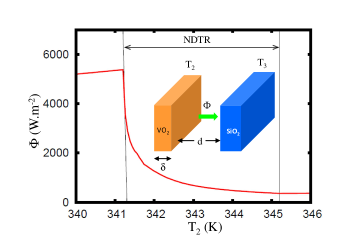
Figure 8: Illustration of the negative differential conductance (NDTC) between a VO₂ layer $\delta=50\,{\rm nm}$ thick and a massive SiO₂ sample separated by a vacuum gap of $d=100\,{\rm nm}$. The flux $\Phi$ exchanged between both media is in the phase-transition region $T_{2}\in[341.2\,{\rm K},345.2\,{\rm K}]$ a decreasing function of the VO₂ temperature $T_{2}$. Outside this transition region the flux $\Phi$ increases with temperature. Here the temperature of SiO₂ is fixed to $300\,{\rm K}$.

Figure 9: Efficiency of the mode coupling in ($\omega,\bm{\kappa}$)-space for a SiO₂-VO₂-SiO₂ system ($\delta=50\,{\rm nm}$ and $d=100\,{\rm nm}$). (a) $\mathcal{T}^{\text{S}/\text{G}}_{\text{p}}$ and (b) $\mathcal{T}^{\text{G}/\text{D}}_{\text{p}}$ with VO₂ in its insulating state. (c) $\mathcal{T}^{\text{S}/\text{G}}_{\text{p}}$ and (d) $\mathcal{T}^{\text{G}/\text{D}}_{\text{p}}$ with VO₂ in its metallic state. Wien’s frequency (where the heat transfer is maximal) at $T=340\,{\rm K}$ is $\omega_{\rm Wien}\approx 1.3\times 10^{14}\,{\rm rad/s}$.

To explain the strong variations of heat flux observed inside our NFTT, let us examine hereafter the transmission coefficients (only p polarisation) of the energy carried by the modes $(\omega,\bm{\kappa})$ through such a three-body system which are plotted in Fig. 9. When the gate is in its insulating state, $\mathcal{T}^{\text{S}/\text{G}}_{\text{p}}$, which represents the exchange between the source and the drain mediated by the presence of the gate [see Fig. 9(a)], and $\mathcal{T}^{\text{G}/\text{D}}_{\text{p}}$, which corresponds to the exchange between the couple source-gate treated as a unique body and the drain [see Fig. 9(b)] shows an efficient coupling of modes between the different blocks of the system around the resonance frequencies $\omega_{\rm SPP1}\approx 1\times 10^{14}\,{\rm rad/s}$ and $\omega_{\rm SPP2}\approx 2\times 10^{14}\,{\rm rad/s}$ of surface waves (surfaces phonon-polaritons) supported by both the source and the drain. Below $T_{\text{c}}$ all parts of the system support surface waves in the same frequency range close to the thermal peak frequency $\omega_{\rm Wien}\approx 1.3\times 10^{14}\,{\rm rad/s}$. The anti-crossing curves which appear in Fig. 9(a) and (b) result from the strong coupling of silica surface phonon-polaritons (SPPs) and the surface waves (symmetric and antisymmetric ones) supported by the thin VO₂ layer. Beyond $T_{\text{c}}$ the gate becomes metallic and it does not support surface waves anymore. In this case $\mathcal{T}^{\text{S}/\text{G}}_{\text{p}}$ [see Fig. 9(c)] vanishes owing to the field screening by the gate. Moreover, as is clearly shown in Fig. 9(d), the coupling of modes between the source-gate and the drain at the frequency of surface waves is less efficient for the large parallel values of $\kappa$ reducing so the transfer of heat towards the drain, i.e. the number of participating modes decreases BiehsEtAl2010 ; JoulainPBA2010 .

IV Volatile radiative memory

Manipulating radiative heat fluxes is only a first step towards the development of a contactless technology for the thermal management of systems at tha nano and macroscale. In this last section, we examine the possibility to store information or energy for arbitrary long time using thermal photons by introducing the concept of a radiative thermal memory. The concept of thermal memory is closely related to the thermal bistability of a system that means to the presence of at least two temperature set’s which lead to a steady state BaowenLi3 .

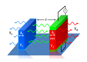
Figure 10: Sketch of a radiative thermal memory. A membrane made of an IMT material is placed at a distance $d$ from a dielectric layer. The system is surrounded by two thermal baths at different temperatures $T_{\rm L}$ and $T_{\rm R}$. The temperature $T_{2}$ can be increased or reduced either by Joule heating by applying a voltage difference through a couple of electrodes or by using Peltier elements.

To illustrate this, let us consider a concrete system as depicted in Fig. 10 composed by two parallel homogeneous membranes made of VO₂ and SiO₂. These slabs have finite thicknesses $\delta_{1}$ and $\delta_{2}$ and are separated by a vacuum gap of distance $d$. The left (right) membrane is in contact with a thermal bath having a temperature $T_{\rm L}$ ($T_{\rm R}$), where $T_{\rm L}\neq T_{\rm R}$. In a practical point of view, the field radiated by these baths can be produced by two external blackbodies. The membranes themselves interact on the one hand through the intracavity fields and on the other with the thermal baths which can be thought to be produced by external media. In that sense, the system is driven by many-body interactions in contrast to the diode in section II which is only a two-body system.

The heat flux across any plane $z=\bar{z}$ parallel to the interacting surfaces can again be evaluated using Rytov’s fluctuational electrodynamics Rytov ; Polder . For the sake of simplicity we assume that the separation distance $d$ is large enough compared to the thermal wavelengths [i.e. $d\gg\max(\lambda_{T_{i}}=c\hbar/(k_{\text{B}}T_{i})$, $i=1,2,{\rm L},{\rm R}$ ] so that near-field heat exchanges can be neglected (a memory using the near-field effect was proposed quite resently in Ref. DyakovMemory ). In this case we obtain

$$\begin{split}\varphi(\bar{z})=2\epsilon_{0}c^{2}\!\!\sum\limits_{\underset{\phi=\left\{+,-\right\}}{j=s,p}}\int_{0}^{\infty}\!\!\frac{d\omega}{2\pi}\int\!\!\!\frac{{\rm d}^{2}\bm{\kappa}}{(2\pi)^{2}}\frac{\phi k_{z0}}{\omega}\mathfrak{C}_{j}^{\phi,\phi}(\omega,\bm{\kappa}),\end{split}$$ (23)

where the field correlators Messina3

$$\mathfrak{C}_{j}^{\phi,\phi^{\prime}}(\omega,\bm{\kappa})=\frac{1}{2}\langle[E_{j}^{\phi}(\omega,\bm{\kappa})E_{j}^{\phi^{\prime}\dagger}(\omega,\bm{\kappa})+E_{j}^{\phi^{\prime}\dagger}(\omega,\bm{\kappa})E_{j}^{\phi}(\omega,\bm{\kappa})]\rangle$$ (24)

of local field amplitudes in polarization $j$ can be expressed (see the supplemental material in Slava for details) in terms of reflection and transmission operators $\mathfrak{R}_{i}^{\pm}$ and $\mathfrak{T}_{i}^{\pm}$ of the layer $i$ toward the right ($+$) and the left ($-$), as

$$\begin{split}\mathfrak{C}_{1}^{+,+}=\mathcal{S}(T_{1})(1-\mid\mathfrak{R}_{1}^{+}\mid^{2}-\mid\mathfrak{T}_{1}^{+}\mid^{2}),\\ \mathfrak{C}_{2}^{-,-}=\mathcal{S}(T_{2})(1-\mid\mathfrak{R}_{2}^{-}\mid^{2}-\mid\mathfrak{T}_{2}^{-}\mid^{2}),\\ \mathfrak{C}_{L}^{+,+}=\mathcal{S}(T_{L}),\;\;\;\;\;\;\;\;\;\;\;\;\;\;\;\;\;\;\;\;\;\;\;\;\;\;\;\;\;\;\;\;\;\;\\ \mathfrak{C}_{R}^{-,-}=\mathcal{S}(T_{R}),\;\;\;\;\;\;\;\;\;\;\;\;\;\;\;\;\;\;\;\;\;\;\;\;\;\;\;\;\;\;\;\;\;\;\\ \end{split}$$ (25)

with

$$\mathcal{S}(T)=\pi\frac{\omega}{\epsilon_{0}c^{2}}\Theta(\omega,T){\rm Re}\biggl{(}\frac{1}{k_{z}}\biggr{)}.$$ (26)

Here $k_{z}$ denotes the normal component of wave vector in the medium of consideration. Using expression (23) we can calculate the net flux $\Phi_{1}=\varphi(0)-\varphi(-\delta_{1})$ [resp. $\Phi_{2}=\varphi(d+\delta_{2})-\varphi(d)$] received by the first (resp. second) membrane.

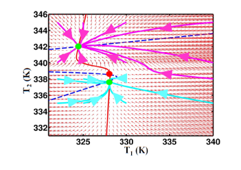
Figure 11: Trajectories of temperatures (i.e. phase portrait) for different initial conditions in the plane ($T_{1},T_{2}$) in a two membrane SiO₂/VO₂ system with $\delta_{1}=\delta_{2}=1\,\mu{\rm m}$. The blue dashed and red solid lines represent the local equilibrium conditions $\Phi_{1}=0$ and $\Phi_{2}=0$ of each membrane. The green (red) points denote the stable (unstable) global steady-state temperatures, $(T_{1}^{(1)},T_{2}^{(1)})=(328.03\,{\rm K},337.77\,{\rm K})$, $(T_{1}^{(2)},T_{2}^{(2)})=(328.06\,{\rm K},338.51\,{\rm K})$, and $(T_{1}^{(3)},T_{2}^{(3)})=(324.45\,{\rm K},341.97\,{\rm K})$. The red arrows represents the vector field $\bm{\Phi}$. The temperature of thermal reservoirs are $T_{\rm L}=320\,{\rm K}$ and $T_{\rm R}=358\,{\rm K}$.

The time evolution of temperatures $T_{1}$ and $T_{2}$ of the two membranes are solution of the following nonlinear coupled system of differential equations

$$\partial_{t}\mathbf{T}=\bm{\Phi}+\mathbf{Q}$$ (27)

where we have introduced the vectors $\mathbf{T}\equiv\bigl{(}T_{1}(t),T_{2}(t)\bigr{)}^{\text{t}}$, $\bm{\Phi}\equiv\bigl{(}\Phi_{1}(T_{1},T_{2})/I_{1},\Phi_{2}(T_{1},T_{2})/I_{2}\bigr{)}^{\text{t}}$, and $\mathbf{Q}\equiv(Q_{1}\delta_{1}/I_{1},Q_{2}\delta_{2}/I_{2})^{\text{t}}$. Here $Q_{i}$ ($i=1,2$) is the power per unit volume which can be added to or extracted from both membranes by applying a voltage difference through a couple of electrodes as illustrated in Fig. 10 or by using Peltier elements. Furthermore, we have introduced the thermal inertia of both membranes as $I_{i}\equiv C_{i}\rho_{i}\delta_{i}$, where $C_{i}$ and $\rho_{i}$ are the heat capacity and the mass density of each material. By writing down this set of equations we have neglected any temperature variation inside the membranes which is a very good approximation given that the conductivity inside the membranes is much larger than between the membranes. When assuming that no energy is directly added to or removed from the membranes, then $\mathbf{Q}=\mathbf{0}$. In this case, the steady-state solution is given by $\bm{\Phi}=\mathbf{0}$. Hence $\Phi_{1}$ and $\Phi_{2}$ vanish for the same couple of temperatures $(T_{1}^{({\rm st-st})},T_{2}^{(\rm st-st)})$. Considering for an instant membrane 2 only, then the existence of two equilibrium temperatures where the net flux vanishes ($\Phi_{2}=0$) implies that $\Phi_{2}$ must have a maximum or a minimum between these two temperatures. Hence, this requires a negative differential conductive behavior for this membrane which was shown in the previous section for VO₂. For the whole system it is therefore a precondition to have at least one membrane which exihibits negative differential conductive behavior in order to have two couples $(T_{1}^{({\rm st-st})},T_{2}^{(\rm st-st)})$ of steady-state temperatures.

In Fig. 11, we show the time evolution of the SiO₂-VO₂ system without external excitation (i.e. $\mathbf{Q}=\mathbf{0}$) when the thermal inertia $I_{i}$ of both membranes are comparable (i.e. $\delta_{1}\thickapprox\delta_{2}$) or very different (i.e. $\delta_{1}\gg\delta_{2}$). The trajectories (the thick pink and turquois lines) are obtained by solving Eq. (28) using a Runge-Kutta method with adaptative time steps choosing different initial conditions. In this figure, the dashed blue (solid red) line represents the local equilibrium temperatures for the first (second) membrane that is the set of temperatures couples ($T_{1},T_{2}$) which satisfy the condition $\Phi_{1}(T_{1},T_{2})=0$ [$\Phi_{2}(T_{1},T_{2})=0$]. The intersection of these two lines define the global steady-state temperatures of the system where $\bm{\Phi}=\mathbf{0}$. Only two of three equilibrium points $\mathbf{T}\equiv(T^{eq}_{1},T^{eq}_{2})^{t}$ that appear in Fig. 11 are stable. These points can be identified by applying a small perturbation $\delta\mathbf{T}\equiv(\delta T_{1}(t),\delta T_{2}(t))^{t}$ on them and look at the relaxation process. Then, the time evolution of each perturbation is driven by the following equation

$$\partial_{t}(\delta\mathbf{T})=\mathbf{J}\cdot\delta\mathbf{T},$$ (28)

where

$$\mathbf{J}=\left(\begin{array}[]{cc}\frac{1}{I_{1}}\frac{\partial\Phi_{1}}{\partial T_{1}}&\frac{1}{I_{1}}\frac{\partial\Phi_{1}}{\partial T_{2}}\\ \frac{1}{I_{2}}\frac{\partial\Phi_{2}}{\partial T_{1}}&\frac{1}{I_{2}}\frac{\partial\Phi_{2}}{\partial T_{2}}\end{array}\right)$$ (29)

is the Jacobian matrix associated to the dynamical system. Its solution reads

$$\delta\mathbf{T}(t)=\delta\mathbf{T}(0)\exp(\mathbf{J}t).$$ (30)

Hence, the eigenvalues $\lambda_{i}$ of $\mathbf{J}$ allow to determine the stability of thermal state. In a two membrane SiO₂-VO₂ system with $\delta_{1}=\delta_{2}=1\,\mu{\rm m}$ and with reservoirs temperatures $T_{\rm L}=320\,{\rm K}$ and $T_{\rm R}=358\,{\rm K}$ the stability analysis leads to

$T^{\rm eq}_{1}(K)$	$T^{\rm eq}_{2}(K)$	$\lambda_{1}$	$\lambda_{2}$	stability
328.03	337.77	-2.58	-1.37	stable
328.06	338.51	-2.51	3.69	unstable
324.45	341.97	-2.31	-4.70	stable

where we have used the volumetric densities and the heat capacities $\rho_{1}=2180\,{\rm kg}{\rm m}^{-3}$, $\rho_{2}=4339{\rm kg}{\rm m}^{-3}$, $C_{1}=750{\rm J}{\rm kg}^{-1}{\rm K}^{-1}$ and $C_{2}=690{\rm J}{\rm kg}^{-1}{\rm K}^{-1}$.

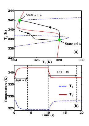
Figure 12: (a) Hystereis of the VO₂ membrane temperature during a transition between the thermal states ”0” and ”1” inside a two membrane SiO₂/VO₂ system with $\delta_{1}=\delta_{2}=1\,\mu{\rm m}$. The volumic powers supplied and extracted from the VO₂ layer during a time interval $\Delta t_{1}=0.4\,{\rm s}$ and $\Delta t_{2}=1.5\,{\rm s}$ are $Q_{2}=10^{-2}\,{\rm W}{\rm mm}^{-3}$ and $Q_{2}=-2.5\times 10^{-2}{\rm W}{\rm mm}^{-3}$, respectively. The writing time of state ”1” (”0”) from the state ”0” (”1”) is $\Delta t(0\rightarrow 1)=4\,{\rm s}$ ($\Delta t(1\rightarrow 0)=8\,{\rm s}$). (b) Time evolution of temperature $T_{1}(t)$ and $T_{2}(t)$ of SiO₂ and VO₂ membranes. The thermal states ”0” and ”1” can be maintained for arbitrary long time provided that the thermostats ($T_{L}=320\,{\rm K}$ and $T_{R}=358\,{\rm K}$) remain switched on.

From this result, it becomes apparent that it is possible to use the SiO₂-VO₂ system as a thermal memory Slava . Indeed, the two stable equilibrium temperatures can be viewed as two thermal states ”0” and ”1” of the system. To switch from one thermal state to the other, we need to add or extract power from the system. In the following we describe this writing-reading procedure. To this end, we consider the SiO₂-VO₂ system made with membranes of equal thicknesses $\delta_{1}=\delta_{2}=1\,\mu{\rm m}$ which are coupled to two reservoirs of temperatures $T_{\text{L}}=320\,{\rm K}$ and $T_{\text{R}}=358\,{\rm K}$. Let us define ”0” as the thermal state at the temperature $T_{2}=\min(T^{(1)}_{2},T^{(3)}_{2})$. To make the transition towards the thermal state ”1” the VO₂ membrane must be heated.

Step 1 (transition from the state ”0” to the state ”1”): A volumic power $Q_{2}=10^{-2}\,{\rm W}{\rm mm}^{-3}$ is added to this membrane during a time interval $\Delta t_{1}\thickapprox 0.4\,{\rm s}$ to reach a region in the plane ($T_{1},T_{2}$) [see Fig. 12(a)] where all trajectories converge naturally (i.e. for $Q_{2}=0$) after some time toward the state ”1”, the overall transition time is $\Delta t(0\rightarrow 1)=4s$ Fig. 12(b)].

Step 2 (maintaining the stored thermal information): Since the state ”1” is a fixed point, the thermal data can be maintained for arbitrary long time provided that the thermal reservoirs are switched on. This corresponds basically to the concept of volatile memory in electronics.

Step 3 (transition from the state ”1” to the state ”0”): Finally, a volumic power $Q_{2}=-2.5\times 10^{-2}\,{\rm W}{\rm mm}^{-3}$ is extracted from the VO₂ membrane during a time interval $\Delta t_{2}\thickapprox 1.5\,{\rm s}$ to reach a region [below $T_{2}=338\,{\rm K}$ in Fig. 12(a)] of natural convergence to the state ”0” . In this case the transition time becomes $\Delta t(1\rightarrow 0)=8\,{\rm s}$. Compared with its heating, the cooling of VO₂ does not follow the same trajectory [see Fig. 12(a)] outlining the hysteresis of the system which accompanies its bistable behavior. To read out the thermal state of the system a classical electronic thermometer based on the thermo dependance of the electric resistivity of membranes can be used.

V Conclusion

In this paper we have summarized the very recent advances made in optics to manipulate and store the thermal energy with contactless devices. We have demonstrated the feasability for contactless thermal analogs of diodes, transistors and volatile memories. These devices allow for contactless management of heat flows at macroscale and at subwavelength scales. These results pave the way for a novel technology of thermal management. It also suggests the possibility to develop contactless thermal analogs of electronic devices such as thermal logic gates for processing information by utilizing thermal photons rather than electrons. They also could find broad applications in MEMS/NEMS technologies, to generate mechanical work by using microresonators coupled to a transistor as well as in energy storage technology to store and release heat upon request.

- (1) F. Braun, Annalen der Physik und Chemie, 153, 556 (1874).
- (2) J. Bardeen and W. H. Brattain, Phys. Rev. 74, 230 (1948).
- (3) B. Li and L. Wang and G. Casati, Appl. Phys. Lett. 88, 143501 (2006).
- (4) L. Wang, B. Li, Phys. Rev. Lett. 99, 177208 (2007).
- (5) L. Wang and B. Li, Phys. Rev. Lett. 101, 267203 (2008).
- (6) N. Li, J. Ren, L. Wang G. Zhang, P. Hänggi, and B. Li, Rev. Mod. Phys. 84, 1045 (2012).
- (7) E. Ozbay, Science 311, 5758, 189, (2006).
- (8) H. Caglayan, S.-H. Hong, B. Edwards, C. R. Kagan, and N. Engheta, Phys. Rev. Lett. 11, 073904, (2013).
- (9) P. Ben-Abdallah and S.-A. Biehs, Appl. Phys. Lett. 103, 191907 (2013).
- (10) P. Ben-Abdallah and S.-A. Biehs, Phys.Rev. Lett. 112, 044301 (2014).
- (11) V. Kubytskyi, S.-A. Biehs and P. Ben-Abdallah, Phys. Rev. Lett. 113, 074301 (2014).
- (12) C. Starr, J. Appl. Phys. 7, 15 (1936).
- (13) N. A. Roberts and D. G. Walker, Int. J. thermal Sciences 50, 648 (2011).
- (14) B. Li, L. Wand and G. Casati, Phys.Rev. Lett. 93, 184301 (2004).
- (15) C. W. Chang, Okawa D., Majumdar A., and A. Zettl, Science 314, 1121 (2006).
- (16) D. Segal, Phys. Rev. Lett. 100, 105901 (2008).
- (17) H.-Y. Cao, H. Xiang, and X.-G. Gong, Solid State Commun. 152, 1807–1810 (2012).
- (18) M. J. Martinez-Perez and F. Giazotto, Appl. Phys. Lett. 102, 182602 (2013).
- (19) C. R. Otey, W. T. Lau, and S. Fan, Phys. Rev. Lett. 104, 154301 (2010).
- (20) H. Iizuka and S. Fan, J. Appl. Phys. 112, 024304 (2012).
- (21) L. Zhu, C. R. Otey, and S. Fan, Appl. Phys. Lett. 100, 044104 (2012).
- (22) S. Basu and M. Francoeur, Appl. Phys. Lett. 98, 113106 (2011).
- (23) E. Nefzaoui, J. Drevillon, Y. Ezzahri, and K. Joulain, Applied Optics, 53, 16, 3479 (2014) see also E. Nefzaoui, K. Joulain, J. Drevillon, Y. Ezzahri, Appl. Phys. Lett. 104 , 103905 (2014).
- (24) L. P. Wang and Z.M. Zhang, Nanoscale and Microscale Thermophysical Engineering, 17, 337 (2013).
- (25) J. G. Huang, Q. Li, Z. H. Zheng and Y. M. Xuan, Int. J. Heat and Mass Trans., 67, 575 (2013).
- (26) Z. Chen, C. Wong, S. Lubner, S. Yee, J. Miller, W. Jang, C. Hardin, A. Fong, J. E. Garay and C. Dames, Nature Comm., 5, 5446 (2014).
- (27) L. Zhu, C. R. Otey, and S. Fan, Phys. Rev. B 88, 184301 (2013).
- (28) P. van Zwol, K. Joulain, P. Ben-Abdallah, and J. Chevrier, Phys. Rev. B, 84, 161413(R) (2011).
- (29) M. M. Qazilbash, M. Brehm, B. G. Chae, P.-C. Ho, G. O. Andreev, B. J. Kim, S. J. Yun, A. V. Balatsky, M. B. Maple, F. Keilmann, H. T. Kim, and D. N. Basov, Science 318, 5857, 1750-1753 (2007).
- (30) A. S. Barker, H. W. Verleur, and H. J. Guggenheim, Phys. Rev. Lett. 17, 1286 (1966).
- (31) D. Polder and M. Van Hove, Phys. Rev. B 4, 3303 (1971).
- (32) G. Bimonte, Phys. Rev. A 80, 042102 (2009).
- (33) S.-A. Biehs, E. Rousseau, and J.-J. Greffet, Phys. Rev. Lett. 105, 234301 (2010).
- (34) P. Ben-Abdallah and K. Joulain, Phys. Rev. B 82, 121419(R) (2010).
- (35) S.-A. Biehs, P. Ben-Abdallah, F. S. S. Rosa, K. Joulain, and J.-J. Greffet, Opt. Expr. 19, A1088-A1103 (2011).
- (36) P. Yeh, Optical Waves in Layered Media, (John Wiley & Sons, New Jersey, 2005).
- (37) Y. Yang, S. Basu, and L. Wang, Appl. Phys. Lett. 103, 163101 (2013).
- (38) Y. Yang, S. Basu, and L. Wang, Vacuum Thermal Switch Made of Phase Transition Materials Considering Thin Film and Substrate Effects, J. Quant. Spec. Rad. Trans., 2014. doi:10.1016/j.jqsrt.2014.12.002
- (39) R. Messina, M. Antezza and P. Ben-Abdallah, Phys. Rev. Lett. 109, 244302 (2012).
- (40) M. Kats, R. Blanchard, S. Zhang, P. Genevet, C. Ko, S. Ramanathan and F. Capasso, Phys. Rev. X 3, 041004 (2013).
- (41) Handbook of Optical Constants of Solids, edited by E. Palik (Academic Press, New York, 1998).
- (42) K. Ito, K. Nishikawa, H. Lizuka and H. Toshiyoshi, Appl. Phys. Lett. 105, 253503 (2014).
- (43) M. Tschikin, S.-A. Biehs, P. Ben-Abdallah, F. S. S. Rosa, Eur. Phys. J. B 85, 233 (2012).
- (44) S. A. Dyakov, J. Dai, M. Yan, and M. Qiu, Phys. Rev. B 90, 045414 (2014).
- (45) S.M. Rytov, Y. A. Kravtsov and V. I. Tatarskii, Principles of Statistical Radiophysics, Vol. 3, (Academy of Sciences of USSR, Moscow, 1953).
- (46) D. Polder and M. Van Hove, Phys. Rev. B 4, 3303 (1971).
- (47) S. A. Dyakov, J. Dai, M. Yan, and M. Qiu, arXiv:1408.5831v2.