On the Formation of Elliptical Rings in Disk Galaxies

Abstract

N-body simulations of galactic collisions are employed to investigate the formation of elliptical rings in disk galaxies. The relative inclination between disk and dwarf galaxies is studied with a fine step of five degrees. It is confirmed that the eccentricity of elliptical ring is linearly proportional to the inclination angle. Deriving from the simulational results, an analytic formula which expresses the eccentricity as a function of time and inclination angle is obtained. This formula shall be useful for the interpretations of the observations of ring systems, and therefore reveals the merging histories of galaxies.

Key words: galaxies: interactions; galaxies: stellar content; galaxies: dynamics

1 Introduction

Ring galaxies are galaxies which present a very unusual morphology in that rings are observed as dominating parts of their structures. They could be systems with rings surrounding early-type galaxies, such as the Hoag’s object or polar ring galaxies (Hoag 1950; Wakamatsu 1990). They could also be those systems in that the main disk of spiral galaxies are dominated by a ring centered on a nucleus. This paper focuses on the second type, which is as those presented in the catalog of Madore et al. (2009).

Although the secular processes through the bars might be responsible for some of the ring structures in spiral galaxies, the galactic interactions through collisions or merging are the main picture to describe the formation of ring galaxies. The head-on collisions were first proposed by Lynds & Toomre (1976) to be the mechanism to produce ring galaxies. The analytic model of these kinds of collisions employing the caustic wavefronts of stellar rings was developed in Struck-Marcell (1990) and Struck-Marcell & Lotan (1990). Later, Gerber et al. (1992) studied the formation of empty rings, which are those systems without nuclei such as Arp 147. They produced C-shape structures and found that the remnant nucleus is offset from the center and out of the original plane in their simulations. Moreover, Wong et al. (2006) suggested that a high-speed off-center collision can explain their observational results of NGC 922.

Interestingly, Elmegreen & Elmegreen (2006) showed that some ring galaxies with features of collisional rings have no obvious companions. It is thus unclear whether these ring galaxies could be explained by the collision scenario or not. Motivated by this controversial result, Wu & Jiang (2012) picked up some observed axisymmetric ring galaxies from the catalog of Madore et al. (2009) and demonstrated through N-body simulations that head-on collisions could produce the structures of these axisymmetric rings. They thus claimed that the identified off-center companions around the ring galaxies might not be relevant to the rings. The dwarf galaxy which collided with the disk galaxy along the symmetric axis was already mixed with the center of the disk galaxy and became parts of a nucleus of this ring galaxy.

While these results were presented in IAU Symposium (Wu & Jiang 2011), in addition to our paper Wu & Jiang (2012), there were several recent works, such as Smith et al. (2012), Mapelli & Mayer (2012), and Fiacconi et al. (2012), which also investigated the formation of ring galaxies. Smith et al. (2012) modeled the formation of Auriga’s Wheel ring galaxy using N-body simulations. They proposed that Auriga’s Wheel was formed by the collision of a spiral galaxy and an elliptical galaxy. Mapelli & Mayer (2012) investigated the formation of empty ring galaxies, which were considered as collisional ring galaxies without nuclei inside the ring. Fiacconi et al. (2012) explored parameters of galactic collisions and paid attention to the relation between the star formation rate and different parameters. However, the association between different parameters and the shape of the ring galaxies was not clear.

Indeed, as those observed non-axisymmetric rings shown in Madore et al. (2009), it is confirmed that not only the shape of rings could be elliptical, but also that the nucleus could be offset from the center of rings. These complexities are likely due to the details of the collisional history. The interesting questions would be: what kinds of relative orbits between the dwarf and main disk galaxies could lead to these structures?

In order to answer the above question, the link between the merging processes and the shapes of rings needs to be constructed. Once this link is established, through the observations of ring systems, one can investigate the merging histories of galaxies and therefore constrain the cosmology.

To achieve this goal, we here employ N-body simulations to investigate the formation of ring galaxies through non-axisymmetric collisions. The collisions of two galaxies would be set up by making the initial velocity of the dwarf be inclined from the symmetric axis of the main disk galaxy. To narrow down the parameter space and focus on the inclination angle, the dwarf galaxy is assumed to be moving on a parabolic orbit and directly towards to the center of the disk galaxy.

Moreover, in order to describe the resulting ring, we develop a new procedure to determine the eccentricities of rings and the nucleus offset. With these quantitative description, we will be able to study the relation between the shapes of rings and the inclinations of galactic collisions.

In the following sections, the model is given in §2, and the descriptions and results of simulations are in §3. We provide conclusions in §4.

2 The Model

A disk galaxy and a dwarf galaxy are set as a target and an intruder in the simulations to investigate the outcome of collisions between two galaxies. The disk galaxy is composed of three components: a stellar bulge, a stellar disk, and a dark halo. The dwarf galaxy is consisted of a stellar component and a dark halo.

2.1 The Profiles

The density profiles of the disk galaxy, including the stellar bulge, the stellar disk, and the dark halo, follow the models in Hernquist (1990, 1993). For the stellar bulge, the density follows the Hernquist profile (Hernquist 1990), and is given by

$$\rho_{b}(r)=\frac{M_{b}}{2\pi}\frac{b}{r}\frac{1}{(r+b)^{3}},$$ (1)

where $M_{b}$ is the bulge mass and $b$ is the scale length. Besides, the density profile of the stellar disk is

$$\rho_{d}(R,z)=\frac{M_{d}}{4\pi h^{2}z_{0}}\exp(-R/h){\rm sech}^{2}(\frac{z}{z_{0}}),$$ (2)

where $M_{d}$ is the disc mass, ${\it h}$ is the radial scale length and ${\it z_{0}}$ is the vertical scale length. The dark halo’s density profile is

$$\rho_{h}(r)=\frac{M_{h}}{2\pi^{3/2}}\frac{\alpha}{r_{t}r^{2}_{c}}\frac{\exp(-r^{2}/r^{2}_{t})}{\frac{r^{2}}{r^{2}_{c}}+1},$$ (3)

where $M_{h}$ is the halo mass, $r_{t}$ is the tidal radius, and $r_{c}$ is the core radius. The normalization constant $\alpha$ is defined as

$$\alpha=\left\{1-\sqrt{\pi}q\exp(q^{2})[1-{\rm erf}(q)]\right\}^{-1},$$ (4)

where $q=r_{c}/r_{t}$ and ${\rm erf}(q)$ is the error function as a function of $q$.

The density profile of the intruder dwarf galaxy, which is comprised of a dark halo and a stellar part, follows the Plummer sphere (Binney & Tremaine 1987; Read et. al. 2006):

$$\rho_{\rm plum}(r)=\frac{3M_{p}}{4\pi a^{3}}\frac{1}{\left(1+\frac{r^{2}}{a^{2}}\right)^{2/5}},$$ (5)

where $M_{p}$ and $a$ are the mass and the scale length of the halo or stellar component.

The initial positions of particles are given according to the density profiles as described above. In addition, the initial velocities of particles in spherical systems can be determined from phase-space distribution which is calculated from Eddington’s formula (Binney, Jiang & Dutta 1998). On the other hand, for a non-spherical system, such as the stellar disk, the particles’ velocities are determined from the moments of the collisionless Boltzmann equation as described in Hernquist (1993).

2.2 The Parameters

The parameters of the disk galaxy and the dwarf galaxy are summarized in Table 1 and Table 2, respectively. All parameters of the disk galaxy are the same as those in Wu & Jiang (2012), except that the number of particles is increased five times and the stellar bulge is added. The total masses of the stellar disk and dark halo are exactly the same as the values used in Hernquist (1993), which are from the mass model of a Sb type spiral galaxy. The parameter of the dwarf galaxy is also the same as the dwarf galaxy $\rm DG_{A}$ in Wu & Jiang (2012) except the increment of the particle number.

Table 1: Model parameters of the disk galaxy.

Stellar Bulge
mass $M_{b}$ ($10^{10}M_{\odot}$)	1.68
scale length $b$ (kpc)	0.7
number of particles	75,000
Dark Halo
mass $M_{h}$ ($10^{10}M_{\odot}$)	32.48
core radius $r_{c}$ (kpc)	3.5
tidal radius $r_{t}$ (kpc)	35.0
number of particles	1,450,000
Stellar Disc
mass $M_{d}$ ($10^{10}M_{\odot}$)	5.6
radial scale length $h$ (kpc)	3.5
vertical scale-height $z_{0}$ (kpc)	0.7
number of particles	250,000

Table 2: Model parameters of the dwarf galaxy.

	Dwarf Galaxy
	Dark Halo	Stellar Part
mass $M_{p}$ ($10^{10}M_{\odot}$)	7.616	1.904
scale length $a$ (kpc)	3.0	1.5
number of particles	340,000	85,000

The simulations are performed with the parallel tree-code GADGET (Springel et al. 2001). The unit of length is 1 kpc, the unit of mass is $10^{10}M_{\odot}$, the unit of time is $9.8\times 10^{8}$ years, and the gravitational constant $G$ is 43007.1.

Using the parameters and the unit above, the dynamical time of the disk galaxy, $T_{dyn}$, can be calculated by $T_{dyn}\equiv 2\pi R_{1/2}/v_{1/2}=0.157$, where $R_{1/2}=5.88$ is the disk’s half-mass radius and $v_{1/2}=235.82$ is the velocity of a test particle at $R_{1/2}$.

2.3 The Initial Equilibrium

The stellar component and the dark halo of the dwarf galaxy are both spherical, so can be set up simultaneously in equilibrium initially. On the other hand, the spherical components (the stellar bulge and the dark halo) and non-spherical component (the stellar disk) of the disk galaxy are set up separately, and are combined together to be the disk galaxy model. Then, the disk galaxy is allowed to relax towards a new equilibrium state.

Using the same method in Wu & Jiang (2009), the virial theorem is used to check whether the disk galaxy is already in a new equilibrium. Based on the virial theorem, when the disk galaxy is in equilibrium, the value of virial ratio, $2K/|U|$, should be around 1, where $K$ and $U$ are the total kinetic energy and the total potential energy, respectively.

Fig. 1 shows the virial ratio $2K/|U|$ as a function of time in the top panel, and the Lagrangian radii as a function of time in the bottom panel. In the bottom panel, the curves from bottom to top show the radius enclosing $10\%,25\%,50\%,75\%,90\%$ of the total mass. From this figure, it can be seen that the disk galaxy approaches a new equilibrium at t = 15$T_{dyn}$. Besides, the energy is conserved as there is only $0.01\%$ energy variation. Therefore, the disk galaxy at $t=15T_{dyn}$ of relaxation is used as the target disk galaxy at the beginning of collision simulations.

3 The Descriptions and Results of Simulations

The initial separation of the disk galaxy and the dwarf galaxy is set to be 200 kpc to make sure that two galaxies are well separated initially. The initial relative velocity, $v_{i}=143.1$ km/s, is given according to the orbital energy and the parabolic orbit is considered here.

To investigate the effects of the inclination angle on the formation and evolution of asymmetric rings, 13 simulations with inclination angle $i$ ranging from 0 to 60 degrees are presented in this paper, and named Si00, Si05, Si10, Si15, and so on, until Si60. The definition of the inclination angle $i$ is the angle between the symmetry axis of the disk galaxy and the line connected between the center of mass of the disk galaxy and the center of mass of the dwarf galaxy. The number, such as 00, 05, 10 etc., after the characters $Si$ represents different inclination angle, such as 0, 5 and 10 degrees. Thus, in simulation Si00, the disk galaxy and the dwarf galaxy are both moving along $z$ axis. In all other simulations, two galaxies’ orbits are on the $y-z$ plane of the coordinate system.

The reason why the maximum inclination angle $i=60$ is that it is difficult to obtain a complete ring for even larger $i$. The increment of the inclination angle between successive simulations is chosen to be five degrees, which is sufficient for our study and presents a much higher resolution than previous work. Besides, in order to understand detail processes during each simulation, the time interval between each snapshot is one-tenth of the dynamical time and defined as $T_{s}\equiv 0.1T_{dyn}$.

3.1 The Collision

The dynamical evolution of both disk and dwarf galaxies are presented in this subsection. The encounter processes in three simulations Si00, Si20, and Si40 are shown in Fig. 2, and the evolution of stellar density distribution of Si40 is summarized in Fig. 3-4. Though only three simulations, out of 13, are shown here, the principle dynamical processes are carefully investigated.

Fig. 2 shows the centers of mass of the disk and the dwarf galaxies on the $y$ and $z$ axis as a function of time in simulations Si00, Si20, and Si40. The solid and long dashed curves show the centers of mass of the whole disk galaxy and the whole dwarf galaxy, respectively. The short dashed and the dotted curves correspond to the centers of mass of the disk’s stellar component (including the bulge and the disk parts) and the dwarf’s stellar component.

For Si00, i.e. Figs. 2 (a) and (b), the center of mass on the $y$ axis is around 0 because the inclination angle $i=0$ at the beginning of the simulation. Besides, the disk galaxy and the dwarf galaxy collide with each other at $t=59T_{s}$ and then well separate at $t=70T_{s}$. At $t=80T_{s}$, they become close again. Due to the dynamical friction, the dwarf galaxy loses some kinetic energy and two galaxies’ cores are merged. However, after the first close encounter, because many outskirt particles of the main galaxy continue to move upward, i.e. $+z$ direction, and many particles of the dwarf galaxy move toward $-z$ direction, the center of mass of the main galaxy always has a positive $z$ coordinate and the center of mass of the dwarf galaxy always has a negative $z$ coordinate even after the second encounter.

For Si20 (Figs. 2 (c) and (d)) and Si40 (Figs. 2 (e) and (f)), because the inclination angles are 20 and 40 degrees at the beginning of simulations, the centers of mass on the $y$ and $z$ axis vary as a function of time. Two galaxies also have the first close encounter at $t=59T_{s}$, and the second encounter around $t=79T_{s}$. It shows that the initial inclination angle in simulations does not affect the encounter time very much.

Another interesting feature in Fig. 2 is that the center of mass of the whole dwarf galaxy is very different from the center of mass of the dwarf’s stellar component after the time at which two galaxies are separated at their furthest distance after their first encounter, i.e., $t=70T_{s}$. This is because the outer part of the dwarf’s halo gets destroyed, becomes non-symmetric, and escapes far away from the main part of the dwarf galaxy after the collision.

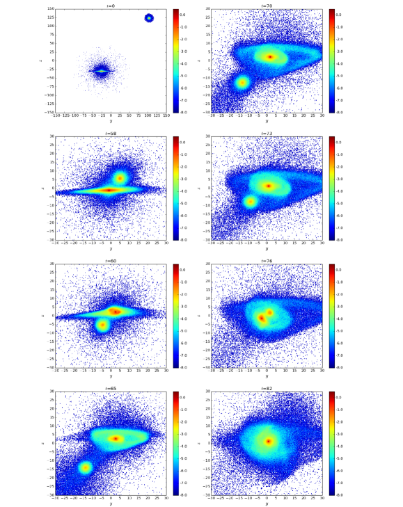
Figure 4: The evolution of the projected density of the stellar components, including the stellar disk, the bulge and the dwarf’s stellar part, on the $y-z$ plane in Si40. The unit of length is kpc. The unit of surface density is $10^{10}M_{\odot}$ kpc^-2, and the scale is logarithmic.

On the other hand, Fig. 3 and Fig. 4 give an example of the time evolution of the projected density of all stellar particles, including the stellar disk, the bulge, and the dwarf’s stellar component, on the $x-y$ and $y-z$ plane in the simulation Si40. At the beginning, i.e. $t=0$, the center of mass of the dwarf galaxy and the disk galaxy are separated with a distance 128.5 kpc on the y-axis and 153.2 kpc on the z-axis. Then, they approach and pass through each other from $t=58T_{s}$ to $t=59T_{s}$. Being a collision with inclination angle $i=40$ degrees, an elliptical ring is formed at $t=60T_{s}$. The ring is not azimuthally uniform, and the center of the disk galaxy shifts towards the $+y$ direction. Later on, the ring expands and the density of the ring decreases, as shown at $t=65T_{s}$. Due to the projection effect, it seems that, on the $x-y$ plane, the dwarf galaxy is connected with the ring. Besides, the location of the disk center, which has the highest projected density, does not move a lot, but the ring expands more towards the $+y$ direction. During this stage, the dwarf galaxy keeps moving away from the disk galaxy. From $t=70T_{s}$ to $t=75T_{s}$, the dwarf galaxy returns and has the second encounter.

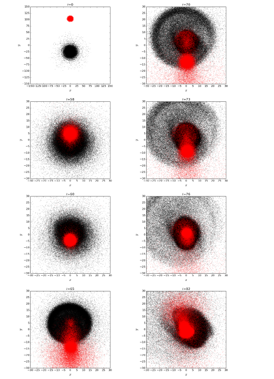
Figure 5: Time evolution of the stellar particles on the $x-y$ plane in Si40. The black dots represent the stellar disk and the bulge particles of the disk galaxy. The red dots represent the dwarf’s stellar particles. The unit of length is kpc.

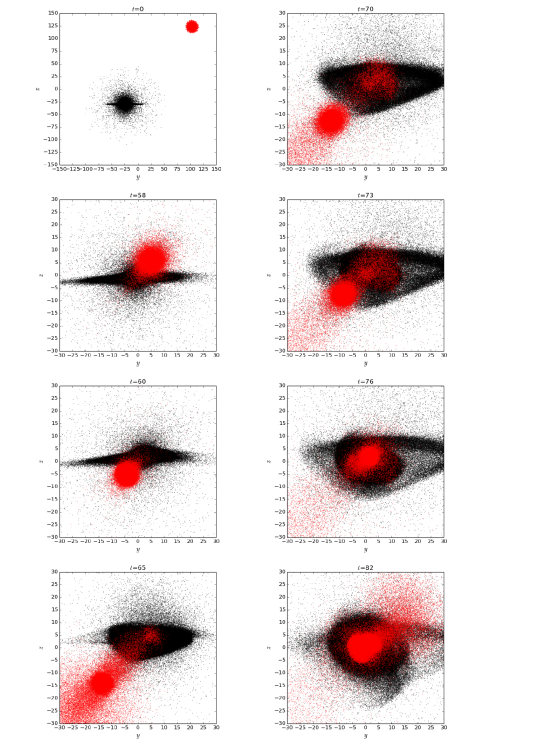
Figure 6: Time evolution of the stellar particles on the $y-z$ plane in Si40. The black dots represent the stellar disk and the bulge particles of the disk galaxy. The red dots represent the dwarf’s stellar particles. The unit of length is kpc.

Moreover, Fig. 5 and Fig. 6 are those snapshots in Fig. 3 and Fig. 4 but are plotted in terms of particle positions. The black dots represent the particles of the stellar disk and the bulge of the disk galaxy, while the red dots represent the dwarf’s stellar particles. The evolution of particle distributions of both galaxies can therefore be seen clearly. After the first collision, some dwarf’s stellar particles get trapped near the center of the disk galaxy, some have gone very far from the cores of both galaxies, and a certain fraction of particles follow the orbit of the dwarf galaxy. Comparing Fig. 5 with Fig. 3, it is obvious that the ring is mainly made of particles originally belonging to the disk galaxy. In the end, at $t=82T_{s}$, the disk galaxy and the dwarf galaxy merge.

In general, when a satellite galaxy falls into a major galaxy, the satellite experiences the dynamical friction from the stars and halo of the major galaxy. The satellite would lose some energy and have an orbital decay. A similar process was shown in Jiang and Binney (2000).

3.2 The Ring

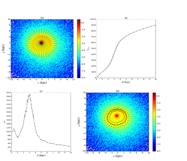
Figure 7: An example for the ellipse fitting process. (a) The projected density of the stellar components of the disk galaxy, including the stellar disk and the bulge, on the $x-y$ plane at $t=60T_{s}$ in simulation Si30. The azimuthal cells are also shown by those black grid-lines. (b) The number of accumulated particles, $N_{acc}$, contained in one azimuthal cell as a function of radius $R$. (c) The slope, $m$, of the curve $N_{acc}(R)$, as a function of radius $R$. The red triangle represents the maximum of the slope, and the blue triangle labels the minimum of the slope between the disk center and the ring region. The green dots represent the slope which is equal to the average of the maximum slope and the minimum slope, i.e. $m_{ave}$. (d) The fitting ellipse (black curve) overlaid on the projected density. The green dots represent the locations, $ri$ and $ro$, where the slopes of $N_{acc}(R)$ are equal to $m_{ave}$ for all different azimuthal cells. The black dots represent the locations which are given by $(ri+ro)/2$ for all different azimuthal cells.

From the snapshots in Figs. 3-4., it is likely that the collisions with non-zero inclination angle $i$ could produce elliptical rings. In order to understand the shape of elliptical rings, we develop a new method to determine the related parameters, such as semi-major axis, semi-minor axis, and eccentricity. The procedure is described below with an example demonstrated in Fig. 7.

First, the stellar components of the disk galaxy, including the bulge and the stellar disk, are projected on the $x-y$ plane. Then, we divide the space into small square cells, and calculate the projected density of the particles within each cell. The size of each cell is 0.2 kpc $\times$ 0.2 kpc. After that, taking the center of the cell which has the highest projected density as the coordinate center, we divide the space equally into 36 cells in the azimuthal direction as shown in Fig. 7 (a). Fig. 7 (a) shows the projected density on the $x-y$ plane at $t=60T_{s}$ in simulation Si30. The black lines represent the grid-lines, and the angle between two grid-lines is ten degrees. Following this, we calculate the accumulated number of particles $N_{acc}$ contained in each azimuthal cell as a function of radius $R$ (with 200 particles in each radial bin), as shown in Fig. 7 (b). From Fig. 7 (b), it shows that $N_{acc}$ increases rapidly within 0.5 kpc and then slows down from 0.5 to 1.5 kpc. After $R=$ 1.5 kpc, $N_{acc}$ increases rapidly again until R$\sim$4 kpc. Obviously, the concentration in the galactic center produces the rapid increment of $N_{acc}$ within 0.5 kpc, and the existence of a ring explains another rapid increment between 1.5 and 4 kpc.

To identify the ring region precisely, the slope of the curve in Fig. 7 (b) is plotted as a function of $R$ as shown in Fig. 7 (c). Thus, the black dots are the slope $m$ at different radius $R$. The red triangle labels the maximum of the slope, $m_{max}$, which should be located within the central part of the ring region. Between the disk center and the ring region, the blue triangle labels the minimum of the slope, $m_{min}$. Thus, the average of the maximum slope and the minimum slope could be calculated as $m_{ave}=(m_{max}+m_{min})/2$ and the corresponding inner radius $ri$ and outer radius $ro$, where the slopes are equal to $m_{ave}$, could be determined, as represented by the green dots in panel (c). The above is done for all 36 azimuthal cells. Therefore, for each azimuthal cell, we define the inner boundary of ring region to be $ri$, the outer boundary of ring region to be $ro$, the radial coordinate of the ring to be $(ri+ro)/2$. Thirty-six black dots in Fig. 7 (d) indicate the radial coordinates of the ring at different azimuthal cells, and the green dots represent the locations of $ri$ and $ro$.

Finally, those black dots are used to determine an ellipse following Gander et al. (1994), in which Gauss-Newton method (Gill, Murray & Wright 1981) is used. The best-fitting ellipse is obtained when the sum of the squares of the distances from the black dots to the ellipse is minimized. Thus, the black ellipse in Fig. 7 (d) shows our best fitting ellipse. The semi-major axis $R_{a}$, the semi-minor axis $R_{b}$, the eccentricity $e$, and the center of this ellipse can be determined correspondingly.

Moreover, because the elliptical ring is a pattern generated during the galactic collision, its center could be offset from the disk center. In order to determine this offset, we draw a straight line starting from the ellipse center, passing the disk center, and arriving at the ellipse boundary. The total length of this line $l$ and also the distance $d_{ed}$ from the ellipse center to the disk center can be calculated. The offset $p$, which is a dimensionless parameter, is defined as

$$p=\frac{d_{ed}}{l}.$$ (6)

Thus, when the disk center is close to the ellipse center, the offset $p$ is close to 0; when the disk center is close to the boundary of the ellipse, the offset $p$ is close to 1.

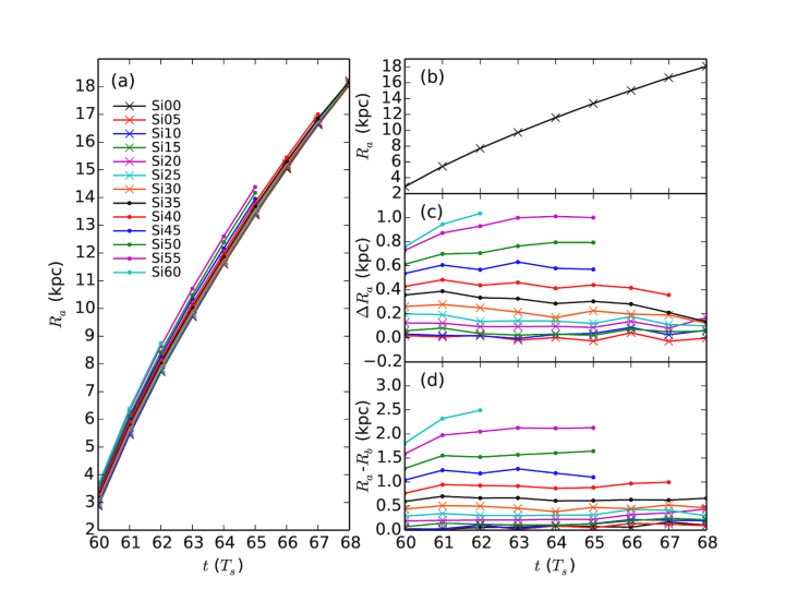
Figure 8: The evolution of the sizes of rings in simulations. Different lines represent different simulations, as indicated in panel (a). (a) The semi-major axis of the ring, $R_{a}$, as a function of time for different simulations. (b) The semi-major axis of the ring as a function of time for simulation Si00. (c) The differences of the semi-major axis between other simulations and Si00 as functions of time. (d) The differences between the semi-major axis and the semi-minor axis as functions of time for different simulations.

Here we present the results determined through the above method. Fig. 8 (a) shows the time evolution of the semi-major axis of rings in all 13 simulations. The lines with different colors and different symbols correspond to the simulations with different inclination angles, as indicated in panel (a). The rings all form at $t=60T_{s}$ but exist in a shorter duration when the collisions have larger inclination angles. For example, the lifetime of the ring in Si60 is only 2$T_{s}$, that is from $t$=60 to $t$=62$T_{s}$. To understand the effect of the inclination angle on the semi-major axis of the ring, the ring in Si00 is used as a standard. Fig. 8 (b) shows the semi-major axis of the ring as a function of time in Si00 only. Then, Fig. 8 (c) shows the differences of the semi-major axis of the ring, $\Delta R_{a}$, between other simulations and Si00 at different times. For example, the semi-major axis of the ring at $t$=62$T_{s}$ in Si00 and Si40 are 7.71 and 8.15, respectively. Therefore, $\Delta R_{a}$ between the simulation Si00 and Si40 at $t$=62$T_{s}$ is 0.44, as shown in panel (c) (red line with dotted symbols). Thus, from panel (c), we can see that there is no significant difference between Si00 and the simulations with inclination angles smaller than 15 degrees. It means that the rings produced by the collisions with inclination angles smaller than 15 degrees are similar as the rings produced by the head-on collision.

Finally, Fig. 8 (d) presents the differences between the semi-major axis, $R_{a}$, and the semi-minor axis, $R_{b}$, of these rings as functions of time. The difference between these two axes, i.e. $R_{a}-R_{b}$, is larger when the collision has larger inclination angle. Please note for the head-on collision, i.e. Si00, $R_{a}-R_{b}$ is very small but not completely zero. This leads to an eccentricity about 0.1. Thus, in this paper, any ring with eccentricity about 0.1 is considered to be equivalent to a circular ring. In fact, as we can see in panel (c), all simulations with inclination angle smaller than 15 degrees present very similar results and to distinguish them is beyond the scope of this paper.

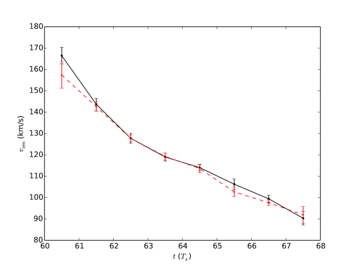
Figure 9: The evolution of the out-moving speeds, $v_{om}$, of rings in simulations. The black line represents the average of the out-moving speeds of the semi-major axis for 13 simulations. The red line is for the semi-minor axis. The error bar indicates one standard deviation.

On the other hand, because $R_{a}$ increases with time, the out-moving speed $v_{om}$ of the semi-major axis, $R_{a}$, is defined as $(R_{a}(T_{2})-R_{a}(T_{1}))/T_{s}$, where $R_{a}(T_{2})-R_{a}(T_{1})$ is the variation of the semi-major axis within one $T_{s}$ from $T_{1}$ to $T_{2}$. We also define the out-moving speed of the semi-minor axis similarly. The average of the out-moving speed for all simulations is shown in Fig. 9. The black line presents the out-moving speed of the semi-major-axis, and the red line is for the semi-minor axis. The error bar indicates one standard deviation. The largest standard deviation in the figure is 6.1 km/s. Thus, the inclination angle has no significant effect on the out-moving speeds of ring patterns. In addition, it is apparent that the out-moving speeds of the semi-major axis and the semi-minor axis are similar and both decrease gradually as functions of time.

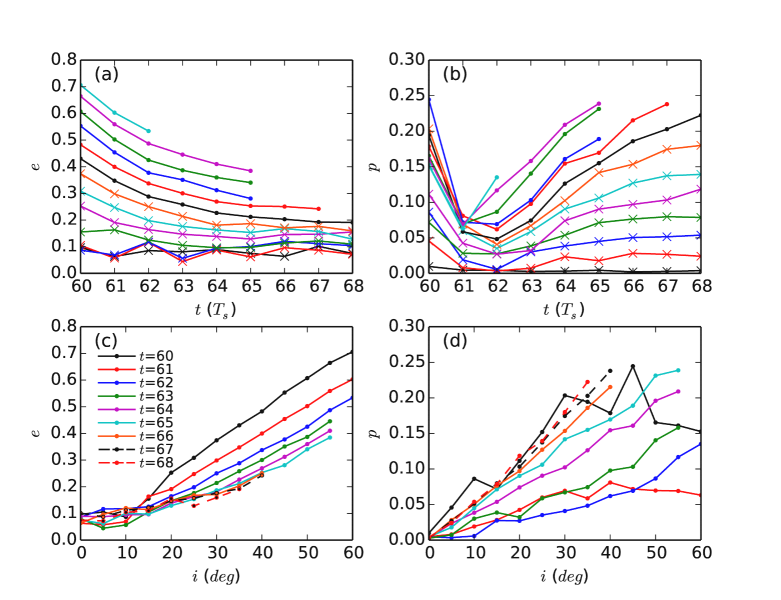
Figure 10: The properties of rings in simulations. For panel (a) and (b), different lines are for different simulations as indicated in Fig. 8. (a) The eccentricity as a function of time. (b) The offset $p$ as a function of time. For panel (c) and (d), different lines represent different simulation time, as indicated in panel (c). (c) The eccentricity as a function of the inclination angle, $i$. (d) The offset $p$ as a function of the inclination angle, $i$.

The results of the eccentricity and offset of rings are presented here. The eccentricity can be calculated easily from the semi-major axis $R_{a}$ and semi-minor axis $R_{b}$. Fig. 10 (a) presents the time evolution of the ring eccentricity $e$ in all 13 simulations. Different lines represent different simulations as indicated in Fig. 8 (a). When the inclination angle is smaller than 15 degrees, the ring eccentricity is about 0.1. On the other hand, for the simulations with inclination angles larger than 15 degrees, the eccentricity of the ring decreases slowly with time.

Fig. 10 (b) presents the offset $p$ as a function of time. Different lines are for different simulations as in panel (a). It shows that the disk center is very close to the center of the ellipse when the inclination angle of the collision is 0, i.e. the simulation Si00. Besides, for all simulations, the offset $p$ is larger at the beginning and then becomes smaller at $t=61T_{s}$. This is because at the beginning of the collision, the disk center moves towards $+y$ direction and gets closer to the boundary of the ellipse, as the example shown in Fig. 3 $t=60T_{s}$. After that, the ring expands, and the ellipse center shifts toward $+y$ direction as well. However, the location of the disk center does not move significantly after $t=60T_{s}$. Thus, at $t=61T_{s}$, the disk center and the ellipse center are close to each other and the offset $p$ becomes smaller. After $t=61T_{s}$, the ellipse center shifts toward $+y$ direction continuously, so the offset $p$ increases slightly.

Fig. 10 (c) and (d) present the ring eccentricity $e$ and the offset $p$ as functions of the inclination angle of the collisions, respectively. For these two panels, different lines represent different times, as indicated in panel (c). From panel (c), we can see that for the collisions with inclination angle larger than 15 degrees, the eccentricity increases steadily. For example, at $t=60T_{s}$, the eccentricity in Si20, Si40 and Si60 are 0.25, 0.48 and 0.71, respectively. From panel (d), after $t=62T_{s}$, it can be seen that at the same simulation time, the ring has larger offset $p$ when the collision has larger inclination angle.

In fact, the most striking feature shown in Fig. 10 (c) is that for $i=15,20,...,55$ degrees, and $t=60,61,...,64T_{s}$, the results are simply straight lines with slightly different slopes. The information of slope differences is actually in Fig. 10 (a), which shows that the eccentricity varies with time as $-\sqrt{t}$ approximately. Thus, using the data points for the above $i$ and $t$, an analytic formula expressing the eccentricity as a function of $t$ and $i$ on $t-i$ plane can be obtained:

$$e(t,i)=\{\beta_{1}-\beta_{2}\sqrt{t/T_{s}-t_{f}/T_{s}}\}{i}/{\rm degree},$$ (7)

where $\beta_{1}=0.0120$, $\beta_{2}=0.0025$, $t_{f}=60T_{s}$. Though this equation is unlikely to fit all simulational results perfectly. It is a good approximation which could be a useful tool for the interpretations of elliptical ring systems.

4 Conclusions

Motivated by the existence of elliptical rings in disk galaxies, the effect of the inclination angle between the merging pair on the morphology of elliptical rings is investigated. This is the first time to have such high resolution on the inclination and thus the association between the inclination and the shape of ring galaxies are quantified.

The results have shown that the elliptical rings could be produced by the collisions with inclination angles from 15 to 60 degrees. The elliptical ring’s eccentricity ranges from 0.1 to 0.7 and the offset $p$ is from nearly 0 to about 0.25. The out-moving speeds of ring patterns are not affected by the inclination but decays with time, from about 170 km/s to 90 km/s.

We confirm that the galaxy pairs with larger inclination angles can produce elliptical rings with larger eccentricities. The linear dependence between eccentricity and inclination leads to an analytic formula in which the eccentricity is expressed as a function of time and inclination. This simple rule deriving from the results of N-body simulations shall be very helpful for the future investigation of merging histories of galactic systems with elliptical rings.

Figure 1: The virial ratio $2K/|U|$ (top panel) and Lagrangian radii (bottom panel) of the disk galaxy as a function of time $t$, where the unit of $t$ is its dynamical time.

Figure 2: The evolution of simulations Si00, Si20 and Si40. Panels (a)-(f) show the locations of the disk galaxy and the dwarf galaxy on $y$ and $z$ axis as functions of time in Si00, Si20 and Si40, respectively. The solid and long dashed curves correspond to the centers of mass of the whole disk galaxy and the whole dwarf galaxy. The short dashed and dotted curves represent the centers of mass of the disk’s stellar components (including both the bulge and the stellar disk) and the dwarf’s stellar component.

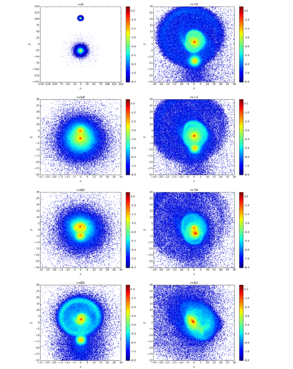
Figure 3: The evolution of the projected density of the stellar components, including the stellar disk, the bulge and the dwarf’s stellar part, on the $x-y$ plane in Si40. The unit of length is kpc. The unit of surface density is $10^{10}M_{\odot}$ kpc^-2, and the scale is logarithmic.

References

- Binney et al. (1998) Binney, J., Jiang, I.-G., & Dutta, S. 1998, MNRAS, 297, 1237
- Binney & Tremaine (1987) Binney, J., Tremaine, S. 1987, Galactic Dynamics (Princeton Univ. Press)
- Elmegreen & Elmegreen (2006) Elmegreen, D. M., Elmegreen, B. G. 2006, ApJ, 651, 676
- (4) Fiacconi, D., Mapelli, M., Ripamonti, E., Colpi, M. 2012, MNRAS, 425, 2255
- (5) Gander, W., Golub, G. H., Strebel, R. 1994, BIT Numerical Mathematics, 34, 558
- (6) Gerber, R. A., Lamb, S. A., Balsara, D. S. 1992, ApJ, 399, L51
- (7) Gill, E., Murray, W., Wright, M. H. 1981, Practical Optimization (Academic Press, New York)
- Hernquist (1990) Hernquist, L. 1990, ApJ, 356, 359
- Hernquist (1993) Hernquist, L. 1993, ApJS, 86, 389
- Hoag (1950) Hoag, A. A. 1950, AJ, 55, 170
- Jiang (2000) Jiang, I.-G., Binney, J. 2000, MNRAS, 314, 468
- Lynds & Toomre (1976) Lynds, R., Toomre, A. 1976, ApJ, 209, 382
- Madore, Nelson & Petrillo (2009) Madore, B. F., Nelson, E., Petrillo, K. 2009, ApJS, 181, 572
- Mapelli (2012) Mapelli, M., Mayer, L. 2012, MNRAS, 420, 1158
- Read et. al. (2006) Read, J. I., Wilkinson, M. I., Evans, N. W., Gilmore, G., Kleyna, J. T. 2006, MNRAS, 367, 387
- Smith et al. (2012) Smith, R., Lane, R. R., Conn, B. C., Fellhauer, M. 2012, MNRAS, 423, 543
- Springel, Yoshida, & White (2001) Springel, V., Yoshida, N., White, S. D. M. 2001, NewA, 6, 79
- (18) Struck-Marcell, C. 1990, AJ, 99, 71
- (19) Struck-Marcell, C., Lotan, P. 1990, ApJ, 358, 99
- Wa (1990) Wakamatsu, K. 1990, ApJ, 348, 448
- Wong (2006) Wong, O. I., et al. 2006, MNRAS, 370, 1607
- Wu & Jiang (2009) Wu, Y.-T., Jiang, I.-G. 2009, MNRAS, 399, 628
- Wu & Jiang (2011) Wu, Y.-T., Jiang, I.-G. 2011, IAU Symposium, 271, 102
- Wu & Jiang (2012) Wu, Y.-T., Jiang, I.-G. 2012, ApJ, 745, 105