Abstract

In this paper, we investigate the modification of our expressions developed for the model–independent data analysis procedure of the reconstruction of the (time–averaged) one–dimensional velocity distribution of Galactic Weakly Interacting Massive Particles (WIMPs) with a non–negligible experimental threshold energy. Our numerical simulations show that, for a minimal reconstructable velocity of as high as ${\cal O}(200)$ km/s, our model–independent modification of the estimator for the normalization constant could provide precise reconstructed velocity distribution points to match the true WIMP velocity distribution with a  $\stackrel{{\scriptstyle\textstyle<}}{{\sim}}$  10% bias.

1 Introduction

Currently, direct Dark Matter detection experiments searching for Weakly Interacting Massive Particles (WIMPs) are one of the promising methods for understanding the nature of Dark Matter (DM) and identifying them among new particles produced at colliders as well as studying the (sub)structure of our Galactic halo [1, 2, 3, 4].

In our earlier work [5], we developed model–independent methods for reconstructing the (moments of the) time–averaged one–dimensional velocity distribution of halo WIMPs by using the measured recoil energies directly. However, with a few hundreds or even thousands recorded WIMP events, only estimates of the reconstructed velocity distribution with pretty large statistical uncertainties at a few ($<$ 10) points could be obtained. Hence, in order to provide more detailed information about the WIMP velocity distribution, we introduced the Bayesian analysis into our reconstruction procedure for concretely determining, e.g. the position of the peak of the one–dimensional velocity distribution function and the values of the characteristic Solar and Earth’s Galactic velocities [6].

In our Monte Carlo simulations presented in Refs. [5, 6], the minimal experimental cut–off energies of data sets to be analyzed are assumed to be negligible. For experiments with heavy target nuclei, e.g. Ge or Xe, and once WIMPs are heavy ($\>\raisebox{-3.01385pt}{$\stackrel{{\scriptstyle\textstyle>}}{{\sim}}$}\>~{}100$ GeV), the systematic bias caused by this assumption should be acceptable. However, once WIMPs are light ($\>\raisebox{-3.01385pt}{$\stackrel{{\scriptstyle\textstyle<}}{{\sim}}$}\>~{}50$ GeV) and a light target nucleus, e.g. Si or Ar, is used for reconstructing the WIMP velocity distribution $f_{1}(v)$, effects of a non–negligible threshold energy has to be considered and the estimate of the normalization constant of $f_{1}(v)$ would need to be modified properly. Therefore, as a supplement of our earlier works, we consider in this paper the needed modification of the normalization constant of $f_{1}(v)$ for the general case with a non–negligible experimental threshold energy.

The remainder of this paper is organized as follows. In Sec. 2, we first review the model–independent method for reconstructing the time–averaged one–dimensional velocity distribution of halo WIMPs by using data from direct DM detection experiments directly. Then, in Sec. 3, we develop the modification of the normalization constant of $f_{1}(v)$ for a non–zero minimal experimental cut–off energy step by step. Numerical results of the modified reconstruction of the WIMP velocity distribution based on the Monte Carlo simulation will be given. A systematic bias in this model–independent modification will be discussed particularly. We conclude in Sec. 4. Some technical details for our analysis will be given in Appendix.

2 Model–independent reconstruction of the one–dimensional WIMP velocity distribution

In this section, we first review in brief the model–independent method for reconstructing the (time–averaged) one–dimensional WIMP velocity distribution by using experimental data, i.e. measured recoil energies, directly from direct detection experiments. Detailed derivations and discussions can be found in Ref. [5].

2.1 From the recoil spectrum

The basic expression for the differential event rate for elastic WIMP–nucleus scattering is given by [1]:

$$\frac{dR}{dQ}={\cal A}F^{2}(Q)\int_{v_{\rm min}}^{v_{\rm max}}\left[\frac{f_{1}(v)}{v}\right]dv~{}\!.$$ (1)

Here $R$ is the direct detection event rate, i.e. the number of events per unit time and unit mass of detector material, $Q$ is the energy deposited in the detector, $F(Q)$ is the elastic nuclear form factor, $f_{1}(v)$ is the one–dimensional velocity distribution function of the WIMPs impinging on the detector, $v$ is the absolute value of the WIMP velocity in the laboratory frame. The constant coefficient ${\cal A}$ is defined as ${\cal A}\equiv\rho_{0}\sigma_{0}/2m_{\chi}m_{\rm r,N}^{2}$, where $\rho_{0}$ is the WIMP density near the Earth and $\sigma_{0}$ is the total cross section ignoring the form factor suppression. The reduced mass $m_{\rm r,N}$ is defined by $m_{\rm r,N}\equiv m_{\chi}m_{\rm N}/\left(m_{\chi}+m_{\rm N}\right)$, where $m_{\chi}$ is the WIMP mass and $m_{\rm N}$ that of the target nucleus. Finally, $v_{\rm min}$ is the minimal incoming velocity of incident WIMPs that can deposit the energy $Q$ in the detector: $v_{\rm min}=\alpha\sqrt{Q}$ with the transformation constant

$$\alpha\equiv\sqrt{\frac{m_{\rm N}}{2m_{\rm r,N}^{2}}}~{}\!,$$ (2)

and $v_{\rm max}$ is the maximal WIMP velocity in the Earth’s reference frame, which is related to the escape velocity from our Galaxy at the position of the Solar system, $v_{\rm esc}$.

In our earlier work [5], it was found that, by using a time–averaged recoil spectrum $dR/dQ$ and assuming that no directional information exists, the normalized one–dimensional velocity distribution function of incident WIMPs can be solved from Eq. (1) directly as

$$f_{1}(v)={\cal N}\left\{-2Q\cdot\frac{d}{dQ}\left[\frac{1}{F^{2}(Q)}\left(\frac{dR}{dQ}\right)\right]\right\}_{Q=v^{2}/\alpha^{2}}~{}\!,$$ (3)

where the normalization condition:

$$\int_{0}^{\infty}f_{1}(v)~{}\!dv=1$$ (4)

has been used and thus the normalization constant ${\cal N}$ is given by

$${\cal N}=\frac{2}{\alpha}\left\{\int_{0}^{\infty}\frac{1}{\sqrt{Q}}\left[\frac{1}{F^{2}(Q)}\left(\frac{dR}{dQ}\right)\right]dQ\right\}^{-1}~{}\!.$$ (5)

Here the integral goes over the entire physically allowed range of recoil energies: starting at $Q=0$, and the upper limit of the integral has been written as $\infty$. Note that, the velocity distribution function of halo WIMPs reconstructed by Eq. (3) is independent of the local WIMP density $\rho_{0}$ as well as of the WIMP–nucleus cross section $\sigma_{0}$. However, not only the overall normalization constant ${\cal N}$ given in Eq. (5), but also the shape of the velocity distribution transformed through $Q=v^{2}/\alpha^{2}$ depends on the WIMP mass $m_{\chi}$ (involved in the coefficient $\alpha$ defined in Eq. (2)).

2.2 From experimental data directly

In order to avoid some model dependence during giving a functional form for the recoil spectrum $dR/dQ$ needed in Eqs. (3) and (5), expressions that allow to reconstruct $f_{1}(v)$ directly from data (i.e. measured recoil energies) have also been developed [5].

Consider experimental data described by

$${\textstyle Q_{n}-\frac{b_{n}}{2}}\leq Q_{n,i}\leq{\textstyle Q_{n}+\frac{b_{n}}{2}}~{}\!,~{}~{}~{}~{}~{}~{}~{}~{}~{}~{}~{}~{}i=1,~{}2,~{}\cdots,~{}N_{n},~{}n=1,~{}2,~{}\cdots,~{}B.$$ (6)

Here the entire experimental possible energy range between the minimal and maximal cut–offs $Q_{\rm min}$ and $Q_{\rm max}$ has been divided into $B$ bins with central points $Q_{n}$ and widths $b_{n}$. In each bin, $N_{n}$ events will be recorded. Since the recoil spectrum $dR/dQ$ is expected to be approximately exponential, in order to approximate the spectrum in a rather wider range, instead of the conventional standard linear approximation, the following exponential ansatz for the measured recoil spectrum (before normalized by the exposure ${\cal E}$) in the $n$th bin has been introduced [5]:

$$\left(\frac{dR}{dQ}\right)_{{\rm expt},~{}\!n}\equiv\left(\frac{dR}{dQ}\right)_{{\rm expt},~{}\!Q\simeq Q_{n}}\equiv r_{n}~{}\!e^{k_{n}(Q-Q_{s,n})}~{}\!.$$ (7)

Here $r_{n}=N_{n}/b_{n}$ is the standard estimator for $(dR/dQ)_{\rm expt}$ at $Q=Q_{n}$, $k_{n}$ is the logarithmic slope of the recoil spectrum in the $n$th $Q-$bin, which can be computed numerically from the average value of the measured recoil energies in this bin:

$$\overline{Q-Q_{n}}|_{n}=\left(\frac{b_{n}}{2}\right)\coth\left(\frac{k_{n}b_{n}}{2}\right)-\frac{1}{k_{n}}~{}\!,$$ (8)

where

$$\overline{(Q-Q_{n})^{\lambda}}|_{n}\equiv\frac{1}{N_{n}}\sum_{i=1}^{N_{n}}\left(Q_{n,i}-Q_{n}\right)^{\lambda}~{}\!.$$ (9)

Then the shifted point $Q_{s,n}$ in the ansatz (7), at which the leading systematic error due to the ansatz is minimal [5], can be estimated by

$$Q_{s,n}=Q_{n}+\frac{1}{k_{n}}\ln\left[\frac{\sinh(k_{n}b_{n}/2)}{k_{n}b_{n}/2}\right]~{}\!.$$ (10)

Note that $Q_{s,n}$ differs from the central point of the $n$th bin, $Q_{n}$. Finally, substituting the ansatz (7) into Eq. (3) and then letting $Q=Q_{s,n}$, we can obtain that

$$f_{1,{\rm rec}}(v_{s,n})={\cal N}\Bigg{[}\frac{2Q_{s,n}r_{n}}{F^{2}(Q_{s,n})}\Bigg{]}\left[\frac{d}{dQ}\ln F^{2}(Q)\bigg{|}_{Q=Q_{s,n}}-k_{n}\right]~{}\!.$$ (11)

Here $v_{s,n}=\alpha\sqrt{Q_{s,n}}$, and the normalization constant ${\cal N}$ given in Eq. (5) can be estimated directly from the data by

$${\cal N}=\frac{2}{\alpha}\left[\sum_{a}\frac{1}{\sqrt{Q_{a}}~{}\!F^{2}(Q_{a})}\right]^{-1}~{}\!,$$ (12)

where the sum runs over all events in the sample.

2.3 Windowing the data set

In order to reduce the statistical uncertainty on the velocity distribution reconstructed by Eq. (11) and some uncontrolled systematic errors caused by neglecting terms of higher powers of $Q-Q_{n}$, as well as to offer a reasonable number of reconstructable velocity points $v_{s,n}$ of $f_{1}(v)$, it has been introduced in Ref. [5] that one can first collect experimental data in relatively small bins with linearly increased widths and then combining varying numbers of bins into overlapping “windows”. Thus, we set that the bin widths satisfy $b_{n}=b_{1}+(n-1)\delta$, Hence,

$$Q_{n}=Q_{\rm min}+\left(n-\frac{1}{2}\right)b_{1}+\left[\frac{(n-1)^{2}}{2}\right]\delta~{}\!.$$ (13)

Here the increment $\delta$ satisfies $\delta=2\Big{(}Q_{\rm max}-Q_{\rm min}-Bb_{1}\Big{)}/B(B-1)$, $B$ being the total number of bins, and $Q_{\rm(min,max)}$ are the experimental minimal and maximal cut–off energies. Assume up to $n_{W}$ bins are collected into a window, with smaller windows at the borders of the range of $Q$.

In order to distinguish the numbers of bins and windows, hereafter Latin indices $n,~{}m,~{}\cdots$ are used to label bins, and Greek indices $\mu,~{}\nu,~{}\cdots$ to label windows. For $1\leq\mu\leq n_{W}$, the $\mu$th window simply consists of the first $\mu$ bins; for $n_{W}\leq\mu\leq B$, the $\mu$th window consists of bins $\mu-n_{W}+1,~{}\mu-n_{W}+2,~{}\cdots,~{}\mu$; and for $B\leq\mu\leq B+n_{W}-1$, the $\mu$th window consists of the last $n_{W}-(\mu-B)$ bins. This can also be described by introducing the indices $n_{\mu-}$ and $n_{\mu+}$ which label the first and last bins contributing to the $\mu$th window, with

$$n_{\mu-}=\left\{\begin{array}[]{l c l}1,&{}{}{}{}{}{}\hfil&{\rm for}~{}\mu\leq n_{W},\\ \mu-n_{W}+1,&&{\rm for}~{}\mu\geq n_{W},\end{array}\right.$$ (14a)

and

$$n_{\mu+}=\left\{\begin{array}[]{l c l}\mu,&{}{}{}{}{}{}\hfil&{\rm for}~{}\mu\leq B,\\ B,&&{\rm for}~{}\mu\geq B.\end{array}\right.$$ (14b)

The total number of windows defined through Eqs. (14a) and (14b) is evidently $W=B+n_{W}-1$, i.e. $1\leq\mu\leq B+n_{W}-1$.

For a “windowed” data set, one can easily calculate the number of events per window as

$$N_{\mu}=\sum_{n=n_{\mu-}}^{n_{\mu+}}N_{n}~{}\!,$$ (15)

as well as, the average value of the measured recoil energies

$$\overline{Q-Q_{\mu}}|_{\mu}=\frac{1}{N_{\mu}}\left(\sum_{n=n_{\mu-}}^{n_{\mu+}}N_{n}\overline{Q}|_{n}\right)-Q_{\mu}~{}\!,$$ (16)

where $Q_{\mu}$ is the central point of the $\mu$th window. The exponential ansatz in Eq. (7) is now assumed to hold over an entire window. We can then estimate the prefactor as $r_{\mu}=N_{\mu}/w_{\mu}$, $w_{\mu}$ being the width of the $\mu$th window. The logarithmic slope of the recoil spectrum in the $\mu$th window, $k_{\mu}$, as well as the shifted point $Q_{s,\mu}$ (from the central point of each “window”, $Q_{\mu}$) can be calculated as in Eqs. (8) and (10) with “bin” quantities replaced by “window” quantities. Finally, the covariance matrix of the estimates of $f_{1}(v)$ at adjacent values of $v_{s,\mu}=\alpha\sqrt{Q_{s,\mu}}$ is given by

$${\rm cov}\Big{(}f_{1,{\rm rec}}(v_{s,\mu}),f_{1,{\rm rec}}(v_{s,\nu})\Big{)}$$ (17)

$$= \left[\frac{f_{1,{\rm rec}}(v_{s,\mu})f_{1,{\rm rec}}(v_{s,\nu})}{r_{\mu}r_{\nu}}\right]{\rm cov}\left(r_{\mu},r_{\nu}\right)+\left(2{\cal N}\right)^{2}\left[\frac{Q_{s,\mu}Q_{s,\nu}r_{\mu}r_{\nu}}{F^{2}(Q_{s,\mu})F^{2}(Q_{s,\nu})}\right]{\rm cov}\left(k_{\mu},k_{\nu}\right)$$

$$~{}~{}~{}~{}~{}~{}~{}~{}~{}~{}~{}~{}-{\cal N}\left\{\left[\frac{f_{1,{\rm rec}}(v_{s,\mu})}{r_{\mu}}\right]\left[\frac{2Q_{s,\nu}r_{\nu}}{F^{2}(Q_{s,\nu})}\right]{\rm cov}\left(r_{\mu},k_{\nu}\right)+\Big{(}\mu\longleftrightarrow\nu\Big{)}\right\}~{}\!.$$

2.4 Numerical results

In this section, we present reconstruction results of the one–dimensional WIMP velocity distribution before taking the modification of the normalization constant of $f_{1}(v)$.

First of all, since the lighter the WIMP mass, the more problematic the non–negligible experimental threshold energy, a light input WIMP mass of $m_{\chi}=25$ GeV has been considered in our simulations. As discussed and shown in Ref. [7], with ${\cal O}(500)$ recorded events (in one data set), the (light) input WIMP masses can be reconstructed pretty precisely with only $\sim$ 10% (a few GeV) statistical uncertainties (more simulation results can also be found in Ref. [6]). Thus, in our simulations demonstrated here and in the next section, the reconstructed WIMP mass $m_{\chi}$ involved in the coefficient $\alpha$ for estimating the reconstructed points $v_{s,\mu}$ as well as the normalization constant ${\cal N}$ has been assumed to be known precisely with a negligible uncertainty.

As in Ref. [5], ${}^{76}{\rm Ge}$ has been chosen as our detector material for reconstructing $f_{1}(v)$. As in Refs. [5, 6], the WIMP–nucleus cross section appearing in the expression (1) for the recoil spectrum $dR/dQ$ has been assumed to be only spin–independent (SI), $\sigma_{\chi{\rm p}}^{\rm SI}=10^{-9}$ pb, and the commonly used analytic form for the elastic nuclear form factor:

$$F_{\rm SI}^{2}(Q)=\left[\frac{3j_{1}(qR_{1})}{qR_{1}}\right]^{2}e^{-(qs)^{2}}$$ (18)

has been adopted. Here $Q$ is the recoil energy transferred from the incident WIMP to the target nucleus, $j_{1}(x)$ is a spherical Bessel function, $q=\sqrt{2m_{\rm N}Q}$ is the transferred 3-momentum, for the effective nuclear radius we use $R_{1}=\sqrt{R_{A}^{2}-5s^{2}}$ with $R_{A}\simeq 1.2~{}\!A^{1/3}~{}{\rm fm}$ and a nuclear skin thickness $s\simeq 1~{}{\rm fm}$.

By taking into account the orbital motion of the Solar system around our Galaxy as well as that of the Earth around the Sun, the shifted Maxwellian velocity distribution of halo WIMPs has been given by [1, 5]:

$$f_{1,{\rm sh}}(v)=\frac{1}{\sqrt{\pi}}\left(\frac{v}{v_{0}v_{\rm e}}\right)\Big{[}e^{-(v-v_{\rm e})^{2}/v_{0}^{2}}-e^{-(v+v_{\rm e})^{2}/v_{0}^{2}}\Big{]}~{}\!.$$ (19)

Here $v_{0}\simeq 220$ km/s is the Solar orbital speed around the Galactic center, and $v_{\rm e}$ is the time-–dependent Earth’s velocity in the Galactic frame [8, 1]:

$$v_{\rm e}(t)=v_{0}\left[1.05+0.07\cos\left(\frac{2\pi(t-t_{\rm p})}{1~{}{\rm yr}}\right)\right]~{}\!,$$ (20)

with $t_{\rm p}\simeq$ June 2nd, the date on which the velocity of the Earth relative to the WIMP halo is maximal. Additionally, a common maximal cut–off on the one–dimensional WIMP velocity distribution has been set as $v_{\rm max}=700$ km/s.

Figure 1: The reconstructed (rough) velocity distribution (black crosses) with a ${}^{76}{\rm Ge}$ target for an input WIMP mass of $m_{\chi}=25$ GeV and an experimental threshold energy of $Q_{\rm min}=2$ keV. The vertical error bars show the square roots of the diagonal entries of the covariance matrix estimated by Eq. (17), whereas the horizontal bars indicate the sizes of the windows used for estimating $f_{1,{\rm rec}}(v_{s,\mu})$ by Eq. (11). The solid red curve is the generating shifted Maxwellian velocity distribution with an input value of $v_{0}=220$ km/s. See the text for further details.

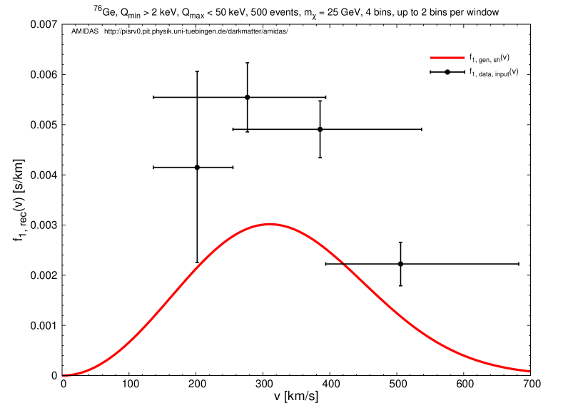
In our simulation shown in Fig. 1, the experimental threshold energy has been set as $Q_{\rm min}=2$ keV. Due to the maximal cut–off on the one–dimensional WIMP velocity distribution, $v_{\rm max}$, a kinematic maximal cut–off energy,

$$Q_{\rm max,kin}=\frac{v_{\rm max}^{2}}{\alpha^{2}}~{}\!,$$ (21)

has to be considered. Since for our target ${}^{76}{\rm Ge}$ it is only $Q_{\rm max,kin,Ge}=52.65$ keV, the maximal experimental cut–off energy has been set to be only $Q_{\rm max}=50$ keV. Meanwhile, since the lighter the WIMP mass, the steeper the expected recoil energy spectrum, $b_{1}=5$ keV width of the first energy bin has been used and the energy range between $Q_{\rm min}$ and $Q_{\rm max}$ has been divided into only four bins ($B=4$); up to two bins have been combined to a window and thus four windows ($W=4$) will be reconstructed [6]. Additionally, we assumed that all experimental systematic uncertainties as well as the uncertainty on the measurement of the recoil energy could be ignored. 5,000 experiments with 500 total events on average in one experiment have been simulated.

In Fig. 1, we show the reconstructed (rough) velocity distribution (black crosses) with a ${}^{76}{\rm Ge}$ target. The vertical error bars show the square roots of the diagonal entries of the covariance matrix estimated by Eq. (17), whereas the horizontal bars indicate the sizes of the windows used for estimating $f_{1,{\rm rec}}(v_{s,\mu})$ by Eq. (11). As a comparison, the solid red curve indicates the generating shifted Maxwellian velocity distribution with an input value of $v_{0}=220$ km/s. It can be seen clearly that the reconstructed velocity distribution is around two times overestimated. This indicates in turn that, by using Eq. (12), the normalization constant ${\cal N}$ of the velocity distribution function $f_{1}(v)$ is underestimated as only the half! Remind that the experimental threshold energy used here is as low as only 2 keV and the corresponding minimal cut–off of the velocity distribution is 134.44 km/s (see also Fig. 2).

3 Modification of the estimator for the normalization constant ${\cal N}$

In this section, we take into account the effect of a non–negligible experimental threshold energy ($Q_{\rm min}>0$) and introduce a model–independent modification of the estimator for the normalization constant ${\cal N}$ step by step.

3.1 Non–zero minimal cut–off velocity

First, we consider the minimal cut–off of the velocity distribution due to the non–zero experimental threshold energy, $v_{\rm min}(Q_{\rm min})\equiv v_{\rm min}^{\ast}$, in the use of the normalization condition (4). From Eq. (3), since $v=\alpha\sqrt{Q}$, by using integration by parts, we can obtain that

$$\int_{v_{\rm min}^{\ast}}^{v_{\rm max}}f_{1}(v)~{}\!dv = {\cal N}\int_{Q_{\rm min}}^{Q_{\rm max}^{\ast}}\left\{-2Q\cdot\frac{d}{dQ}\left[\frac{1}{F^{2}(Q)}\left(\frac{dR}{dQ}\right)\right]\right\}\left(\frac{\alpha}{2\sqrt{Q}}\right)dQ$$ (22)

$$= {\cal N}\left(\frac{\alpha}{2}\right)\left\{\frac{2Q_{\rm min}^{1/2}}{F^{2}(Q_{\rm min})}\left(\frac{dR}{dQ}\right)_{Q=Q_{\rm min}}+\int_{Q_{\rm min}}^{Q_{\rm max}^{\ast}}\frac{1}{\sqrt{Q}}\left[\frac{1}{F^{2}(Q)}\left(\frac{dR}{dQ}\right)\right]dQ\right\}$$

$$= {\cal N}\left(\frac{\alpha}{2}\right)\left[\frac{2Q_{\rm min}^{1/2}r(Q_{\rm min})}{F^{2}(Q_{\rm min})}+I_{0}(Q_{\rm min},Q_{\rm max}^{\ast})\right]~{}\!.$$

Here we define $Q_{\rm max}^{\ast}\equiv{\rm min}\left(Q_{\rm max},~{}Q_{\rm max,kin}\right)$, the smaller one between the experimental and kinematic cut–off energies and can be understood as the upper bound of the recoil energy of the recorded events; $Q_{\rm(min,max)}$ are the experimental minimal and maximal cut–off energies. Since the WIMP–nucleus scattering spectrum is expected to be exponential, the term of $\left(dR/dQ\right)_{Q=Q_{\rm max}^{\ast}}$ has been ignored here, whereas

$$r(Q_{\rm min})\equiv\left(\frac{dR}{dQ}\right)_{{\rm expt},~{}\!Q=Q_{\rm min}}=r_{1}~{}\!e^{k_{1}(Q_{\rm min}-Q_{s,1})}$$ (23)

with $r_{1}=N_{1}/b_{1}$, an estimated value of the measured recoil spectrum $(dR/dQ)_{\rm expt}$ (before the normalization by the exposure $\cal E$) at $Q=Q_{\rm min}$. Finally, $I_{n}(Q_{\rm min},Q_{\rm max}^{\ast})$ can be estimated through the sum running over all events in the data set that satisfy $Q_{a}\in[Q_{\rm min},Q_{\rm max}^{\ast}]$:

$$I_{n}(Q_{\rm min},Q_{\rm max}^{\ast})\equiv\int_{Q_{\rm min}}^{Q_{\rm max}^{\ast}}Q^{(n-1)/2}\left[\frac{1}{F^{2}(Q)}\left(\frac{dR}{dQ}\right)\right]dQ\to\sum_{a}\frac{Q_{a}^{(n-1)/2}}{F^{2}(Q_{a})}~{}\!.$$ (24)

Once we neglect the (small) contributions from both $v>v_{\rm max}$ ($<0.5\%$) and $v\leq v_{\rm min}^{\ast}$ and approximate the normalization condition by

$$\int_{v_{\rm min}^{\ast}}^{v_{\rm max}}f_{1}(v)~{}\!dv\approx 1~{}\!,$$ (25)

a modified estimator for the normalization constant can be given from Eq. (22) as

$${\cal N}\approx\frac{2}{\alpha}\left[\frac{2Q_{\rm min}^{1/2}r(Q_{\rm min})}{F^{2}(Q_{\rm min})}+I_{0}(Q_{\rm min},Q_{\rm max}^{\ast})\right]^{-1}~{}\!.$$ (26)

Remind that the first (extra) term in the bracket is caused by the non–zero minimal cut–off velocity $v_{\rm min}^{\ast}$ and vanishes once the threshold energy is negligible ($Q_{\rm min}\simeq 0$).

Figure 2: The reconstructed (rough) velocity distribution (black crosses) with the normalization constant estimated by Eq. (26). The vertical dashed blue line indicates $v_{\rm min}(Q_{\rm min}=2~{}{\rm keV})=136.44$ km/s. All parameters are as in Fig. 1. See the text for detailed discussions.

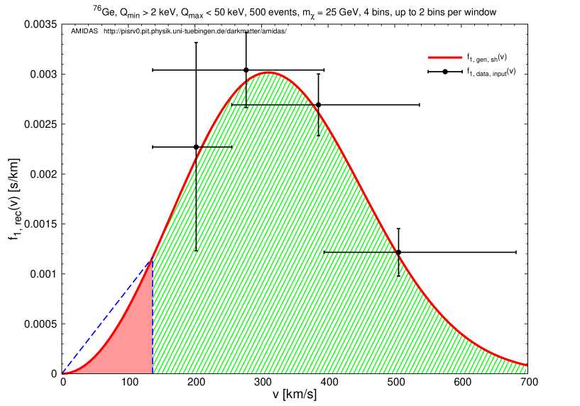
In Fig. 2, we show the reconstructed (rough) velocity distribution (black crosses) with the normalization constant estimated by Eq. (26). The vertical dashed blue line indicates $v_{\rm min}(Q_{\rm min}=2~{}{\rm keV})=136.44$ km/s. Thus the meshed green area above $v_{\rm min}^{\ast}=136.44$ km/s denotes the integral on the left–hand side of the normalization condition (25), whereas the shaded light–red area blow $v_{\rm min}^{\ast}$ has been neglected.

Fig. 2 shows that the reconstructed velocity distribution with the modified normalization constant given by Eq. (26) is strongly improved and could already match the true (input) velocity distribution (the solid red curve) pretty well. However, Fig. 2 shows also clearly that the contribution below the non–zero minimal cut–off velocity $v_{\rm min}^{\ast}$ (the shaded light–red area) would still be non–negligible!

3.2 Contribution below the non–zero minimal cut–off velocity

The reconstructed velocity distribution shown in Fig. 2 matches almost perfectly to the true (input) distribution. However, as pointed out in the previous section, since not only the tiny contribution from the $v>v_{\rm max}$ area ($<0.5\%$) but also a pretty large part from $v\leq v_{\rm min}^{\ast}=136.44$ km/s (the shaded light–red area) has been omitted, the normalization condition (25) with the integral over $f_{1}(v)$ only between $v_{\rm min}^{\ast}$ and $v_{\rm max}$ could be considerably underestimated. Hence, an estimator for the area under the (true) velocity distribution function in the velocity range $[0,v_{\rm min}^{\ast}]$ should be given.

In this section, we suggest a model–independent estimate for the area below $v_{\rm min}^{\ast}$. As sketched in Fig. 2, for this aim, the value of the velocity distribution function at $v=v_{\rm min}^{\ast}$ has to be estimated and we approximate then the area of $v\leq v_{\rm min}^{\ast}$ simply by a triangle. We start with the reconstructed recoil spectrum in the first $Q-$bin which can be given by

$$\left(\frac{dR}{dQ}\right)_{{\rm expt},~{}\!1}=r_{1}~{}\!e^{k_{1}(Q-Q_{s,1})}~{}\!.$$ (27)

By using Eq. (3), an expression, similar to Eq. (11), for the value of the reconstructed velocity distribution function at $v=v_{\rm min}^{\ast}$ can be found as

$$f_{1,{\rm rec}}(v_{\rm min}^{\ast})={\cal N}\Bigg{[}\frac{2Q_{\rm min}r(Q_{\rm min})}{F^{2}(Q_{\rm min})}\Bigg{]}\left[\frac{d}{dQ}\ln F^{2}(Q)\bigg{|}_{Q=Q_{\rm min}}-k_{1}\right]\equiv{\cal N}\tilde{f}_{1,{\rm rec}}(v_{\rm min}^{\ast})~{}\!.$$ (28)

Combining Eqs. (22) and (28), the integral over $f_{1}(v)$ between 0 and $v_{\rm max}^{\ast}$ can be given by

$$\int_{0}^{\infty}f_{1}(v)~{}\!dv \simeq \left(\int_{0}^{v_{\rm min}^{\ast}}+\int_{v_{\rm min}^{\ast}}^{v_{\rm max}}\right)f_{1}(v)~{}\!dv$$ (29)

$$\simeq {\cal N}\tilde{f}_{1,{\rm rec}}(v_{\rm min}^{\ast})\cdot\frac{v_{\rm min}^{\ast}}{2}+{\cal N}\left(\frac{\alpha}{2}\right)\left[\frac{2Q_{\rm min}^{1/2}r(Q_{\rm min})}{F^{2}(Q_{\rm min})}+I_{0}(Q_{\rm min},Q_{\rm max}^{\ast})\right]$$

$$= {\cal N}\left(\frac{\alpha}{2}\right)\left[\tilde{f}_{1,{\rm rec}}(v_{\rm min}^{\ast})\sqrt{Q_{\rm min}}+\frac{2Q_{\rm min}^{1/2}r(Q_{\rm min})}{F^{2}(Q_{\rm min})}+I_{0}(Q_{\rm min},Q_{\rm max}^{\ast})\right]$$

$$= 1~{}\!.$$

Therefore, we can obtain the model–independent approximation for the normalization constant of the reconstructed WIMP velocity distribution as

$${\cal N}=\frac{2}{\alpha}\left[\tilde{f}_{1,{\rm rec}}(v_{\rm min}^{\ast})~{}\!Q_{\rm min}^{1/2}+\frac{2Q_{\rm min}^{1/2}r(Q_{\rm min})}{F^{2}(Q_{\rm min})}+I_{0}(Q_{\rm min},Q_{\rm max}^{\ast})\right]^{-1}~{}\!.$$ (30)

Note that the modified normalization constant ${\cal N}$ given here depends now on the estimates of $r_{1}$ and $k_{1}$. Hence, the covariance matrix of the estimates $f_{1,{\rm rec}}(v_{s,\mu})$ needs to be modified as:

$${\rm cov}\Big{(}f_{1,{\rm rec}}(v_{s,\mu}),f_{1,{\rm rec}}(v_{s,\nu})\Big{)}$$ (31)

$$= \left[\frac{f_{1,{\rm rec}}(v_{s,\mu})f_{1,{\rm rec}}(v_{s,\nu})}{r_{\mu}r_{\nu}}\right]{\rm cov}\left(r_{\mu},r_{\nu}\right)+\left(2{\cal N}\right)^{2}\left[\frac{Q_{s,\mu}Q_{s,\nu}r_{\mu}r_{\nu}}{F^{2}(Q_{s,\mu})F^{2}(Q_{s,\nu})}\right]{\rm cov}\left(k_{\mu},k_{\nu}\right)$$

$$~{}~{}~{}~{}-{\cal N}\left\{\left[\frac{f_{1,{\rm rec}}(v_{s,\mu})}{r_{\mu}}\right]\left[\frac{2Q_{s,\nu}r_{\nu}}{F^{2}(Q_{s,\nu})}\right]{\rm cov}\left(r_{\mu},k_{\nu}\right)+\Big{(}\mu\longleftrightarrow\nu\Big{)}\right\}$$

$$~{}~{}~{}~{}~{}~{}~{}~{}+\left[\frac{\partial f_{1,{\rm rec}}(v_{s,\mu})}{\partial r_{1}}\right]\left[\frac{\partial f_{1,{\rm rec}}(v_{s,\nu})}{\partial r_{1}}\right]\sigma^{2}(r_{1})+\left[\frac{\partial f_{1,{\rm rec}}(v_{s,\mu})}{\partial k_{1}}\right]\left[\frac{\partial f_{1,{\rm rec}}(v_{s,\nu})}{\partial k_{1}}\right]\sigma^{2}(k_{1})$$

$$~{}~{}~{}~{}~{}~{}~{}~{}~{}~{}~{}~{}+\left\{\left[\frac{\partial f_{1,{\rm rec}}(v_{s,\mu})}{\partial r_{1}}\right]\left[\frac{\partial f_{1,{\rm rec}}(v_{s,\nu})}{\partial k_{1}}\right]+\Big{(}\mu\longleftrightarrow\nu\Big{)}\right\}{\rm cov}\left(r_{1},k_{1}\right)$$

$$~{}~{}~{}~{}~{}~{}~{}~{}~{}~{}~{}~{}~{}~{}~{}~{}+\left\{\left[\frac{\partial f_{1,{\rm rec}}(v_{s,\mu})}{\partial r_{1}}\right]\left[\frac{\partial f_{1,{\rm rec}}(v_{s,\nu})}{\partial r_{\nu}}\right]{\rm cov}\left(r_{1},r_{\nu}\right)\right.$$

$$~{}~{}~{}~{}~{}~{}~{}~{}~{}~{}~{}~{}~{}~{}~{}~{}~{}~{}~{}~{}~{}~{}+\left[\frac{\partial f_{1,{\rm rec}}(v_{s,\mu})}{\partial r_{1}}\right]\left[\frac{\partial f_{1,{\rm rec}}(v_{s,\nu})}{\partial k_{\nu}}\right]{\rm cov}\left(r_{1},k_{\nu}\right)$$

$$~{}~{}~{}~{}~{}~{}~{}~{}~{}~{}~{}~{}~{}~{}~{}~{}~{}~{}~{}~{}~{}~{}~{}~{}+\left[\frac{\partial f_{1,{\rm rec}}(v_{s,\mu})}{\partial k_{1}}\right]\left[\frac{\partial f_{1,{\rm rec}}(v_{s,\nu})}{\partial r_{\nu}}\right]{\rm cov}\left(k_{1},r_{\nu}\right)$$

$$~{}~{}~{}~{}~{}~{}~{}~{}~{}~{}~{}~{}~{}~{}~{}~{}~{}~{}~{}~{}~{}~{}~{}~{}~{}~{}+\Bigg{.}\left[\frac{\partial f_{1,{\rm rec}}(v_{s,\mu})}{\partial k_{1}}\right]\left[\frac{\partial f_{1,{\rm rec}}(v_{s,\nu})}{\partial k_{\nu}}\right]{\rm cov}\left(k_{1},k_{\nu}\right)+\Big{(}\mu\longleftrightarrow\nu\Big{)}\Bigg{\}}~{}\!.$$

All derivatives of $f_{1,{\rm rec}}(v_{s,\mu})$ to $r_{1}$, $r_{\mu}$, $k_{1}$ and $k_{\mu}$ needed here are given in Appendix A.2.

Figure 3: The reconstructed (rough) velocity distribution (black crosses) with the normalization constant estimated by Eq. (30) and the modified statistical uncertainties given by Eq. (31). The dotted magenta horizontal lines indicate the reconstructed velocity distributions including the correction of the theoretical estimate of the difference between the triangular approximation and the integral between 0 and $v_{\rm min}^{\ast}$ (see the next section). All parameters are as in Fig. 1.

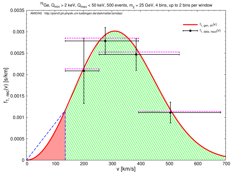
In Fig. 3, we show the reconstructed (rough) velocity distribution (black crosses) with the normalization constant estimated by Eq. (30) and the modified statistical uncertainties given by Eq. (31). It can be found that, due to the contribution of the first term in the bracket in Eq. (30), the reconstructed velocity distribution points are now a little bit underestimated. Meanwhile, the statistical uncertainties (vertical bars) given by Eq. (31) becomes now a bit larger, except the first one, which is significantly reduced.

Figure 4: As in Figs. 2 (upper) and 3 (lower), except that the experimental threshold energy has been increased to $Q_{\rm min}=5$ keV. Note that the vertical scale of $f_{1,{\rm rec}}(v)$ is different here.

Figure 5: As in Figs. 4, except that ${}^{28}{\rm Si}$ is used as the target nucleus. Note that the vertical scale of $f_{1,{\rm rec}}(v)$ is different here.

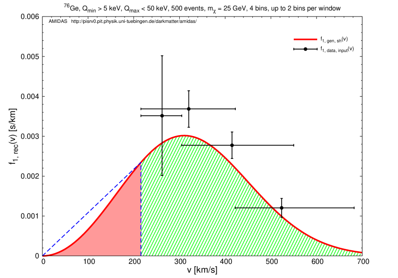
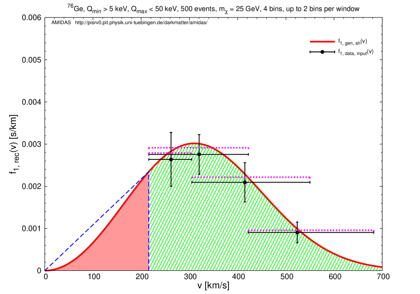
As a stricter check of our model–independent modification of the normalization constant ${\cal N}$, in Figs. 4, we increase the experimental threshold energy to $Q_{\rm min}=5$ keV. For a germanium detector, the corresponding minimal cut–off velocity of the incident WIMPs is now 215.72 km/s and thus the contribution from the area of $v\leq v_{\rm min}^{\ast}$ becomes much larger. Hence, the underestimate of the normalization constant given by Eq. (26) and in turn the overestimate of the reconstructed velocity distribution points are more clear. In contrast, by using Eq. (30) the reconstructed points can still match the true (input) velocity distribution pretty well. However, and more importantly, the systematic bias between the triangular approximation and the real value of the integral of the $v\leq v_{\rm min}^{\ast}$ area becomes more obviously and problematic. We will discuss this drawback in more details in the next section.

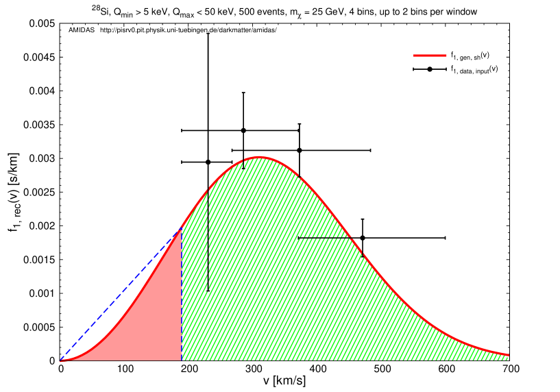
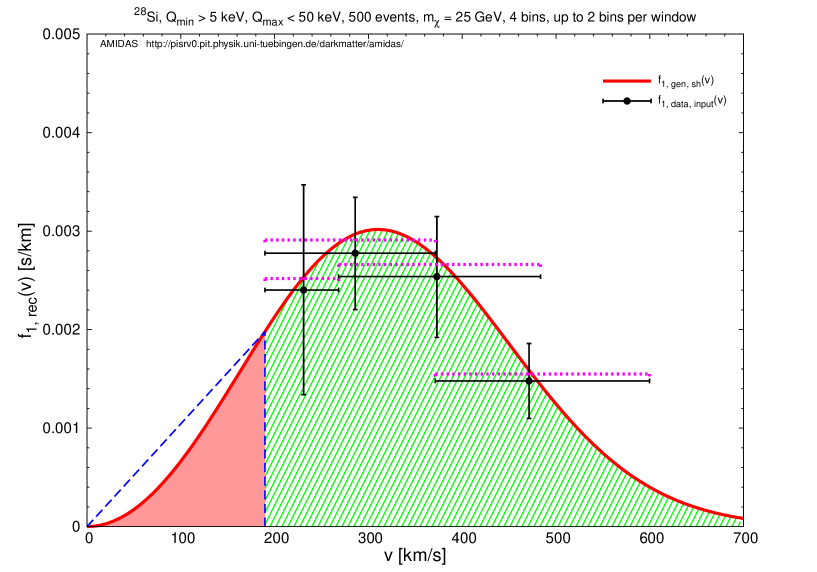
Finally, in Figs. 5, a lighter target nucleus ${}^{28}{\rm Si}$ is used as the detector material. For a silicon detector with an experimental threshold energy of 5 keV, the corresponding minimal cut–off velocity of the incident WIMPs is 189.64 km/s. As the case with a ${}^{76}{\rm Ge}$ target, the estimator (30) for the normalization constant ${\cal N}$ combined with the modified covariance matrix given in Eq. (31) can not only correct the overestimated reconstructed velocity distribution very well, but also strongly reduce the large statistical uncertainty on the first reconstructed distribution point $f_{1,{\rm rec}}(v_{s,1})$, although the statistical uncertainties are (a bit) larger than those given with the Ge target (cf. Figs. 4).

3.3 Bias of the estimator (30) for the normalization constant ${\cal N}$

As revealed in Figs. 2 to 5, our model–independent triangular estimator for the integral over $f_{1}(v)$ between 0 and $v_{\rm min}^{\ast}$ is somehow overestimated. Then the normalization constant ${\cal N}$ and the reconstructed velocity distribution points are in turn (a bit) underestimated. In this section, we discuss therefore the bias of the estimator (30) for the normalization constant ${\cal N}$ in more details.

$v_{\rm min}^{\ast}$ [km/s]	$Q_{\rm min}$ [keV]				$\frac{\Delta_{0}^{v_{\rm min}^{\ast}}}{\int_{0}^{v_{\rm min}^{\ast}}f_{1}(v)~{}\!dv}$	$\frac{\Delta_{0}^{v_{\rm min}^{\ast}}-\int_{0}^{v_{\rm min}^{\ast}}f_{1}(v)~{}\!dv}{\int_{0}^{v_{\rm max}}f_{1}(v)~{}\!dv}$  [%]
	${}^{28}{\rm Si}$	${}^{40}{\rm Ar}$	${}^{76}{\rm Ge}$	${}^{136}{\rm Xe}$
10	0.014	0.013	0.011	0.008	1.4997	0.0012
20	0.056	0.054	0.043	0.031	1.4987	0.0094
30	0.125	0.120	0.097	0.069	1.4970	0.0315
40	0.222	0.214	0.172	0.123	1.4946	0.0742
50	0.348	0.334	0.269	0.192	1.4916	0.1435
60	0.500	0.482	0.387	0.276	1.4877	0.2452
70	0.681	0.655	0.526	0.376	1.4830	0.3839
80	0.890	0.856	0.688	0.491	1.4775	0.5635
90	1.126	1.083	0.870	0.621	1.4711	0.7868
100	1.390	1.338	1.074	0.767	1.4637	1.0551
120	2.002	1.926	1.547	1.105	1.4458	1.7246
140	2.725	2.622	2.106	1.504	1.4234	2.5495
160	3.560	3.424	2.750	1.964	1.3960	3.4757
180	4.504	4.334	3.481	2.486	1.3634	4.4152
200	5.561	5.350	4.298	3.069	1.3253	5.2473
220	6.729	6.474	5.200	3.713	1.2816	5.8242
240	8.008	7.705	6.189	4.419	1.2323	5.9807
260	9.398	9.042	7.263	5.186	1.1777	5.5473
280	10.900	10.487	8.423	6.015	1.1180	4.3668
300	12.512	12.039	9.670	6.905	1.0537	2.3101

Table 1: The theoretically estimated ratios of the triangular approximation (to the integral over $f_{1}(v)$ in the range between 0 and $v_{\rm min}^{\ast}$) to the integral itself as well as the fractions of the difference between the triangular approximation and the integral between 0 and $v_{\rm min}^{\ast}$ (i.e. the little overestimated amount) to the integral in the entire velocity range between 0 and $v_{\rm max}$. The most commonly used model for the Galactic WIMP velocity distribution function, $f_{1,{\rm sh}}(v)$ given in Eq. (19), has been used. 20 different values of $v_{\rm min}^{\ast}$ from 10 to 300 km/s for four most commonly used detector materials are given here. The $Q_{\rm min}$ values have been estimated for the WIMP mass of $m_{\chi}=25$ GeV.

Taking the most commonly used shifted Maxwellian velocity distribution $f_{1,{\rm sh}}(v)$ given in Eq. (19) as our theoretical assumption, in Table 1 we give the estimated ratios of the triangular approximation (to the integral over $f_{1}(v)$ in the range between 0 and $v_{\rm min}^{\ast}$) to the integral itself:

$$\frac{\Delta_{0}^{v_{\rm min}^{\ast}}}{\int_{0}^{v_{\rm min}^{\ast}}f_{1}(v)~{}\!dv}~{}\!,$$ (32)

as well as the fractions of the difference between the triangular approximation and the integral between 0 and $v_{\rm min}^{\ast}$ (i.e. the little overestimated amount) to the integral in the entire velocity range between 0 and $v_{\rm max}$:

$$\frac{\Delta_{0}^{v_{\rm min}^{\ast}}-\int_{0}^{v_{\rm min}^{\ast}}f_{1}(v)~{}\!dv}{\int_{0}^{v_{\rm max}}f_{1}(v)~{}\!dv}~{}\!.$$ (33)

20 different values of $v_{\rm min}^{\ast}$ from 10 to 300 km/s for four most commonly used detector materials are given.

As references, in Figs. 3 to 5 the reconstructed velocity distributions taking into account the corrections of the theoretical estimate of the difference between the triangular approximation and the integral over $f_{1}(v)$ between 0 and $v_{\rm min}^{\ast}$, $\Delta_{0}^{v_{\rm min}^{\ast}}-\int_{0}^{v_{\rm min}^{\ast}}f_{1}(v)~{}\!dv$, have also been given as the dotted magenta horizontal lines. It can then be seen clearly that, with this (final) model–dependent correction for the normalization constant ${\cal N}$, the reconstructed velocity distributions could match the true (input) distribution function very precisely: The tiny differences would totally be negligible, compared to the much larger statistical uncertainties given with ${\cal O}(500)$ WIMP events.

Note however that, giving the correction of the systematic bias requires a theoretically predicted velocity distribution function. For practical use without prior knowledge about the one–dimensional WIMP velocity distribution as well as for improving the simple triangular approximation to the integral of the $v\leq v_{\rm min}^{\ast}$ area (depending on the estimate of $f_{1}(v)$ at $v=v_{\rm min}^{\ast}$), one could use an iterative procedure with the Bayesian reconstructed velocity distribution function [6]. Nevertheless, considering the pretty large statistical uncertainties on the reconstructed velocity distribution points as well as the much narrower statistical uncertainty band of the Bayesian reconstructed velocity distribution [6], the effect of ignoring the much smaller systematic bias with or even without the model–dependent theoretical corrections could not be significant (at least in the next few years).

Figure 6: The theoretically estimated fraction of the difference between the triangular approximation and the integral over $f_{1}(v)$ between 0 and $v_{\rm min}^{\ast}$ (i.e. the little overestimated amount) to the integral in the entire velocity range between 0 and $v_{\rm max}$ as a function of $v_{\rm min}^{\ast}$.

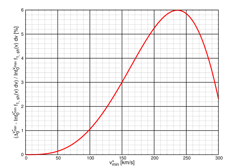
Besides of Table 1, in Fig. 6 we give the theoretically estimated fraction of the difference between the triangular approximation and the integral over $f_{1}(v)$ between 0 and $v_{\rm min}^{\ast}$ (i.e. the little overestimated amount) to the integral in the entire velocity range between 0 and $v_{\rm max}$ as a function of $v_{\rm min}^{\ast}$ for reader’s reference.

4 Summary and conclusions

In this paper, we investigated the modification of our expressions developed for the model–independent data analysis procedure of the reconstruction of the (time–averaged) one–dimensional velocity distribution of Galactic WIMPs with a non–negligible experimental threshold energy.

It our earlier work [5], the experimental maximal and minimal cut–off energies have been assumed to be large or small enough. Thus the sum over all recorded events in the data set can be used as the estimator for the integral over the one–dimensional WIMP velocity distribution function, which is in turn needed for the estimation of the normalization constant of the reconstructed velocity distribution. For experiments with heavy target nuclei, e.g. Ge or Xe, and once WIMPs are heavy ($\>\raisebox{-3.01385pt}{$\stackrel{{\scriptstyle\textstyle>}}{{\sim}}$}\>~{}100$ GeV), the systematic bias caused by this assumption should be acceptable. However, once WIMPs are light ($\>\raisebox{-3.01385pt}{$\stackrel{{\scriptstyle\textstyle<}}{{\sim}}$}\>~{}50$ GeV) and a light target nucleus, e.g. Si or Ar, is used for reconstructing the WIMP velocity distribution $f_{1}(v)$, effects of a non–negligible threshold energy has to be considered and the estimate of the normalization constant of $f_{1}(v)$ would need in turn to be modified properly.

In this work, we derived at first the expression for estimating the integral over $f_{1}(v)$ between the minimal and maximal reconstructable velocities. Then we suggested the simple model–independent triangular approximation to the contribution below the minimal reconstructable velocity. Finally, by adopting the most commonly used shifted Maxiwellian velocity distribution function, the correction of the systematic bias caused by the use of the simple triangular approximation has been given. Our numerical simulations presented in this paper show that, for a minimal reconstructable velocity of as high as ${\cal O}(200)$ km/s, our model–independent modification of the estimator for the normalization constant (with or even without the model–dependent correction of the systematic bias) could provide precise reconstructed velocity distribution points to match the true WIMP velocity distribution with a  $\stackrel{{\scriptstyle\textstyle<}}{{\sim}}$  10% bias.

In summary, as a supplement of our earlier works on the (Bayesian) reconstruction of the WIMP velocity distribution function, we developed in this paper a model–independent modification of the estimator for the normalization constant of $f_{1}(v)$ for the more general case with a non–negligible experimental threshold energy. This modification should not only be more suitable for our Bayesian reconstruction of the one–dimensional WIMP velocity distribution function [6], but hopefully also offer preciser information about Galactic Dark Matter for direct and indirect detection experiments and phenomenology.

Acknowledgments

The author would like to thank the Physikalisches Institut der Universität Tübingen for the technical support of the computational work presented in this paper. This work was partially supported by the CAS Fellowship for Taiwan Youth Visiting Scholars under the grant no. 2013TW2JA0002 as well as the Department of Human Resources and Social Security of Xinjiang Uygur Autonomous Region.

Appendix A Formulae for estimating statistical uncertainties

Here we list all formulae needed for the model–independent method for the reconstruction of the one–dimensional WIMP velocity distribution function described in Sec. 2 as well as for the modification of the normalization constant ${\cal N}$ by Eq. (30) and the modified covariance matrix of the estimates of $f_{1,{\rm rec}}(v_{s,n})$. Detailed derivations and discussions can be found in Ref. [5].

A.1 Formulae needed in Sec. 2

First, by using the standard Gaussian error propagation, the expressions for the uncertainties on the standard estimator $r_{n}$ and the logarithmic slope $k_{n}$ estimated by Eq. (8) can be given directly as

$$\sigma^{2}(r_{n})=\frac{N_{n}}{b_{n}^{2}}~{}\!,$$ (A1)

and

$$\sigma^{2}(k_{n})=k_{n}^{4}\left\{1-\left[\frac{k_{n}b_{n}/2}{\sinh(k_{n}b_{n}/2)}\right]^{2}\right\}^{-2}\sigma^{2}\left(\overline{Q-Q_{n}}|_{n}\right)~{}\!,$$ (A2)

where

$$\sigma^{2}\left(\overline{Q-Q_{n}}|_{n}\right)=\frac{1}{N_{n}-1}\bigg{[}\overline{(Q-Q_{n})^{2}}|_{n}-\overline{Q-Q_{n}}|_{n}^{2}\bigg{]}~{}\!.$$ (A3)

For replacing the “bin” quantities by “window” quantities, one needs the covariance matrix for $\overline{Q-Q_{\mu}}|_{\mu}$, which follows directly from the definition (16):

$${\rm cov}\left(\overline{Q-Q_{\mu}}|_{\mu},\overline{Q-Q_{\nu}}|_{\nu}\right)$$ (A4)

$$= \frac{1}{N_{\mu}N_{\nu}}\sum_{n=n_{\nu-}}^{n_{\mu+}}\bigg{[}N_{n}\left(\overline{Q}|_{n}-\overline{Q}|_{\mu}\right)\left(\overline{Q}|_{n}-\overline{Q}|_{\nu}\right)+N_{n}^{2}\sigma^{2}\left(\overline{Q-Q_{n}}|_{n}\right)\bigg{]}~{}\!.$$

Note that, firstly, $\mu\leq\nu$ has been assumed here and the covariance matrix is, of course, symmetric. Secondly, the sum is understood to vanish if the two windows $\mu$, $\nu$ do not overlap, i.e. if $n_{\mu+}<n_{\nu-}$. Moreover, similar to Eq. (A1), we can get

$${\rm cov}(r_{\mu},r_{\nu})=\frac{1}{w_{\mu}w_{\nu}}\sum_{n=n_{\nu-}}^{n_{\mu+}}N_{n}~{}\!,$$ (A5)

where $\mu\leq\nu$ has again been taken. And the mixed covariance matrix can be given by

$${\rm cov}\left(r_{\mu},\overline{Q-Q_{\nu}}|_{\nu}\right)=\frac{1}{w_{\mu}N_{\nu}}\sum_{n=n_{-}}^{n_{+}}N_{n}\left(\overline{Q}|_{n}-\overline{Q}|_{\nu}\right)~{}\!.$$ (A6)

Note here that this sub–matrix is not symmetric under the exchange of $\mu$ and $\nu$. In the definition of $n_{-}$ and $n_{+}$ we therefore have to distinguish two cases:

$$\begin{array}[]{l c l}n_{-}=n_{\nu-},~{}n_{+}=n_{\mu+},&{}{}{}{}{}{}{}{}{}{}{}{}\hfil&{\rm if}~{}\mu\leq\nu~{}\!;\\ n_{-}=n_{\mu-},~{}n_{+}=n_{\nu+},&&{\rm if}~{}\mu\geq\nu~{}\!.\end{array}$$ (A9)

As before, the sum in Eq. (A6) is understood to vanish if $n_{-}>n_{+}$.

Furthermore, the covariance matrices involving the estimators of the logarithmic slopes $k_{\mu}$, estimated by Eq. (8) with replacing $n\to\mu$, can be given from Eq. (A2) as

$${\rm cov}\left(k_{\mu},k_{\nu}\right) = k_{\mu}^{2}k_{\nu}^{2}\left\{1-\left[\frac{k_{\mu}b_{\mu}/2}{\sinh(k_{\mu}b_{\mu}/2)}\right]^{2}\right\}^{-1}\left\{1-\left[\frac{k_{\nu}b_{\nu}/2}{\sinh(k_{\nu}b_{\nu}/2)}\right]^{2}\right\}^{-1}$$ (A10)

$$~{}~{}~{}~{}~{}~{}~{}~{}~{}~{}~{}~{}~{}~{}~{}~{}\times{\rm cov}\left(\overline{Q-Q_{\mu}}|_{\mu},\overline{Q-Q_{\nu}}|_{\nu}\right)~{}\!,$$

and

$${\rm cov}\left(r_{\mu},k_{\nu}\right)=k_{\nu}^{2}\left\{1-\left[\frac{k_{\nu}b_{\nu}/2}{\sinh(k_{\nu}b_{\nu}/2)}\right]^{2}\right\}^{-1}{\rm cov}\left(r_{\mu},\overline{Q-Q_{\nu}}|_{\nu}\right)~{}\!.$$ (A11)

A.2 Derivatives of the modified estimates $f_{1,{\rm rec}}(v_{s,\mu})$

The modified normalization constant ${\cal N}$ given by Eq. (30) depends on the estimates of $r_{1}$ and $k_{1}$, as the first reconstructed point of the velocity distribution given in Eq. (11), $f_{1,{\rm rec}}(v_{s,1})$. For modifying the covariance matrix of the estimates of $f_{1}(v)$, one needs thus to distinguish the $\mu=1$ case from the other $\mu\neq 1$ cases.

First, for the general $\mu\neq 1$ case, one has

$$f_{1,{\rm rec}}(v_{s,\mu}) = \frac{2}{\alpha}\left[\tilde{f}_{1,{\rm rec}}(v_{\rm min}^{\ast})~{}\!Q_{\rm min}^{1/2}+\frac{2Q_{\rm min}^{1/2}r(Q_{\rm min})}{F^{2}(Q_{\rm min})}+I_{0}(Q_{\rm min},Q_{\rm max}^{\ast})\right]^{-1}$$ (A12)

$$~{}~{}~{}~{}~{}~{}~{}~{}~{}~{}~{}~{}\times\Bigg{[}\frac{2Q_{s,\mu}r_{\mu}}{F^{2}(Q_{s,\mu})}\Bigg{]}\left[\frac{d}{dQ}\ln F^{2}(Q)\bigg{|}_{Q=Q_{s,\mu}}-k_{\mu}\right]$$

$$= \frac{2}{\alpha}\left\{\Bigg{[}\frac{2Q_{\rm min}^{1/2}r_{1}e^{k_{1}(Q_{\rm min}-Q_{s,1})}}{F^{2}(Q_{\rm min})}\Bigg{]}\left\{\left[\frac{d}{dQ}\ln F^{2}(Q)\bigg{|}_{Q=Q_{\rm min}}-k_{1}\right]Q_{\rm min}+1\right\}\right.$$

$$~{}~{}~{}~{}~{}~{}~{}~{}~{}~{}~{}~{}~{}~{}~{}~{}~{}~{}~{}~{}~{}~{}~{}~{}\Bigg{.}+I_{0}(Q_{\rm min},Q_{\rm max}^{\ast})\Bigg{\}}^{-1}$$

$$~{}~{}~{}~{}~{}~{}~{}~{}~{}~{}~{}~{}\times\Bigg{[}\frac{2Q_{s,\mu}r_{\mu}}{F^{2}(Q_{s,\mu})}\Bigg{]}\left[\frac{d}{dQ}\ln F^{2}(Q)\bigg{|}_{Q=Q_{s,\mu}}-k_{\mu}\right]~{}\!.$$

Then the derivative of $f_{1,{\rm rec}}(v_{s,\mu})$ to $r_{1}$ can be given as

$$\frac{\partial f_{1,{\rm rec}}(v_{s,\mu})}{\partial r_{1}} = -\frac{2}{\alpha}\bigg{\{}\cdots\bigg{\}}^{-2}\Bigg{[}\frac{2Q_{\rm min}^{1/2}e^{k_{1}(Q_{\rm min}-Q_{s,1})}}{F^{2}(Q_{\rm min})}\Bigg{]}\left\{\left[\frac{d}{dQ}\ln F^{2}(Q)\bigg{|}_{Q=Q_{\rm min}}-k_{1}\right]Q_{\rm min}+1\right\}$$ (A13a)

$$~{}~{}~{}~{}~{}~{}~{}~{}~{}~{}~{}~{}\times\Bigg{[}\frac{2Q_{s,\mu}r_{\mu}}{F^{2}(Q_{s,\mu})}\Bigg{]}\left[\frac{d}{dQ}\ln F^{2}(Q)\bigg{|}_{Q=Q_{s,\mu}}-k_{\mu}\right]$$

$$= -\frac{f_{1,{\rm rec}}(v_{s,\mu})}{r_{1}}\left[1-{\cal N}\left(\frac{\alpha}{2}\right)I_{0}(Q_{\rm min},Q_{\rm max}^{\ast})\right]~{}\!.$$

And the derivative of $f_{1,{\rm rec}}(v_{s,\mu})$ to $k_{1}$ is

$$\frac{\partial f_{1,{\rm rec}}(v_{s,\mu})}{\partial k_{1}} = -\frac{2}{\alpha}\bigg{\{}\cdots\bigg{\}}^{-2}\Bigg{[}\frac{2Q_{\rm min}^{1/2}r_{1}e^{k_{1}(Q_{\rm min}-Q_{s,1})}}{F^{2}(Q_{\rm min})}\Bigg{]}$$ (A13b)

$$~{}~{}~{}~{}~{}~{}\times\left\{\left(Q_{\rm min}-Q_{s,1}\right)\left\{\left[\frac{d}{dQ}\ln F^{2}(Q)\bigg{|}_{Q=Q_{\rm min}}-k_{1}\right]Q_{\rm min}+1\right\}-Q_{\rm min}\right\}$$

$$~{}~{}~{}~{}~{}~{}~{}~{}~{}~{}~{}~{}\times\Bigg{[}\frac{2Q_{s,\mu}r_{\mu}}{F^{2}(Q_{s,\mu})}\Bigg{]}\left[\frac{d}{dQ}\ln F^{2}(Q)\bigg{|}_{Q=Q_{s,\mu}}-k_{\mu}\right]$$

$$= -f_{1,{\rm rec}}(v_{s,\mu})\left[{\cal N}\left(\frac{\alpha}{2}\right)\right]\Bigg{[}\frac{2Q_{\rm min}^{1/2}r(Q_{\rm min})}{F^{2}(Q_{\rm min})}\Bigg{]}$$

$$~{}~{}~{}~{}~{}~{}\times\left\{\left(Q_{\rm min}-Q_{s,1}\right)\left[\frac{d}{dQ}\ln F^{2}(Q)\bigg{|}_{Q=Q_{\rm min}}-k_{1}\right]Q_{\rm min}-Q_{s,1}\right\}~{}\!.$$

Note that once $Q_{\rm min}=0$, the second term in the bracket in the second line of Eq. (A13a) reduces to 1 and $\partial f_{1,{\rm rec}}(v_{s,\mu})/\partial r_{1}$ as well as $\partial f_{1,{\rm rec}}(v_{s,\mu})/\partial k_{1}$ become 0. Moreover, similar to the calculations done for the covariance matrix in Eq. (17), one can get

$$\frac{\partial f_{1,{\rm rec}}(v_{s,\mu})}{\partial r_{\mu}}=\frac{f_{1,{\rm rec}}(v_{s,\mu})}{r_{\mu}}~{}\!,$$ (A14a)

and

$$\frac{\partial f_{1,{\rm rec}}(v_{s,\mu})}{\partial k_{\mu}}=-{\cal N}\Bigg{[}\frac{2Q_{s,\mu}r_{\mu}}{F^{2}(Q_{s,\mu})}\Bigg{]}~{}\!.$$ (A14b)

On the other hand, for the special $\mu=1$ case, we have

$$f_{1,{\rm rec}}(v_{s,1}) = \frac{2}{\alpha}\left\{\Bigg{[}\frac{2Q_{\rm min}^{1/2}r_{1}e^{k_{1}(Q_{\rm min}-Q_{s,1})}}{F^{2}(Q_{\rm min})}\Bigg{]}\left\{\left[\frac{d}{dQ}\ln F^{2}(Q)\bigg{|}_{Q=Q_{\rm min}}-k_{1}\right]Q_{\rm min}+1\right\}\right.$$ (A15)

$$~{}~{}~{}~{}~{}~{}~{}~{}~{}~{}~{}~{}~{}~{}~{}~{}~{}~{}~{}~{}~{}~{}~{}~{}\Bigg{.}+I_{0}(Q_{\rm min},Q_{\rm max}^{\ast})\Bigg{\}}^{-1}$$

$$~{}~{}~{}~{}~{}~{}~{}~{}~{}~{}~{}~{}\times\Bigg{[}\frac{2Q_{s,1}r_{1}}{F^{2}(Q_{s,1})}\Bigg{]}\left[\frac{d}{dQ}\ln F^{2}(Q)\bigg{|}_{Q=Q_{s,1}}-k_{1}\right]~{}\!.$$

Then, similar to the calculations done in Eqs. (A13a) to (A14b), it can be found that

$$\frac{\partial f_{1,{\rm rec}}(v_{s,1})}{\partial r_{1}}=\left.\frac{\partial f_{1,{\rm rec}}(v_{s,\mu})}{\partial r_{1}}\right|_{\mu=1}+\left.\frac{\partial f_{1,{\rm rec}}(v_{s,\mu})}{\partial r_{\mu}}\right|_{\mu=1}~{}\!,$$ (A16a)

and

$$\frac{\partial f_{1,{\rm rec}}(v_{s,1})}{\partial k_{1}}=\left.\frac{\partial f_{1,{\rm rec}}(v_{s,\mu})}{\partial k_{1}}\right|_{\mu=1}+\left.\frac{\partial f_{1,{\rm rec}}(v_{s,\mu})}{\partial k_{\mu}}\right|_{\mu=1}~{}\!.$$ (A16b)

References

- [1] G. Jungman, M. Kamionkowski and K. Griest, “Supersymmetric Dark Matter”, Phys. Rep. 267, 195–373 (1996), arXiv:hep-ph/9506380.
- [2] M. Drees and G. Gerbier, “Mini–Review of Dark Matter: 2012”, updated minireview for “The Review of Particle Physics 2012”, arXiv:1204.2373 [hep-ph] (2012).
- [3] L. E. Strigari, “Galactic Searches for Dark Matter”, Phys. Rep. 531, 1–88 (2013), arXiv:1211.7090 [astro-ph.CO].
- [4] L. Baudis, “Direct Dark Matter Detection: the Next Decade”, Issue on “The Next Decade in Dark Matter and Dark Energy”, Phys. Dark Univ. 1, 94–108 (2012), arXiv:1211.7222 [astro-ph.IM].
- [5] M. Drees and C.-L. Shan, “Reconstructing the Velocity Distribution of Weakly Interacting Massive Particles from Direct Dark Matter Detection Data”, J. Cosmol. Astropart. Phys. 0706, 011 (2007), arXiv:astro-ph/0703651.
- [6] C.-L. Shan, “Bayesian Reconstruction of the Velocity Distribution of Weakly Interacting Massive Particles from Direct Dark Matter Detection Data”, J. Cosmol. Astropart. Phys. 1408, 009 (2014), arXiv:1403.5610 [astro-ph.HE].
- [7] M. Drees and C.-L. Shan, “Model–Independent Determination of the WIMP Mass from Direct Dark Matter Detection Data”, J. Cosmol. Astropart. Phys. 0806, 012 (2008), arXiv:0803.4477 [hep-ph].
- [8] K. Freese, J. Frieman and A. Gould, “Signal Modulation in Cold–Dark–Matter Detection”, Phys. Rev. D37, 3388–3405 (1988).
-
[9]
C.-L. Shan,
the AMIDAS (A Model–Independent Data Analysis System)
package and website for direct Dark Matter detection experiments and phenomenology,
http://pisrv0.pit.physik.uni-tuebingen.de/darkmatter/amidas/ (2009);
the mirror website on TiResearch (Taiwan interactive Research),
http://www.tir.tw/phys/hep/dm/amidas/. - [10] C.-L. Shan, “AMIDAS-II: Upgrade of the AMIDAS Package and Website for Direct Dark Matter Detection Experiments and Phenomenology”, Phys. Dark Univ. 5–6, 240–306 (2014), arXiv:1403.5611 [astro-ph.IM].
- [11] M. Lisanti, L. E. Strigari, J. G. Wacker and R. H. Wechsler, “The Dark Matter at the End of the Galaxy”, Phys. Rev. D 83, 023519 (2011), arXiv:1010.4300 [astro-ph.CO].
[12]
Y.-Y. Mao, L. E. Strigari, R. H. Wechsler, H.-Y. Wu and O. Hahn,
“Halo–to–Halo Similarity and Scatter in the Velocity Distribution of Dark Matter”
Astrophys. J. 764, 35 (2013),
arXiv:1210.2721 [astro-ph.CO];
Y.-Y. Mao, L. E. Strigari and R. H. Wechsler, “Connecting Direct Dark Matter Detection Experiments to Cosmologically Motivated Halo Models”, Phys. Rev. D 89, 063513 (2014), arXiv:1304.6401 [astro-ph.CO]. - [13] M. Kuhlen, A. Pillepich, J. Guedes and P. Madau, “The Distribution of Dark Matter in the Milky Way’s Disk”, Astrophys. J. 784, 161 (2014), arXiv:1308.1703 [astro-ph.GA].