Isotropic inverse-problem approach for two-dimensional phase unwrapping

Abstract

In this paper, we propose a new technique for two-dimensional phase unwrapping. The unwrapped phase is found as the solution of an inverse problem that consists in the minimization of an energy functional. The latter includes a weighted data-fidelity term that favors sparsity in the error between the true and wrapped phase differences, as well as a regularizer based on higher-order total-variation. One desirable feature of our method is its rotation invariance, which allows it to unwrap a much larger class of images compared to the state of the art. We demonstrate the effectiveness of our method through several experiments on simulated and real data obtained through the tomographic phase microscope. The proposed method can enhance the applicability and outreach of techniques that rely on quantitative phase evaluation.

1 Introduction

Two-dimensional phase unwrapping is an essential component in a majority of techniques used for quantitative phase imaging. A typical example of standard application is tomographic phase microscopy [CFYB⁺07], where the phase of the transmitted wave-field must be first unwrapped before being interpreted as a line integral of the refractive index along the direction of propagation. Phase unwrapping is also used for estimation of terrain elevation in synthetic aperture radar [RHJ⁺00], wave/fat separation in magnetic resonance imaging [SNPG95], and estimation of wave-front distortion in adaptive optics [Fri77]. Accordingly, improvements in phase unwrapping methodology can enhance the applicability and outreach of techniques that rely on quantitative phase evaluation.

The centrality of phase unwrapping has resulted in the development of many practical solutions to the problem. Such solutions include direct approaches based on path-following such as the two-dimensional extension of the well known Itoh’s method [Ito82] as well as more evolved strategies based on branch cuts [GZW88] or quality maps [HBLG02]. The current trend in the literature is to formulate the task of phase unwrapping as an inverse problem in a path-independent way. Earlier works have proposed to minimize the quadratic error between the true and wrapped phase differences [Hun79, TT88, GR94]. Marroquin and Rivera [MR95] have applied Tikhonov regularization to improve and stabilize the performance of the least-squares approach. They showed that the introduction of the regularization term permits the algorithm to cope with noise and missing data. Huang et al. [HTZ⁺12] showed that the performance of phase unwrapping is further improved when replacing Tikhonov with total-variation regularization. In the context of phase unwrapping, Ghiglia and Romero [GR96] recognized the tendency of quadratic-penalty to smooth image edges and proposed to minimize a more general $\ell_{p}$ norm–based criterion as an alternative. They found that the performance of phase unwrapping improves when $0\leq p\leq 1$, albeit at the increase in computational cost. Similarly, Rivera and Marroquin [RM04] have investigated nonconvex optimization strategies relying on half-quadratic regularization. More recently, González and Jacques [GJ14] have proposed an iterative unwrapping method based on $\ell_{1}$ minimization that additionally promotes sparsity of the solution in the wavelet domain. Ying et al. [YLJ⁺06] have proposed an iterative method based on dynamic programming that models the phase as a Markov random field. Bioucas-Dias and Valadão [BDV07] have proposed an energy functional based on generalized $\ell_{p}$ norm and corresponding minimization algorithm that relies on graph-cut methods. Their PUMA algorithm in its original form and its noise tolerant extensions [BDKAE08, VBD09] are currently considered state of the art. Mei et al. [MKCG13] have proposed an application specific method that jointly unwraps and denoises time-of-flight phase images using a message-passing algorithm. An extended review of this topic, along with related algorithmic ideas, can be found in the book [GP98] and tutorial [Yin06].

In this paper, we propose a new variational-reconstruction approach for phase unwrapping that is robust to noise. In particular, our aim is to improve on state of the art by introducing an improved energy functional and demonstrating its benefits. The main contributions of this paper can be summarized as follows:

• Formulation of the unwrapping as an optimization problem where the data-fidelity term penalizes the weighted $\ell_{1}$-norm of the error in a way that is invariant to rotations. Our formulation thus allows the phase image to contain edges that are of arbitrary orientation, which is distinct from traditional approaches in literature [GR96, RM04, YLJ⁺06, BDV07, GJ14].

• Use of a non-quadratic regularization term that allows our method to cope with noise, while still preserving sharp edges in the phase image. Our regularizer consists of a higher-order extension of total-variation (TV) that is currently considered state of the art in the context of resolution of linear inverse problems in biomedical imaging [LWU13].

• Design of a novel iterative algorithm for phase unwrapping. The algorithm approximates the minimum $\ell_{0}$-norm solution by solving a sequence of weighted $\ell_{1}$-norm minimization problems, where the weights at the next iteration are computed from the value of the current solution. Since our energy functional is non-smooth, we rely on a well known alternating direction method of multipliers (ADMM) [BPC⁺11] to decompose the minimization into a sequence of simpler operations.

This paper is organized as follows. In Section 2, we introduce our formulation of the phase unwrapping, and discuss the relevance of this new approach for obtaining high-quality solutions in practice. In Section 3, we derive our reconstruction algorithm. In Section 4, we conduct experiments on simulated and real phase unwrapping problems, and compare our method with the state of the art from both qualitative and quantitative standpoints. We summarize and conclude our work in Section 5.

2 Problem formulation

We consider the following observation model

$$\bm{\psi}=\mathcal{W}\left(\bm{\phi}\right)=\bm{\phi}-2\pi\bm{k}$$ (1)

where $\bm{k}\in\mathbb{Z}^{N}$ and $\bm{\phi},\bm{\psi}\in\mathbb{R}^{N}$. The vectors $\bm{\psi}$ and $\bm{\phi}$ represent vectorized versions of the wrapped and unwrapped phase images, respectively. The wrapping is represented by a component-wise function $\mathcal{W}$ that is defined as

$$\mathcal{W}(\phi)\,\triangleq\,\left[\left(\left(\phi+\pi\right)\mod 2\pi\right)-\pi\right]\quad\in\quad\left[-\pi,\pi\right).$$

When noise is part of the measurements, we assume that the unwrapped phase vector $\bm{\phi}$ in our model represents the noisy version of the true phase $\bm{\varphi}$.

Generally, the two-dimensional phase unwrapping problem is ill-posed. However, it can be solved exactly in the noiseless scenario, when the phase $\bm{\phi}$ satisfies the two-dimensional extension of Itoh’s continuity condition [Ito82]. Let $\mathbf{D}:\mathbb{R}^{N}\rightarrow\mathbb{R}^{N\times 2}$ denote the discrete counterpart of the gradient operator and let

$$\mathbf{D}\bm{\phi}=\begin{bmatrix}\mathbf{D}_{x}\bm{\phi}\\[3.00003pt] \mathbf{D}_{y}\bm{\phi}\end{bmatrix},$$ (2)

where $\mathbf{D}_{x}$ and $\mathbf{D}_{y}$ denote the finite-difference operator along the horizontal and vertical directions, respectively. If, for a given pixel $n\in[1,\dots,N]$, the unwrapped phase $\bm{\phi}$ satisfies

$$\|[\mathbf{D}\bm{\phi}]_{n}\|_{\ell_{2}}\,\triangleq\,\sqrt{([\mathbf{D}_{x}\bm{\phi}]_{n})^{2}+([\mathbf{D}_{y}\bm{\phi}]_{n})^{2}}\leq\pi,$$ (3)

then, we have the equality

$$[\mathbf{D}\bm{\phi}]_{n}=\mathcal{W}([\mathbf{D}\bm{\psi}]_{n}).$$ (4)

Here, $[\mathbf{D}\bm{\phi}]_{n}\,\triangleq\,([\mathbf{D}_{x}\bm{\phi}]_{n},[\mathbf{D}_{y}\bm{\phi}]_{n})$ denotes the $n$-th component of the gradient $\mathbf{D}\bm{\phi}$. Relation (4) suggests that two-dimensional phase unwrapping may be accomplished by a simple phase summation, provided that (3) is satisfied at all pixels $n$. Note that the formulation in (3) imposes the Itoh’s continuity condition on both gradient components simultaneously due to the norm inequality

$$\max\left(\left|a\right|,\left|b\right|\right)\leq\sqrt{a^{2}+b^{2}},$$

which holds for any $a,b\in\mathbb{R}$.

In practice, however, condition (3) will not be fulfilled at all pixel locations due to the presence of sharp edges and of measurement noise. Yet, it can still be expected to hold for the great majority of pixels of the unwrapped phase image. We thus formulate phase unwrapping as the following minimization problem

$$\widehat{\bm{\phi}}=\mathop{\mathrm{arg\,min}}_{\bm{\phi}\in\bm{\Phi}}\left\{\mathcal{D}(\bm{\phi})+\tau\mathcal{R}(\bm{\phi})\right\},$$ (5)

where $\mathcal{D}$ is the data-fidelity term and $\mathcal{R}$ is the regularization term, to be discussed shortly. The convex set $\bm{\Phi}=\{\bm{\phi}\in\mathbb{R}^{N}\,:\,\phi_{1}=\psi_{1}\}\subset\mathbb{R}^{N}$ enforces the first pixel of the solution $\bm{\phi}$ to match the first pixel of the wrapped phase $\bm{\psi}$, which removes the additive constant ambiguity present in phase unwrapping. The parameter $\tau>0$ controls the amount of regularization.

The data-fidelity term in (5) is given by

$$\mathcal{D}(\bm{\phi})\,\triangleq\,\sum_{n=1}^{N}w_{n}\|[\mathbf{D}\bm{\phi}-\mathcal{W}(\mathbf{D}\bm{\psi})]_{n}\|_{\ell_{2}},$$ (6)

where $\bm{w}\in\mathbb{R}_{+}^{N}$ are positive weights. It is intended to relax the strict equality (4).

In the unweighted case, i.e. when $w_{n}=1$ for all $n\in[1,\dots,N]$, $\mathcal{D}$ corresponds to $\ell_{1}$-norm penalty on the magnitudes of $\bm{\epsilon}\,\triangleq\,\mathbf{D}\bm{\phi}-\mathcal{W}(\mathbf{D}\bm{\psi})$. It can be interpreted as a convex relaxation of $\ell_{0}$-norm penalty that enforces sparse magnitudes of $\bm{\epsilon}$. This implies that our data-term favors $\bm{\phi}$ whose gradient $\mathbf{D}\bm{\phi}$ agrees with $\mathcal{W}(\mathbf{D}\bm{\psi})$ on most of the pixels. Moreover, our data-fidelity term $\mathcal{D}$ penalizes both horizontal $\bm{\epsilon}_{x}$ and vertical $\bm{\epsilon}_{y}$ components of $\bm{\epsilon}$ in a joint fashion. This is significantly different from traditional formulations in the literature [GR96, GJ14], where the $\ell_{1}$-norm is penalized in a separable fashion as $\|\bm{\epsilon}\|_{\ell_{1}}=\|\bm{\epsilon}_{x}\|_{\ell_{1}}+\|\bm{\epsilon}_{y}\|_{\ell_{1}}$. In fact, there is a clear analogy between our formulation (6) and the isotropic, i.e. rotation invariant, form of total-variation (TV) that is often used for edge-preserving image restoration [BT09]. Similarly, the separable $\ell_{1}$-penalty $\|\bm{\epsilon}\|_{\ell_{1}}$ is analogous to the anisotropic form of TV. The arbitrary orientation of edges in a typical image makes isotropic TV penalty a preferred choice for image restoration. The numerical experiments presented in Sec. 4 illustrate that indeed our method based on isotropic formulation can unwrap a larger class of images compared to other state-of-the-art phase unwrapping methods.

It has been reported in several works [GR96, BDV07] that nonconvex approaches based on $\ell_{p}$-norm penalization of $\bm{\epsilon}$, with $0\leq p<1$, further improve the performance of phase unwrapping. In particular, $\ell_{0}$-norm is generally accepted as the most desirable in practice. One of the properties of $\ell_{1}$-norm that distinguishes it from $\ell_{0}$ is that it takes into account the actual values of the magnitudes of $\bm{\epsilon}$, whereas $\ell_{0}$-norm disregards this information and only counts the support. One possible strategy for selecting weights in the context of $\ell_{1}$ minimization proposed by Candès et al. [CWB08] is to pick $\bm{w}$ such that it counteracts the influence of the magnitude on the $\ell_{1}$-norm. For example, suppose that the weights were inversely proportional to the true magnitudes

$$w_{n}=\begin{cases}\frac{1}{\|[\bm{\epsilon}]_{n}\|_{\ell_{2}}}&\text{if }\|[\bm{\epsilon}]_{n}\|_{\ell_{2}}\neq 0\\ \infty&\text{if }\|[\bm{\epsilon}]_{n}\|_{\ell_{2}}=0.\end{cases}$$ (7)

Then, if there are exactly $m$ pixels violating (3), the minimizer in (5) is guaranteed to find the solution corresponding to $\ell_{0}$ data-fidelity term. The large values in $\bm{w}$ force the solution $\widehat{\bm{\phi}}$ to concentrate on the pixels where the weights are small, and by construction these correspond precisely to the pixels where the magnitudes of $\bm{\epsilon}$ are nonzero. Typically, these pixels correspond to the area of the phase image that contains a sharp edge. It is clearly impossible to construct the precise weights (7) without knowing the unwrapped phase $\bm{\phi}$ itself, but this suggests more generally that large weights could be used to discourage nonzero magnitudes in $\bm{\epsilon}$, while small weights could be used to encourage nonzero magnitudes in $\bm{\epsilon}$.

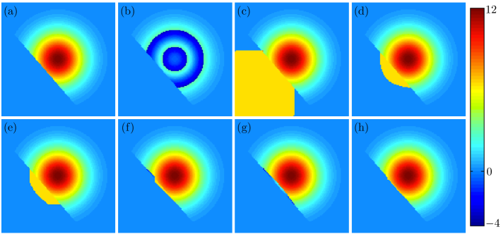
Figure 1: Phase unwrapping of $128\times 128$ image of a truncated Gaussian function. (a) true phase, (b) wrapped phase, (c) Goldstein’s algorithm (GA), (d) least-squares (LS), (e) iteratively reweighted LS (IRLS), (f) PUMA, (g) proposed method with uniform weights, (h) proposed method with adaptive weights (IRTV).

As regularization term in (5), we propose to use the Schatten norms of the Hessian matrix at every pixel of the image [LWU13]. Specifically, we set

$$\mathcal{R}(\bm{\phi}) \,\triangleq\,\|\mathbf{H}\bm{\phi}\|_{1,\mathcal{S}_{1}}$$ (8a)

$$\,\triangleq\,\sum_{n=1}^{N}(\sigma_{1}([\mathbf{H}\bm{\phi}]_{n})+\sigma_{2}([\mathbf{H}\bm{\phi}]_{n})),$$ (8b)

where $\mathbf{H}:\mathbb{R}^{N}\rightarrow\mathbb{R}^{N\times 2\times 2}$ is the discrete Hessian operator and $\|\mathbf{H}\bm{\phi}\|_{1,\mathcal{S}_{1}}$ is the nuclear norm that is computed by summing singular values $\sigma_{1}([\mathbf{H}\bm{\phi}]_{n})$ and $\sigma_{2}([\mathbf{H}\bm{\phi}]_{n})$ of the Hessian matrix at position $n$. There are four major advantages of using such Hessian Schatten-norm (HS) regularization:

• As a higher order regularizer HS avoids the staircase effect of TV and results in piecewise-smooth variations of intensity in the reconstructed phase image. Accordingly, this makes HS particularly well suited for biological and medical specimens that consist of complicated structures such as filaments.

• Similarly to the data-fidelity term $\mathcal{D}$, our regularizer $\mathcal{R}$ is convex and rotation invariant [LWU13]. Rotation invariance implies that we can expect it to work equally well on phase images that contain objects of arbitrary orientations.

• HS regularization has been shown to be state of the art in resolution of linear inverse problems. In particular, it was shown in [LWU13] that HS consistently outperforms other popular regularizers such as Tikhonov, wavelet, and TV.

• Convexity and its algebraic structure make HS amenable to efficient algorithmic implementation and thus practical for large scale inverse problems that are typical in imaging.

To demonstrate the performance of our variational approach (5), we present a phase unwrapping experiment on a synthetic image consisting of a 2D Gaussian function of amplitude $12$ and standard deviation $20$ that has been truncated along a line of arbitrary orientation (here about $40^{\textrm{o}}$). Fig. 1 illustrates the results for four standard unwrapping methods such as Goldstein’s algorithm (GA) [GZW88], least-squares (LS) [GR94], iteratively reweighted LS (IRLS) with data-dependent weights that approximate the $\ell_{0}$-norm penalty [GR96], and PUMA [BDV07]. We additionally illustrate the performance of our method with the emphasis on the influence of weights $\bm{w}$ over the final solution $\widehat{\bm{\phi}}$. Accordingly, we show the solution of (5) with uniform and data-dependent weights. As expected, all algorithms perform equally well in the continuous region of the image. On the other hand, our approach is the only one that accurately captures the discontinuous region of the unwrapped image. This is expected due to rotation invariance of our energy functional. Additionally, we note that the LS method, which is also based on rotation invariant energy functional, fails to preserve the edge due to excessive smoothing. Finally, a careful inspection of Figs. 1 (g) and (h) reveals that the edge is much sharper when the weights $\bm{w}$ are selected in a data-dependent fashion as explained next in Sec. 3.

3 Reconstruction algorithm

We now describe our computational approach based on the convex optimization problem (5). The iterative scheme alternates between estimating $\bm{\phi}$ and redefining the weights $\bm{w}$ as follows.

1. Initialization: Set iteration number to $t=1$. Select an initial phase $\bm{\phi}^{0}\in\mathbb{R}^{N}$ and set $w_{n}^{0}=1$ for each $n=1,\dots,N$.

2. Optimization: For a fixed $\bm{w}^{t-1}$, compute the phase image $\bm{\phi}^{t}$ by solving (5). Also, compute the auxiliary variable $\bm{\epsilon}^{t}=\mathbf{D}\bm{\phi}^{t}-\mathcal{W}(\mathbf{D}\bm{\psi})$.

3. Weight adaptation: For each $n=1,\dots,N$

   $$w_{n}^{t}=\begin{cases}\frac{1}{\|[\bm{\epsilon}^{t}]_{n}\|_{\ell_{2}}}&\text{if }\epsilon_{\textrm{min}}\leq\|[\bm{\epsilon}^{t}]_{n}\|_{\ell_{2}}\leq\epsilon_{\textrm{max}}\\ \frac{1}{\epsilon_{\textrm{max}}}&\text{if }\|[\bm{\epsilon}^{t}]_{n}\|_{\ell_{2}}\geq\epsilon_{\textrm{max}}\\ \frac{1}{\epsilon_{\textrm{min}}}&\text{if }\|[\bm{\epsilon}^{t}]_{n}\|_{\ell_{2}}\leq\epsilon_{\textrm{min}}\\ \end{cases}$$ (9)

4. Stop on convergence or when $t$ attains a specific maximum number of iterations $t_{\textrm{max}}$. Otherwise, increment $t$ and proceed to step 2.

The two parameters $\epsilon_{\textrm{min}}$ and $\epsilon_{\textrm{max}}$ in step 3 provide stability and avoid divisions by zero. For our experiments in Sec 4, we set $\epsilon_{\textrm{max}}=1/\epsilon_{\textrm{min}}=10$. The optimization in step 2 will be discussed shortly.

Although the initial phase $\bm{\phi}^{0}$ can be set to an arbitrary vector in $\mathbb{R}^{N}$, in practice, a warm initialization leads to a smaller number of iterations required for convergence, and hence faster unwrapping times. In our experiments, we found that the solution of LS can serve as a computationally inexpensive way of obtaining a good initialization.

Using an adaptive approach to construct the weights progressively improves the unwrapping around the discontinuities in the phase image. These phase discontinuities might be due to a presence of a sharp edge or due to strong noise. Even though the early phase estimate may be inaccurate, the largest coefficients of $\bm{\epsilon}$ are most likely to be identified with a phase discontinuity. Once these locations are identified, their influence is downweighted in order to gain in sensitivity for identifying the remaining regions of the phase image.

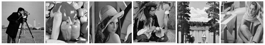
Figure 2: Set of standard test images. From left to right: Cameraman, Peppers, Lena, Man, Lake, and Barbara.

Table 1: Performance of the five considered phase unwrapping methods in terms of SNR on the set of standard test images for various amplitudes

Img/Amp		SNR (dB)
		GA	LS	IRLS	PUMA	IRTV
Cameraman	4	33.99	38.76	32.74	35.72	$\bm{\infty}$
	5	23.38	25.79	24.07	23.89	25.65
	6	14.10	15.51	19.06	17.41	19.98
	7	-1.31	7.57	15.64	12.73	16.09
	8	0.00	2.35	0.38	0.73	0.92
	9	1.63	2.64	2.02	1.90	2.17
Peppers	4	$\bm{\infty}$	$\bm{\infty}$	$\bm{\infty}$	$\bm{\infty}$	$\bm{\infty}$
	5	36.69	$\bm{\infty}$	$\bm{\infty}$	$\bm{\infty}$	$\bm{\infty}$
	6	23.64	22.60	$\bm{\infty}$	$\bm{\infty}$	$\bm{\infty}$
	7	14.40	11.67	$\bm{\infty}$	26.39	$\bm{\infty}$
	8	7.27	8.23	23.96	14.93	27.62
	9	5.58	3.97	15.69	15.64	15.75
Lena	4	$\bm{\infty}$	$\bm{\infty}$	$\bm{\infty}$	$\bm{\infty}$	$\bm{\infty}$
	5	$\bm{\infty}$	$\bm{\infty}$	$\bm{\infty}$	$\bm{\infty}$	$\bm{\infty}$
	6	38.56	27.77	$\bm{\infty}$	$\bm{\infty}$	$\bm{\infty}$
	7	23.62	18.70	$\bm{\infty}$	$\bm{\infty}$	$\bm{\infty}$
	8	12.20	13.33	36.29	30.30	$\bm{\infty}$
	9	-2.97	7.33	25.50	15.51	30.47

Img/Amp		SNR (dB)
		GA	LS	IRLS	PUMA	IRTV
Man	4	$\bm{\infty}$	$\bm{\infty}$	$\bm{\infty}$	$\bm{\infty}$	$\bm{\infty}$
	5	26.29	32.31	$\bm{\infty}$	$\bm{\infty}$	$\bm{\infty}$
	6	10.12	24.55	30.47	29.43	$\bm{\infty}$
	7	11.70	18.14	24.23	27.46	29.22
	8	8.75	10.17	21.89	12.08	25.26
	9	6.95	6.75	12.69	8.36	13.23
Lake	4	$\bm{\infty}$	$\bm{\infty}$	$\bm{\infty}$	$\bm{\infty}$	$\bm{\infty}$
	5	$\bm{\infty}$	$\bm{\infty}$	$\bm{\infty}$	$\bm{\infty}$	$\bm{\infty}$
	6	40.10	$\bm{\infty}$	$\bm{\infty}$	$\bm{\infty}$	$\bm{\infty}$
	7	26.62	25.21	$\bm{\infty}$	41.44	$\bm{\infty}$
	8	15.99	13.84	18.02	17.69	18.10
	9	-0.88	2.84	15.91	15.33	16.52
Barbara	4	$\bm{\infty}$	$\bm{\infty}$	$\bm{\infty}$	$\bm{\infty}$	$\bm{\infty}$
	5	$\bm{\infty}$	$\bm{\infty}$	$\bm{\infty}$	$\bm{\infty}$	$\bm{\infty}$
	6	$\bm{\infty}$	$\bm{\infty}$	$\bm{\infty}$	$\bm{\infty}$	$\bm{\infty}$
	7	43.54	40.53	$\bm{\infty}$	$\bm{\infty}$	$\bm{\infty}$
	8	35.60	30.07	44.70	$\bm{\infty}$	$\bm{\infty}$
	9	31.01	22.01	$\bm{\infty}$	45.72	$\bm{\infty}$

Table 2: Phase unwrapping results for the noisy Man image of size $128\times 128$ and amplitude $a=6$.

Method / Input SNR	16 dB	18 dB	20 dB
GA	14.40	19.03	18.72
LS	23.57	25.75	27.97
PUMA	31.13	31.96	34.96
IRTV $(\tau=0)$	28.13	30.21	34.96
IRTV $(\tau=10^{-3})$	28.52	31.97	$\bm{\infty}$
IRTV $(\tau=10^{-2})$	35.02	34.98	$\bm{\infty}$
IRTV $(\tau=10^{-1})$	18.86	24.56	28.46

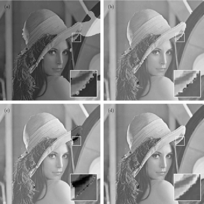
Figure 3: Phase unwrapping results for Lena image of size $256\times 256$ when the amplitude is $a=9$. (a) LS (SNR = 7.33 dB); (b) IRLS (SNR = 25.50 dB); (c) PUMA (SNR = 15.51 dB); (d) IRTV (SNR = 30.47 dB).

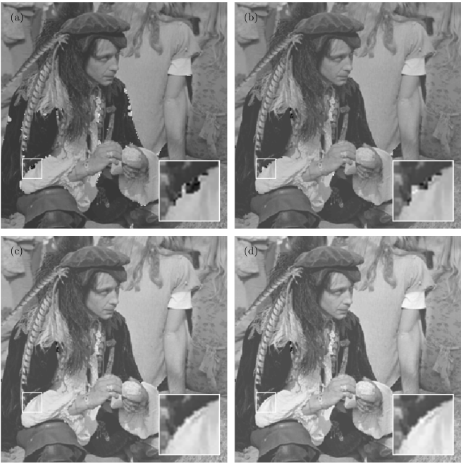
Figure 4: Phase unwrapping results for Man image of size $256\times 256$ when the amplitude is $a=7$. (a) LS (SNR = 18.14 dB); (b) IRLS (SNR = 24.23 dB); (c) PUMA (SNR = 27.46 dB); (d) IRTV (SNR = 29.22 dB).

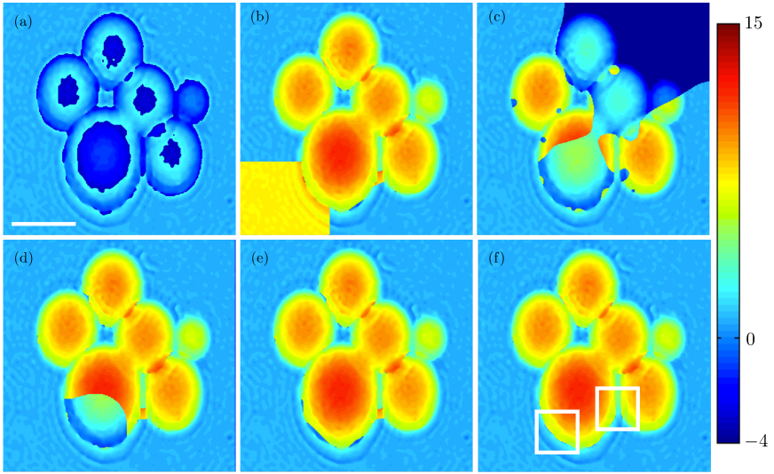
Figure 5: Phase unwrapping results for Beads image of size $512\times 512$ obtained from the phase of the transmitted field. (a) wrapped phase; (b) GA; (c) LS; (d) IRLS; (e) PUMA; (f) IRTV. Scale bar, 5 $\mu$m.

The step 2 of the algorithm requires the resolution of the non-smooth optimization problem (5). We perform this minimization by designing an augmented-Lagrangian (AL) scheme [NW06]. Specifically, we seek the critical points of the following AL

$$\mathcal{L} (\bm{\phi},\bm{\epsilon},\bm{s})\,\triangleq\,\sum_{n=1}^{N}w_{n}\|[\bm{\epsilon}]_{n}\|_{\ell_{2}}+\tau\mathcal{R}(\bm{\phi})$$

$$\hskip 10.00002pt+\bm{s}^{T}\left(\bm{\epsilon}-\mathbf{D}\bm{\phi}+\bm{d}\right)+\frac{\rho}{2}\|\bm{\epsilon}-\mathbf{D}\bm{\phi}+\bm{d}\|_{\ell_{2}}^{2}$$

$$=\frac{\rho}{2}\left\|\bm{\epsilon}-\mathbf{D}\bm{\phi}+\bm{d}+\frac{\bm{s}}{\rho}\right\|_{\ell_{2}}^{2}$$

$$\hskip 10.00002pt+\sum_{n=1}^{N}w_{n}\|[\bm{\epsilon}]_{n}\|_{\ell_{2}}+\tau\mathcal{R}(\bm{\phi})-\frac{1}{2\rho}\|\bm{s}\|_{\ell_{2}}^{2},$$

where $\bm{d}\,\triangleq\,\mathcal{W}(\mathbf{D}\bm{\psi})$ is the data vector, $\bm{s}\in\mathbb{R}^{N\times 2}$ is the dual variable that imposes the constraint $\bm{\epsilon}=\mathbf{D}\bm{\phi}-\bm{d}$, and $\rho>0$ is the quadratic penalty parameter. Traditionally, an AL scheme solves the problem (5) by alternating between a joint minimization step and an update step as

$$(\bm{\phi}^{k},\bm{\epsilon}^{k}) \leftarrow\mathop{\mathrm{arg\,min}}_{\bm{\phi}\in\bm{\Phi},\;\bm{\epsilon}\in\mathbb{R}^{N\times 2}}\left\{\mathcal{L}(\bm{\phi},\bm{\epsilon},\bm{s}^{k-1})\right\}$$ (10a)

$$\bm{s}^{k} \leftarrow\bm{s}^{k-1}+\rho(\bm{\epsilon}^{k}-\mathbf{D}\bm{\phi}^{k}+\bm{d}).$$ (10b)

However, the joint minimization step (10a) can be computationally intensive. To circumvent this problem, we separate (10a) into a succession of simpler steps. This form of separation is commonly known as alternating direction method of multipliers (ADMM) [BPC⁺11] and can be described as follows

$$\bm{\phi}^{k} \leftarrow\mathop{\mathrm{arg\,min}}_{\bm{\phi}\in\bm{\Phi}}\left\{\mathcal{L}(\bm{\phi},\bm{\epsilon}^{k-1},\bm{s}^{k-1})\right\}$$ (11a)

$$\bm{\epsilon}^{k} \leftarrow\mathop{\mathrm{arg\,min}}_{\bm{\epsilon}\in\mathbb{R}^{N\times 2}}\left\{\mathcal{L}(\bm{\phi}^{k},\bm{\epsilon},\bm{s}^{k-1})\right\}$$ (11b)

$$\bm{s}^{k} \leftarrow\bm{s}^{k-1}+\rho(\bm{\epsilon}^{k}-\mathbf{D}\bm{\phi}^{k}+\bm{d}).$$ (11c)

By ignoring the terms that do not depend on $\bm{\phi}$, the step (11a) can be expressed as

$$\bm{\phi}^{k}\leftarrow\mathop{\mathrm{arg\,min}}_{\bm{\phi}\in\bm{\Phi}}\left\{\frac{1}{2}\left\|\mathbf{D}\bm{\phi}-\bm{z}^{k-1}\right\|_{\ell_{2}}^{2}+\frac{\tau}{\rho}\mathcal{R}(\bm{\phi})\right\},$$ (12)

with $\bm{z}^{k-1}\,\triangleq\,\bm{\epsilon}^{k-1}+\bm{d}+\bm{s}^{k-1}/\rho$. This step corresponds to a classical Hessian Schatten–regularized linear inverse problem. The solution of this problem can be efficiently solved with the publicly available software that has been described in [LWU13]. Similarly, the step (11b) can be simplified as follows

$$\bm{\epsilon}^{k}\leftarrow\mathop{\mathrm{arg\,min}}_{\bm{\epsilon}\in\mathbb{R}^{N\times 2}}\left\{\frac{\rho}{2}\left\|\bm{\epsilon}-\bm{y}^{k}\right\|_{\ell_{2}}^{2}+\sum_{n=1}^{N}w_{n}\|[\bm{\epsilon}]_{n}\|_{\ell_{2}}\right\},$$

with $\bm{y}^{k}\,\triangleq\,\mathbf{D}\bm{\phi}^{k}-\bm{d}-\bm{s}^{k-1}/\rho$. This step is solved directly by component-wise application of the following shrinkage function

$$\mathcal{T}(\bm{y};\tau) \,\triangleq\,\mathop{\mathrm{arg\,min}}_{\bm{x}\in\mathbb{R}^{2}}\left\{\frac{1}{2}\|\bm{x}-\bm{y}\|_{\ell_{2}}^{2}+\tau\|\bm{x}\|_{\ell_{2}}\right\}$$

$$=\max\left(\|\bm{y}\|_{\ell_{2}}-\tau,0\right)\frac{\bm{y}}{\|\bm{y}\|_{\ell_{2}}}.$$

Thus, we can express (11b) as

$$[\bm{\epsilon}^{k}]_{n}\leftarrow\mathcal{T}\left(\left[\mathbf{D}\bm{\phi}^{k}-\bm{d}-\bm{s}^{k-1}/\rho\right]_{n};w_{n}/\rho\right),$$

for every $n=1,\dots,N$.

While the theoretical convergence of our algorithm requires the full convergence of ADMM inner iterations (11), in practice, we found that, by using a sufficiently high number of iterations $k_{\textrm{max}}$ with an additional stopping criterion, our algorithm achieves excellent results as illustrated in Sec. 4. In particular, we implemented the standard criterion suggested by Boyd et al. [BPC⁺11], where ADMM is stopped when then primal and dual residuals are small

$$\|\bm{\epsilon}^{k}-\mathbf{D}\bm{\phi}^{k}-\bm{d}\|_{\ell_{2}}\leq\delta_{\textrm{inner}}$$ (13a)

$$\|\rho\mathbf{D}(\bm{\phi}^{k}-\bm{\phi}^{k-1})\|_{\ell_{2}}\leq\delta_{\textrm{inner}},$$ (13b)

where the constant $\delta_{\textrm{inner}}>0$ controls the desired inner tolerance level. In all our experiments, we set $\delta_{\textrm{inner}}=10^{-2}$ and $k_{\textrm{max}}=2000$.

For outer iterations, our algorithm relies on a separate number of $t_{\textrm{max}}$ iterations with a distinct stopping criterion based on measuring the relative change of the solution in two successive iterations as

$$\frac{\|\bm{\phi}^{t}-\bm{\phi}^{t-1}\|_{\ell_{2}}}{\|\bm{\phi}^{t-1}\|_{\ell_{2}}}\leq\delta_{\textrm{outer}},$$ (14)

where $\delta_{\textrm{outer}}>0$ controls the desired outer tolerance level. In the experiments, these constants were set to $t_{\textrm{max}}=10$ and $\delta_{\textrm{outer}}=10^{-2}$.

It is important to note that the solution of our iterative method is not consistent in the sense that the rewrapped phase $\mathcal{W}(\widehat{\bm{\phi}})$ is not necessarily equal to the measured phase $\bm{\psi}$. The possible inconsistency of our solution comes from the fact that we are using a continuous optimization for solving an inherently discrete optimization problem (i.e., addition and subtraction of integer multiples of $2\pi$). Accordingly, any method relying on continuous optimization such as LS, IRLS, or the method proposed here, may result in an inconsistent solution. Path-following methods such as Goldstein’s algorithm or discrete optimization algorithms such as PUMA always return consistent solutions. Consistency, however, is easily achieved with a single post-processing step that was proposed by Pritt [Pri97] as

$$\widehat{\bm{\phi}}^{\prime}\leftarrow\widehat{\bm{\phi}}+\mathcal{W}(\bm{\psi}-\widehat{\bm{\phi}}),$$ (15)

where $\widehat{\bm{\phi}}^{\prime}$ is consistent with the wrapped phase $\bm{\psi}$. In the sequel, we perform a single application of the operator (15) to the outputs returned by the continuous optimization algorithms to make their solutions consistent with the measurements.

To conclude, we described a method for minimizing the proposed objective functional. While this forces us to revert to a more costly iterative scheme (instead of finding the solution directly), it allows us to obtain a variational formulation that incorporates the most efficient ideas that have appeared for phrase unwrapping and the stabilization of ill-posed inverse problems. The optimization itself is performed iteratively by relying on ADMM to reduce the problem to a succession of straightforward operations. The final computational time required to unwrap a given image depends on the total number of iterations, which in turn depends on the severity of wrapping. For example, it took us about 3 minutes to unwrap the Gaussian signal in Fig. 1 with a MATLAB implementation of our algorithm running on an iMac using a 4 GHz Intel Core i7 processor. In Section 4, we illustrate that the improvement in reconstruction quality can be rather substantial. We thus believe that the method should be of interest to practitioners that rely on quantitative phase evaluation.

4 Experiments

Based on the above developments, we report the results of our phase unwrapping method in simulated and practical configurations. In particular, we compare the results of our approach, which we shall denote IRTV, against those obtained by using four alternative methods; namely, Golstein’s algorithm (GA) [GZW88], least-squares (LS) [GR94], iterative reweighed LS approach (IRLS) with data-dependent weights that approximate the $\ell_{0}$-norm penalty [GR96], and PUMA [BDV07]. An implementation of PUMA is freely available at http://www.lx.it.pt/~bioucas/code.htm. Mirroring examples provided by the authors of PUMA, we use it with a nonconvex quantized potential of exponent $p=0.5$ where quadratic region threshold is set to $0.5$. As suggested in the PUMA code, we use cliques of higher order by considering $4$ displacement vectors $(1,0),(0.1),(1,1)$ and $(-1,1)$.

In the sequel, a first set of experiments with simulated phase wrapping evaluates the algorithms quantitatively by using the true phase $\bm{\phi}$ for comparison. The experiments that follow allow to determine the relevance of our approach on real data in the context of tomographic phase microscopy.

4.1 Synthetic Data

In this set of experiments, we use a set of $6$ grayscale $256\times 256$ shown in Fig. 2 from the USC-SIPI database at http://sipi.usc.edu/database/. After normalization of its amplitude to $[0,a]$, with $a\in[4,5,6,7,8,9]$, each image is used to generate a distinct wrapped phase image according to our observation model (1). As image amplitude $a$ increases, the edges in the true phase $\bm{\phi}$ become sharper, thus making the unwrapping task increasingly more difficult.

Given the wrapped phase image $\bm{\psi}$, our goal is to determine how accurately the true phase $\bm{\phi}$ can be reconstructed by the standard and proposed methods. As reconstruction parameters, our algorithm uses $\tau=10^{-2}$ and $\epsilon_{\textrm{max}}=1/\epsilon_{\textrm{min}}=10$ in all synthetic experiments. As mentioned before, we set the number of outer and inner iterations to $t_{\textrm{max}}=10$ and $k_{\textrm{max}}=2000$, respectively, with additional stopping criteria (13) and (14). We also use $10$ iterations for finding the solution of Hessian Schatten-regularized inverse problem (12). In principle, the positive scalar $\rho$ of ADMM can either be fixed to some predetermined value or adapted according to the distance to the constraint via the scheme described in [BPC⁺11]. In all our experiments, we used adaptive $\rho$; however, we found that in practice fixed values of $\rho=0.1$ and $\rho=1$ work equally well. Iterative algorithms IRLS and IRTV were initialized with the LS solution. Upon convergence, the solutions of all the variational algorithms were made consistent with a single application of the operator (15).

In Table 1, we report the signal-to-noise ratio $\textrm{SNR (dB)}\,\triangleq\,10\log_{10}\left(\|\bm{\phi}\|_{\ell_{2}}^{2}/\|\bm{\phi}-\widehat{\bm{\phi}}\|_{\ell_{2}}^{2}\right)$ of the unwrapped phase for all the methods considered. When the SNR is more that $300$ dB, we consider the unwrapping to be exact and set the corresponding value in the table to infinity. As can be seen from the table, our method, which is labeled IRTV, consistently provides better reconstruction results for nearly all images and all amplitude values. Specifically, our method successfully unwraps of Cameraman, Lena, and Man phase images for which all other standard methods fail. Note that for Cameraman at amplitudes 5, 8, and 9 LS yields unwrapped phase images of higher quality. While for $a=5$ the difference between LS and IRTV is modest (less that 0.15 dB), for $a=8$ and $a=9$ all the methods completely fail at unwrapping (SNRs below 3 dB).

Beyond the SNR comparisons, the effectiveness of the proposed method can also be visually appreciated by inspecting the more difficult scenarios of Lena and Man images presented in Fig. 3 and Fig. 4. From these examples we can verify our initial claim: our phase unwrapping method recovers oriented sharp edges more accurately than other algorithms thus providing an overall boost in performance.

In order to illustrate the robustness of IRTV to noise, we now consider a simple scenario where the unwrapped phase $\bm{\phi}$ corresponds to a noisy version of the true phase $\bm{\varphi}$. Specifically, we consider the additive noise model $\bm{\phi}=\bm{\varphi}+\bm{e}$, where $\bm{e}$ is additive white Gaussian noise (AWGN). Given the wrapped image $\bm{\psi}=\mathcal{W}(\bm{\phi})=\mathcal{W}(\bm{\varphi}+\bm{e})$, we would like to determine how accurately one can recover $\bm{\phi}$ in the presence of high levels of noise. Noisy phase images are typically more difficult to unwrap due to additional discontinuities that appear across the whole image. Note that robustness to noise is different from denoising, which implies that we do not attempt to reduce the level of noise during the unwrapping process. When unwrapping is successful, one can then denoise the unwrapped image with any state-of-the-art image denoising algorithm suitable to the noise at hand.

In Table 2, we report the SNR of the the estimate $\widehat{\bm{\phi}}$ with respect to the unwrapped phase $\bm{\phi}$ for GA, LS, PUMA, and IRTV algorithms. The true phase $\bm{\varphi}$ is the Man image of amplitude $a=6$ and dimension $128\times 128$. The phase image $\bm{\phi}$ is obtained by adding AWGN of variance corresponding to 16, 18, and 20 dB of $\textrm{input SNR (dB)}\,\triangleq\,10\log_{10}\left(\|\bm{\varphi}\|_{\ell_{2}}^{2}/\|\bm{\phi}-\bm{\varphi}\|_{\ell_{2}}^{2}\right)$. The table presents the median SNR for $10$ independent realizations of the noise. In this example, the average running time of our MATLAB implementation of IRTV was about 7.5 minutes on our iMac using a 4 GHz Intel Core i7 processor. Additionally, the table presents the results of IRTV with different values of regularization parameter $\tau$. Specifically, we report the results for $\tau\in[0,10^{-3},10^{-2},10^{-1}]$. Higher levels of $\tau$ imply stronger regularization during the reconstruction. The results in the table illustrate the advantage of using the Schatten norm of the Hessian to complement our data-fidelity term, i.e., one obtains a significant boost in unwrapping performance when $\tau>0$. Moreover, the influence of $\tau$ grows as the level of noise increases from 20 to 16 dB of input SNR. One must however note that similar to other regularization schemes, there is no theoretically optimal way of setting $\tau$ and its optimal value might depend on the image, amount of wrapping, and noise. Our simulations indicate that the optimal value of $\tau$ lies in the range $[10^{-3},10^{-1}]$ for the configurations considered.

4.2 Real Data

In this second experimental part, we consider phase images that are acquired practically from distinct physical objects. In particular, we consider the setup for tomographic phase microscopy [CFYB⁺07], which is a promising quantitative phase imaging technique. It is based on the principle that, for near-plane wave illumination of a sample, the phase of the transmitted field can be well approximated as the integral of the refractive index along the path of beam propagation. However, for the approximation to hold, the phases extracted from the transmitted fields must be first unwrapped, which significantly limits the applications of the technique for imaging objects that are off-focus, large, or have high index contrast. Once unwrapped, the phase image can simply be interpreted as the projection of refractive index, analogous to the projection of absorption in X-ray tomography.

To evaluate our phase unwrapping algorithm, we measured refractive index tomograms of 6 polystyrene spheres (catalog no. 17135, Polysciences, refractive index $n=1.602$ at 561 nm) immersed in oil with a lower refractive index of 1.516. The wrapped phase image of size $512\times 512$ is extracted from the transmitted field at angle $39.02^{\textrm{o}}$ with respect to vertical axis. This phase data is difficult to unwrap due of numerous visible phase discontinuities that appear along the borders of the beads.

The parameters of our IRTV method were chosen as in the synthetic experiments above with the exception of the regularization parameter that was set to $\tau=10^{-1}$. Also as above, the reconstructed phase images were made consistent by using the operator (15).

The results in Fig. 5 illustrate the effectiveness of our method in unwrapping the phase even in the most difficult regions of the image that contain strong phase discontinuities. Specificaly, our method is the only one that was able to accurately unwrap the region between the two beads at the bottom of the image (see highlights in the figure).

5 Conclusion

We have devised an algorithm for two-dimensional phase unwrapping that is based on an isotropic problem formulation. Based on suitable regularity assumptions, our technique has allowed to unwrap various phase images satisfactorily, including in the case where the phase contained significant amount of discontinuities. Compared to the standard techniques, the proposed method preserves edges of arbitrary orientations in the solution and effectively mitigates noise in practical configurations. From a general perspective, the obtained results further illustrate the interest of inverse-problem approaches for phase unwrapping.

References

- [BDKAE08] J. M. Bioucas-Dias, V. Katkovnik, J. Astola, and K. Egiazarian. Absolute phase estimation: adaptive local denoising and global unwrapping. Appl. Opt., 47(29):5358–5369, 2008.
- [BDV07] J. M. Bioucas-Dias and G. Valadão. Phase unwrapping via graph cuts. IEEE Trans. Image Process., 16(3):698–709, March 2007.
- [BPC+11] S. Boyd, N. Parikh, E. Chu, B. Peleato, and J. Eckstein. Distributed optimization and statistical learning via the alternating direction method of multipliers. Foundations and Trends in Machine Learning, 3(1):1–122, 2011.
- [BT09] A. Beck and M. Teboulle. Fast gradient-based algorithm for constrained total variation image denoising and deblurring problems. IEEE Trans. Image Process., 18(11):2419–2434, November 2009.
- [CFYB+07] W. Choi, C. Fang-Yen, K. Badizadegan, S. Oh, N. Lue, R. R. Dasari, and M. S. Feld. Tomographic phase microscopy. Nat. Methods, 4(9):717–719, September 2007.
- [CWB08] E. J. Candès, M. B. Wakin, and S. P. Boyd. Enhancing sparsity by reweighted minimization. J. of Fourier Anal. Appl., 14(5–6):877–905, October 2008.
- [Fri77] D. L. Fried. Least-square fitting a wave-front distortion estimate to an array of phase-difference measurements. J. Opt. Soc. Am., 67(3):370–375, 1977.
- [GJ14] A. González and L. Jacques. Robust phase unwrapping by convex optimization. In Proc. IEEE Int. Conf. Image Process (ICIP’14), Paris, France, October 27–30, 2014. arXiv:1407.8040 [math.OC].
- [GP98] D. C. Ghiglia and M. D. Pritt. Two-Dimensional Phase Unwrapping: Theory, Algorithms, and Software. John Willey & Sons, 1998.
- [GR94] D. C. Ghiglia and L. A. Romero. Robust two-dimensional weighted and unweighted phase unwrapping that uses fast transforms and iterative methods. J. Opt. Soc. Am., 11(1):107–117, 1994.
- [GR96] D. C. Ghiglia and L. A. Romero. Minimum -norm two-dimensional phase unwrapping. J. Opt. Soc. Am. A, 13(10):1999–2013, October 1996.
- [GZW88] R. M. Goldstein, H. A. Zebker, and C. L. Werner. Sattelite radar interferometry: Two-dimensional phase unwrapping. Radio Sci., 23(4):713–720, July–August 1988.
- [HBLG02] M. Arevallilo Herráez, D. R. Burton, M. J. Lalor, and M. A. Gdeisat. Fast two-dimensional phase-unwrapping algorithm based on sorting by reliability following a noncontinuous path. Appl. Opt., 41(35):7437–7444, December 2002.
- [HTZ+12] H. Y. H. Huang, L. Tian, Z. Zhang, Y. Liu, Z. Chen, and G. Barbastathis. Path-independent phase unwrapping using phase gradient and total-variation (TV) denoising. Opt. Express, 20(13):14075–14089, June 2012.
- [Hun79] B. R. Hunt. Matrix formulation of the reconstruction of phase values from phase differences. J. Opt. Soc. Am., 69(3):393–399, March 1979.
- [Ito82] K. Itoh. Analysis of the phase unwrapping problem. Appl. Opt., 21(14):2470, July 1982.
- [LWU13] S. Lefkimmiatis, J. P. Ward, , and M. Unser. Hessian Schatten-norm regularization for linear inverse problems. IEEE Trans. Image Process., 22(5):1873–1888, May 2013.
- [MKCG13] J. Mei, A. Kirmani, A. Colaço, and V. K Goyal. Phase unwrapping and denoising for time-of-flight imaging using generalized approximate message passing. In Proc. IEEE Int. Conf. Image Process (ICIP’13), pages 364–368, Melbourne, VIC, Australia, September 15–18, 2013.
- [MR95] J. L. Marroquin and M. Rivera. Quadratic regularization functionals for phase unwrapping. J. Opt. Soc. Am., 12(11):2393–2400, 1995.
- [NW06] J. Nocedal and S. J. Wright. Numerical Optimization. Springer, 2 edition, 2006.
- [Pri97] M. D. Pritt. Congruence in least-squares phase unwrapping. In 1997 IEEE International Geoscience and Remote Sensing Symposium (IGARSS), volume 2, pages 875–877, Singapore, August 03–08, 1997.
- [RHJ+00] P. A. Rosen, S. Hensley, I. R. Joughin, F. K. Li, S. N. Madsen, E. Rodríguez, and R. M. Goldstein. Synthetic aperture radar interferometry. Proc. IEEE, 88(3):333–382, March 2000.
- [RM04] M. Rivera and J. L. Marroquin. Half-quadratic cost functions for phase unwrapping. Opt. Lett., 29(5):504–506, 2004.
- [SNPG95] S. M.-H. Song, S. Napel, N. J. Pelc, and G. H. Glover. Phase unwrapping of MR phase images using Poisson equation. IEEE Trans. Image Process., 4(5):667–676, May 1995.
- [TT88] H. Takajo and T. Takahashi. Least-squares phase estimation from the phase difference. J. Opt. Soc. Am. A, 5(3):416–425, 1988.
- [VBD09] G. Valadão and J. Biocas-Dias. CAPE: combinatorial absolute phase estimation. J. Opt. Soc. Am. A, 26(9):2093–2106, September 2009.
- [Yin06] L. Ying. Wiley Encyclopedia of Biomedical Engineering, chapter Phase unwrapping. John Wiley & Sons, 2006.
- [YLJ+06] L. Ying, Z.-P. Liang, D. C. Munson Jr., R. Koetter, and B. J. Frey. Unwrapping of MR phase images using a Markov random field model. IEEE Trans. Med. Imag., 25(1):128–136, January 2006.