Recursive integral method for transmission eigenvalues

Abstract

Recently, a new eigenvalue problem, called the transmission eigenvalue problem, has attracted many researchers. The problem arose in inverse scattering theory for inhomogeneous media and has important applications in a variety of inverse problems for target identification and nondestructive testing. The problem is numerically challenging because it is non-selfadjoint and nonlinear. In this paper, we propose a recursive integral method for computing transmission eigenvalues from a finite element discretization of the continuous problem. The method, which overcomes some difficulties of existing methods, is based on eigenprojectors of compact operators. It is self-correcting, can separate nearby eigenvalues, and does not require an initial approximation based on some a priori spectral information. These features make the method well suited for the transmission eigenvalue problem whose spectrum is complicated. Numerical examples show that the method is effective and robust.

1 Introduction

The transmission eigenvalue problem (TE) [7, 4, 24, 5] has important applications in inverse scattering theory for inhomogeneous media. The problem is non-selfadjoint and not covered by standard partial differential equation theory. Transmission eigenvalues have received significant attention in a variety of inverse problems for target identification and nondestructive testing since they provide information concerning physical properties of the target.

Since 2010 significant effort has been focused on developing effective numerical methods for transmission eigenvalues [8, 25, 14, 28, 27, 1, 17, 6, 19]. The first numerical treatment appeared in [8], where three finite element methods were proposed. A mixed method (without a convergence proof) was developed in [14]. An and Shen [1] proposed an efficient spectral-element based numerical method for transmission eigenvalues of two-dimensional, radially-stratified media. The first method supported by a rigorous convergence analysis was introduced in [25]. In this article transmission eigenvalues are computed as roots of a nonlinear function whose values are eigenvalues of a related positive definite fourth order problem. This method has two drawbacks 1) only real transmission eigenvalues can be obtained, and 2) many fourth order eigenvalue problems need to be solved. In [17] (see also [3]) surface integral and contour integral based methods are used to compute both real and complex transmission eigenvalues in the special case when the index of refraction is constant. Recently, Cakoni et.al. [6] reformulated the problem and proved convergence (based on Osborn’s compact operator theory [21]) of a mixed finite element method. Li et.al. [19] developed a finite element method based on writing the TE as a quadratic eigenvalue problem. Some non-traditional methods, including the linear sampling method in the inverse scattering theory [26] and the inside-out duality [18], were proposed to search for eigenvalues using scattering data. However, these methods seem to be computationally prohibitive since they rely on solving tremendous numbers direct problems. Other methods [10, 9, 13, 15] and the related source problem [11, 28] have been discussed in the literature.

In general, developing effective finite element methods for transmission eigenvalues is challenging because it is a quadratic, typically, degenerate, non-selfadjoint eigenvalue problem for a system of two second order partial differential equations and despite some qualitative estimates the spectrum is largely unknown. In most cases, the continuous problem is degenerate with an infinite dimensional eigenspace associated with a zero eigenvalue. The system can be reduced to a single fourth order problem however conforming finite elements for such problems e.g. Argyris are expensive. Straightforward finite element discretizations generate computationally challenging large sparse non-Hermitian matrix eigenvalue problems. Traditional methods such as shift and invert Arnoldi are handicapped by the lack of a priori eigenvalue estimates. To summarize, finite element discretizations of transmission eigenvalue problems generate large, sparse, typically highly degenerate, non-Hermitian matrix eigenvalue problems with little a priori spectral information beyond the likelihood of a relatively high-dimensional nullspace.

These characteristics suggest that most existing eigenvalue solver are unsuitable for transmission eigenvalues. Recently integral based methods [23, 22] related to the earlier work [12] and originally developed for electronic structure calculations become popular. These methods are based on eigenprojections [16] provided by contour integrals of the resolvent [2].

In this paper, we propose a recursive integral method (RIM) to compute transmission eigenvalues from a continuous finite element discretization. Regions in the complex plane are searched for eigenvalues using approximate eigenprojections onto the eigenspace associated with the eigenvalues within the region. The approximate eigenprojections are generated by approximating the resolvent contour integral around the boundary of the region by a quadrature on a random sample. The region is subdivided and subregions containing eigenvalues are recursively subdivided until the eigenvalues are localized to the desired tolerance. RIM is designed to approximate all eigenvalues within a specific region without resolving eigenvectors. This is well suited to the transmission eigenvalue problem which typically seeks only the eigenvalues near but not at the origin. The degenerate non-hermitian nature of the matrix and the complicated unknown structure of the spectrum are not an issue.

RIM is distinguished from other integral methods in literature by several features. First, the method works for Hermitian and non-Hermitian generalized eigenvalue problems such as those from the discretization of non-selfadjoint partial differential equations. Second, the recursive procedure automatically resolves eigenvalues near region boundaries and minimally separated eigenvalue pairs. Third, the method requires only linear solves with no need to explicitly form a matrix inverse.

The paper is arranged as follows. Section 2 introduces the transmission eigenvalue problem, the finite element discretization, and the resulting large sparse non-Hermitian generalized matrix eigenvalue problem. Section 3 introduces the recursive integral method RIM to compute all eigenvalues within a region of the complex plane. Section 4 details various implementation details. Section 5 contains results from a range of numerical examples. Section 6 contains discussion and future work.

2 The transmission eigenvalue problem

2.1 Formulation

We introduce the transmission eigenvalue problem related to the Helmholtz equation. Let $D\subset\mathbb{R}^{2}$ be an open bounded domain with a Lipschitz boundary $\partial D$. Let $k$ be the wave number of the incident wave $u^{i}=e^{ikx\cdot d}$ and $n(x)$ be the index of refraction. The direct scattering problem is to find the total field $u(x)$ satisfying

$$\nabla\cdot\nabla u+k^{2}n(x)u=0, \text{in }D,$$ (1a)

$$\Delta u+k^{2}u=0, \text{in }\mathbb{R}^{2}\setminus D,$$ (1b)

$$u(x)=e^{ikx\cdot d}+u^{s}({x}), \text{on }\mathbb{R}^{2},$$ (1c)

$$\lim_{r\to\infty}\sqrt{r}\left(\frac{\partial u^{s}}{\partial r}-iku^{s}\right)=0,$$ (1d)

where $u^{s}$ is the scattered field, $x\in\mathbb{R}^{2},r=|x|$, $d\in\Omega:=\{\hat{x}\in\mathbb{R}^{2};|\hat{x}|=1\}$. The Sommerfeld radiation condition (1d) is assumed to hold uniformly with respect to $\hat{x}=x/|x|$.

The associated transmission eigenvalue problem is to find $k$ such that there exist non-trivial solutions $w$ and $v$ satisfying

$$\nabla\cdot\nabla w+k^{2}n(x)w=0, \text{in }D,$$ (2a)

$$\Delta v+k^{2}v=0, \text{in }D,$$ (2b)

$$w-v=0, \text{on }\partial D,$$ (2c)

$$\frac{\partial w}{\partial\nu}-\frac{\partial v}{\partial\nu}=0, \text{on }\partial D,$$ (2d)

where $\nu$ the unit outward normal to $\partial D$. The wave numbers $k$’s for which the transmission eigenvalue problem has non-trivial solutions are called transmission eigenvalues. For existence results for transmission eigenvalues the reader is referred to the article and reference list of [5].

It is clear that $k=0$ and $w=v$ a harmonic function in $D$ satisfies (2). So $k=0$ is a non-trivial transmission eigenvalue with an infinite dimensional eigenspace.

2.2 A continuous finite element method

In the following, we describe a continuous finite element method for (2) [4, 13]. We use standard linear Lagrange finite element for discretization and define

$$S_{h} = \mbox{ the space of continuous piecewise linear finite elements on }D,$$

$$S_{h}^{0} = S_{h}\cap H_{0}^{1}(D)$$

$$= \mbox{ the subspace of functions in }S_{h}\mbox{ with vanishing DoF on }\partial D,$$

$$S_{h}^{\mathcal{B}} = \mbox{ the subspace of functions in }S_{h}\mbox{ with vanishing DoF in }D,$$

where DoF stands for degrees of freedom.

Multiplying (2a) by a test function $\phi$ and integrating by parts gives

$$(\nabla w,\nabla\phi)-k^{2}(nw,\phi)-\left\langle\frac{\partial w}{\partial\nu},\phi\right\rangle=0,$$ (3)

where $\langle\cdot,\cdot\rangle$ denotes the boundary integral on $\partial D$. Similarly, multiplying (2b) by a test function $\phi$ and integrating by parts gives

$$(\nabla v,\nabla\phi)-k^{2}(v,\phi)-\left\langle\frac{\partial v}{\partial\nu},\phi\right\rangle=0.$$ (4)

Subtracting (4) from (3) and using the boundary condition (2d) gives

$$(\nabla w-\nabla v,\nabla\phi)-k^{2}((nw-v),\phi)=0.$$ (5)

The Dirichlet boundary condition (2c) is explicitly enforced on the discretization by setting

$$w_{h} = w_{0,h}+w_{\mathcal{B},h}\mbox{ where }w_{0,h}\in S_{h}^{0}\mbox{ and }w_{\mathcal{B},h}\in S_{h}^{\mathcal{B}},$$

$$v_{h} = v_{0,h}+w_{\mathcal{B},h}\mbox{ where }v_{0,h}\in S_{h}^{0}.$$

Choosing the test function $\xi_{h}\in S_{h}^{0}$ for (3) gives the weak formulation for $w_{h}$ as

$$(\nabla(w_{0,h}+w_{\mathcal{B},h}),\nabla\xi_{h})-k^{2}(n(w_{0,h}+w_{\mathcal{B},h}),\xi_{h})=0,$$ (6)

for all $\xi_{h}\in S_{h}^{0}$. Similarly, choosing the test function $\eta_{h}\in S_{h}^{0}$ gives the weak formulation for $v_{h}$ as

$$(\nabla(v_{0,h}+w_{\mathcal{B},h}),\nabla\eta_{h})-k^{2}((v_{0,h}+w_{\mathcal{B},h}),\eta_{h})=0,$$ (7)

for all $\eta_{h}\in S_{h}^{0}$. Finally, choosing $\phi_{h}\in S_{h}^{\mathcal{B}}$ in (5) gives

$$(\nabla(w_{0,h}+w_{\mathcal{B},h}),\nabla\phi_{h})-(\nabla(v_{0,h}+w_{\mathcal{B},h}),\nabla\phi_{h}\,)$$

$$\qquad\qquad\qquad-k^{2}\left(n(w_{0,h}+w_{\mathcal{B},h})-(v_{0,h}+w_{\mathcal{B},h}),\phi_{h}\right)=0.$$ (8)

Let $\{\xi_{1},\ldots,\xi_{N_{h}^{0}}\}$ be the finite element basis for $S_{h}^{0}$ and

$$\{\xi_{1},\ldots,\xi_{N_{h}^{0}},\xi_{N_{h}^{0}+1},\ldots,\xi_{N_{h}}\}$$

be the basis for $S_{h}$. Let $N_{h}$, $N_{h}^{0}$, and $N_{h}^{\mathcal{B}}$ be the dimensions of $S_{h}$, $S_{h}^{0}$ and $S_{h}^{\mathcal{B}}$, respectively. Clearly $\{\xi_{N_{h}^{0}+1},\ldots,\xi_{N_{h}}\}$ is a basis for $S_{h}^{\mathcal{B}}$ and

$$N_{h}=N_{h}^{0}+N_{h}^{\mathcal{B}}.$$

Let $S$ be the stiffness matrix given by $(S)_{j,\ell}=(\nabla\xi_{j},\nabla\xi_{\ell})$, $M_{n}$ be the mass matrix given by $(M_{n})_{j,\ell}=(n\xi_{j},\xi_{\ell})$, and $M$ be the mass matrix given by $(M)_{j,\ell}=(\xi_{j},\xi_{\ell})$. Combining (6), (7), and (8), gives the generalized eigenvalue problem

$$A{\bf x}=k^{2}B{\bf x},$$ (9)

where matrices ${A}$ and ${B}$ are

$${A}=\left(\begin{array}[]{ccc}S^{N_{h}^{0}\times N_{h}^{0}}&0&S^{N_{h}^{0}\times N_{h}^{\mathcal{B}}}\\ 0&S^{N_{h}^{0}\times N_{h}^{0}}&S^{N_{h}^{0}\times N_{h}^{\mathcal{B}}}\\ (S^{N_{h}^{0}\times N_{h}^{\mathcal{B}}})^{T}&(-S^{N_{h}^{0}\times N_{h}^{\mathcal{B}}})^{T}&S^{N_{h}^{\mathcal{B}}\times N_{h}^{\mathcal{B}}}-S^{N_{h}^{B}\times N_{h}^{\mathcal{B}}}\end{array}\right),$$

and

$${B}=\left(\begin{array}[]{ccc}M_{n}^{N_{h}^{0}\times N_{h}^{0}}&0&M_{n}^{N_{h}^{0}\times N_{h}^{\mathcal{B}}}\\ 0&M^{N_{h}^{0}\times N_{h}^{0}}&M^{N_{h}^{0}\times N_{h}^{\mathcal{B}}}\\ (M_{n}^{N_{h}^{0}\times N_{h}^{\mathcal{B}}})^{T}&-(M^{N_{h}^{0}\times N_{h}^{\mathcal{B}}})^{T}&M_{n}^{N_{h}^{\mathcal{B}}\times N_{h}^{\mathcal{B}}}-M^{N_{h}^{B}\times N_{h}^{\mathcal{B}}}\end{array}\right).$$

${A}$ and ${B}$ are clearly not symmetric and in general there are complex eigenvalues. Applications are typically interested in determining the structure of the spectrum (including complex conjugate pairs) near the origin. In practice, the primary focus is on computing a few of the non-trivial eigenvalues nearest the origin. Note for the transmission eigenvalue problem eigenvectors are of significantly less interest.

Arnoldi iteration based adaptive search methods for real transmission eigenvalues were developed in [14] and [20]. However, these methods are inefficient, may fail to converge, and are unable to compute all eigenvalues in general. The main goal of the current paper is to develop an effective tool to compute all the transmission eigenvalues (real and complex) of (9) in a region of the complex plane.

3 A recursive contour integral method

3.1 Continuous case

We start by recalling some classical results in operator theory (see, e.g., [16]). Let $T:\mathcal{X}\to\mathcal{X}$ be a compact operator on a complex Banach space $\mathcal{X}$. The resolvent of $T$ is defined as

$$\rho(T)=\{z\in\mathbb{C}:(z-T)^{-1}\text{ exists as a bounded operator on }\mathcal{X}\}.$$ (10)

For any $z\in\rho(T)$,

$$R_{z}(T)=(z-T)^{-1}$$

is the resolvent of $T$ and the spectrum of $T$ is $\sigma(T)=\mathbb{C}\setminus\rho(T)$.

Let $\Gamma$ be a simple closed curve on the complex plane $\mathbb{C}$ lying in $\rho(T)$ which contains $m$ eigenvalues of $T$: $\lambda_{i},i=1,\ldots,m$. The spectral projection

$$E(T)=\frac{1}{2\pi i}\int_{\Gamma}R_{z}(T)dz.$$

is a projection onto the space of generalized eigenfunctions $u_{i},i=1,\ldots,m$ associated with the eigenvalues $\lambda_{i},i=1,\ldots,m$. If a function $f$ has components in $u_{i},i=1,\ldots,m$ then $E(T)f$ is non-zero. If $f$ has no components in $u_{i},i=1,\ldots,m$ then $E(T)f=0$. Thus $E(T)f$ can be used to decide if a region contains eigenvalues of $T$ or not. This is the basis of RIM.

Our goal is to compute all the eigenvalues of $T$ in a region $S\subset\mathbb{C}$. RIM starts by defining $\Gamma=\partial S$, randomly choosing several functions $f_{j},j=1,\ldots,J$ and approximating

$$I_{j}=E(T)f_{j},\quad j=1,\ldots,J,$$

by a suitable quadrature. Based on $I_{j}$ we decide if there are eigenvalues inside $S$. If $S$ contains eigenvalue(s), we partition $S$ into subregions and recursively repeat this procedure for each subregion. The process terminates when each eigenvalue is isolated within a sufficiently small subregion.

• RIM$(S,\epsilon,f_{j},j=1,\ldots,J)$

• search region $S$, tolerance $\epsilon$, random functions $f_{j},j=1,\ldots,J$

• $\lambda$, eigenvalue(s) of $T$ in $S$

• Approximate (using a suitable quadrature) the integral

  $$E(T)f_{j}=\frac{1}{2\pi i}\int_{\Gamma}R_{z}(T)dzf_{j},\quad j=1,\ldots,J,\quad\Gamma=\partial S.$$

• Decide if $S$ contains eigenvalue(s):

  • No. exit.

  • Yes. compute the size $h(S)$ of $S$

    • if $h(S)>\epsilon$, partition $S$ into subregions $S_{i},i=1,\ldots N$

      • for $i=1$ to $N$

      • $\qquad{\bf RIM}(S_{i},\epsilon,f_{j},j=1,\ldots,J)$

      • end

    • if $h(S)\leq\epsilon$, output the eigenvalue $\lambda$ and exit

3.2 Discrete case

We specialize RIM to potentially non-Hermitian generalized matrix eigenvalue problems. The finite element discretization of the transmission eigenvalue problem produces such a problem as do other similar discretizations of other PDEs.

The matrix eigenvalue problem is

$$A{\bf x}=\lambda B{\bf x}$$ (11)

where $A,B$ are $n\times n$ matrices, $\lambda$ is a scalar, and ${\bf x}$ is an $n\times 1$ vector. The resolvent is

$$R_{z}(A,B)=(zB-A)^{-1}B$$ (12)

for $z$ in the resolvent set of the matrix pencil. The projection onto the generalized eigenspace corresponding to eigenvalues enclosed by a simple closed curve $\Gamma$ is given by the Cauchy integral

$$E(A,B)=\frac{1}{2\pi i}\int_{\Gamma}(zB-A)^{-1}Bdz.$$ (13)

If the matrix pencil is non-defective then $AX=BX\Lambda$ where $\Lambda$ is a diagonal matrix of eigenvalues and $X$ is an invertible matrix of generalized eigenvectors. This eigenvalue decomposition shows

$$(zB-A)X=zBX-AX=zBX-BX\Lambda=BX(zI-\Lambda),$$

and gives

$$X(zI-\Lambda)^{-1}X^{-1}=(zB-A)^{-1}B$$

for complex $z$ not equal to any of the eigenvalues. Integrating the resolvent around a closed contour $\Gamma$ in $\mathbb{C}$ gives

$$\dfrac{1}{2\pi i}\int_{\Gamma}R_{z}(A,B){d}z=X\dfrac{1}{2\pi i}\int_{\Gamma}(zI-\Lambda)^{-1}{d}zX^{-1}=X\Lambda_{\Gamma}X^{-1},$$

where $\Lambda_{\Gamma}$ is $\Lambda$ with eigenvalues inside $\Gamma$ set to $1$ and those outside $\Gamma$ set to $0$.

The projection of a vector ${\bf y}$ onto the generalized eigenspace for eigenvalues inside $\Gamma$ is

$$P{\bf y}:=X\Lambda_{\Gamma}X^{-1}{\bf y}=\dfrac{1}{2\pi i}\int_{\Gamma}R_{z}(A,B){\bf y}{d}z.$$ (14)

If there no eigenvalues are inside $\Gamma$, then $P=0$ and $P{\bf y}={\bf 0}$ for all ${\bf y}\in\mathbb{C}^{n}$.

We select a quadrature rule to approximate the contour integral

$$\frac{1}{2\pi i}\int_{\Gamma}R_{z}(A,B){\bf y}{d}z\approx\frac{1}{2\pi i}\sum_{q=1}^{N}\omega_{q}R_{z_{q}}(A,B){\bf y},$$

where $\omega_{q}$ and $z_{q}$ are the quadrature weights and points, respectively. Although an explicit computation of $R_{z}$ is not possible one can approximate the projection of ${\bf y}$ by

$$P{\bf y}\approx\sum_{q=1}^{N}{\bf r}_{q}.$$ (15)

where ${\bf r}_{q}$ are the solutions of the linear systems

$$(z_{q}B-A){\bf r}_{q}=\frac{1}{2\pi i}\omega_{q}B{\bf y},\quad q=1,\ldots,N.$$ (16)

For robustness, we use a set of vectors ${\bf y}_{j},j=1,\ldots,J$ assembled as the columns of an $n\times J$ matrix $Y$. The RIM for generalized eigenvalue problems is as follows.

• M-RIM$(A,B,S,\epsilon,Y)$

• matrices $A$ and $B$, search region $S$, tolerance $\epsilon$, random vectors $Y$

• generalized eigenvalue $\lambda$

• Compute $P{\bf y}_{j},j=1,\ldots,J$ using (15) on $\partial S$.

• Decide if $S$ contains eigenvalue(s):

  • No. exit.

  • Yes. compute the size $h(S)$ of $S$

    • if $h(S)>\epsilon$, partition $S$ into subregions $S_{i},i=1,\ldots I$

      • for $i=1$ to $I$

      •       M-RIM$(A,B,S_{i},\epsilon,Y)$

      • end

    • if $h(S)\leq\epsilon$, output the eigenvalue $\lambda$ and exit

4 Implementation

We assume the search region $S$ is a polygon in the complex plane $\mathbb{C}$ for simplicity and divide $S$ into subregions of simple geometry, such as triangles and rectangles. Rectangles are used in the implementation.

There are several keys in the implementation of RIM: we need a suitable quadrature rule for the contour integral; we need a mechanism to solve (16); and we need an effective rule to decide if a subregion contains eigenvalues.

We use Gaussian quadrature on each rectangle edge. It does not appear necessary to use many points and we use the two point rule.

In contrast with the quadrature, an accurate linear solver seems necessary and we use the Matlab “$\backslash$” command.

Next we discuss the rule to decide if $S$ might contain eigenvalues and needs to be subdivided. We refer to a subregion that potentially contains at least one eigenvalue as admissible. Any vector ${\bf y}$ is represented in the eigenbasis (columns of $X$) as ${\bf y}=\sum_{i=1}^{n}a_{i}\textbf{x}_{i}$. Assume there are $M$ eigenvalues inside $\Gamma$ and reorder the eigenvalues and eigenvectors with these $M$ eigenvectors as $\textbf{x}_{1},\textbf{x}_{2},\dots,\textbf{x}_{M}$ then

$$P{\bf y}=\dfrac{1}{2\pi i}\int_{\Gamma}R_{z}(A,B){\bf y}dz=X\Lambda_{\Gamma}X^{-1}{\bf y}=\sum_{i=1}^{M}a_{i}\textbf{x}_{i}.$$

So it is reasonable to use $\|P{\bf y}\|$ to decide if a region contains eigenvalues. There are two primary concerns for the robustness of the algorithm. We might miss eigenvalues if $\|P{\bf y}\|$ is small when there is an eigenvalue within $\Gamma$. We might continue to subdivide a region if $\|P{\bf y}\|$ is large when there is no eigenvalue within $\Gamma$. In the first case $\|P{\bf y}\|$ could be small when there is an eigenvalue because of quadrature/rounding errors and/or simply because the random components $a_{i}$ are small. Our solution is to project $P{\bf y}$ again with an amplifier $K$ and look at $\|P(KP{\bf y})\|$. In fact, one can simply choose $K=1/\|P{\bf y}\|$. In the second case $\|P{\bf y}\|$ could be large when there is no eigenvalue inside $\Gamma$ if there are eigenvalues right outside $\Gamma$ and the quadrature rule or the linear solver are not sufficiently accurate. Fortunately, RIM has an interesting self-correction property that fixes such errors on subsequent iterations.

In our implementation, we use the following rules to decide an admissible region:

• We use several random vectors ${\bf y}_{j},j=1,\ldots,J$;

• We use $\|P(KP{\bf y}_{j})\|$ where $K$ is an amplifier.

Rule 1. and Rule 2. guarantee that even if the component of ${\bf y}$ in $X$ is small, the algorithm can detect it effectively since $P(KP{\bf y})$ should be of the same size of $KP({\bf y})$. If there is no eigenvalue inside $\Gamma$, $P{\bf y}$ can still be large due to reasons we mentioned above. However, another projection of $P(KP{\bf y})$ should significantly reduce $\|KP{\bf y}\|$.

The indicator function $\chi_{S}$ is the ratio

$$\chi_{S}:=\dfrac{\|P(KP{\bf y})\|}{\|P{\bf y}\|}.$$

If there are eigenvalues inside $\Gamma$, then $\dfrac{\|P(KP{\bf y})\|}{\|P{\bf y}\|}=O(K)$. On the contrary, if there is no eigenvalue inside $\Gamma$, $\dfrac{\|P(KP{\bf y})\|}{\|P{\bf y}\|}=o(K)$.

Here are some details in the actual implementation.

1. The search region $S$ is a rectangle.

2. We use $3$ random vectors ${\bf y}_{j},j=1,2,3$.

3. The amplifier is set as $K=10$.

4. We use $2$ point Gauss quadrature rule on each edge of $S$.

5. We use Matlab ”$\backslash$” to solve the linear systems.

6. We take the indicator function as

   $$\chi_{S}=\max_{j=1,2,3}\dfrac{\|P(KP{\bf y}_{j}))\|}{\|P{\bf y}_{j}\|}.$$

7. We use $K/10$ as the criterion, i.e., if $\chi_{S}>K/10$, $S$ is admissible.

5 Numerical Examples

In this section, we assume that the initial search region $S$ is a rectangle. We present examples to show the performance of RIM.

5.1 Transmission Eigenvalues

We test RIM on the generalized matrix eigenvalue problem for transmission eigenvalues using continuous finite element method described in Section 2. Since the original partial differential problem is non-selfadjoint, the generalized matrix eigenvalue problem is non-Hermitian. In practice, we only need a few eigenvalues of smallest norm. However, we do not have an a prior knowledge of the locations of the eigenvalues.

Example 1: We consider a disc $D$ with radius $1/2$ and index of refraction $n(x)=16$ where the exact transmission eigenvalues [8] are the roots of

$$J_{1}(k/2)J_{0}(2k)=4J_{0}(k/2)J_{1}(2k),\quad m=0,$$

and

$$J_{m-1}(k/2)J_{m}(2k)=4J_{m}(k/2)J_{m-1}(2k),\quad m\geq 1,$$

where $J_{m}$’s are Bessel functions.

A regular mesh with with $h\approx 0.05$ is used to generate the $1018\times 1018$ matrices $A$ and $B$ and we consider the preliminary search region $S=[1,10]\times[-1,1]$. Since the mesh is relatively coarse we take $\epsilon=1.0e-3$ and use 3 random vectors. RIM computes $3$ eigenvalues

$$\lambda_{1}=3.994,\quad\lambda_{2}=6.935,\quad\lambda_{3}=6.939$$

which are good approximations of the exact eigenvalues given in [4]

$$\lambda_{1}=3.952,\quad\lambda_{2}=6.827,\quad\lambda_{3}=6.827.$$

Note that the values we compute are $k^{2}$’s and the actual values in [4] are $k$’s.

As a second test we choose $S=[22,25]\times[-8,8]$ and find $4$ eigenvalues in this region

$$\lambda_{1}=24.158+5.690i,\quad\lambda_{2}=24.158-5.690i,\quad\lambda_{3}=25.749,\quad\lambda_{4}=25.692$$

which approximate the exact eigenvalues

$$\lambda_{1,2}=23.686\pm 5.667i,\quad\lambda_{3,4}=24.465.$$

Note that RIM computes the generalized eigenvalues to the anticipated accuracy $\epsilon$ the discrepancy is mainly due to the fact finite element methods approximate smaller eigenvalues better than larger eigenvalues.

The search regions for the transmission eigenvalue tests are shown in Fig 1. The algorithm refines near the eigenvalues until the tolerance is met. The right image in Fig. 1 shows only three refined regions because two eigenvalues are very close.

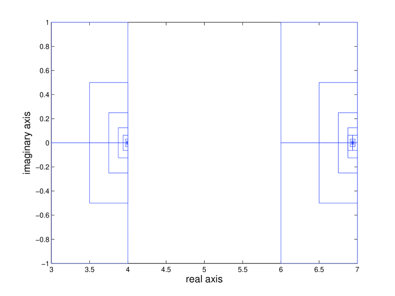
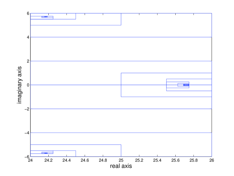
Figure 1: The regions explored by RIM for the disc with radius $1/2$, $n(x)=16$, and $\epsilon=1.0e-3$. Left: the search region is given by $S=[1,10]\times[-1,1]$. Right: the search region is given by $S=[22,25]\times[-8,8]$.

Example 2: Let $D$ be the unit square and $n(x)=16$ (AAS: I think this is correct) with $h\approx 0.05$. The matrices $A$ and $B$ are $2075\times 2075$. The exact transmission eigenvalues are not available. The first search region is given by $S=[3,8]\times[-1,1]$. RIM computes the following eigenvalues

$$\lambda_{1}=3.561,\quad\lambda_{2}=6.049,\quad\lambda_{3}=6.051.$$

They are consistent with the values given in Table 3 of [4]:

$$\lambda_{1}=3.479,\quad\lambda_{2}=5.883,\quad\lambda_{3}=5.891.$$

The second search region is given by $S=[20,25]\times[-8,8]$. The eigenvalues we obtain are

$$\lambda_{1}=20.574+5.128i,\quad\lambda_{2}=20.574-5.128i,\quad\lambda_{3}=21.595,\quad\lambda_{4}=23.412.$$

We plot the search regions in Fig. 2. The left picture is for $S=[3,7]\times[-1,1]$. The right picture is for $S=[20,25]\times[-6,8]$.

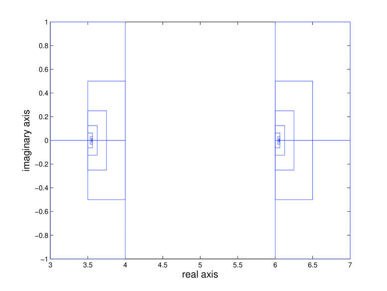
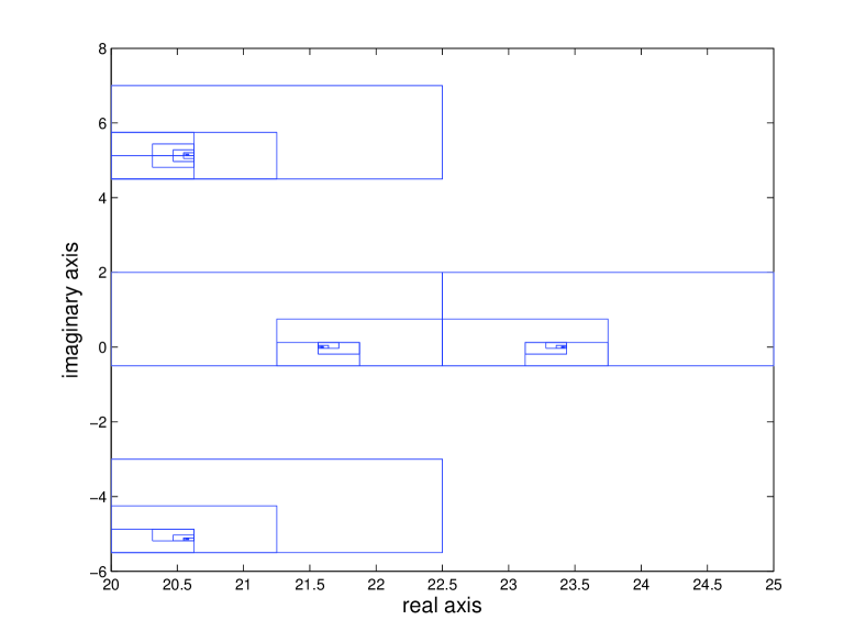
Figure 2: The regions explored by RIM for the unit square with $n(x)=16$ and $\epsilon=1.0e-3$. Left: the search region is given by $S=[3,7]\times[-1,1]$. Right: the search region is given by $[20,25]\times[-6,8]$.

5.2 Eigenvalues on $\Gamma:=\partial S$

It is very unlikely that $\Gamma:=\partial S$ is not contained in the resolvent set. However, we want to explore what will happen if eigenvalues lie on on $\Gamma$. The first example shows that this does not generate difficulty for RIM.

Example 3: We first consider a simple example given below (Example 5 of [23]):

$$A=\begin{pmatrix}\frac{99}{100}&\frac{1}{100}&0&\ldots&0\\ 0&\frac{98}{100}&0&\ldots&0\\ \ddots&\ddots&\ddots&\ddots&\vdots\\ 0&\ldots&0&\frac{1}{100}&\frac{1}{100}\\ 0&\ldots&\ldots&0&\frac{0}{100}\end{pmatrix},\quad B=\text{diag}(0,\ldots,0,1,\ldots,1),$$

where $B$ has $20$ ones on its diagonal. The following are some exact eigenvalues

$$\lambda_{1}=0,\quad\lambda_{2}=0.01,\quad\lambda_{3}=0.02,\quad\lambda_{4}=0.03.$$

We set the initial search region to be $S=[0,1/30]\times[0,1/100]$ and $\epsilon=1.0e-9$ and note that all the eigenvalues are on $\Gamma:=\partial S$.

The eigenvalues computed by RIM are given below (see also Fig. 3). They are accurate up to the required precision. From Fig. 3, we can see that RIM keeps refining around the eigenvalues.

$$\lambda_{1}=(4.967053731282552+4.967053731282552i)10^{-10},$$

$$\lambda_{2}=0.009999999900659+0.000000000496705i,$$

$$\lambda_{3}=0.020000000298023+0.000000000496705i,$$

$$\lambda_{4}=0.029999999701977+0.000000000496705i.$$

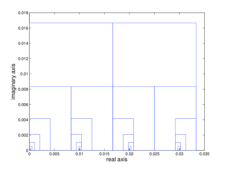
Figure 3: Eigenvalues on $\Gamma=\partial S$. All the four eigenvalues are on $\Gamma$.

5.3 Self-correction Property

When a quadrature point $z_{q}$ in the collection of linear systems (16) is close to an eigenvalue $\lambda$, the linear system will be ill-conditioned. In particular, when $\lambda$ is just outside $\Gamma$ the indicator function $\chi_{S}$ could be large because either the linear solve or quadrature rule are not sufficiently accurate. RIM will take such regions as admissible and refine. But fortunately, after a few subdivisions, RIM appears to discard the sub regions. We demonstrate this interesting self-correction property using two example.

Example 4: We use matrices $A$ and $B$ from Example 2 and focus on the eigenvalue located at $3.9945$. We choose the initial search region $S=[4.0,4.2]\times[0,0.2]$ and note that there is no eigenvalue in $S$. With the same standard two-point Gauss quadrature rule on each edge of $S$ RIM computes

$$\chi_{S}=4.383,$$ (17)

indicating that there may be eigenvalues in $S$ and RIM procedes to recursively explore $S$ by dividing $S$ into the four rectangles

$$S^{1}_{1}=[4.0,4.1]\times[-0.1,0],\quad S^{1}_{2}=[4.0,4.1]\times[0,0.1],$$

$$S^{1}_{3}=[4.1,4.2]\times[-0.1,0],\quad S^{1}_{4}=[4.1,4.2]\times[0,0.1]$$

with indicator values

$$\chi_{S^{1}_{1}}=1.589,\quad\chi_{S^{1}_{2}}=1.589,\quad\chi_{S^{1}_{3}}=0.002,\quad\chi_{S^{1}_{4}}=0.002.$$

RIM discards $S^{1}_{3}$ and $S^{1}_{4}$ and retains $S^{1}_{1}$ and $S^{1}_{2}$ as admissible regions.

We show the result for region $S^{1}_{1}$: $S^{1}_{2}$ is similar. The four rectangles from dividing $S_{1}^{1}$ are

$$S^{2}_{1}=[4.0,4.05]\times[-0.05,0],\quad S^{2}_{2}=[4.0,4.05]\times[-0.1,-0.05],$$

$$S^{2}_{3}=[4.05,4.1]\times[-0.05,0],\quad S^{2}_{4}=[4.0,4.05]\times[-0.1,-0.05],$$

with indicator values

$$\chi_{S^{2}_{1}}=0.997,\quad\chi_{S^{2}_{2}}=0.002,\quad\chi_{S^{2}_{3}}=0.002,\quad\chi_{S^{2}_{4}}=2.159e-04.$$

and RIM discards all the regions. Let us see one more level. Suppose $\chi_{S^{2}_{1}}$ is kept and subdivided into

$$S^{3}_{1}=[4.0,4.025]\times[-0.025,0],\quad S^{3}_{2}=[4.0,4.025]\times[-0.05,-0.025],$$

$$S^{3}_{3}=[4.025,4.05]\times[-0.025,0],\quad S^{3}_{4}=[4.025,4.05]\times[-0.05,-0.025]$$

with indicator values

$$\chi_{S^{3}_{1}}=0.395,\quad\chi_{S^{3}_{2}}=0.002,\quad\chi_{S^{3}_{3}}=0.001,\quad\chi_{S^{3}_{4}}=1.615e-04.$$

Hence RIM eventually discards $S$.

Example 5: The same experiment is conducted for a search region around the complex eigenvalue $\lambda=24.1586+5.690i$ with initial search region $S=[24.16,24.96]\times[5.30,6.10]$ which although close to the eigenvalue does not contain any eigenvalues. Indicator values are in Table. 1 and we can note that RIM does eventually conclude that there are no eigenvalues in the region.

Table 1: The indicators function $\chi_{S}$ on different search regions.

$S^{1}_{1}=[24.16,24.56]\times[5.30,5.70]$	11.825	$S^{1}_{2}=[24.16,24.56]\times[5.70,6.10]$	0.195
$S^{1}_{3}=[24.56,24.96]\times[5.30,5.70]$	5.418e-11	$S^{1}_{4}=[24.56,24.96]\times[5.70,6.10]$	4.119e-11
$S^{2}_{1}=[24.16,24.36]\times[5.30,5.50]$	9.216e-11	$S^{2}_{2}=[24.16,24.36]\times[5.50,5.70]$	3.682
$S^{2}_{3}=[24.36,24.56]\times[5.30,5.50]$	8.712e-14	$S^{2}_{4}=[24.36,24.56]\times[5.50,5.70]$	5.870e-11
$S^{3}_{1}=[24.16,24.26]\times[5.50,5.60]$	1.742e-11	$S^{3}_{2}=[24.16,24.26]\times[5.60,5.70]$	7.806
$S^{3}_{3}=[24.26,24.36]\times[5.50,5.60]$	1.476e-13	$S^{3}_{4}=[24.26,24.36]\times[5.60,5.70]$	6.755e-11
$S^{4}_{1}=[24.16,24.21]\times[5.60,5.65]$	6.558e-10	$S^{4}_{2}=[24.16,24.21]\times[5.65,5.70]$	2.799
$S^{4}_{3}=[24.21,24.26]\times[5.60,5.65]$	1.378e-13	$S^{4}_{4}=[24.21,24.26]\times[5.65,5.70]$	8.229e-11
$S^{5}_{1}=[24.16,24.185]\times[5.65,5.675]$	1.159e-8	$S^{5}_{2}=[24.16,24.185]\times[5.675,5.70]$	1.556
$S^{5}_{3}=[24.185,24.21]\times[5.65,5.675]$	4.000e-13	$S^{5}_{4}=[24.185,24.21]\times[5.675,5.70]$	8.648e-11
$S^{6}_{1}=[24.16,24.185]\times[5.65,5.675]$	5.574e-06	$S^{6}_{2}=[24.16,24.1725]\times[5.6875,5.70]$	0.095
$S^{6}_{3}=[24.185,24.21]\times[5.65,5.675]$	4.304e-12	$S^{6}_{4}=[24.185,24.21]\times[5.675,5.70]$	2.628e-11

5.4 Close Eigenvalues

RIM is able to separate nearby eigenvalues provided the tolerance is less than the eigenvalue separation.

Example 6: This example comes from a finite element discretization of the Neumann eigenvalue problem:

$$-\triangle u =\lambda u, \text{in }D,$$ (18a)

$$\frac{\partial u}{\partial\nu} =0, \text{on }\partial D,$$ (18b)

where $D$ is the unit square which has an eigenvalue $\pi^{2}$ of multiplicity $2$. We use linear Lagrange elements on a triangular mesh with $h\approx 0.025$ to discretize and obtain a generalized eigenvalue problem

$$A{\bf x}=\lambda B{\bf x},$$ (19)

where the stiffness matrix $A$ and mass matrix $B$ are $2075\times 2075$. The discretization has broken the symmetry and (19) the eigenvalue of multiplicity $2$ has been approximated by a very close pair of eigenvalues of

$$\lambda_{1}=9.872899741642826\quad\text{and}\quad\lambda_{2}=9.872783160389966.$$

With $\epsilon=1.0e-3$ ${\bf RIM}$ fails to separate the eigenvalues and we obtain only one eigenvalue

$$\lambda_{1}=9.872680664062500.$$

However, with $\epsilon=1.0e-9$ ${\bf RIM}$ separates the eigenvalues and we obtain

$$\lambda_{1}=9.872899741516449\quad\text{and}\quad\lambda_{2}=9.872783160419203.$$

The search regions explored by RIM with different tolerances are shown in Fig. 4.

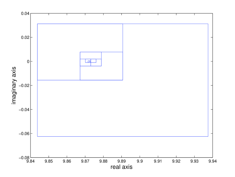
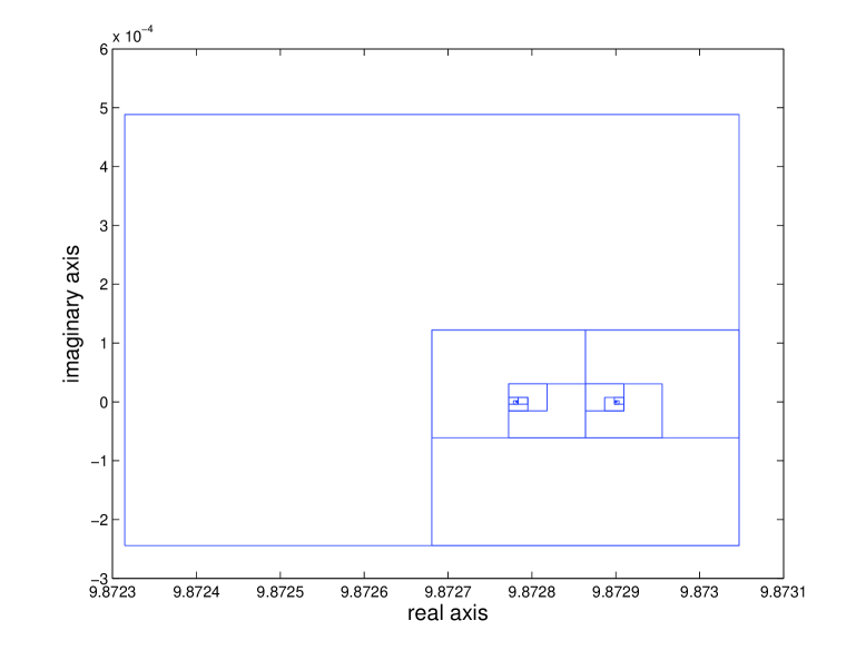
Figure 4: The regions explored by RIM. The search region is given by $S=[1,10]\times[-1,1]$. Left: $\epsilon=1.0e-3$. Right: $\epsilon=1.0e-9$.

Example 7: As a final example we compute the eigenvalues of the $40\times 40$ Wilkinson matrix

$$A=\begin{pmatrix}19&-1\\ -1&18&-1\\ \quad&\ddots&\ddots&\ddots\\ \quad&\quad&-1&1&-1\\ \quad&\quad&\quad&-1&1&-1\\ \quad&\quad&\quad&\quad&\ddots&\ddots&\ddots\\ \quad&\quad&\quad&\quad&\quad&-1&19&-1\\ \quad&\quad&\quad&\quad&\quad&\quad&-1&20\end{pmatrix}$$

which is known to have very close eigenvalues. With $\epsilon=1.0e-14$ and the search region $S=[-2,10]\times[-2,10]$. RIM accurately distinguishes the close eigenvalues with giving the results shown in Table 2 and Fig. 5.

Table 2: The computed Wilkinson eigenvalues by RIM.

$i$	$\lambda_{i}$	$i$	$\lambda_{i}$
1	-1.125441522046458	11	5.000236265619321
2	0.253805817279499	12	5.999991841327017
3	0.947534367500339	13	6.000008352188331
4	1.789321352320258	14	6.999999794929806
5	2.130209219467361	15	7.000000207904748
6	2.961058880959172	16	7.999999996191775
7	3.043099288071971	17	8.000000003841876
8	3.996047997334983	18	8.999999999945373
9	4.004353817323874	19	9.000000000054399
10	4.999774319815003	20	9.999999999999261

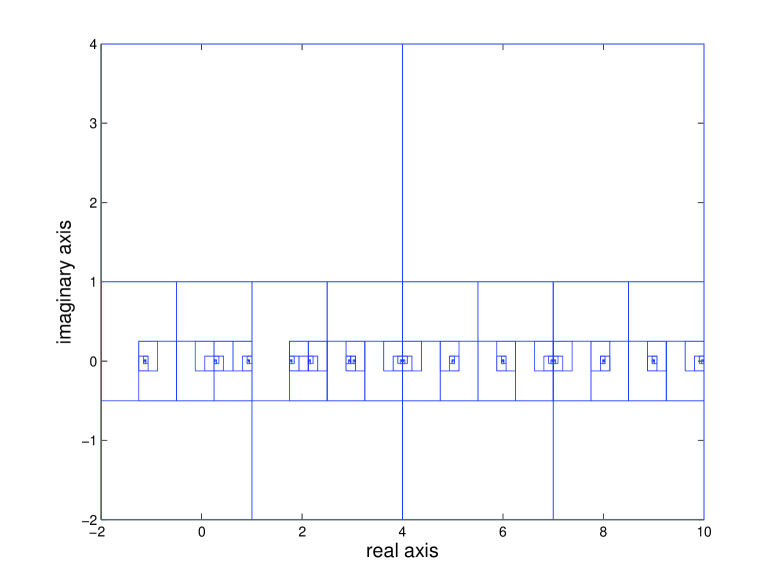
Figure 5: The regions explored by RIM for the Wilkinson matrix with $\epsilon=1.0e-14$.

6 Discussion and future work

This paper proposes a robust recursive integral method RIM to compute transmission eigenvalues. The method effectively locates all eigenvalues in a region when neither the location or number eigenvalues is known. The key difference between RIM and other counter integral based methods in the literature is that RIM essentially only tests if a region contains eigenvalues or not. As a result accuracy requirements on quadrature, linear solves, and the number of test vectors may be significantly reduced.

RIM is a non-classical eigenvalue solver which is well suited to problems that only require eigenvalues. In particular, the method snot only works for matrix eigenvalue problems resulting from suitable numerical approximations, e.g., finite element methods, of PDE-based eigenvalue problem, but also those eigenvalue problems which can not be easily casted as a matrix eigenvalue problem, e.g., see [3, 17].

The goal of this paper is to introduce the idea of RIM and demonstrate its potential to compute eigenvalues. A paper like this raises more questions than it answers. How inaccurate can the quadrature be and still locate eigenvalues? How inaccurate can the the linear solver can and still locate eigenvalues. The current implementation uses a combination of inaccurate quadrature and accurate solver: two point Gaussian quadrature on the edges of rectangles and the Matlab “$\backslash$” operator. These two separate issues can be combined into one question: how accurate does the overall procedure have to be to accurately distinguish admissible regions. These crucial complexity issues are not addressed in this current paper.

The example problems are small. We plan to extend RIM for large (sparse) eigenvalue problems which will require replacing “$\backslash$” with an iterative solver. Parallel extension is another interesting project since the algorithm is essentially embarrassingly parallel. In particular, a GPU implement of RIM is under consideration.

Acknowlegement

The work of JS and RZ is partially supported NSF DMS-1016092/1321391.

References

- [1] J. An and J. Shen, A Fourier-spectral-element method for transmission eigenvalue problems. Journal of Scientific Computing, 57 (2013), 670–688.
- [2] A.P. Austin, P. Kravanja and L.N. Trefethen, Numerical algorithms based on analytic function values at roots of unity. SIAM J. Numer. Anal. 52 (2014), no. 4, 1795-1821.
- [3] W.J. Beyn, An integral method for solving nonlinear eigenvalue problems. Linear Algebra Appl. 436 (2012), no. 10, 3839–3863.
- [4] F. Cakoni, D. Colton, P. Monk, and J. Sun, The inverse electromagnetic scattering problem for anisotropic media, Inverse Problems, 26 (2010), 074004.
- [5] F. Cakoni, D. Gintides, and H. Haddar, The existence of an infinite discrete set of transmission eigenvalues. SIAM J. Math. Anal., 42 (2010), 237–255.
- [6] F. Cakoni, P. Monk and J. Sun, Error analysis of the finite element approximation of transmission eigenvalues. Comput. Methods Appl. Math., Vol. 14 (2014), Iss. 4, 419–427.
- [7] D. Colton and R. Kress, Inverse Acoustic and Electromagnetic Scattering Theory, Springer-Verlag, New York, 3rd ed., 2013.
- [8] D. Colton, P. Monk and J. Sun, Analytical and Computational Methods for Transmission Eigenvalues. Inverse Problems Vol. 26 (2010) No. 4, 045011.
- [9] A. Cossonniére and H. Haddar, Surface integral formulation of the interior transmission problem. J. Integral Equations Appl. 25 (2013), no. 3, 341–376.
- [10] D. Gintides and N. Pallikarakis, A computational method for the inverse transmission eigenvalue problem. Inverse Problems 29 (2013), no. 10, 104010.
- [11] G. Hsiao, F. Liu, J. Sun and X. Li, A coupled BEM and FEM for the interior transmission problem in acoustics. J. of Comp. and Applied Math., Vol. 235 (2011), Iss. 17, 5213–5221.
- [12] S. Goedecker, Linear scaling electronic structure methods, Rev. Modern Phys., 71 (1999), 1085–1123.
- [13] X. Ji and J. Sun, A multi-level method for transmission eigenvalues of anisotropic media. Journal of Computational Physics, Vol. 255 (2013), 422–435.
- [14] X. Ji, J. Sun and T. Turner, A mixed finite element method for Helmholtz Transmission eigenvalues. ACM Transaction on Mathematical Softwares, Vol. 38 (2012), No.4, Algorithm 922.
- [15] X. Ji, J. Sun and H. Xie, A multigrid method for Helmholtz transmission eigenvalue problems. J. Sci. Comput., Vol. 60 (2014), Iss. 3, 276–294.
- [16] T. Kato, Perturbation Theory of Linear Operators, Springer-Verlag, 1966.
- [17] A. Kleefeld, A numerical method to compute interior transmission eigenvalues. Inverse Problems, 29 (2013), 104012.
- [18] A. Lechleiter, M. Rennoch. Inside-outside duality and the determination of electromagnetic interior transmission eigenvalues. SIAM Journal on Mathematical Analysis, 47(1) (2015), 684–670
- [19] T. Li, W. Huang, W.W. Lin and J. Liu, On Spectral Analysis and a Novel Algorithm for Transmission Eigenvalue Problems. Journal of Scientific Computing, Published online: 1 October 2014.
- [20] P. Monk and J. Sun, Finite element methods of Maxwell transmission eigenvalues. SIAM J. Sci. Comput. 34 (2012), B247–B264.
- [21] J. Osborn, Spectral approximation for compact operators. Math. Comp., 29 (1975), 712–725.
- [22] E. Polizzi, Density-matrix-based algorithms for solving eigenvalue problems. Phys. Rev. B, Vol. 79, 115112 (2009).
- [23] T. Sakurai and H. Sugiura, A projection method for generalized eigenvalue problems using numerical integration. Proceedings of the 6th Japan-China Joint Seminar on Numerical Mathematics (Tsukuba, 2002). J. Comput. Appl. Math. 159 (2003), no. 1, 119–128.
- [24] J. Sun, Estimation of transmission eigenvalues and the index of refraction from Cauchy data. Inverse Problems 27 (2011), 015009.
- [25] J. Sun, Iterative methods for transmission eigenvalues. SIAM Journal on Numerical Analysis, Vol. 49 (2011), No. 5, 1860 – 1874.
- [26] J. Sun, An eigenvalue method using multiple frequency data for inverse scattering problems. Inverse Problems, 28 (2012), 025012.
- [27] J. Sun and L. Xu, Computation of the Maxwell’s transmission eigenvalues and its application in inverse medium problems. Inverse Problems, 29 (2013), 104013.
- [28] X. Wu and W. Chen, Error estimates of the finite element method for interior transmission problems. Journal of Scientific Computing, 57 (2013), 331–348.