Complex Quantum Network Geometries:
Evolution and Phase Transitions
Abstract
Networks are topological and geometric structures used to describe systems as different as the Internet, the brain or the quantum structure of space-time. Here we define complex quantum network geometries, describing the underlying structure of growing simplicial 2-complexes, i.e. simplicial complexes formed by triangles. These networks are geometric networks with energies of the links that grow according to a non-equilibrium dynamics. The evolution in time of the geometric networks is a classical evolution describing a given path of a path integral defining the evolution of quantum network states. The quantum network states are characterized by quantum occupation numbers that can be mapped respectively to the nodes, links, and triangles incident to each link of the network. We call the geometric networks describing the evolution of quantum network states the quantum geometric networks. The quantum geometric networks have many properties common to complex networks including small-world property, high clustering coefficient, high modularity, scale-free degree distribution. Moreover they can be distinguished between the Fermi-Dirac Network and the Bose-Einstein Network obeying respectively the Fermi-Dirac and Bose-Einstein statistics. We show that these networks can undergo structural phase transitions where the geometrical properties of the networks change drastically. Finally we comment on the relation between Quantum Complex Network Geometries, spin networks and triangulations.
pacs:
89.75.Hc,89.75.Da,05.30.-dI Introduction
Networks are discrete structures that can be used to describe, model and understand a variety of real systems, including complex interacting systems RMP ; Newman_rev ; Boccaletti2006 ; Doro_book ; Santo or the microscopic nature of space-time spinnet1 ; spinnet2 ; Regge ; Rovelli .
Recently, in network science the characterization of the complexity of networks with geometrical and topological methods is gaining large momentum with several works related to the definition of curvature of the networks Yau1 ; Yau2 ; Jost ; Ollivier ; Keller1 ; Keller2 ; Higuchi ; Knill1 ; Saniee ; Gromov ; Mahoney_gromov ; Jonck ; Bary , persistent homology Vaccarino1 ; Vaccarino2 ; Mason , complex networks embedded in finite dimensions Doro_link ; det ; Apollonian ; Aste2 , and the study of the hyperbolicity of complex networks Kleinberg ; Aste ; Boguna_navigability ; Boguna_Internet ; Hyperbolic ; Boguna_growing ; Clough ; Reka ; Caldarelli .
In this context, it is becoming clear that in order to characterize the geometry of networks it is important to describe the underlying structure of simplicial complexes. A simplicial complex is constructed by gluing together simplices such as points, lines, triangles etc., along their faces. Therefore different works characterize ensembles of random simplicial complexes Farber1 ; Farber2 ; Kahle ; Krioukov_SC and their geometrical and topological properties. Recently a model for emergent complex network geometry has been proposed based on growing simplicial complexes SR .
In quantum gravity a central problem is to find the appropriate model describing the geometry of space-time at the quantum level. Different approaches have been proposed in which geometry emerges from some pregeometric phase Wheeler ; pregeometry_review ; pregeometry2 that include spin networks and loop quantum gravity spinnet1 ; spinnet2 ; Rovelli , spin foams Oriti , causal dynamical triangulations CDT1 ; CDT2 , causal sets Bombelli , energetic causal sets Smolin1 ; Smolin2 ; Smolin3 , network cosmology Cosmology , and quantum graphity graphity_rg ; graphity ; graphity_c . Network-like structures play a fundamental role in all these approaches.
This suggests that the emergence of geometric structure from the quantum description of networks is a more general mathematical problem that can be not only relevant for understanding the structure of space-time, but which might also help to understand general complex network structures.
Already in the early days of the field of network science the relation between complex network topologies and quantum statistics was shown in the framework of the Bianconi-Barabasi model Bose ; Fitness that is a growing network model with preferential attachment and fitness of the nodes which display a Bose-Einstein condensation. This model can also be extended to weighted networks Weighted described by the Bose-Einstein statistics and undergoing also the condensation of the weight of the links. The relation between growing Cayley trees with fitness of the nodes and Fermi-Dirac statistics has been found in Fermi and the underlying symmetries between the models in Bose and Fermi have been discussed in Complex . In the context of equilibrium network models it has been shown that quantum statistics emerges to describe simple or weighted networks Garlaschelli .
Here we characterize the non-equilibrium evolution of networks constructed from growing simplicial complexes of dimension two, i.e. formed by triangles, and such that to each link we associate an energy . We show that geometrical complex networks emerge from this dynamical evolution which display at the same time small-world network properties WS , exponential or scale-free degree distribution BA , high clustering coefficient and high modularity Santo . These networks can be either planar or non-planar with an Euler characteristic that is either (planar) or , where is the network size, indicating a finite average curvature in the network. As we will show in two limiting cases of this network dynamics, these networks describe the evolution of quantum network states. These network states are constructed along similar lines used in the quantum gravity literature graphity_rg ; graphity ; graphity_c by associating an Hilbert space to each node of the network and two Hilbert spaces to each possible link of the network. These network states evolve through a non equilibrium, Markovian dynamics. The network states can be mapped to geometric networks and have an evolution described by an appropriate path integral. The network dynamics describes the paths of single histories of networks on which the path integral is calculated.
We distinguish between Fermi-Dirac Networks and Bose-Einstein Networks. For both of them the number of triangles incident to a given link is . However, for Fermi-Dirac Networks can only take the values , whereas for Bose-Einstein Networks can take any integer value These networks evolve in such a way that at the global scale the average of over the links with energy follows the Fermi-Dirac statistics for the Fermi-Dirac Network and the Bose-Einstein statistics for the Bose-Einstein Network.
These network structures depend on an external parameter that we call the inverse temperature . As a function of they undergo major structural phase transitions in which the network structure changes drastically. In the case of the Fermi-Dirac Network, for the network is not any more small world, but acquires a finite Hausdorff dimensionality. In the case of the Bose-Einstein Network, for a link acquires a finite fraction of triangles, and the nodes at the end of the link acquire a finite fraction of all the links. This geometrical phenomenon is the Bose-Einstein condensation for these networks.
We observe here that the quantum network states studied in this paper are by no means the only way to associate a quantum state to a network. In particular in the quantum computation community, alternative approaches Mulken ; Huelga ; Perseguers ; Faccin ; Biamonte have been widely explored, characterizing quantum transport, quantum random networks, and quantum networks in which the links correspond to entangled states.
The paper is organized as follows. In Sec. II we describe the geometric network model with energy of the links depending on the parameter fixing the maximum number of triangles incident to a link. Moreover we define the entropy rate of the model and we describe the observed phase transition. In Sec. III we define the quantum network states. In Sec. IV. we define the evolution of the Fermi-Dirac quantum network state and the Bose-Einstein quantum network state. In Sec. V we study the Fermi-Dirac Network (given by the geometric network model with ). We show that this network characterizes the Fermi-Dirac quantum state, and we show that it is globally described by the Fermi-Dirac statistics. Finally we compare the analytical results to simulations and we describe the phase transition occurring at low temperatures. In Sec. VI we study the Bose-Einstein Network (given by the geometric network model with ) showing that it fully characterizes the Bose-Einstein quantum state, follows the Bose-Einstein statistics and undergoes the Bose-Einstein condensation at low temperatures. In Sec. VII we consider the thermodynamics of the networks and we consider the case in which we project the quantum network state on an unlabeled final network state. In Sec. VIII we generalize the geometric model introducing a new parameter and a new process of addition of triangles that allows for the generation of network geometries that are not planar. We characterize the geometry of these networks and we describe the phase transitions observed at low temperature. In Sec. IX we generalize the evolution of the quantum network states corresponding to the generalized geometric network model. In Sec. X we describe the dual of the networks generated by the proposed model and we comment on the relation between the Fermi-Dirac Network and spin networks. In Sec. XI we comment on the relation between Complex Quantum Network Geometries, triangulations and foams. Finally in Sec. XII we give the conclusions.
II Geometric network with energy of the links
II.1 Evolution of the geometric networks with energy of the links
Real networks display at the same time several structural properties (including finite clustering coefficient, significant modularity, finite spectral dimension, heterogeneous degree distribution) that have been shown to be captured by a very simple model of emergent geometry recently introduced by the authors SR . The model proposed in SR is a non-equilibrium model of growing simplicial complexes of dimension , i.e. formed by gluing triangles along their edges. In this model each link can belong at most to a number of triangles where the parameter can take any finite value or the value , indicating the case in which each link can belong to an arbitrarily large number of triangles. In the case the model reproduces random manifolds of dimension with an exponential degree distribution and random distribution of local curvatures, in the case the model generates scale-free networks with finite clustering coefficient and significant modularity quantifying the relevance of their community structure.
In SR all the nodes and all the links are treated equally, having the same probability to attract new triangles. Nevertheless, in complex systems, attaching a new triangle to a given link might not have the same probability of attaching it to another link.
Already in the context of complex networks growing by preferential attachment RMP ; Newman_rev , the heterogeneity of the nodes in attracting new links has been recognized to be essential to characterize the evolution of networks, as for example the World-Wide-Web or the Internet Fitness ; Bose . Usually, this heterogeneous ”quality” of the nodes is modeled by associating each node to an energy drawn from a given distribution. Interestingly, complex networks with energy of the nodes have been shown Bose ; Fermi to be characterized by quantum Bose-Einstein and Fermi-Dirac statistics, and might display a Bose-Einstein condensation in which one node grabs a finite fraction of the links. This phase transition is relevant for a number of complex networks including economical, technological and social networks in which nodes connected to a finite fraction of the nodes might emerge.
In the quantum gravity literature, the relation between networks and quantum states has been recently explored graphity_rg ; graphity ; graphity_c to construct models of emergent space-time geometry. In these works, each network is associated to a quantum network state and the network structure is dictated by an equilibrium Hamiltonian dynamics.
Here we consider networks constructed by a non-equilibrium dynamics describing the underlying structure of simplicial complexes constructed by the addition of connected complexes of dimension , i.e. triangles. These networks display non trivial geometrical properties, characterizing in some limit planar random manifolds, as will be discussed later in the paper. For this reason we call them geometric networks. As in the geometric network model SR we assume that each link can belong at most to a number of triangles. Moreover we associate energies both to nodes and links describing the different ability of nodes and links to attract new triangles.
In studying this model our goal is two-fold. On one side we aim at characterizing a wider class of emergent geometries, and their possible structural phase transitions in order to unveil the basic geometric properties of complex networks. On the other side we aim at furthering our understanding on the relation between the network evolution and quantum mechanics by exploring the connection between network evolution, quantum statistics, and evolution of quantum network states constructed using methods similar to the one introduced in graphity_rg ; graphity ; graphity_c .
The energies of the nodes and of the links are defined as follows. Every node of the network is associated with the energy of the link drawn from a distribution note . The energy is assigned to the node when the node is added to the network and is quenched during the growth of the network. Every link between node and node is associated with the energy of the link which is a given symmetric function of the energy of the two nodes and , i.e.
| (1) |
with .
We define the so called spin of the link as
| (2) |
The spins of the links belonging to a triangle between the nodes , and satisfy the conditions
| (3) |
This result remains valid for any permutation of the order of the nodes and belonging to the triangle. Although most of the derivations shown in this paper can be performed similarly for either continuous or discrete energy of the nodes and of the links, here we consider the case in which the energies of the nodes and the energy of the links are discrete. In particular, if the energy of the nodes takes integer values, the spin of the links takes half-integer values and Eqs. can be interpreted as the Clebsch-Gordon relations between the half-integer spins of the links of each triangle. This property motivates dubbing this variable a spin.
Specific expressions of the energy of the link might depend on the spin of the link. Examples of specific choices for the energy of the link are the quadratic relation,
| (4) |
or the linear relation
| (5) |
Here we want to keep the generality of the model and we will take given by Eq. unless a specific functional form of the energy of the link is indicated.
The geometric network model is the underlying network of a simplicial complex of dimension formed by gluing triangles along the edges. We assume that each link can belong at most to a number of triangles where the parameter can take any finite value or the value , indicating the case in which each link can belong to an arbitrarily large number of triangles. We call the links to which we can still add at least one triangle unsaturated. All the other links we call saturated. In the case , all the links are unsaturated. We start at time from a network formed by a single triangle, a simplex of dimension . At each time we add a triangle to an unsaturated link of the network. We choose this link with probability given by
| (6) |
where is given by
| (7) |
Here we introduced several time-dependent quantities which we will use repeatedly in this paper: is the element of the adjacency matrix of the network, is equal to one (i.e. ) if the number of triangles to which the link belongs is less than , otherwise it is zero (i.e. ), is equal to the total number of triangles incident to the link . Having chosen the link the simplicial complex at time is constructed by adding a node , two links and and the new triangle linking node , node and node . The geometric complex network is the network structure of the resulting simplicial complex.
Therefore the number of nodes of the network grows linearly with time and is given by .
The linking probability depends on the parameter that we call inverse temperature. For , all the links that are unsaturated have equal probability to be selected. For instead, unsaturated links with low energy are more likely to be selected than links with higher energy.
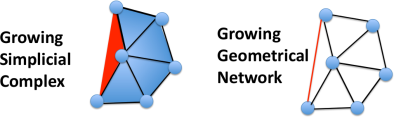
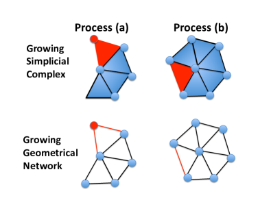
With the above algorithm we describe a growing simplicial complex formed by adding triangles. From this structure we can extract the corresponding network where we consider only the information about node connectivity (which node is linked to which other node). We call this network model the geometrical growing network. In Figure 1 we show schematically the dynamical rules for building the growing simplicial complexes and the growing geometrical networks that describe its underlying network structure. In the following we will focus in particular on the limiting cases in which (-dimensional manifolds), or . For reasons that will become clear in the following, we will call the growing geometric network with the Fermi-Dirac Network and the one with the Bose-Einstein Network. In Figure 2 we show examples of the first few steps of their evolution. The Fermi-Dirac Network and the Bose-Einstein Network will also be indicated as quantum geometric networks.
II.2 Entropy rate of the network evolution
Entropy measures for network evolution are very important characteristics for evaluating the interplay between randomness and order in these structures Entropyrate ; VonNeumann ; Garnerone ; Hancock . In particular, for growing network models, the entropy rate Entropyrate characterizes how the space of typical network dynamical evolutions increases with time. A change in the scaling of the entropy rate typically indicates a phase transition in the network Entropyrate . The geometric network evolution is described by the sequence where indicates the energy of the node added to the network at time , indicates the link chosen at time with probability given by Eq. (6). At any given time, therefore, indicates the link to which the new triangle is attached.
The entropy rate of the network evolution can be expressed as
| (8) | |||||
where is the probability that, given the temporal evolution of the network until time , at time a new triangle is attached to the link with the new node of this triangle having energy .
At time the probability that the new node has energy is given by the probability distribution , and it is independent of the previous evolution of the network. The probability of choosing the link is given by that depends on the previous history of the network. Moreover and are independent. Therefore the entropy rate can be written as
| (9) |
with , specified below. In particular is the contribution to the entropy rate due to the random distribution of the energy of the nodes, it is independent of time and is given by
| (10) |
The quantity of the growing geometric network evolution defines the contribution to the entropy rate due to the choice of the link where the new triangle is attached and is given by
| (11) |
evaluated at time . With Eq. , we get
| (12) |
where
| (13) |
We note here that, as the inverse temperature changes, we might expect a phase transition in the network characterized by a different scaling of the entropy rate and the normalization constant with time below and above the transition.
The normalization constant is fixed by Eq. . For , grows linearly with time . In fact for and , only if and only if . Moreover, since at each time we add two unsaturated links and we remove one unsaturated link,
| (14) |
For and instead, all the links are unsaturated, i.e. and every triangle is incident to three links. Therefore, since we add a triangle for every time step,
| (15) |
For a significant range of values of we will still continue to have for because is a sum over a linearly growing set of non-zero variables. For however, only the unsaturated links with minimal energy of the links will contribute to the sum defined in Eq. because the dynamics becomes extremal. Therefore we can have . In this case a phase transition is expected to occur in the network at the structural level. This phase transition induces a substantial change in the geometry of the networks above and below the transition as discussed in the next paragraph.
II.3 Phase transition in geometric networks
The networks constructed according to the model defined in Sec. II.1 are planar. In fact the Euler number of the simplicial complex from which they are extracted is constant during the network evolution and is given by
| (16) |
where is the total number of nodes, is the total number of links and is the total number of triangles.
Let us prove this result recursively. At time the geometrical networks are formed by a single triangle . Therefore we have
| (17) |
At each time step we add a single node, two links and one triangle, therefore
| (18) |
This shows that the simplicial complexes constructed by gluing new triangles to a single existing link of the network have Euler characteristic . When considering the network underlying each of these simplicial complexes, and embedding it in a plane, one can see that the number of faces of the embedded graph is in fact equal to the number of triangles of the simplicial complex when we do not count the external face of the planar network. Therefore these networks are planar.
Another, equivalent way to prove that our networks are planar is to observe that these networks, by construction, do not contain any complete graphs of five nodes (subgraph ) or any bipartite complete graph of six nodes (subgraph ).
Additionally we define the boundary of the network, as the set of unsaturated nodes and links. Unsaturated links, are links with , while unsaturated nodes are nodes with at least an incident unsaturated link. Note that in the geometric networks studied here, all the nodes are unsaturated since by construction they are always incident to exactly two unsaturated links. Therefore all the nodes of the network belong to its boundary. For these networks the curvature Keller1 ; Keller2 associated to each node is given by
| (19) |
where indicates the degree of node , indicates the total number of triangles incident to node , and where the last equation can be derived by considering that in the present model for every . The last expression in Eq. , relating the curvature of node to the number of triangles incident to it, has an intuitive explanation. As all triangles are isosceles, and each node is at the boundary of the network,each node incident to exactly triangles will have zero curvature, since the sum of the angles incident to it is .
Here we focus on the quantum geometric networks (cases and ) and we study the geometry of these network models as a function of . These networks are generated by a non-equilibrium dynamics that does not contain any indication about any embedding space. In the case , the Fermi-Dirac Neworks are planar manifolds describing random geometries, In the case , the Bose-Einstein Networks are planar scale-free networks but are not manifolds.
Here we show numerical evidence that for given distribution and energy of the links a structural phase transition can occur in quantum geometric networks. Specifically, we consider the case in which can only take integer values and the distribution is Poisson with average , i.e.
| (20) |
Moreover we take the energy of the generic link given by Eq. (5).
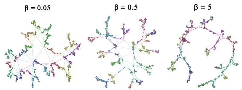
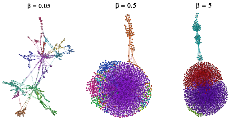
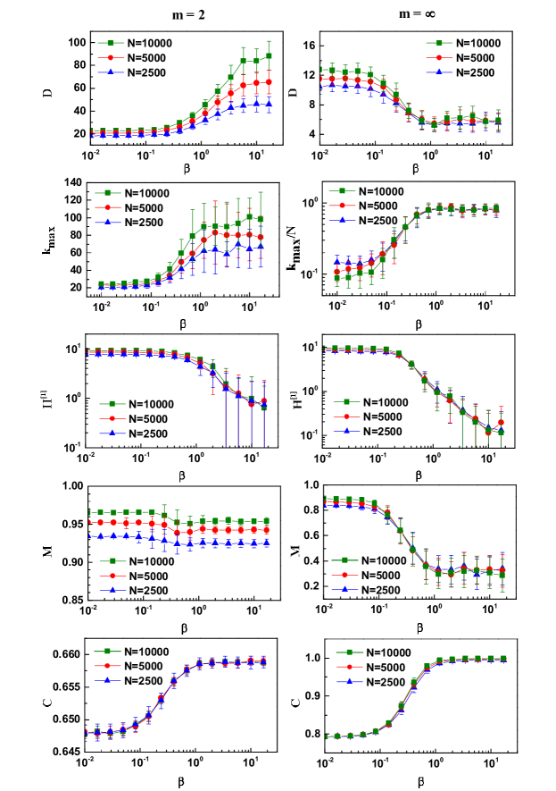
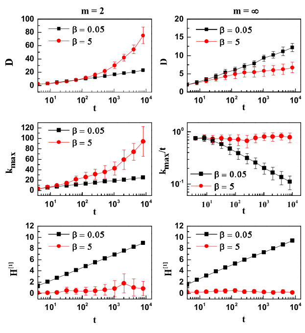
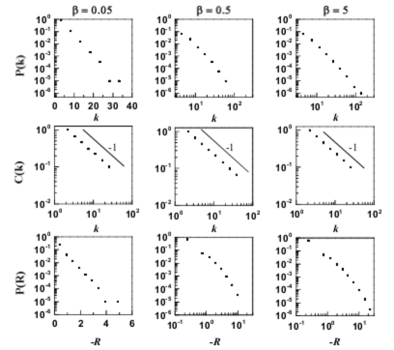
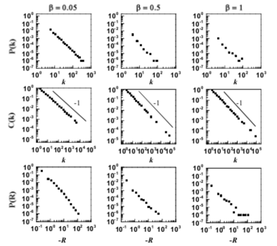
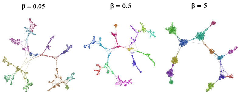
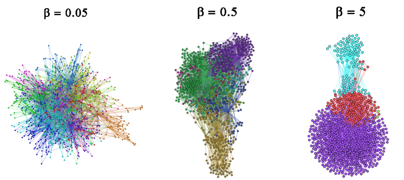
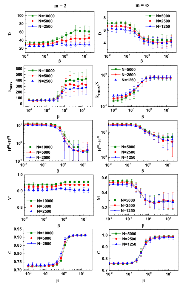
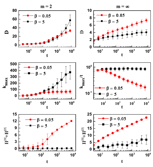
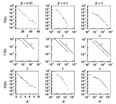
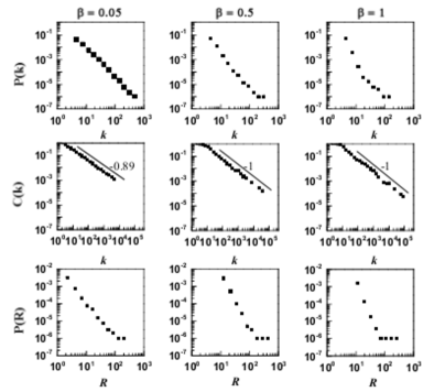
As a function of we observe a phase transition in both the Fermi-Dirac Network and the Bose-Einstein Network. For the structure of the network and its geometry change drastically as can already be seen from the visualizations of the networks (Figure 3 for the Fermi-Dirac Network and Figure 4 for the Bose-Einstein Network). The transition is characterized by a different scaling of the entropy rate below and above . For increases with time as , due to the linear scaling of , while, for , and fluctuates widely during the network evolution. Here we discuss in detail the consequences of this transition in the Fermi-Dirac Network and in the Bose-Einstein Network. In Figure 5 we show major geometrical and structural properties of the network as a function of the inverse temperature across the phase transitions. In particular we display the maximal shortest (hopping) distance from a given node of the initial triangle , the maximal degree of the network, the entropy rate , the modularity Newman calculated using the Louvain algorithm Louvain and the average clustering coefficient across the phase transitions. In Figure 6 we show major geometrical and structural properties of the network as a function of time for given values of the inverse temperature below and above the phase transition. Finally in Figure 7 and Figure 8 we show the degree distribution , the average clustering coefficient of nodes of degree , and the distribution of the curvature , for the Fermi-Dirac and the Bose-Einstein Network above and below the phase transition.
For the Fermi-Dirac Network, the most important indicator of the phase transition is which grows logarithmically with time for , and as a power-law for . Therefore the network is small-world for while it has finite Hausdorff dimension for . Moreover the maximum degree increases significantly below the transition for .
Furthermore, for , the degree distribution is exponential, and the distribution of the curvature
has a negative exponential tail,the average curvature is and its second moment is finite.
For , instead, follows a power-law, and
has a negative power-law tail. In this case, the average
curvature is , but its second moment diverges. For every value of , the network has high modularity and a hierarchical structure Ravasz
with an average clustering coefficient of nodes of degree decaying as and .
For the Bose-Einstein Network, the most important indicator of the phase transition is the maximum degree which scales sub-linearly with time for and linearly for , i.e. in this case the most connected node is linked to a finite fraction of all the nodes. Moreover, for , increases logarithmically with the network size, i.e. the network is small-world, while for it decreases significantly.
Furthermore, for , the degree distribution is scale-free,
the network has high modularity ,
and the distribution of the curvature has a negative power-law tail.
For , instead,
is dominated by outlier hubs,
the network has low modularity
and has a negative tail dominated by outlier nodes.
In both cases, the average curvature is , and its second moment diverges.
The network has a hierarchical structure Ravasz with an average clustering coefficient of nodes of degree decaying as and .
III Quantum network states
III.1 The Hilbert space
Using a similar approach used already in graphity_rg ; graphity ; graphity_c , here we define quantum network states. In graphity_rg ; graphity ; graphity_c an Hilbert space is associated to each node and each possible link of a network of nodes. Here we associate to each node and Hilbert space and to each link we associate two Hilbert spaces and . The total Hilbert space of a network of nodes is given by
| (21) |
A single realization of a growing geometric network of size in which the nodes are labelled by the time they have been added to the network can be mapped to a quantum state by mapping the nodes, the links and the triangles of the network to quantum states as described in the following.
III.2 Nodes quantum states
To every node we associate a Hilbert space which the Hilbert space of a fermionic oscillator with energy . Therefore, to every node of the network we associate a node quantum state that can be decomposed in the basis
| (22) |
with . The state
| (23) |
is said to contain a particle of energy and can be mapped to the presence of the node with energy in the network. The state
| (24) |
is an empty state and can be mapped to the absence of the node in the network. In this case the value of is irrelevant to characterize the state.
III.3 Link quantum states
To every possible link of a network we associate an Hilbert space .The Hilbert space is chosen to be that of a fermonic oscillator. To every pair of nodes in the network we associate a link quantum state that can be decomposed in the basis
| (25) |
where . The state
| (26) |
is said to contain a particle and is mapped to a link in the network. The state
| (27) |
is an empty state and is mapped to the absence of a link in the network.
III.4 Incident triangles quantum state
To every possible link of a network we associate an Hilbert space . For the Fermi-Dirac network state we will assume that this Hilbert space is the one associated to a fermionic oscillator. For the Bose-Einstein network state we will assume that this Hilbert space is instead associated with a bosonic oscillator. Therefore to each possible link of the network we associate a incident triangles quantum state that can be decomposed in the basis
| (28) |
with for the Fermi-Dirac Network and for the Bose-Einstein Network. The quantum number of links for which , is mapped to the number of triangles exceeding one incident to every existing link . Therefore if we can only have while if we can have any integer value of the occupation number .
III.5 Quantum network states
At each time the quantum network state can be decomposed into a basis
| (29) |
We consider the following operators that act on the nodes, links and incident triangles quantum states.
III.6 Creation-Annihilation operators
The operators are creation-annihilation of node quantum states and have anti-commutation relations
| (30) |
where is the Kronecker delta, for and otherwise. They act on the node states as
| (31) |
The operators are creation-annihilation operator of link quantum states and have anti-commutation relations
| (32) |
where if and or if and and otherwise. They act on the link states as
| (33) |
Finally we define two classes of creation annihilation operators acting respectively on the incident triangles quantum states of Fermi-Dirac and Bose Einstein quantum network states. The creating and annihilation operators and acting on incident triangle quantum states of Fermi-Dirac network states are anti-commuting,i.e.
| (34) |
When these operators act on the incident triangles quantum states, they can only generate occupation numbers . Their action on the basis is given by
| (35) |
The creation annihilation operators and that are acting on the incident triangles quantum states of the Bose-Einstein quantum network states have the commutation relations
| (36) |
When these operators act on the incident triangles quantum states, they can generate arbitrary occupation numbers Their action on the basis is given by
IV Evolution of quantum network states
In this section we define a non equilibrium Markovian evolution of the quantum network states. The possibility of a Markovian evolution of quantum network states is not entirely new in the literature, as it has been for example proposed in graphity_rg . Therefore we will define a quantum network state and its evolution with time. The quantum network state at every time step can be decomposed into the base
We start from an initial condition at given by
where is fixed by the normalization condition . The quantum evolution of the network state is given by a Markov process whose transition rate is determined by the unitary operator
| (38) |
where is defined by
| (39) | |||||
Here as in Eq. (1) and is fixed by the normalization condition . The quantum operators , can take two different values, defining in this way the Fermi-Dirac Quantum Network state and the Bose-Einstein Quantum Network state, i.e.
| (41) |
In the following section we will consider in detail the Fermi-Dirac and the Bose-Einstein Quantum Network states.
V Fermi-Dirac Quantum Network Evolution
V.1 Path integral
The evolution of the Fermi-Dirac Quantum Network state is given by
| (42) |
where and is fixed by the normalization condition .
Using the definitions of the creation and annihilation operators defined in Sec. III, the normalization constant of the Fermi-Dirac Quantum Network state is fixed by the path integral
| (43) |
for . Here is a sequence of links and is a sequence of energies of the nodes that describes a single history over which the path integral is calculated. In the path integral in Eq. each path is assigned a weight
| (44) | |||||
where the terms and that appear in Eq. can be expressed in terms of the history as
| (45) |
Therefore can be interpreted as a partition function of a statistical mechanics problem in which each path up to time has probability
| (46) |
Each of the paths can be mapped to a geometrical network evolution with . In this mapping indicates the energy of the node added to the network at time , indicates the link to which we attach a new triangle at time , indicates the adjacency matrix of the network, indicates the additional number of triangles incident to an existing link . The probability of each geometrical network evolution described in Sec. II.1 is the same as the weight that the corresponding history has in Eq. .
Starting from Eq. we can calculate the conditional probability that at time we add a link given the present state of the network evolution, . A straightforward calculation shows that
| (47) |
where
| (48) |
Given that has the graphical network interpretation , i.e. indicates that the link is not saturated, while indicates that the link is saturated, i.e. , the expression in Eq. is the same as defined in Eq. . It follows that studying the geometrical network evolution for determines the properties of the Fermi-Dirac quantum network state. For this reason we call the growing geometrical network with the Fermi-Dirac Network.
V.2 Fermi-Dirac Statistics
The average of the quantum number over all the links of the Fermi-Dirac Network follows the Fermi-Dirac distribution. Since , equivalently, we can say that the probability that a link with energy is saturated follows the Fermi-Dirac statistics. To derive this result, let us consider the master equation Doro_book for the number of links (with , and ), that have at time . Since at each time we choose a link with probability , only if it is unsaturated (i.e. ), we add one triangle to the link (i.e. ) and we add other two unsaturated links, the master equation reads
| (49) | |||||
where and is the probability that a new link of the network with links two nodes with energy and . In order to solve this master equation we assume that the normalization constant and we put
| (50) |
This is a self-consistent assumption that must be verified by the solution of Eqs. . Moreover we also assume that at large times . In fact the number of links in the network is for . Here indicates the asymptotic probability that a random link with and , has . With these assumptions, we can solve Eqs. finding
| (51) | |||||
where and is the Fermi-Dirac occupation number
| (52) |
Considering all the links with energy , we have
| (53) |
where
| (54) |
and where
| (55) |
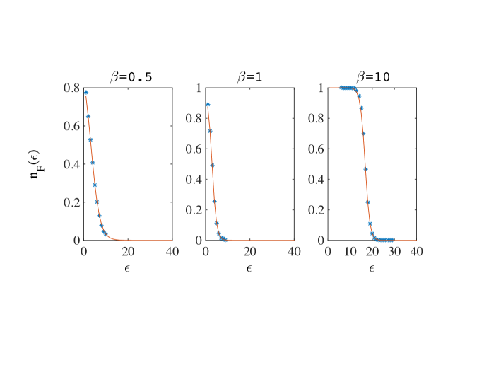
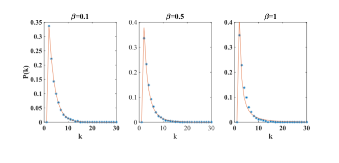
Therefore, in the Fermi-Dirac Network the average of the incident triangles quantum number over links of energy follows the Fermi-Dirac distribution.
To complete the solution it is necessary to find the correct expression for . Since by definition is the energy of the new node attached to the network at time , and since this energy is drawn randomly from a distribution , we have that the probability can be factorized,
| (56) |
where is the probability that a new triangle is attached to a link having at its end a node of energy and is thus normalized. Therefore we can write a recursive equation for . Since we attach new triangles to random unsaturated links with energy with probability , it follows that the recursive equation for reads
| (57) | |||||
where in the last equation we have used the expression for given by Eq. (51). Eq. can be formulated as the eigenvalue problem
| (58) |
where
| (59) | |||||
Since we require that is a probability, i.e. it is non-negative and normalized, the solution of the eigenvalue problem is given by the Perron-Frobenious eigenvector of the matrix satisfying
| (60) |
Finally the chemical potential is fixed by the self-consistent condition in Eq. that can be rewritten as
| (61) |
which is the same equation as the one fixing the chemical potential in a Fermi gas Kardar with density of states , inverse temperature and specific volume . If the self-consistent equation given by Eq. has a solution, and , the master equation asymptotically in time has a stationary solution given by Eqs. (51). This implies that the average of the quantum numbers over links of energy , i.e. , follows the Fermi-Dirac distribution.
V.3 Structural properties of the Fermi-Dirac model
Let us here characterize some of the important structural properties of the Fermi-Dirac network model. First of all, let us consider the degree distribution . In order to find we first write the master equation for the number of nodes that at time have degree given that they have energy . For simplicity in this paragraph we consider the linear relation Eq. (5) between link and node energies.
The master equation Doro_book for reads
| (62) | |||||
where we have assumed that asymptotically in time we can define the chemical potential given by
By assuming in the large network limit that , solving Eq. (62) we get,
| (63) |
for . Therefore, summing over all the values of the energy of the nodes we get the full degree distribution
| (64) |
for .
The curvature of a node is given by
| (65) |
So the distribution of the curvature is given by
| (66) |
where . Therefore the distribution of the curvature is decaying exponentially for negative values of the curvature.Moreover the average curvature is and the fluctuations around this average are bounded,i.e. .
V.4 Comparison with numerical simulations
Here we numerically simulate a Fermi-Dirac Network Evolution in which the energies of the nodes are non-negative integers with given by a Poisson distribution with average as in Eq. (20) and link and node energies related linearly Eq. (5).
We compare the results of the theory with the outcomes of the simulations as long as the chemical potential defined in Eq. is well defined. In particular we show the results of simulations confirming that the average of the quantum number over the links of energy , is given by Eq. and follows the Fermi-Dirac statistics. In Figure 9 we compare the results of the simulations with the theoretical expectations by plotting the right and left hand side of equation
| (67) |
equivalent to Eq. and the degree distribution of this network with the theoretical expectation given by Eq. (64). We find very good agreement in both cases as displayed in Figure 10.
V.5 Phase transition in the Fermi-Dirac network
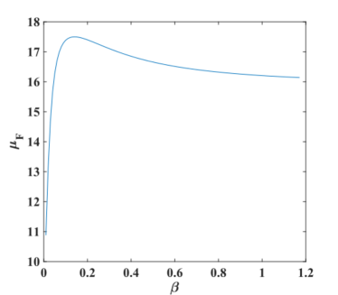
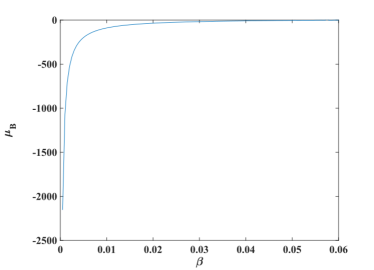
The self-consistent approach for solving the Fermi-Dirac network is based on the assumption that the chemical potential of the network defined in Eq. exists. But in the network it is possible to find a phase transition at high enough inverse temperature, i.e. for where this assumption fails (see Sec. II.3). In order to determine where this phase transition occurs we have solved the self-consistent equation for the chemical potential given by Eq. . This equation can always be solved to find the chemical potential , but the value of the chemical potential as a function of the inverse temperature can have a maximum for . Here we have identified this maximum with the onset of the phase transition. In fact, from the dynamic rules of the model it is clear that the network dynamics for increasing value of tends to attach new triangles on unsaturated nodes with lower energy. Therefore if the probability is given by Eq. the chemical potential that can only increase with increasing inverse temperature .
In Figure 11 we show the chemical potential as a function of the inverse temperature for a Fermi-Dirac network with a Poisson distribution (given by ) with average and linear relation between the energy of the nodes and the energy of the links (Eq. ). In order to perform the numerical calculation of the chemical potential the distribution is truncated at a cutoff value . The chemical potential has a maximum at which is a good prediction for the phase transition as can be seen from the simulation results shown in Figure 5.
VI Bose-Einstein Network Evolution
VI.1 Path integral
The evolution of the Bose-Einstein quantum state is described by the unitary operator defined in the following,
| (68) |
where and is fixed by the normalization condition .
In this case the normalization constant is given by the path integral
| (69) |
for and . Here is a sequence of links and a sequence of energies of the new nodes that describes a single history over which the path integral is calculated. Each path in Eq. is assigned a weight
| (70) | |||||
where and can be expressed in terms of the history in the same way as in Eq. (V.1). Note the characteristic sign difference in Eq. (70) compared to the Fermi-Dirac case. Therefore can be interpreted as a partition function of a statistical mechanics problem in which each path up to time has probability
| (71) |
Each of the paths can be mapped to a geometrical network evolution with . In this mapping indicates the energy of the node added to the network at time , indicates the link to which we attach a new triangle at time , and indicates the adjacency matrix of the network. Moreover indicates the number of triangles that exceed one, attached to the link . The probability of each geometrical network evolution described in Sec. II.1 is the same as the probability given by in Eq. .
Starting from Eq. we can calculate the conditional probability that at time we add a link given the present state of the network evolution, . A straightforward calculation shows that
| (72) |
where
| (73) |
The expression in Eq. is the same as defined in Eq. for . In this case for nodes for which there is a link, i.e. . It follows that studying the geometrical network evolution for determines the properties of the Bose-Einstein quantum network state. For this reason we call the growing geometrical network with the Bose-Einstein Network.
VI.2 Bose-Einstein statistics
In the Bose-Einstein Network the average of the quantum number over links with energy follows the Bose-Einstein distribution. To show this result let us consider the master equation Doro_book for the number of links (with and and ) that have at time . Since at each time we choose a link with probability , the master equation reads
where and is the probability that a new link will connect a new node with energy and an old node with energy . In order to solve this master equation we assume that the normalization constant and we put
| (75) |
Moreover we also assume that at large times as the number of links in the network is for . The quantity indicates the asymptotic probability that a random link with and and , has . Making these assumptions, it is possible to solve Eq. getting
| (76) | |||||
for . Eq. is automatically normalized once the distribution is normalized. Therefore the average of the quantum numbers over links with energy is given by
| (77) | |||||
where indicates the Bose-Einstein occupation number
| (78) |
Summing over all the links with energy , we get
| (79) |
where
| (80) |
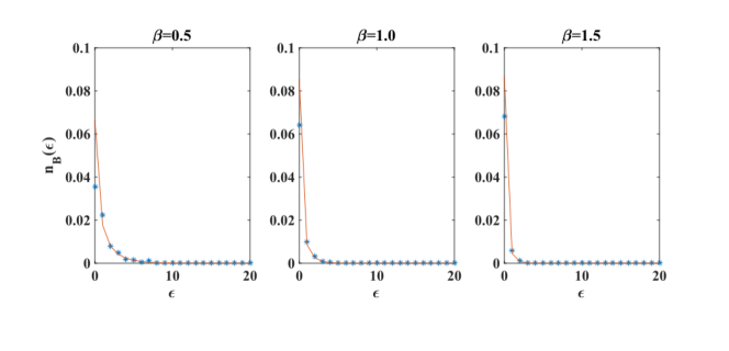
Therefore in the Bose-Einstein network the average of the quantum number over links of energy follows the Bose-Einstein distribution.
To complete the solution it is necessary to find the correct expression for . Since by definition is the energy of the new node attached to the network at time , and since this energy is drawn randomly from a distribution , the probability can be factorized,
| (81) |
where is the probability that a new triangle is attached to a link having at its end a node of energy and is therefore normalized.
We can write a recursive equation for . In fact we have
| (82) | |||||
where in the last equation we have substituted Eq. into . This equation can be formulated as the eigenvalue problem
| (83) |
where
| (84) | |||||
Since we require that is a probability, i.e. it is non-negative and normalized, the solution of the eigenvalue problem is given by the Perron-Frobenious eigenvector of the matrix satisfying
| (85) |
By imposing the self-consistent condition in Eq. we find the equation determining the chemical potential ,
| (86) |
which is the same equation as the one fixing the chemical potential in a Bose gas Kardar with density of states , inverse temperature and specific volume .
If the self-consistent Eq. has a solution, this implies that the average of the quantum number over links of energy , , follows the Bose-Einstein distribution.
VI.3 Structural properties of the Bose-Einstein Network
In this section we derive the degree distribution and the distribution of the curvature in the case in which the energies of the links are linearly dependent on the energies of the nodes as in Eq. (5). In order to derive the degree distribution in this case, let us write the master equation Doro_book for the number of nodes that at time have degree and energy , i.e.
| (87) | |||||
where we have assumed self-consistently that asymptotically in time is defined as
| (88) |
Assuming that asymptotically in time we find the expression for and substituting this expression in Eq. we have,
| (89) |
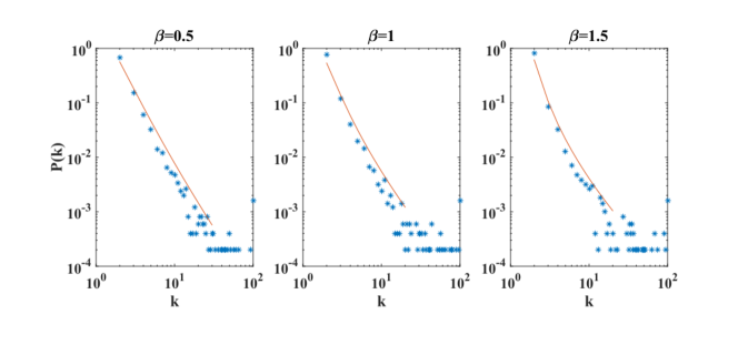
for . Therefore the degree distribution of the entire network is scale-free and given by
for . The fraction of the total number of links attached to nodes with energy is given, asymptotically in time, by
| (91) |
where is defined as
| (92) |
In Eq. the first term indicates the fraction of links initially attached to the new nodes of energy , and is therefore given by because every new link has one end attached to a new node and the new node has energy with probability . The second term represents the fraction of links attached to the nodes of energy , after the time of their arrival into the network. This term is proportional to the Bose-Einstein occupation number.
The curvature of a node is given by
| (93) |
So the distribution of the curvature is given by
| (94) |
where . Therefore the distribution of the curvature is scale-free and decaying as a power-law for negative values of the curvature.Moreover the average curvature is and the fluctuations around this average are diverging, i.e. as .
VI.4 Comparison with numerical simulations
We numerically simulate a Bose-Einstein Network Evolution in which the energies of the nodes are non-negative integers with given by a Poisson distribution with average (Eq. (20)) and the link and node energies are related by Eq. (5) and compare with the theoretical results. We verify that Eq. is satisfied by the results of the numerical simulations. In Figure 12 we plot both sides of the equation
| (95) |
equivalent to Eq. (79) and the degree distribution of this network with the theoretical expectation given by Eq. , finding very good agreement between theoretical and numerical results in both cases (see Figure 13).
VI.5 Transition: Bose-Einstein condensation
The self-consistent approach for solving the Bose-Einstein network is based on the assumption that the chemical potential of the network defined in Eq. exists. But in the network it is possible to find a phase transition at high enough inverse temperature, i.e. for , where this assumption fails. Since the negative chemical potential, , can only increase with the temperature, the critical value of the inverse temperature is determined by the self-consistent equation for the chemical potential Eq. where we impose and , i.e.
| (96) |
Here is given by Eq. and is calculated for . In a Bose Gas of density of states the existence of a finite critical temperature indicates the onset of the Bose-Einstein condensation. For the network this indicates that there is a single link incident to a finite fraction of all the triangles, and therefore also the degree of the incident nodes is a finite fraction of the total degree of the network (see Figures (4), (5), (6) and the discussion of the transition in Sec. II.3). This phenomenon is similar to the one occurring in other models displaying the so-called Bose-Einstein condensation in complex networks Bose ; Weighted . In Figure 14 we show the chemical potential as a function of the inverse temperature for a Bose-Einstein network with a Poisson distribution with average (given by Eq. ) and a linear relation between the energy of the links and the nodes (given by Eq. ), where in order to perform the numerical calculation of the distribution is truncated at a cutoff value . In this network a Bose-Einstein phase transition occurs at which is in very good agreement with the simulation results shown in Figure 5.
VII Thermodynamics of quantum geometric networks
VII.1 Relation between the total energy and the entropy
Given the quantum geometric network evolution it is natural to characterize its thermodynamic properties above and below the phase transition. Let us define the total energy of a quantum geometric network as
| (97) |
and the entropy of the quantum geometric network evolution as
| (98) | |||||
In this expression, is the probability that the temporal evolution of the network until time is described by the subsequent addition of triangles to the links , given that the energies of the nodes until time are . Together with the definition of given by Eq. (11) it can be easily derived that
| (99) |
Moreover we have already found (Eq. ) that
| (100) |
where the average is given by Eq. and can be related to the expected increment in time of the energy given by Eq. ,
| (101) |
The relation between and can be found using Eqs. and . This relation depends on the inverse temperature . For we have that for large times, , , and therefore
| (102) |
In the limit , the chemical potential converges to for the Fermi-Dirac network and to for the Bose-Einstein network. Instead, for we have that . By putting , we have
| (103) |
where is a stochastic variable depending on the history of the network.
VII.2 Probability of an unlabeled quantum network final state
Given a network quantum state mapped to a geometric network with nodes ,
| (104) |
consider the unlabelled quantum network state constructed from it by considering all the permutations of the node labels
| (105) | |||||
where indicates a permutation of all the indices of the nodes. We are interested in evaluating the probability that the quantum network state given Eq. is found in this unlabelled final network state, i.e. we want to calculate
| (106) |
This is equivalent to calculate the probability that the geometrical network evolution generate a time networks that are equivalent under relabeling to the nodes. Any given history from time to time , corresponds to a series of processes consisting in gluing new triangles to unsaturated links. Therefore, given a final network state one can prune the network in the same order at which the triangles have been added. In this pruning process, we start by removing the last triangle it has been glued to the network, then removing the second last triangle until we reach the initial triangle of the network evolution. Nevertheless, different network evolutions can generate networks that only differ by a relabeling of the nodes corresponding to the same set of triangles added in a different order starting from the initial triangle. Finding how many such histories exist is a problem can be cast into the problem of finding the number N of ways we can prune the network corresponding to the final unlabelled network state. The pruning of a given geometric network consists in an iterative process in which one takes randomly any triangle incident only to a single other triangle and different from the initial triangle, and removes it, until the full network is reduced to the single initial triangle. If we call the number of ways this pruning can be done, we find that
| (107) |
where is given by Eq. . Finding is a combinatorial problem to be solved for any given final network realization. The formula for can be found iteratively using similar techniques as in Burda1 ; Burda2 . We can interpret
| (108) |
as an entropy associated to the unlabelled network state. With this notation we have for the Fermi-Dirac Network,
| (109) |
and for the Bose-Einstein Network
| (110) |
VIII Generalized geometric network model with energy of the links
VIII.1 The network evolution
Here we consider an extension of the geometric network model that might allow the generation of networks in which not all the nodes are at the boundary. In particular our goal is to describe geometric network models in which the resulting networks might contain saturated nodes, i.e. nodes incident only to saturated links.
Therefore here we define a generalized geometric network model where the non equilibrium network evolution includes and additional processes with respect to the one introduced for the geometric networks studied in the previous sections. We start from a network formed by a single triangle, a simplex of dimension . Each link can belong at most to triangles. If a link belongs to triangles it is saturated and . If it belongs to less than triangles it is unsaturated and . To each node an energy of the node is assigned from a distribution . The energy of the node is quenched and does not change during the evolution of the network. Moreover to each link we associate an energy of the link given by a symmetric function of the energy of the nodes and as in Eq. (1).
At each time we perform two processes: process (a) and process (b). The process (a) is the same process considered in the original model described in Sec. II.1. Here we consider also an additional process (process (b)) occurring at each time with probability . Process (a) and process (b) are described in the following.
-
•
Process (a)- We add a triangle to an unsaturated link of the network linking node to node . We choose this link with probability given by Eq. . Having chosen the link we add a node , two links and and the new triangle linking node , node and node .
-
•
Process (b)- With probability we add a single link between two nodes not already linked and at hopping distance , and we add all the triangles that this link closes, without adding more than triangles to each link. In order to do this, we define a variable if process (b) takes place at time (event which occurs with probability ) and if process (b) does not take place at time . If we choose two unsaturated links and specified by with probability given by
(111) where is the normalization constant and where indicates an unsaturated link, while indicates a saturated link. Moreover in Eq. the quantity indicates the total number of triangles incident to the link . Then we add a link and all the triangles that the link closes.
In Figure 15 we show how the generalized growing network model can be extracted by the generalized growing simplicial complex evolving through process (a) and process (b).
In Figure 16 we show schematically the dynamical rules for building generalized geometrical growing networks with and that we will call respectively Generalized Fermi-Dirac Network and Generalized Bose-Einstein Network.
VIII.2 Entropy rate of the Generalized Geometric Network
Calling the generalized geometric network evolution is described by the sequence . At time the sequence includes the new terms . The entropy rate of the generalized geometric growing network is
| (112) | |||||
where indicates the probability of having given . The probability of is , and it is independent of all the other precedent events. The probability of is given by as in Eq. . The probability of having process (b), i.e. , is , and the probability of not having process (b), i.e. , is . Finally if the process (b) takes place, the probability of is as in Eq. (111). The entropy rate of the network evolution can therefore be written as the sum of three different entropy rates
| (113) |
Here, is the contribution to the entropy rate due to the time-independent random distribution of the energy of the nodes,
| (114) |
The quantity indicates the contribution due to process (a),
| (115) |
while indicates the contribution due to process ,
| (116) |
A change in the scaling of with time indicates a phase transition in the network. Such a phase transition can occur at high values of the inverse temperature , where the network dynamics can become extremal, similar to what we have seen occurring in the precedent sections in the case .
VIII.3 Phase transition in the generalized geometric networks
Except for the case which is planar, the generalized geometric network model with is not planar, and we have
| (117) |
In fact, if process occurs, we add zero new nodes, one new link, and we have the possibility to add more than one triangle if . Therefore we have that at any given time
| (118) |
For these networks we extend the definition of the curvature defined for planar graphs Keller1 ; Keller2 and we take the curvature associated to each node of the network given by
| (119) |
which is the same definition as in Eq. (19) apart from that there is no simple relation between and . Here we focus in particular on the cases and and we show numerical evidence that a phase transition might occur in these networks. Specifically, we consider the case in which can only take integer values and the distribution is Poisson with average , i.e. Eq. (20), and node and link energies are related by Eq. (5).
As a function of we observe a phase transition both in the case of the Generalized Fermi-Dirac Network and in the case of the Generalized Bose-Einstein Network. For the structure of the network and its geometry change drastically as it can been seen already from the visualizations of the networks (Figure 17 for the Generalized Fermi-Dirac Network and Figure 18 for the Generalized Bose-Einstein Network). The transition is characterized by a different scaling of the entropy rate below and above the transition. For , increases with time as . For instead, fluctuates widely during the network evolution. Here we discuss in detail the consequences of this phase transition in the Generalized Fermi-Dirac Network and in the Generalized Bose-Einstein Network. In Figure 19 we show major geometrical and structural properties of the network as a function of the inverse temperature across the phase transitions. In particular we display the maximal shortest (hopping) distance from the initial triangle , the maximum degree of the network, the entropy rate , the modularity calculated using the Louvain algorithm Louvain and the average clustering coefficient across the phase transitions. In Figure 20 we show major geometrical and structural properties of the network as a function of time for given values of below and above the transition for . Finally in Figures 21 and 22 we show the degree distribution , the average clustering coefficient of nodes of degree , and the distribution of the curvature , for the Generalized Fermi-Dirac Network and for the Generalized Bose-Einstein Network below and above the phase transition.
In the Generalized Fermi-Dirac Network, for ,
grows logarithmically with time,( i.e.
the network is small-world)
and the degree distribution
is exponential.
For ,
grows as a power-law with time,
(i.e. the network is not any more small-world)
increases significantly
and
follows a power-law.
For every value of , the network has high modularity
and a hierarchical structure Ravasz with an average clustering coefficient of nodes of degree decaying as and .
The curvature distribution has a negative tail.
In the Generalized Bose-Einstein Network, for , scales sub-linearly with the network size, increases logarithmically with the network size, (i.e. the network is small-world) and the degree distribution is scale-free, the network has high modularity and has a scale-free positive tail. For , scales linearly with the network size, (i.e. the largest node is linked to a finite fraction of the links), decreases significantly, is dominated by outlier hubs, the network has low modularity and has a positive tail dominated by outliers. For every value of , the network has a hierarchical structure Ravasz with an average clustering coefficient of nodes of degree decaying as and .
IX Generalized Quantum Network Evolution
IX.1 The evolution
Here we consider a generalized quantum network state evolution corresponding to the generalized geometric network evolution using a similar approach as in the case . We start from an initial condition given by
| (120) |
where enforces the normalization condition The evolution of the quantum network state is a non-equilibrium Markovian dynamics obtained applying the unitary operator to the state . This dynamics and the operator are defined as in the following,
| (121) |
where is fixed by the normalization condition . Moreover the quantum operator , in Eq. depends on the type of the quantum network state, i.e.
| (126) |
With a long but straightforward calculation, following the same steps as for the original Fermi-Dirac Network state and the original Bose-Einstein network state, it is possible to show that the normalization constant can be interpreted as a path integral over the paths corresponding to the evolution of the Generalized Growing Geometric Networks allowing us to obtain the Generalized Fermi-Dirac Network for and the Generalized Bose-Einstein Network for .
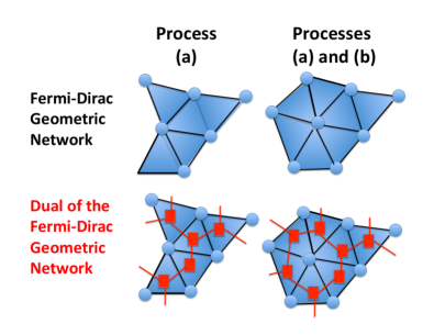
X Dual networks and Connection between the Fermi-Dirac Quantum Network and Spin Networks
Starting from the Fermi-Dirac Quantum network we can construct the dual network by mapping each triangle of the original network to a node of the dual network and every link of the original network to a link in the dual network (see Figure 23).
Each node of the dual of the Fermi-Dirac Network has degree . A link of the dual network can be saturated or unsaturated. A link of the dual network is saturated if it connects two nodes of the dual network. This happens if and only if the two corresponding triangles of the original network are glued together (i.e. they have a common link). A link of the dual network is unsaturated if it does not connect two nodes. This happens if a triangle of the original network has an unsaturated link.
As the Fermi-Dirac network grows, also the dual network grows. In the original Fermi-Dirac Network only process (a) takes place, therefore the dual network is a tree. If instead one considers the Generalized Fermi-Dirac Network, in which also process (b) takes place, the dual network contains loops (see Figure 23).
In the case in which the energies of the nodes take only integer values we can interpret the dual network as a spin network spinnet1 ; spinnet2 ; Rovelli . In fact we can associate to the link of the dual network the half-integer spin given by Eq. satisfying the Clebsch-Gordon conditions given by Eq. at each node of the dual network. Nevertheless, we note here that the quantum evolution of the proposed Fermi-Dirac network is a non-equilibrium dynamics and not an equilibrium one as usually assumed in the context of spin networks.
In the case of the Bose-Einstein Networks it is also possible to construct the dual network following a similar procedure used for constructing the dual of the Fermi-Dirac Network, but in this case the dual will not be regular, since each triangle in the Bose-Einstein network model can be linked to an arbitrarily large number of other triangles incident to the links at its boundary.
It is to mention that in the literature of quantum gravity spin networks with a causal structure have been proposed and are the so called energetic causal sets Smolin1 ; Smolin2 ; Smolin3 . It will be therefore interesting to explore further the connections between the Fermi-Dirac Networks and energetic causal sets.
Our framework is instead quite far from the spin networks used in Loop Quantum Gravity. Notably in complex quantum network geometries we do not make use of intertwines, and the network does not have relevant simple symmetries.
XI Relation to triangulations, foams, and planar graphs
Planar complex networks have already been studied in the literature in several contexts Planar ; Doro_link ; det ; Apollonian ; Aste2 ; Aste3 ; Eckmann , including the study of glass and foams, and planar complex networks.
The model most closely related to our model is the scale-free random network constructed by adding randomly triangles to links Doro_link . Nevertheless, our model does not reduce to this model for any value of the parameters. In fact also the Bose-Einstein Network for is not equivalent to this model. The difference is that in the Bose-Einstein network at , each link is not chosen randomly, but proportionally to the number of triangles already incident to it (i.e. ), according to a kind of ”preferential attachment” to the link.
Other planar scale-free network models are the pseudo-fractal scale-free network det and the Apollonian networks Apollonian . These network models are deterministic and yield scale-free networks with given power-law exponent, while the Bose-Einstein Networks are stochastic planar scale-free networks whose power-law exponent depends on the distribution and on the value of the inverse temperature .
Other models for complex networks embedded into surfaces have been recently proposed Aste2 extending approaches used already in the study of glasses and foams Aste3 ; Eckmann . In Aste2 maximal embedded graphs have been characterized using a Monte Carlo algorithm determined by an Hamiltonian which is a function of the degree of the nodes. This dynamics can explore networks embedded in surfaces of different genus, and displays a dynamical slowing down as a function of the inverse temperature of the Monte Carlo algorithm. Therefore in these simulations the ground state, ordered network is not observed, similarly to what has been observed in models of glass and foam dynamics Eckmann ; Aste3 . This approach is very different from the one proposed in the present article, although the focus is always the characterization of the network geometry. For example the phase transitions present in the Quantum Complex Network Geometries are very different from the one observed in Aste2 ; Aste3 ; Eckmann . In fact in the Complex Quantum Network Geometries the observed phase transitions are non-equilibrium phase transitions, they are determined by the quenched disorder in the network. Instead, in Aste2 ; Aste3 ; Eckmann the network has an equilibrium Hamiltonian dynamics, the ground state is well defined but there is a dynamical slow down. Moreover, in Complex Quantum Network Geometries the observed phase transitions can change the metric properties of the networks, which can go from a small-world network to a network with large diameter without changing its Euler characteristic, as in the case of the phase transition observed for Fermi-Dirac networks. Instead in Aste2 , changes from small world networks to networks with large diameter occur as a function of the Euler characteristic of the network.
XII Conclusions
In this work we have proposed to study a geometrical network evolution based on growing simplicial complexes of dimension , i.e. simplicial complexes formed by triangles. The network evolution describes the evolution of a quantum network state defined by a path integral. The quantum network states are characterized by a set of quantum occupation numbers that can be mapped to the existence of nodes, links and triangles incident to the links of the geometric network. In particular we distinguish between Fermi-Dirac network states in which the incident triangles quantum occupation number can take only values , and the Bose-Einstein quantum network state where it can take any possible integer value The Fermi-Dirac Network describes the evolution of the quantum Fermi-Dirac network state and the Bose-Einstein Network describes the evolution of the quantum Bose-Einstein network state. The average of the number of triangles exceeding one and incident to links of energy follows the Fermi-Dirac and the Bose-Einstein statistics in the Fermi-Dirac and in the Bose-Einstein Networks respectively. The Fermi-Dirac and the Bose-Einstein Networks are complex networks, including the small-world property, high clustering coefficient, exponential and scale-free degree distributions, and high modularity. The proposed network models have an emergent random geometry, since their Euler characteristic can go from (planar networks) to where are the number of nodes in the network, and can have a non-trivial distribution of the curvature . Moreover these networks can have a phase transition as a function of the external parameter called the inverse temperature. For the Fermi-Dirac network is not any more small-world and the diameter grows as a power-law of the number of nodes . For the Bose-Einstein Network undergoes a Bose-Einstein condensation, and one link acquires a finite fraction of triangles, therefore the two nodes at the two ends of the link have a finite fraction of all the links.
We believe that this model can be used to explore further the relation of complex geometries with quantum mechanics.
In the future, we plan to explore further the geometrical network model by characterizing the networks with general values of the parameter , defining the corresponding quantum state evolution
and characterizing further their topological and geometrical properties.
Moreover, we plan to study how quantum dynamical processes Ising ; BH ; BHJ ; Jesus1 ; Garneronegoogle can be affected by the structure of these networks.
Finally we plan to consider equilibrium network models describing the underlying structure of simplicial complexes and to explore the possibility to observe further structural
phase transitions in geometrical complex networks.
References
- (1) R. Albert and A.-L. Barabasi, Rev. Mod. Phys. 74, 47 (2002).
- (2) M. E. J. Newman, SIAM Review 45, 167-256 (2003).
- (3) S. Boccaletti, V. Latora, Y. Moreno, M. Chavez and D.-U. Hwang, Physics Reports 424, 175 - 308 (2006).
- (4) S.N. Dorogovtsev and J. F.F. Mendes Evolution of networks: From biological nets to the Internet and WWW (Oxford University Press,Oxford, 2003).
- (5) S. Fortunato, Phys. Rep. 486, 75 (2010).
- (6) C. Rovelli and F. Vidotto, Covariant Loop Quatum Gravity, (Cambridge University Press,Cambridge, 2015).
- (7) R. Penrose, in Quantum Theory and Beyond, (ed. T. Bastin, Cambridge University Press, Cambridge, 1971).
- (8) R. Penrose, in Magic Without Magic, (ed. J. Klauder, Freeman, San Francisco, 1972).
- (9) T.Regge, Il Nuovo Cimento Series 10, 558 (1961).
- (10) Y. Lin, L. Lu, and S.-T. Yau, Tohoku Mathematical Journal 63, 605 (2011).
- (11) Y. Lin, and S.-T. Yau, Math. Res. Lett 17 343 (2010).
- (12) F. J. Bauer, J. Jost, and S. Liu, arXiv preprint arXiv:1105.3803 (2011).
- (13) Y. Ollivier, Journal of Functional Analysis 256, 810 (2009).
- (14) O. Knill, arXiv:1202.4514 (2012).
- (15) O. Narayan, and I. Saniee, Phys. Rev. E 84, 066108 (2011).
- (16) M. Keller, Discrete & Computational Geometry 46, 500 (2011).
- (17) M. Keller, and P. Norbert, Mathematische Zeitschrift 268, 871 (2011).
- (18) Y. Higuchi, Journal of Graph Theory 38, 220 (2001).
- (19) M. Gromov, Hyperbolic groups. (Springer, New York, 1987).
- (20) W. Chen, W. Fang, G. Hu, and M. W. Mahoney, Internet Mathematics 9, 434 (2013).
- (21) E. Jonckheere, P. Lohsoonthorn, and F. Bonahon, Journal of Graph Theory 57, 157 (2008).
- (22) E. Jonckheere, M. Lou, F. Bonahon, and Y. Baryshnikov, Internet Mathematics 7, 1 (2011).
- (23) G. Petri, M. Scolamiero, I. Donato, and F. Vaccarino, PloS One 8, e66506 (2013).
- (24) G. Petri, P. Expert, F. Turkheimer, R. Carhart-Harris, D. Nutt, P.J. Hellyer, and F. Vaccarino, Journal of The Royal Society Interface 11, 20140873 (2014).
- (25) D. Taylor, F. Klimm, H. A. Harrington, M. Kramar, K. Mischaikow, M. A. Porter, and P. J. Mucha, arXiv:1408.1168 (2014).
- (26) S. N. Dorogovtsev, J. F. F. Mendes and A. N. Samukhin, Phys. Rev. E 63 062101 (2001).
- (27) S. N. Dorogovtsev,A. V. Goltsev, and J. F. F. Mendes. Phys. Rev. E 65 066122 (2002).
- (28) J. S. Andrade Jr, H. J. Herrmann, R. F. S. Andrade, and L. R. da Silva Phys. Rev. Lett. 94, 018702 (2005).
- (29) T. Aste, R. Gramatica, and T. Di Matteo, Phys. Rev. E 86, 036109 (2012).
- (30) T. Aste, T. Di Matteo, and S: T. Hyde, Physica A: Statistical Mechanics and its Applications 346, 20 (2005).
- (31) R. Kleinberg, In INFOCOM 2007. 26th IEEE International Conference on Computer Communications. IEEE, 1902, (2007).
- (32) M. Boguñá, D. Krioukov, and K. C. Claffy, Nature Physics 5, 74 (2008).
- (33) M. Boguñá, F. Papadopoulos, and D. Krioukov, Nature Commun. 1, 62 (2010).
- (34) D. Krioukov, F. Papadopoulos, M. Kitsak, A. Vahdat, and M. Boguñá, Phys. Rev. E 82, 036106 (2010).
- (35) F. Papadopoulos, M. Kitsak, M.A. Serrano, M. Boguñá, and D. Krioukov, Nature 489, 537 (2012).
- (36) J. R. Clough and T. Evans, preprint arXiv:1408.1274 (2014).
- (37) R. Albert, B. DasGupta, and N. Mobasheri, Phys. Rev. E 89, 032811 (2014).
- (38) M. Borassi, A. Chessa and G. Caldarelli, preprint arXiv:1503.03061 (2015).
- (39) A. Costa and M. Farber, arxiv:1412.5805 (2014).
- (40) D. Cohen, A. Costa, M. Farber, T. Kappeler Discrete and Computational Geometry, 47, 117 (2012).
- (41) M. Kahle, Topology of random simplicial complexes: a survey AMS Contemp. Math 620, 201 (2014).
- (42) K. Zuev, O. Eisenberg, D. Krioukov, arXiv:1502.05032 (2015).
- (43) Z. Wu, G. Menichetti, C. Rahmede and G. Bianconi, Scientific Reports 5, 10073 (2015).
- (44) D. Oriti, Reports on Progress in Physics 64, 1703 (2001).
- (45) L. Bombelli, J. Lee, D. Meyer and R. D. Sorkin, Phys. Rev. Lett. 59 (1987) 521.
- (46) M. Cortês, L. Smolin, Phys. Rev. D 90, 084007 (2014).
- (47) M. Cortês, L. Smolin, Physical Review D, 90, 044035 (2014).
- (48) M. Cortês, L. Smolin, arXiv:1407.0032 (2014).
- (49) J. Ambjorn, J. Jurkiewicz, and R. Loll, Phys. Rev. D 72, 064014 (2005).
- (50) J. Ambjorn, J. Jurkiewicz, and R. Loll Phys. Rev. Lett. 93, 131301 (2004).
- (51) D. Krioukov, M. Kitsak, R. S. Sinkovits, D. Rideout, D. Meyer, M. Boguñá, Scientific Reports 2, 793 (2012).
- (52) J. A. Wheeler, Quantum theory and gravitation (ed. A. R. Marlov, Academic Press, New York, 1980).
- (53) P.E. Gibbs, arXiv preprint hep-th/9506171 (1995).
- (54) D. Meschini, M. Lehto, and J. Piilonen, Studies in History and Philosophy of Science Part B: Studies in History and Philosophy of Modern Physics, 36, 435 (2005).
- (55) F. Antonsen, International journal of theoretical physics, 33, 11895 (1994).
- (56) T. Konopka, F. Markopoulou, S. Severini, Phys. Rev. D 77, 104029 (2008).
- (57) A. Hamma, F. Markopoulou, S. Lloyd, F. Caravelli, S. Severini, and K. Markström, Phys. Rev. D 81, 104032 (2010).
- (58) G. Bianconi, A.-L. Barabási, EPL 54, 436 (2001).
- (59) G. Bianconi and A.-L. Barabási, Phys. Rev. Lett. 86, 5632 (2001).
- (60) G. Bianconi, Phys. Rev. E 66, 036116 (2002).
- (61) G. Bianconi, Phys. Rev. E 66, 056123 (2002).
- (62) G. Bianconi, EPL 71, 1029 (2005).
- (63) D. Garlaschelli, M. I. Loffredo, Phys. Rev. Lett. 102, 038701 (2009).
- (64) O.Mülken, and A. Blumen, Physics Reports 502, 37 (2011).
- (65) M. B. Plenio and S. F. Huelga, New J. Phys. 10, 113019 (2008).
- (66) S. Perseguers, M. Lewenstein, A. Acín, J. I. Cirac, Nature Physics 6, 539 (2010).
- (67) M. Faccin, P. Migdal, T. H. Johnson, V. Bergholm, J. D. Biamonte, Phys. Rev. X 4, 041012 (2014).
- (68) M. Faccin, T. Johnson, J. Biamonte, S. Kais, and P.Migdal, Phys. Rev. X 3, 041007 (2013).
- (69) Note that throughout the paper we give physically inspired names to mathematical quantities describing the complex quantum network evolution, but no indication is given to an experimental implementation of the complex quantum network geometries or of the quantum network states.
- (70) D. J. Watts, and S. Strogatz, Nature 393, 440 (1998).
- (71) A. -L. Barabási, and R. Albert, Science 286, 509 (1999).
- (72) K. Zhao, A. Halu, S. Severini, and G. Bianconi Phys. Rev. E 84, 066113 (2011).
- (73) K. Anand, G. Bianconi, S. Severini, Phys. Rev. E 83, 036109 (2011).
- (74) S. Garnerone, P. Giorda, P. Zanardi, New J. Phys. 14, 013011 (2012).
- (75) L. Han, F. Escolano, E. R. Hancock, and R. C. Wilson, Pattern Recognition Letters 33, 1958 (2012).
- (76) M. E. J. Newman, and M. Girvan, Phys. Rev. E 69, 026113 (2004).
- (77) V. D. Blondel, J. L. Guillaume, R. Lambiotte, and E. Lefebvre Journal of Statistical Mechanics: Theory and Experiment, P10008 (2008).
- (78) E. Ravasz, A. L. Somera, D. A. Mongru, Z. N. Oltvai, and A.-L. Barabási, Science 297, 1551 (2002).
- (79) M. Kardar,Statistical Physics of Particles (Cambridge University Press, Cambridge 2007)
- (80) P. Bialas, Z. Burda, J. Jurkiewicz, and A. Krzywicki, Phys. Rev. E 67, 066106 (2003).
- (81) P. Bialas, Z. Burda, and D. Johnston, Nuclear Physics B 542, 413 (1999).
- (82) G. Bianconi, Phys. Rev. E 85, 061113 (2012).
- (83) A. Halu, L. Ferretti, A. Vezzani and G. Bianconi, EPL 99 18001 (2012).
- (84) A. Halu, S. Garnerone, A. Vezzani, and G. Bianconi, Phys. Rev. E 87, 022104 (2013).
- (85) E. Sanchez-Burillo, J. Duch, J. Gomez-Gardeñes, D. Zueco, Scientific Reports 2,605 (2012).
- (86) S. Garnerone, P. Zanardi, and D. A. Lidar, Phys. Rev. Lett. 108, 230506 (2012).
- (87) E. Brézin, C. Itzykson, G. Parisi and J. B. Zuber, Commun. Math. Phys. 59, 35 (1978).
- (88) T. Aste and D. Sherrington, J. Phys. A 32 7049 (1999).
- (89) J.-P. Eckmann, J. Stat. Phys. 129, 289 (2007).