Template-based Monocular 3D Shape Recovery using Laplacian Meshes
Abstract
We show that by extending the Laplacian formalism, which was first introduced in the Graphics community to regularize 3D meshes, we can turn the monocular 3D shape reconstruction of a deformable surface given correspondences with a reference image into a much better-posed problem. This allows us to quickly and reliably eliminate outliers by simply solving a linear least squares problem. This yields an initial 3D shape estimate, which is not necessarily accurate, but whose 2D projections are. The initial shape is then refined by a constrained optimization problem to output the final surface reconstruction.
Our approach allows us to reduce the dimensionality of the surface reconstruction problem without sacrificing accuracy, thus allowing for real-time implementations.
Index Terms:
Deformable surfaces, Monocular shape recovery, Laplacian formalism1 Introduction
Shape recovery of deformable surfaces from single images is inherently ambiguous, given that many different configurations can produce the same projection. In particular, this is true of template-based methods, in which a reference image of the surface in a known configuration is available and point correspondences between this reference image and an input image in which the shape is to be recovered are given.
One approach is to compute a 2D warp between the images and infer a 3D shape from it, which can be done pointwise and in closed form [1]. The quality of the recovered 3D shape then depends on the quality of the 2D warp, which does not necessarily account for the 3D nature of the deformations and the constraints it imposes. This problem can be avoided by computing the 3D shape directly from the correspondences, which amounts to solving a degenerate linear system and requires either reducing the number of degrees of freedom or imposing additional constraints [2]. The first can be achieved by various dimensionality reduction techniques [3, 4] while the second often involves assuming the surface to be either developable [5, 6, 7] or inextensible [8, 9, 10, 4]. These two approaches are sometimes combined and augmented by introducing additional sources of information such as shading or textural clues [11, 12] or physics-based constraints [13]. The resulting algorithms usually require solving a fairly large optimization problem and, even though it is often well behaved or even convex [10, 8, 14, 15, 4], it remains computationally demanding. Closed-form approaches to directly computing the 3D shape from the correspondences have been proposed [16, 12] but they also involve solving very large systems of equations and making more restrictive assumptions than the optimization-based ones, which can lower performance [4].
Here, we show that, by extending the Laplacian formalism first introduced in the Graphics Community [17, 18, 19] and introducing a novel regularization term designed to minimize curvature changes from the potentially non-planar reference shape, we can turn the large degenerate linear system mentioned above into a non-degenerate one. We further show that the resulting least-squares problem can be reduced to a much smaller one by expressing all vertex coordinates as linear combinations of those of a small number of control vertices, which considerably increases computational efficiency at no loss in reconstruction accuracy.
In other words, instead of performing a minimization involving many degrees of freedom or solving a large system of equations, we end up simply solving a very compact linear system. This yields an initial 3D shape estimate, which is not necessarily accurate, but whose 2D projections are. In practice, this is extremely useful to quickly and reliably eliminate erroneous correspondences. We can then achieve better accuracy than the methods of [4, 10, 1] on both planar and non-planar surfaces by enforcing simple inextensibility constraints. This is done by optimizing over a small number of variables, thereby lowering the computational complexity and allowing for a real-time implementation.
In short, our contribution is a novel approach to regularizing and reducing the dimensionality of the surface reconstruction problem. It does not require either an estimate of the rigid transformation with respect to the reference shape or access to training data or material properties, which may be unavailable or unknown. Furthermore, this is achieved without sacrificing accuracy and can handle arbitrarily large deformations and generic objective functions, which is beyond what earlier Laplacian formalisms were designed to do. Each one of these features can be found in isolation in other approaches but ours brings them all together in a unified framework. It was first introduced in a conference paper [20] and is validated more thoroughly here.
In the remainder of this paper, we first review existing approaches and remind the reader how the problem can be formulated as one of solving a linear but degenerate system of equations, as we did in earlier work [2]. We then introduce our extended Laplacian formalism, which lets us transform the degenerate linear system into a non-degenerate one and if necessary make it smaller for better computational efficiency. Finally, we present our results and compare them against state-of-the-art methods [4, 10, 1].
2 Related Work
Reconstructing the 3D shape of a non-rigid surface from a single input image is a severely under-constrained problem, even when a reference image of the surface in a different but known configuration is available. This is the problem we address here, as opposed to recovering the shape from sequences as in many recent monocular Non-Rigid Structure from Motion methods such as [21, 22].
When point correspondences can be established between the reference and input images, one can compute a 2D warp between the images and infer a 3D shape from it, which can be done in closed form and pointwise [1]. However, the accuracy of the recovered shape can be affected by the fact that the 2D warp may not take into account he constraints that arise from the 3D nature of the surface and its deformations.
An alternative is therefore to go directly from correspondences to 3D shape by solving an ill-conditioned linear-system [2], which requires the introduction of additional constraints to make it well-posed. The most popular ones involve preserving Euclidean or Geodesic distances as the surface deforms and are enforced either by solving a convex optimization problem [10, 8, 23, 9, 14, 15, 4, 24] or by solving in closed form sets of quadratic equations [16, 12]. The latter is typically done by linearization, which results in very large systems and is no faster than minimizing a convex objective function, as is done in [4] which has been shown to be an excellent representative of this class of techniques. The results can then be improved by imposing appropriate physics-based constraints [13] via non-linear minimization, but that requires some knowledge of the physical properties that may not be available.
The complexity of the problem can be reduced using a dimensionality reduction technique such as Principal Component Analysis (PCA) to create morphable models [25, 3, 26], modal analysis [12, 14], Free Form Deformations (FFDs) [10], or 3D warps [27]. One drawback of PCA and modal analysis is that it requires either training data or sufficient knowledge of the surface properties to compute a stiffness matrix, neither of which may be forthcoming. Another is that the modal deformations are expressed with respect to a reference shape, which must be correctly positioned. This makes it necessary to introduce additional rotation and translation parameters into the computation. This complicates the computations because the rotations cannot be treated as being linear unless they are very small. The FFD approach [10] avoids these difficulties and, like ours, relies on parameterizing the surface in terms of control points. However, its affine-invariant curvature-based quadratic regularization term is designed to preserve local structures and planarity. For non-planar surfaces, it tends to flatten the surface in areas with only limited image information. By contrast, our approach naturally handles non-planar reference surfaces, tends to preserve curvature, and its control vertices can be arbitrarily placed. This makes it closer to earlier ones to fitting 3D surfaces to point clouds that also allow arbitrary placement of the control points by using Dirichlet Free Form Deformations [28] or, more recently, sets of affine transforms [29]. These approaches, however, also require regularization of the control points if they are to be used to fit surfaces to noisy data.
In short, none of these dimensionality reduction methods allows both orientation-invariant and curvature-preserving regularization. To do both simultaneously, we took our inspiration from the Laplacian formalism presented in [17] and the rotation invariant formulation of [18], which like ours involves introducing virtual vertices. In both these papers, the mesh Laplacian is used to define a regularization term that tends to preserve the shape of a non-planar surface.
In [19], it is shown that explicitly adding the virtual vertices is not necessary to achieve similar or even better results. In our work, we go one step further by not only introducing a rotation invariant regularization term expressed as a linear combination of the vertex coordinates but showing that these coordinates can themselves be written as a linear function of those of a subset of control vertices while preserving rotation invariance. Furthermore, in [18], the regularization term involves minimizing the magnitude of the local deformations, which favors small deformations. By contrast, our approach only penalizes curvature changes and can accommodate arbitrarily large deformations.
3 Linear Problem Formulation
As shown in [2], but for the sake of completeness we show again that given point correspondences between a reference image in which the 3D shape is known and an input image, recovering the new shape in this image amounts to solving a linear system.
Let be the 3D coordinates of the vertex of the -vertex triangulated mesh representing the surface, be the intrinsic camera matrix, be a 3D point lying on facet . One can represent in the barycentric coordinates of : , where are the three vertices of . The fact that projects to the 2D image point can be expressed by
| (1) |
where is the homogeneous component. Since can be expressed in terms of the vertex coordinates using the last row of the above equation, we can rewrite Eq. 1 to be
| (2) |
with
| (3) |
where are the first two rows, and is the third one of . Given correspondences between 3D reference surface locations and 2D image points, we obtain linear equations which can be jointly expressed by a linear system
| (4) |
and is a matrix obtained by concatenating the matrices. In practice, the sum of squares of successive elements of the vector are squared distances in the direction parallel to the image-plane between the line-of-sight defined by a feature point and its corresponding 3D point on the surface. A solution of this system defines a surface such that 3D feature points that project to specific locations in the reference image project at corresponding locations in the input image. Solving this system in the least-squares sense therefore yields surfaces, up to a scale factor, for which the overall reprojection error is small.
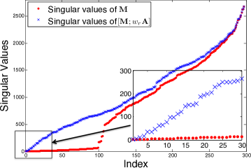
The difficulty comes from the fact that, for all practical purposes, is rank deficient as shown in Fig. 2(a), with at least one third of its singular values being extremely small with respect to the other two thirds even when there are many correspondences. This is why the inextensibility constraints, as mentioned in Section 2, will be introduced.
A seemingly natural way to address this issue is to introduce a linear subspace model and to write surface deformations as linear combinations of relatively few basis vectors. This can be expressed as
| (5) |
where is the coordinate vector of Eq. 4, is the matrix whose columns are the basis vectors typically taken to be the eigenvectors of a stiffness matrix, and is the associated vectors of weights . Injecting this expression into Eq. 4 and adding a regularization term yields a new system
| (6) |
which is to be solved in the least squares sense, where is a diagonal matrix whose elements are the eigenvalues associated to the basis vectors, and is a regularization weight. This favors basis vectors that correspond to the lowest-frequency deformations and therefore enforces smoothness.
In practice, the linear system of Eq. 6 is better posed than the one of Eq. 4. But, because there are usually several smooth shapes that all yield virtually the same projection, its matrix still has a number of near zero singular values. As a consequence, additional constraints still need to be imposed for the problem to become well-posed. An additional difficulty is that, because rotations are strongly non-linear, this linear formulation can only handle small ones. As a result, the reference shape defined by must be roughly aligned with the shape to be recovered, which means that a global rotation must be computed before shape recovery can be attempted.
In the remainder of this paper, we will show that we can reduce the dimensionality in a different and rotation-invariant way.
4 Laplacian Formulation
In the previous section, we introduced the linear system of Eq. 4, which is so ill-conditioned that we cannot minimize the reprojection error by simply solving it. In this section, we show how to turn it into a well-conditioned system using a novel regularization term and how to reduce the size of the problem for better computational efficiency.
 |
 |
| (a) | (b) |
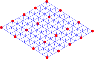
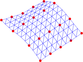
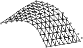
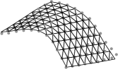
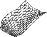
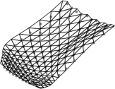
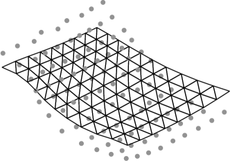
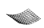
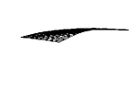
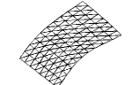
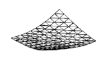
To this end, let us assume we are given a reference shape as in Fig. 1(a), which may or may not be planar and let be the coordinate vector of its vertices. We first show that we can define a regularization matrix such that , with being the coordinate vector of Eq. 4, when up to a rigid transformation. In other words, penalizes non-rigid deformations away from the reference shape but not rigid ones. The ill-conditioned linear system of Eq. 4 is augmented with the regularization term to obtain a much better-conditioned linear system
| (7) |
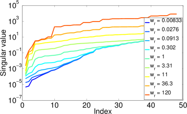
where is a scalar coefficient defining how much we regularize the solution. Fig. 2(a) illustrates this for a specific mesh. In the result section, we will see that this behavior is generic and that we can solve this linear system for all the reference meshes we use in our experiments.
 |
 |
| (a) | (b) |
We then show that, given a subset of mesh vertices whose coordinates are
| (8) |
if we force the mesh both to go through these coordinates and to minimize , we can define a matrix that is independent of the control vertex coordinates and such that
| (9) |
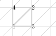
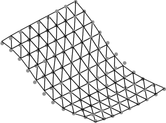
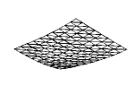
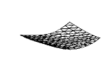
In other words, we can linearly parameterize the mesh as a function of the control vertices’ coordinates, as illustrated in Fig. 1, where the control vertices are shown in red and (a) is the reference shape and (b) is a deformed shape according to Eq. 9. Injecting this parameterization into Eq. 7 yields a more compact linear system
| (10) |
which similarly can be solved in the least-square sense up to a scale factor by finding the eigenvector corresponding to the smallest eigenvalue of the matrix , in which
| (11) |
We fix the scale by making the average edge-length be the same as in the reference shape. This problem is usually sufficiently well-conditioned as will be shown in Section 5.1.5. Its solution is a mesh whose projection is very accurate but whose 3D shape may not be because our regularization does not penalize affine deformations away from the reference shape. In practice, we use this initial mesh to eliminate erroneous correspondences. We then refine it by solving
| (12) |
where are inextensibility constraints that prevent Euclidean distances between neighboring vertices to grow beyond a bound, such as their geodesic distance in the reference shape. We use inequality constraints because, in high-curvature areas, the Euclidean distance becomes smaller than the geodesic distance. These are exactly the same constraints as those used in [4], against which we compare ourselves below. The inequality constraints are reformulated as equality constraints with additional slack variables whose norm is penalized to prevent lengths from becoming too small and the solution from shrinking to the origin [30]. This makes it unnecessary to introduce the depth constraints of [4]. As shown in Appendix B, this non-linear minimization step is important to guarantee that not only are the projections correct but also the actual 3D shape.
4.1 Regularization Matrix
We now turn to building the matrix such that and when is a rigidly transformed version of . We first propose a very simple scheme for the case when the reference shape is planar and then a similar, but more sophisticated one, when it is not.
 |
 |
 |
| (a) | (b) | (c) |
4.1.1 Planar Reference Shape
Given a planar triangular mesh that represents a reference surface in its reference shape, consider every pair of facets that share an edge, such as those depicted by Fig. 3(a). They jointly have four vertices to . Since they lie on a plane, whether or not the mesh is regular, one can always find a unique set of weights , , and such that
| (13) | |||||
up to a sign ambiguity, which can be resolved by simply requiring the first weight to be positive. The first equation in Eq. 13 applies for each of three spatial coordinates . To form the matrix, we first generate a matrix for a single coordinate component. For every facet pair , let be the indices of four corresponding vertices. The values at row , columns of are taken to be . All remaining elements are set to zero and the matrix is , that is the Kronecker product with a identity matrix.
We show in Appendix A that when is an affine transformed version of the reference mesh and that is invariant to rotations and translations. The first equality of Eq. 13 is designed to enforce planarity while the second guarantees invariance. The third equality is there to prevent the weights from all being zero. The more the mesh deviates from an affine transformed version of the reference mesh, the more the regularization term penalizes.
4.1.2 Non-Planar Reference Shape
When the reference shape is non-planar, there will be facets for which we cannot solve Eq. 13. As in [18], we extend the scheme described above by introducing virtual vertices. As shown in Fig. 3(c), we create virtual vertices at above and below the center of each facet as a distance controlled by the scale parameter . Formally, for each facet , and , its center and its normal , we take the virtual vertices to be
| (14) |
where the norm of is approximately equal to the average edge-length of the facet’s edges. These virtual vertices are connected to vertices of their corresponding mesh facet and virtual vertices of the neighbouring facets on the same side, making up the blue tetrahedra of Fig. 3(c).
Let be the coordinate vector of the virtual vertices only, and the coordinate vector of both real and virtual vertices. Let be similarly defined for the reference shape. Given two tetrahedra that share a facet, such as the red and green ones in Fig. 3(c), and the five vertices to they share, we can now find weights to such that
| (15) | |||||
The three equalities of Eq. 15 serve the same purpose as those of Eq. 13. We form a matrix by considering all pairs of tetrahedra that share a facet, computing the to weights that encode local linear dependencies between real and virtual vertices, and using them to add successive rows to the matrix, as we did to build the matrix in the planar case. One can again verify that and that is invariant to rigid transformations of . In our scheme, the regularization term can be computed as
| (16) |
if we write as where has three times as many columns as there are real vertices and as there are virtual ones. Given the real vertices , the virtual vertex coordinates that minimize the term of Eq. 16 is
| (17) | |||||
where . In other words, this matrix is the regularization matrix we are looking for and its elements depend only on the coordinates of the reference vertices and on the scale parameter chosen to build the virtual vertices.
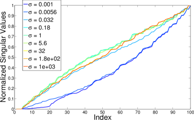
To study the influence of the scale parameter of Eq. 14, which controls the distance of the virtual vertices from the mesh, we computed the matrix and its singular values for a sail shaped mesh and many values. For each , we normalized the singular values to be in the range . As can be seen in Fig. 2(b), there is a wide range of for which the distribution of singular values remains practically identical. This suggests that has limited influence on the numerical character of the regularization matrix. In all our experiments, we set to and were nevertheless able to obtain accurate reconstructions of many different surfaces with very different physical properties.
4.2 Linear Parameterization
We now show how to use our regularization matrix to linearly parameterize the mesh using a few control vertices. As before, let be the total number of vertices and the number of control points used to parameterize the mesh. Given the coordinate vector of these control vertices, the coordinates of the minimum energy mesh that goes through the control vertices and minimizes the regularization energy can be found by minimizing
| (18) |
where is the regularization matrix introduced above and is a matrix containing ones in columns corresponding to the indices of control vertices and zeros elsewhere. We prove below that, there exists a matrix whose components can be computed from and such that
| (19) |
if is a solution to the minimization problem of Eq. 18.
To prove this without loss of generality, we can order the coordinate vector so that those of the control vertices come first. This allows us to write all coordinate vectors that satisfy the constraint as
| (20) |
where . Let us rewrite the matrix as
| (21) |
where and have and columns, respectively. Solving the problem of Eq. 18, becomes equivalent to minimizing
| (22) | |||||
| (25) |
Therefore,
| (26) |
is the matrix of Eq. 19 under our previous assumption that the vertices were ordered such that the control vertices come first.
4.3 Rejecting Outliers
To handle outliers in the correspondences, we iteratively perform the unconstrained optimization of Eq. 10 starting with a relatively high regularization weight and reducing it by half at each iteration. Given a current shape estimate, we project it on the input image and disregard the correspondences with higher reprojection error than a pre-set radius and reduce it by half for the next iteration. Repeating this procedure a fixed number of times results in an initial shape estimate and provides inlier correspondences for the more computationally demanding constrained optimization that follows.
Even though the minimization problem we solve is similar to that of [4], this two-step outlier rejection scheme brings us a computational advantage. In the earlier approach, convex but nonlinear minimization had to be performed several times at each iteration to reject the outliers whereas here we repeatedly solve a linear least squares problem instead. Furthermore, the final non-linear minimization of Eq. 12 involves far fewer variables since the control vertices typically form a small subset of all vertices, that is, .
5 Results
In this section, we first compare our approach to surface reconstruction from a single input image given correspondences with a reference image against the recent methods of [10, 4, 1], which are representative of the current state-of-the-art. We then present a concrete application scenario and discuss our real-time implementation of the approach. We supply the corresponding videos as supplementary material. They are also available on the web 111http://cvlabwww.epfl.ch/~fua/tmp/laplac along with the Matlab code that implements the method. 222http://cvlab.epfl.ch/page-108952-en.html
5.1 Quantitative Results on Real Data
To provide quantitative results both in the planar and non-planar cases we use five different sequences for which we have other means besides our single-camera approach to estimate 3D shape. We first describe them and then present our results. Note that we process every single image individually and do not enforce any kind of temporal consistency to truly compare the single-frame performance of all four approaches.
 |
 |
 |
 |
 |
 |
 |
 |
 |
 |
 |
 |
 |
 |
 |
 |
| (a) | (b) | (c) | (d) |
 |
 |
 |
 |
 |
 |
 |
 |
 |
 |
 |
 |
| (a) | (b) | (c) |
5.1.1 Sequences, Templates, and Validation
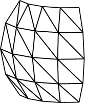
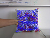
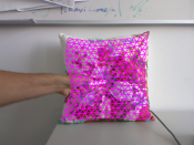
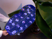
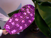
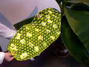
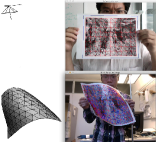
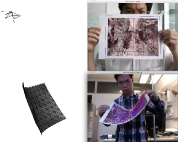
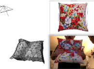
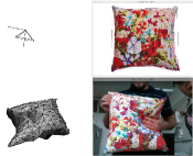
We acquired four sequences using a Kinect, whose RGB camera focal length is about 528 pixels. We show one representative image from each dataset in Figs. 4 and 5. We performed the 3D reconstruction using individual RGB images and ignoring the corresponding depth images. We used these only to build the initial template from the first frame of each sequence and then for validation purposes. The specifics for each one are provided in Table I.
For the paper and apron of Fig. 4, we used the planar templates shown in the first two rows of Fig. 8 and for the cushion and banana leaf of Fig. 5 the non-planar ones shown in next two rows of the same figure. For the paper, cushion, and leaf, we defined the template from the first frame, which we took to be our reference image. For the apron, we acquired a separate image in which the apron lies flat on the floor so that the template is flat as well, which it is not in the first frame of the sequence, so that we could use the method of [10] in the conditions it was designed for.
| Dataset | # frames | # vertices | # facets | Planar |
|---|---|---|---|---|
| Paper | 192 | 99 | 160 | Yes |
| Apron | 160 | 169 | 288 | Yes |
| Cushion | 46 | 270 | 476 | No |
| Leaf | 283 | 260 | 456 | No |
| Sail | 6 | 66 | 100 | No |
To create the required correspondences, we used either SIFT [31] or Ferns [32] to establish correspondences between the template and the input image. We ran our method and three others [10, 1, 4] using these correspondences as input to produce results such as those depicted by Figs. 4 and 5.
As stated above, we did not use the depth-maps for reconstruction purposes, only for validation purposes. We take the reconstruction accuracy to be the average distance of the reconstructed 3D vertices to their projections onto the depth images, provided they fall within the target object. Otherwise, they are ignored. Since we do the same for all four methods we compare, comparing their performance in terms of these averages and corresponding variances is meaningful and does not introduce a bias.
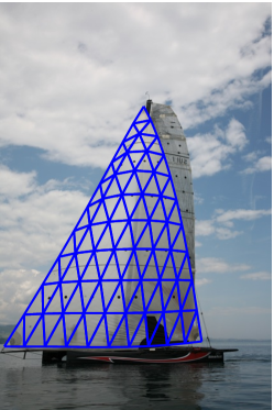
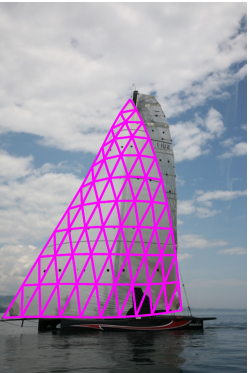
The last dataset is depicted by Fig. 6. It consists of 6 pairs of images of a sail, which is a much larger surface than the other four and would be hard to capture using a Kinect-style sensor. The images were acquired by two synchronized cameras whose focal lengths are about 6682 pixels, which let us accurately reconstruct the 3D positions of the circular black markers by performing bundle-adjustment on each image pair. As before we took the first image captured by the first camera to be our reference image and established correspondences between the markers it contains and those seen in the other images. We also established correspondences between markers within the stereo pairs and checked them manually. We then estimated the accuracy of the monocular reconstructions in terms of the distances of the estimated markers’ 3D positions to those obtained from stereo.
 |
 |
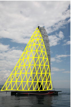 |
 |
 |
 |
| (a) | (b) | (c) |
The 3D positions of the markers used to evaluate the reconstruction error are estimated from the stereo images up to an unknown scale factor: This stems from the fact that both the relative pose of one stereo camera to the other and the 3D positions of the markers are unknown and have to be estimated simultaneously. However, once a stereo reconstruction of the markers has been obtained, fitting a mesh to those markers lets us estimate an approximate scale by assuming the total edge length of the fitted mesh to be that of the reference mesh. However it is not accurate and, for evaluation purposes, we find a scale factor within the range that we apply to each one of the monocular reconstructions so as to minimize the mean distance between the predicted 3D marker positions of the monocular reconstructions and the 3D positions obtained from stereo.
5.1.2 Robustness to Erroneous Correspondences
 |
 |
 |
 |
 |
 |
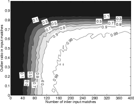
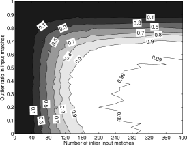
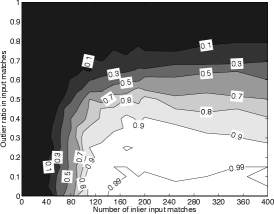
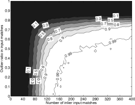
| (a) Ours | (b) Tran et al. ECCV 2012 [33] | (c) Pizarro et al. IJCV 2012 [34] |
We demonstrate the robustness of our outlier rejection scheme described in Section 4.3 for both planar and non-planar surfaces. We also compare our method against two recent approaches to rejecting outliers in deformable surface reconstruction [34, 33] whose implementations are publicly available. Alternatives include the older M-estimator style approaches of [35, 36], which are comparable in matching performance on the kind of data we use but slower [33]. A more recent method [37] involves detecting incorrect correspondences using local isometry deformation constraints by locally performing intensity-based dense registration. While potentially effective, this algorithm requires several seconds per frame, which is prohibitive for real-time implementation purpose.
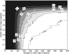
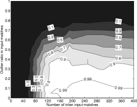
We used one image from both the paper and the cushion datasets in which the surfaces undergo large deformations, as depicted by the first row of Figs. 4 and 5. We used both the corresponding Kinect point cloud and SIFT correspondences to reconstruct a mesh that we treated as the ground truth. We then synthesized approximately 600’000 sets of correspondences by synthetically generating 10 to 400 inlier correspondences spread uniformly across the surface, adding a zero mean Gaussian noise with standard deviation of 1 pixel to the corresponding pixel coordinates, and introducing proportions varying from to of randomly spread outlier correspondences.
We ran our algorithm with regularly sampled control vertices on each one of these sets of correspondences. To ensure a fair comparison of outlier rejection capability in the context of deformable surface reconstruction, also because [33] was designed only for outlier rejection, and the implementation of [34] only performs outlier rejection, we used the set of inlier correspondences returned by these methods to perform surface registration using our method assuming that all input correspondences are inliers. For [34, 33], we used the published parameters except for the threshold used to determine if a correspondence is an inlier or an outlier and the number of RANSAC iterations. We tuned the threshold manually and used 5 times more RANSAC iterations than the suggested default value for [33] to avoid a performance drop when dealing with a large proportion of outliers. Note that choosing the threshold parameter for [33] is non trivial because the manifold of inlier correspondences is not exactly a 2-D affine plane, as assumed in [33].
We evaluated the success of these competing methods in terms of how often at least of the reconstructed 3D mesh vertices project within pixels of where they should. Fig. 7 depicts the success rates according to this criterion over many trials as a function of the total number of inliers and the proportion of outliers. Our method is comparable to [33] on the cushion dataset and better on the paper dataset. It is much better than [34] on both datasets. Our algorithm requires approximately 200 inlier correspondences to guarantee the algorithm will tolerate high ratios of outliers with 0.99 probability. Rejecting outliers and registering images on approximately 600’000 set of synthesized correspondences on the paper and cushion dataset, respectively, took our method 11.73 (14.80) hours i.e. 0.070 (0.089) second per frame, took [33] 44.02 (48.83) hours i.e. 0.26 (0.29) second per frame, and took [34] 197.46 (201.23) hours i.e. 1.18 (1.21) second per frame.
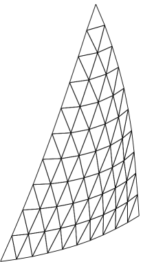
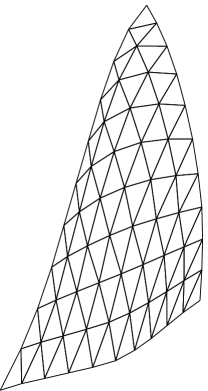
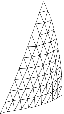
5.1.3 Control Vertex Configurations
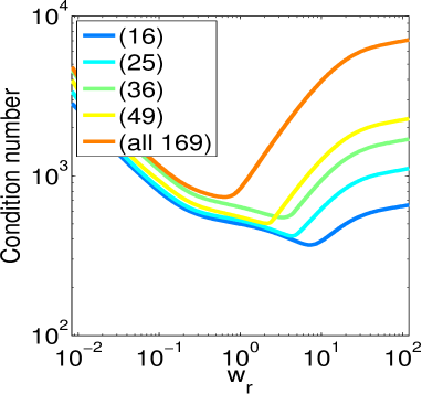
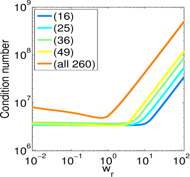
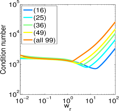
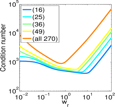
| (16) | (25) | (36) | (49) | (99) | (16) | (25) | (36) | (49) |
| (16) | (25) | (36) | (49) | (169) | (16) | (25) | (36) | (49) |
| (16) | (25) | (36) | (49) | (270) | (16) | (25) | (36) | (49) |
| (16) | (25) | (36) | (49) | (260) | (16) | (25) | (36) | (49) |
| (8) | (12) | (18) | (27) | (66) | (8) | (12) | (18) | (27) |
One of the important parameters of our algorithm is the number of control vertices to be used. For each one of the five datasets, we selected four such numbers and hand-picked regularly spaced sets of control vertices of the right cardinality. We also report the results using all mesh vertices as control vertices. The left side of Fig. 8 depicts the resulting configurations.
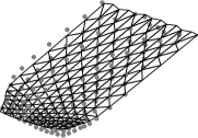
To test the influence of the positioning of the control vertices, for each sequence, we also selected control vertex sets of the same size but randomly located, such as those depicted on the right side of Fig. 8. We did this six times for each one of the four templates and each possible number of control vertices.
In other words, we tested 29 different control vertex configurations for each sequence.
5.1.4 Comparative Accuracy of the Four Methods
We fed the same correspondences, which contain erroneous ones, to implementations, including the outlier rejection strategy, provided by the authors of [10, 4, 1] to compare against our method. In the case of [1], we computed the 2D image warp using the algorithm of [34] as described in the section Experimental Results of [1].
As discussed above, for the kinect sequences, we characterize the accuracy of their respective outputs in terms of the mean and variance of the distance of the 3D vertices reconstructed from the RGB images to their projections onto the depth images. For the sail images, we report the mean and variance of the distance between 3D marker positions computed either monocularly or using stereo, under the assumption that the latter are more reliable.
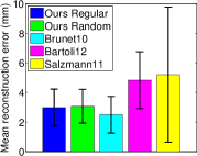
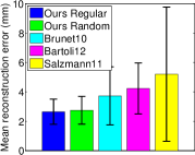
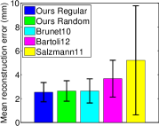
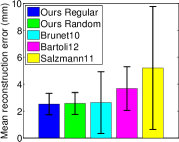
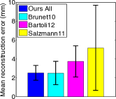
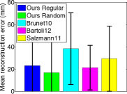
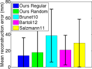
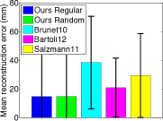
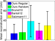
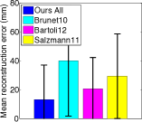
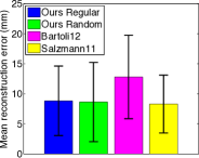
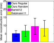
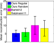
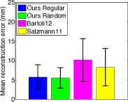
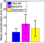
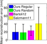
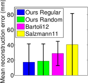
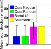
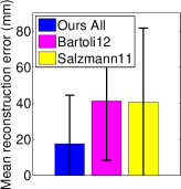
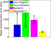
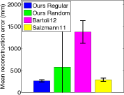
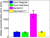
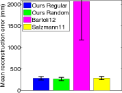
In Fig. 9, we plot these accuracies when using planar templates to reconstruct the paper and apron of Fig. 4. The graphs are labeled as
-
•
Ours Regular and Ours Random when using our method with either the regular or randomized control vertex configurations of Fig. 8. They are shown in blue and green respectively. In the case of the randomized configurations, we plot the average results over six random trials. We denote our results as Ours All when all mesh vertices are used as control vertices.
- •
The numbers below the graphs denote the number of control vertices we used. For a fair comparison, we used the same number of control vertices to run the method of [10] and to compute the 2D warp required by the method of [1]. The algorithm of [4] does not rely on control vertices since it operates directly on the vertex coordinates. This means it depends on far more degrees of freedom than all the other methods and, for comparison purposes, we depict its accuracy by the same yellow bar in all plots of any given row.
5.1.5 Analysis
Our approach performs consistently as well or better than all the others when we use enough control vertices arranged in one of the regular configurations shown on the left side of Fig. 8. This is depicted by the blue bars in the four right-most columns of Figs. 9 and 10. Even when we use too few control vertices, we remain comparable to the other methods, as shown in the first columns of these figures.
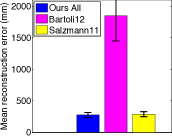
More specifically, in the planar case, our closest competitor is the method of [10]. We do approximately the same on the paper but much better on the apron. In the non-planar case that [10] is not designed to handle and when using enough control vertices, we outperform the other two methods on the cushion and the leaf and perform similarly to [4] on the sail.
As stated above, these results were obtained using regular control vertex configurations and are depicted by blue bars in Figs. 9 and 10. The green bars in these plots depict the results obtained using randomized configurations such as those shown on the right side of Fig. 8. Interestingly, they are often quite similar, especially for larger numbers of control vertices. This indicates the relative insensitivity of our approach to the exact placement of the control vertices. In fact, we attempted to design an automated strategy for optimal placement of the control vertices but found it very difficult to consistently do better than simply spacing them regularly, which is also much simpler.
Note that our linear subspace parameterization approach to reducing the dimensionality of the problem does not decrease the reconstruction accuracy when enough control vertices are used. We interpret this to mean that the true surface deformations lie in a lower dimensional space than the one spanned by all the vertices’ coordinates.
 |
 |
 |
 |
 |
| (16) | (25) | (36) | (49) | (99) |
 |
 |
 |
 |
 |
| (16) | (25) | (36) | (49) | (169) |
 |
 |
 |
 |
 |
| (16) | (25) | (36) | (49) | (270) |
 |
 |
 |
 |
 |
| (16) | (25) | (36) | (49) | (260) |
 |
 |
 |
 |
 |
| (8) | (12) | (18) | (27) | (66) |
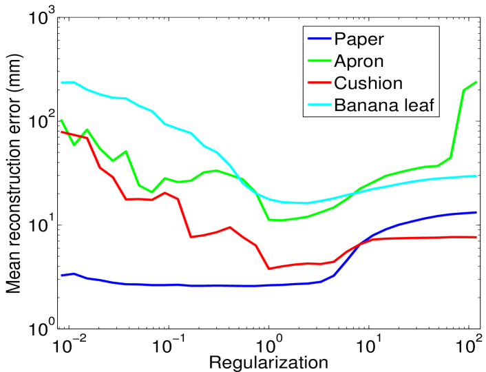
All these experiments were carried out with a regularization weight of in Eq. 12. To characterize the influence of this parameter, we used the control vertex configuration that yielded the best result for each dataset and re-ran the algorithm with the same input correspondences but with 33 different logarithmically distributed values of ranging from to . Fig. 11 depicts the results and indicates that values ranging from to all yield similar results.
 |
 |
 |
 |
 |
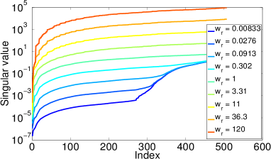 |
Fig. 12 illustrates how well- or ill-conditioned the linear system of Eq. 10 is depending on the value of . We plot condition numbers of in Eq. 11, averaged over several examples, as a function of for all the regular control-vertex configurations we used to perform the experiments described above on the four kinect sequences. We also show the singular values of , also averaged over several examples, for two different configurations of the control vertices in the apron case. Note that the best condition numbers are obtained for values of between and , which is consistent with the observation made above that these are good default values to use for the regularization parameter. This can be interpreted as follows: For very small values of , the term dominates and there are many shapes that have virtually the same projections. For very large values of , the term dominates in Eq. 10 and many shapes that are rigid transformations of each other have virtually the same deformation energy. The best compromise is therefore for intermediate values of .
5.2 Application Scenario
In this section, we show that our approach can be used to address a real-world problem, namely modeling the deformations of a baseball as it hits a bat. We obtained from Washington State University’s Sport Science Laboratory 7000 frames-per-second videos such as the one of Fig. 13, which shows the very strong deformation that occurs at the moment of impact. The camera focal length is about 2853 pixels. In this specific case, the ball was thrown at 140 mph by a launcher against a half cylinder that serves as the bat to study its behavior.
 |
 |
 |
 |
 |
 |
 |
 |
 |
 |
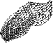
We take the reference frame to be the first one where the ball is undeformed and can be represented by a spherical triangulation of diameter 73.52 mm. In this case, the physics is slightly different from the examples shown in the previous section because the surface does stretch but cannot penetrate the cylinder, which is securely fastened to the wall. We therefore solve the unconstrained minimization problem of Eq. 10 as before and use its result to initialize a slightly modified version of the constrained minimization problem of Eq. 12. We solve
| , | (27) | ||||
where now stands for constraints that prevent the vertices from being inside the cylinder, the term encourages the ball to move in a straight line computed from frames in which the ball is undeformed, the are distances between neighboring vertices, and the are distances in the reference shape. In other words, the additional term in the objective function penalizes changes in edge-length but does not prevent them. Since the horizontal speed of the ball is approximately 140 mph before impact and still 70 mph afterwards, we neglect gravity over this very short sequence and assume the ball keeps moving in a straight line. We therefore fit a line to the center of the ball in the frames in which it is undeformed and take to be the distance of the center of gravity from this line.
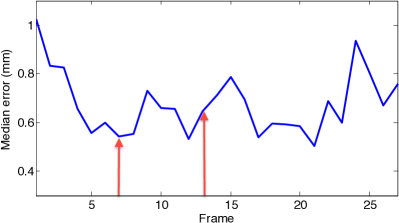
The results are shown in Fig. 13. As in the case of the sail of Fig. 6, we had a second sequence that we did not use for reconstruction purposes but used instead for validation purposes. To this end, we performed dense stereo reconstruction [38] and show in Fig. 14 the median distance between the resulting 3D point cloud and our monocular result. The undeformed ball diameter is 73.52 mm and the median distance hovers around 1% of that value except at the very beginning of the sequence when the ball is still undeformed but on the very left side of the frame. In fact, in those first few frames, it is the stereo algorithm that is slightly imprecise, presumably because the line of sight is more slanted. This indicates that it might not be perfectly accurate in the remaining frames either, thus contributing to some of the disagreement between the two algorithms.
5.3 Real Time Implementation
 |
 |
 |
 |
 |
| (a) | (b) | (c) | (d) | (e) |
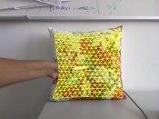
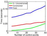
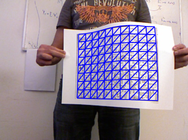
We have incorporated our approach to surface reconstruction into a real-time demonstrator that we showed at the CVPR’12 and ECCV’12 conferences. It was running at speeds of up to 10 frame-per-second on a MacBook Pro on images acquired by the computer’s webcam, such as those depicted by Fig. 15 that feature a planar sheet of paper and non-planar cushion such as those we used in our earlier experiments. The videos we supply as supplementary material demonstrate both the strengths and the limits of the approach: When there are enough correspondences, such as on the sheet of paper or in the center of the cushion, the 3D reconstruction is solid even when the deformations are severe. By contrast, on the edges of the cushion, we sometimes lose track because we cannot find enough correspondences anymore. To remedy this, a natural research direction would be to look into using additional image clues such as those provide by shading and contours, while preserving real-time performance.
Our C++ implementation relies on a feature-point detector to extract 500 interest points from the reference and 2000 ones from input images as maxima of the Laplacian and then uses the Ferns classifier [32] to match them. Additionally, since our algorithm can separate inlier correspondences from spurious ones, we track the former from images to images to increase our pool of potential correspondences, which turns out to be important when the surface deformations are large.
Given the correspondences in the first input image of a sequence, we use the outlier rejection scheme of Section 4.3 to eliminate the spurious one and obtain a 3D shape estimate. As long as the deforming surface is properly tracked, we can then simply estimate the 3D shape in subsequent frames by using the 3D shape estimate in a previous frame to initialize the constrained minimization of Eq. 12, without having to solve again the linear system of Eq. 10. However, if the system loses track, it can reinitialize itself by running the complete procedure again.
Real-time performance is made possible by the fact that the 3D shape estimation itself is fast enough to represent only a small fraction of the required computation, as shown in Fig. 15(e). A further increase in robustness and accuracy could be achieved by enforcing temporal consistency of the reconstructed shape from frame to frame [39, 40, 4].
We will release the real-time code on the lab’s website so that fellow researchers can try it for themselves.
6 Conclusion
We have presented a novel approach to parameterizing the vertex coordinates of a mesh as a linear combination of a subset of them. In addition to reducing the dimensionality of the monocular 3D shape recovery problem, it yields a rotation-invariant curvature-preserving regularization term that produces good results without training data or having to explicitly handle global rotations.
In our current implementation we applied constraints on every single edge of the mesh. In future work, we will explore other types of surface constraints in order to further decrease computational complexity without sacrificing accuracy. Another direction of research would be to take advantage of temporal consistency as has been done in many recent works [39, 40, 4] and of additional sources of shape information, such as shading and contours, to increase robustness and accuracy.
References
- [1] A. Bartoli, Y. Gérard, F. Chadebecq, and T. Collins, “On Template-Based Reconstruction from a Single View: Analytical Solutions and Proofs of Well-Posedness for Developable, Isometric and Conformal Surfaces,” in Conference on Computer Vision and Pattern Recognition, 2012.
- [2] M. Salzmann and P. Fua, Deformable Surface 3D Reconstruction from Monocular Images. Morgan-Claypool, 2010.
- [3] V. Blanz and T. Vetter, “A Morphable Model for the Synthesis of 3D Faces,” in ACM SIGGRAPH, August 1999, pp. 187–194.
- [4] M. Salzmann and P. Fua, “Linear Local Models for Monocular Reconstruction of Deformable Surfaces,” IEEE Transactions on Pattern Analysis and Machine Intelligence, vol. 33, no. 5, pp. 931–944, 2011.
- [5] N. Gumerov, A. Zandifar, R. Duraiswami, and L. Davis, “Structure of Applicable Surfaces from Single Views,” in European Conference on Computer Vision, May 2004.
- [6] J. Liang, D. Dementhon, and D. Doermann, “Flattening Curved Documents in Images,” in Conference on Computer Vision and Pattern Recognition, 2005, pp. 338–345.
- [7] M. Perriollat and A. Bartoli, “A Computational Model of Bounded Developable Surfaces with Application to Image-Based Three-Dimensional Reconstruction,” Computer Animation and Virtual Worlds, vol. 24, no. 5, 2013.
- [8] A. Ecker, A. Jepson, and K. Kutulakos, “Semidefinite Programming Heuristics for Surface Reconstruction Ambiguities,” in European Conference on Computer Vision, October 2008.
- [9] S. Shen, W. Shi, and Y. Liu, “Monocular 3D Tracking of Inextensible Deformable Surfaces Under L2-Norm,” in Asian Conference on Computer Vision, 2009.
- [10] F. Brunet, R. Hartley, A. Bartoli, N. Navab, and R. Malgouyres, “Monocular Template-Based Reconstruction of Smooth and Inextensible Surfaces,” in Asian Conference on Computer Vision, 2010.
- [11] R. White and D. Forsyth, “Combining Cues: Shape from Shading and Texture,” in Conference on Computer Vision and Pattern Recognition, 2006.
- [12] F. Moreno-noguer, M. Salzmann, V. Lepetit, and P. Fua, “Capturing 3D Stretchable Surfaces from Single Images in Closed Form,” in Conference on Computer Vision and Pattern Recognition, June 2009.
- [13] A. Malti, R. Hartley, A. Bartoli, and J.-H. Kim, “Monocular Template-Based 3D Reconstruction of Extensible Surfaces with Local Linear Elasticity,” in Conference on Computer Vision and Pattern Recognition, 2013.
- [14] F. Moreno-noguer, J. Porta, and P. Fua, “Exploring Ambiguities for Monocular Non-Rigid Shape Estimation,” in European Conference on Computer Vision, September 2010.
- [15] M. Perriollat, R. Hartley, and A. Bartoli, “Monocular Template-Based Reconstruction of Inextensible Surfaces,” International Journal of Computer Vision, vol. 95, 2011.
- [16] M. Salzmann, F. Moreno-noguer, V. Lepetit, and P. Fua, “Closed-Form Solution to Non-Rigid 3D Surface Registration,” in European Conference on Computer Vision, October 2008.
- [17] O. Sorkine, D. Cohen-Or, Y. Lipman, M. Alexa, C. Rössl, and H.-P. Seidel, “Laplacian Surface Editing,” in Symposium on Geometry Processing, 2004, pp. 175–184.
- [18] R. Sumner and J. Popovic, “Deformation Transfer for Triangle Meshes,” ACM Transactions on Graphics, pp. 399–405, 2004.
- [19] M. Botsch, R. Sumner, M. Pauly, and M. Gross, “Deformation Transfer for Detail-Preserving Surface Editing,” in Vision Modeling and Visualization, 2006, pp. 357–364.
- [20] J. Ostlund, A. Varol, D. Ngo, and P. Fua, “Laplacian Meshes for Monocular 3D Shape Recovery,” in European Conference on Computer Vision, 2012.
- [21] J. Fayad, L. Agapito, and A. Delbue, “Piecewise Quadratic Reconstruction of Non-Rigid Surfaces from Monocular Sequences,” in European Conference on Computer Vision, 2010.
- [22] R. Garg, A. Roussos, and L. Agapito, “Dense Variational Reconstruction of Non-Rigid Surfaces from Monocular Video,” in Conference on Computer Vision and Pattern Recognition, 2013.
- [23] M. Salzmann, R. Hartley, and P. Fua, “Convex Optimization for Deformable Surface 3D Tracking,” in International Conference on Computer Vision, October 2007.
- [24] P. Alcantarilla, P. Fernández, and A. Bartoli, “Deformable 3D Reconstruction with an Object Database,” in British Machine Vision Conference, 2012.
- [25] T. Cootes, G. Edwards, and C. Taylor, “Active Appearance Models,” in European Conference on Computer Vision, June 1998, pp. 484–498.
- [26] M. Dimitrijević, S. Ilić, and P. Fua, “Accurate Face Models from Uncalibrated and Ill-Lit Video Sequences,” in Conference on Computer Vision and Pattern Recognition, June 2004.
- [27] A. Delbue and A. Bartoli, “Multiview 3D Warps,” in International Conference on Computer Vision, 2011.
- [28] S. Ilić and P. Fua, “Using Dirichlet Free Form Deformation to Fit Deformable Models to Noisy 3D Data,” in European Conference on Computer Vision, May 2002.
- [29] A. Jacobson, I. Baran, J. Popovic, and O. Sorkine, “Bounded Biharmonic Weights for Real-Time Deformation,” in ACM SIGGRAPH, 2011.
- [30] P. Fua, A. Varol, R. Urtasun, and M. Salzmann, “Least-Squares Minimization Under Constraints,” EPFL, Tech. Rep., 2010.
- [31] D. Lowe, “Distinctive Image Features from Scale-Invariant Keypoints,” International Journal of Computer Vision, vol. 20, no. 2, 2004.
- [32] M. Ozuysal, M. Calonder, V. Lepetit, and P. Fua, “Fast Keypoint Recognition Using Random Ferns,” IEEE Transactions on Pattern Analysis and Machine Intelligence, vol. 32, no. 3, pp. 448–461, 2010.
- [33] Q.-H. Tran, T.-J. Chin, G. Carneiro, M. S. Brown, and D. Suter, “In defence of ransac for outlier rejection in deformable registration,” in European Conference on Computer Vision. Springer, 2012, pp. 274–287.
- [34] D. Pizarro and A. Bartoli, “Feature-Based Deformable Surface Detection with Self-Occlusion Reasoning,” International Journal of Computer Vision, March 2012.
- [35] J. Zhu and M. Lyu, “Progressive Finit Newton Approach to Real-Time Nonrigid Surface Detection,” in International Conference on Computer Vision, October 2007.
- [36] J. Pilet, V. Lepetit, and P. Fua, “Fast Non-Rigid Surface Detection, Registration and Realistic Augmentation,” International Journal of Computer Vision, vol. 76, no. 2, February 2008.
- [37] T. Collins and A. Bartoli, “Using isometry to classify correct/incorrect 3D-2D correspondences,” in European Conference on Computer Vision, 2014, pp. 325–340.
- [38] Y. Furukawa and J. Ponce, “Accurate, Dense, and Robust Multi-View Stereopsis,” IEEE Transactions on Pattern Analysis and Machine Intelligence, vol. 99, 2009.
- [39] L. Torresani, A. Hertzmann, and C. Bregler, “Nonrigid Structure-From-Motion: Estimating Shape and Motion with Hierarchical Priors,” IEEE Transactions on Pattern Analysis and Machine Intelligence, vol. 30, no. 5, pp. 878–892, 2008.
- [40] C. Russell, J. Fayad, and L. Agapito, “Energy Based Multiple Model Fitting for Non-Rigid Structure from Motion,” in Conference on Computer Vision and Pattern Recognition, 2011.
![[Uncaptioned image]](/html/1503.04643/assets/x141.png) |
Dat Tien Ngo is pursuing his Ph.D. at the computer vision laboratory, EPFL, under the supervision of Prof. Pascal Fua. He received his B.Sc. in Computer Science from Vietnam National University Hanoi with double title Ranked first in both entrance examination and graduation and his M.Sc. in Artificial Intelligence from VU University Amsterdam. His main research interests include deformable surface reconstruction, object tracking, augmented reality. |
![[Uncaptioned image]](/html/1503.04643/assets/x142.png) |
Jonas Östlund received his M.Sc. degree in computer science from Linköping University in 2010, along with the Tryggve Holm medal for outstanding academic achievements. From 2010 to 2013 he worked as a scientific assistant in the computer vision laboratory at EPFL, where his main research interest was monocular 3D deformable surface reconstruction with applications for sail shape modeling. Currently, he is co-founding the Lausanne-based startup Anemomind developing data mining algorithms for sailing applications. |
![[Uncaptioned image]](/html/1503.04643/assets/x143.png) |
Pascal Fua received an engineering degree from Ecole Polytechnique, Paris, in 1984 and the Ph.D. degree in Computer Science from the University of Orsay in 1989. He joined EPFL in 1996 where he is now a Professor in the School of Computer and Communication Science. Before that, he worked at SRI International and at INRIA Sophia-Antipolis as a Computer Scientist. His research interests include shape modeling and motion recovery from images, analysis of microscopy images, and Augmented Reality. He has (co)authored over 150 publications in refereed journals and conferences. He is an IEEE fellow and has been a PAMI associate editor. He often serves as program committee member, area chair, or program chair of major vision conferences. |
Appendix A Properties of the regularization term
Here we prove the claim made in Section 4.1.1 that when represents an affine transformed version of the reference mesh and that is invariant to rotations and translations.
The first equation in Eq. 13 applies for each of three spatial coordinates and can be rewritten in a matrix form as
| (28) |
It can be seen from Eq. 28 and the second equation in Eq. 13 that the three vectors of the components of the reference mesh and the vector of all 1s lie in the kernel of the matrix . It means our regularization term does not penalize affine transformation of the reference mesh. Hence, as long as represents an affine transformed version of the reference mesh.
Let be the new location of vertex under a rigid transformation of the mesh, where is the rotation matrix and is the translation vector. Since and , we have
Hence, when is a rigidly transformed version of . In other words, is invariant to rotations and translations.
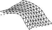
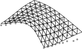
Appendix B Importance of Non-Linear Minimization
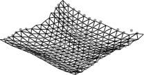
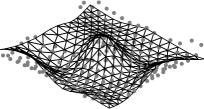
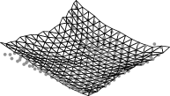
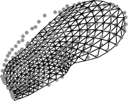
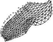
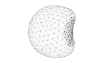
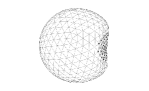
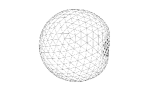
 |
 |
 |
 |
| (a) | (b) |
 |
 |
 |
 |
 |
 |
 |
 |
 |
 |
 |
 |
 |
 |
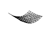 |
Fig. 16 illustrates the importance of the non-linear constrained minimization step of Eq. 12 that refines the result obtained by solving the linear least-squares problemof Eq. 10. In the left column we show the solution of the linear least-squares problem of Eq. 10. It projects correctly but, as evidenced by its distance to the ground-truth gray dots, its 3D shape is incorrect. By contrast, the surface obtained by solving the constrained optimization problem of Eq. 12 still reprojects correctly while also being metrically accurate. Fig. 17 depicts similar situations in other frames of the sequence.