Ordered Median Hub Location Problems with Capacity Constraints

Abstract

The Single Allocation Ordered Median Hub Location problem is a recent hub model introduced in [36] that provides a unifying analysis of a wide class of hub location models. In this paper, we deal with the capacitated version of this problem, presenting two formulations as well as some preprocessing phases for fixing variables. In addition, a strengthening of one of these formulations is also studied through the use of some families of valid inequalities. A battery of test problems with data taken from the AP library are solved where it is shown that the running times have been significantly reduced with the improvements presented in the paper.

1 Introduction

Network design problems are among the most interesting models in combinatorial optimization. In the last years researchers have devoted a lot of attention to a particular member within this family, namely the hub location problem, that combines network design and location aspects of supply chain models, see the surveys [1, 7, 9]. The main advantage of using hubs in distribution problems is that they allow to consolidate shipments in order to reduce transportation costs by applying economies of scale; which are naturally incorporated to the models through discount factors. Hub location problems have been studied from different perspectives giving rise to a number of papers considering different criteria to be optimized: the minimization of the overall transportation cost (sum) (see [10, 6, 20, 27, 29, 30, 31]), the minimization of the largest transportation cost or the coverage cost ([4, 8, 24, 25, 26, 34, 40, 41]), et cetera.

Apart from the choice of the optimization criterion, another crucial aspect in the literature on hub location, and in general on any location problem, is the assumption of capacity constraints. One can recognize that although this assumption implies more realistic models, the difficulty to solve them also increases in orders of magnitude with respect to their uncapacitated counterpart. In many cases new formulations are needed and a more specialized analysis is often required to solve even smaller sizes than those previously addressed for the uncapacitated versions of the problems. For this reason, capacitated versions of hub location problems have attracted the interest of locators in the last years, see [2, 5, 11, 13, 14, 15, 16, 20, 29]. In the same line, we also mention some other references related with congestion at hubs, as congestion acts as a limit on capacity, see [17, 18, 28].

An interesting version of hub location model is the Capacitated Hub Location Problem with Single Allocation (CSA-HLP), see [11, 13, 20]. In this context, single allocation means that incoming and outgoing flow of each site must be shipped via the same hub. In contrast to single allocation models, where binary variables are required in the allocation phase, multiple allocation allows different delivery patterns which in turns implies the use of continuous variables simplifying the problems. The CSA-HLP model incorporates capacity constraints on the incoming flow at the hubs coming from origin sites or even simpler, on the number of non-hub nodes assigned to each hub. The inclusion of capacity constraints make these models challenging from a theoretical point of view. Regarding its applicability we cite one example described in Ernst at al. [20] based on a postal delivery application, where a set of $n$ postal districts (corresponding to postcode districts represented by nodes) exchange daily mail. The mail between all the pairs of nodes must be routed via one or at most two mail consolidation centers (hubs). In order to meet time constraints, only a limited amount of mail could be sorted at each sorting center (mail is just sorted once, when it arrives to the first hub from origin sites). Hence, there are capacity restrictions on the incoming mail that must be sorted. The problem requires to choose the number and location of hubs, as well as to determine the distribution pattern of the mail.

The CSA-HLP has received less attention in the literature than its uncapacitated counterpart. Campbell [5] presented the first integer Mathematical Programming formulation for the Capacitated Hub Location Problem. This formulation was strenghthened by Skorin-Kapov et al. [39]. Ernst and Krishnamoorthy [20], proposed a new model involving three-index continuous variables and developed a solution approach based on Simulated Annealing where the bounds obtained are embedded in a branch-and-bound procedure devised for solving the problem optimally. Recently, Correia et al. [13] have shown that this formulation may be incomplete and an additional set of inequalities is proposed to assure the validity of the model in all situations. A new formulation using only two indices variables was proposed by Labbé et al. [27], where a polyhedral analysis and new valid inequalities were addressed. Although this formulation has only a quadratic number of variables, it has an exponential number of constraints, and to solve it the authors developed a branch-and-cut algorithm based on their polyhedral analysis. Contreras et al. [11] presented for the same problem a Lagrangean relaxation enhanced with reduction tests that allows the computation of tight upper and lower bounds for a large set of instances.

In two recent papers, [36, 37], a new model of hub location, namely the Single Allocation Ordered Median hub location problem (SA-OMHLP), has been introduced and analyzed. This problem can be seen as a powerful tool from a modeling point of view since it allows a common framework to represent many of the previously considered criteria in the literature of hub location. Moreover, this approach is a natural way to represent the differentiation of the roles played by the different parties (origins, hubs and destinations) in logistics networks [21, 22, 23, 32]. This model does not assume, in advance, any particular structure on the network ([11, 12]). Instead of that this structure is derived from the choice of the parameters defining the objective function. Apart from the above mentioned characteristics, ordered median objectives are also useful to obtain robust solutions in hub problems by applying $k$-centrum, trimmed-mean or anti-trimmed-mean criteria. It is worth mentioning that although it is called single allocation, its meaning slightly differs from the classical interpretation in hub location where each site is allocated to just one hub and all the incoming and outgoing flow to-from this site is shipped via the same link (the one joining this site and its allocated hub). In this model, single allocation means that all the outgoing flow is delivered through the same hub, but the incoming flow can come from different hubs. Actually, this is a mixed model and basically the same situation described above, about postal deliveries, naturally fits in this framework assuming that letters from the same origin should be sorted, with respect to their destinations, in the same place and from there they are delivered via their cheapest routes. Observe that in this scheme it is also natural that incoming flow in a final destination comes from different hubs.

The SA-OMHLP distinguishes among segmented origin-destination deliveries giving different scaling factors to the origin-hub, hub-hub and hub-destination links. The cost of each origin-first hub link is scaled by a factor that depends on the position of this cost in the ordered sequence of costs from each origin to its corresponding first hub [3, 32, 35]. Moreover, the overall interhub cost and hub-destination cost are multiplied by other economy of scale factors. The goal is to minimize the overall shipping cost under the above weighting scheme. The reader may note that the first type of scaling factors mentioned above adds a “sorting” problem to the underlying hub location model, making its formulation and solution much more challenging. This model and two different formulations were introduced in [35] while a specialized B&B&Cut algorithm was developed in [36, 38]. None of those formulations could handle capacities since the computation burden of the problems were highly demanding. Thus, the SA-OMHLP with capacity constraints, i.e. Capacitated Single Allocation Ordered Median hub location problem (CSA-OMHLP) is currently an open line of research for further analysis.

In this paper, we analyze in depth the CSA-OMHLP trying to obtain a better knowledge and alternative ways to solve it. Thus, the contributions of this paper are threefold. First, it combines for the first time three challenging elements in location analysis: hub facilities, capacities and ordered median objectives; proposing a promising IP formulation which remarkably reduces the number of decision variables. Second, this paper strengthens that formulation with variable fixing and some families of valid inequalities that have not been considered before. Finally, despite the difficulty of considering simultaneously capacitated models, hubs and ordering, the techniques proposed in this paper allow to solve instances of similar sizes to those already considered in the literature for simpler models (uncapacitated and multiple allocation [22]).

The paper is organized as follows: in Section 2 we will provide, first, a MIP formulation for the capacitated version of the problem extending the one in [36] and then another formulation in the spirit of [37] where the number of variables has been considerably reduced with respect to the previous one. Section 3 strengthens the latter formulations with variable fixing and several new families of valid inequalities. In Section 4, the effectiveness of the proposed methodology is shown with an extensive computational experience comparing the performance of the two formulations and the strengthening proposed along the paper. Finally, the paper ends with some conclusions.

2 Model and MIP formulations

The goal of this paper is to analyze the CSA-OMHLP. For this reason, we elaborate from the most promising formulations of the non-capacitated version of that problem, namely the so called radius (covering) formulations, see [36, 37]. In order to be self-contained and for the sake of readability, we include next a concise description of these formulations in their application to the capacitated problem.

Let $A=\{1,\ldots,n\}$ be a set of $n$ client sites, where each site is collecting or gathering some commodity that must be sent to the remaining ones. It is assumed, without loss of generality, that the set of candidate sites for establishing hubs is also A. Let $w_{jm}\geq 0$ be the amount of commodity to be supplied from the $j$-th to the $m$-th site for all $j,m\in A$, and let $W_{j}=\sum_{m\in A}w_{jm}$ be the total amount of commodity to be sent from the $j$-th site. Let $c_{jm}\geq 0$ denote the unit cost of sending commodity from site $j$ to site $m$ (not necessarily satisfying the triangular inequality). It is assumed free self-service, i.e., $c_{jj}=0$, $\forall j\in A$.

Let $p\leq n$ be the number of hubs to be located and let $b_{j}$ be the capacity of a hub located at site $j$, with $j\in A$. A solution for the problem is a set of sites $X\subseteq A$ with $|X|=p$ and enough capacity to cover the flow coming from the sites; plus a set of links connecting pairs (flow patterns) of sites $j$, $m$ for all $j,m\in A$. Moreover, it is assumed that the flow pattern between each pair of sites traverses at least one and no more than two hubs from $X$.

As it was mentioned in Section 1, the main advantage of using hubs is to reduce costs by applying economies of scale to consolidated flows in some part of the network. In this model the transportation cost is decoupled into the three differentiated possible links: origin site-first hub, hub-to-hub, and hubs-final destination. These transportation costs are scaled in a different way. The model weights origin site-first hub transportation costs by using parameters $\lambda=(\lambda_{1},\ldots,\lambda_{n})$, with $\lambda_{i}\geq 0\,\,\forall i\in A$, depending on their ordered rank values. This is, let $\hat{c}_{jk}$ be the cost of the overall flow sent from the origin site $j$ if it were delivered via the first hub $k$, i.e. $\hat{c}_{jk}:=c_{jk}W_{j},\,j,k\in A.$ Next, if $\hat{c}_{jk}$ were ranked in the $i$-th position among all these costs, then this term would be scaled by $\lambda_{i}$ in the objective function. For the two remaining links there is a compensation factor $0<\mu<1$ for the deliveries between hubs, and another one $0<\delta<1$, $\mu<\delta$, for the deliveries between hubs and final destination sites. These parameters may imply that, even in the case where the costs satisfy the triangle inequality, using a second hub results in a cheaper connection than going directly from the first hub to the final destination. Actually, it represents the application of the economy of scale by the consolidation of flow in the hubs.

In the following we present a first valid formulation of the CSA-OMHLP, based on covering variables (the reader is referred to [36, 37] for further details). Sorting the different delivery costs values $(\hat{c}_{jk})$ for $j,k\in A$, in increasing order, we get the ordered cost sequence:

$$\hat{c}_{(1)}:=0<\hat{c}_{(2)}<\cdots<\hat{c}_{(G)}:=\max\limits_{1\leq j,k\leq n}\{\hat{c}_{jk}\}.$$

where $G$ is the number of different elements of the above cost sequence. For convenience we consider $\hat{c}_{(0)}:=0$.

For $i\in A$ and $h=1,\ldots,G$, we define the following set of covering variables,

$$\bar{u}_{ih}:=\left\{\begin{array}[]{cl}1,&\mbox{if the $i$-th smallest allocation cost is at least $\hat{c}_{(h)}$,}\\[8.61108pt] 0,&\mbox{otherwise.}\end{array}\right.$$ (1)

Clearly, the $i$-th smallest allocation cost is equal to $\hat{c}_{(h)}$ if and only if $\bar{u}_{ih}=1$ and $\bar{u}_{i,h+1}=0$.
In addition, this formulation uses two more sets of variables:

$$x_{jk} = \begin{cases}1,&\mbox{if the commodity sent from origin site $j$ goes first to the hub $k$,}\\ 0,&\mbox{otherwise.}\end{cases}$$ (2)

$$s_{k\ell m} = \mbox{flow that goes through a first hub $k$ and a second hub $\ell$ with destination $m$},$$

with $j,k,\ell,m\in A.$ Since we assume that any origin is allocated to itself if it is a hub, the above definition implies that site $k$ is opened as a hub if the corresponding variable $x_{kk}$ takes the value 1.

The formulation of the model is:

$${(F_{\bar{u}})} \min \sum_{i\in A}\sum_{h=2}^{G}\lambda_{i}(\hat{c}_{(h)}-\hat{c}_{(h-1)})\bar{u}_{ih}+\sum_{k\in A}\sum_{\ell\in A}\sum_{m\in A}(\mu c_{k\ell}+\delta c_{\ell m})s_{k\ell m}$$ (3)

$$s.t. \sum_{k\in A}x_{jk}=1,\quad\forall j\in A$$ (14)

$$\sum_{j\in A}x_{jk}\leq nx_{kk},\quad\forall k\in A$$

$$\sum_{k\in A}x_{kk}=p$$

$$\sum_{\ell\in A}s_{k\ell m}=\sum_{j\in A}w_{jm}x_{jk},\quad\forall k,m\in A$$

$$s_{k\ell m}\leq\sum_{j\in A}w_{jm}(1-x_{mm})\quad\forall k,\ell,m\in A,\quad\ell\neq m$$

$$\sum_{\ell\in A}\sum_{m\in A}s_{k\ell m}\leq x_{kk}\sum_{j\in A}W_{j},\quad\forall k\in A$$

$$\sum_{k\in A}\sum_{m\in A}s_{k\ell m}\leq x_{\ell\ell}\sum_{j\in A}W_{j},\quad\forall\ell\in A$$

$${\sum_{j\in A}W_{j}x_{jk}\leq b_{k}x_{kk},\quad\forall k\in A}$$

$$\sum_{i\in A}\bar{u}_{ih}=\sum_{j\in A}\sum_{\stackrel{{\scriptstyle k=1}}{{\hat{c}_{jk}\geq\hat{c}_{(h)}}}}^{n}x_{jk},\quad\forall h=1,\ldots,G$$

$$\bar{u}_{ih}\geq\bar{u}_{i-1,h},\quad\forall i\in A\setminus\{1\},\>h=1,\ldots,G$$

$$\bar{u}_{ih},x_{jk}\in\{0,1\},s_{k\ell m}\geq 0,\quad\forall i,j,k,\ell,m\in A,\quad h=1,\ldots,G$$

The objective function (3) accounts for the weighted sum of the three components of the shipping cost, namely origin-first hub, hub-hub and hub-destination. The origin-hub costs are accounted after assigning the lambda parameters, i.e. $\sum\limits_{i\in A}\sum\limits_{h=2}^{G}\lambda_{i}\cdot(\hat{c}_{(h)}-\hat{c}_{(h-1)})\cdot\bar{u}_{ih}.$ In addition, the second and third blocks of delivery costs, i.e. the hub-hub and hub-destination cost, scaled with the $\mu$ and $\delta$ parameters respectively, can be stated as: $\sum_{k\in A}\sum_{\ell\in A}\sum_{m\in A}(\mu c_{k\ell}+\delta c_{\ell m})s_{k\ell m}.$

The constraints of the model are described in [36] with the only exception of (14), that is the capacity constraint on the hubs, in spite of that and for the sake of completeness we include below a brief description of them. Constraints (14) ensure that the flow from the origin site $j$ is associated with a unique first hub. Constraints (14) ensure that any origin only can be allocated to an open hub. Constraint (14) fixes the number of hubs to be located. Constraints (14) are flow conservation constraints, such that the flow that enters any hub $k$ with final destination $m$ is the same that the flow that leaves hub $k$ with destination $m$. Constraints (14) ensure that if the final destination site is a hub, then the flow goes at most through one additional hub. These constraints are redundant whenever the cost structure satisfies the triangular inequality, however they are useful in reducing solution times (see [36]). Constraints (14) and (14) establish again that the intermediate nodes in any origin-destination path should be open hubs. Constraints (14) establish the capacity constraints of the hubs. Observe that this family of constraints make redundant the family (14), but we have kept it because it reduces the computational times. Constraints (14) link sorting and covering variables. They state that the number of allocations with a cost at least $\hat{c}_{(h)}$ must be equal to the number of sites that support shipping costs to the first hub greater than or equal to $\hat{c}_{(h)}$. Finally, constraints (14) are a group of sorting conditions on the variables $\bar{u}_{ih}$.

The reader may note that this formulation is a natural extension for the capacitated version of the radius formulation already considered for the uncapacitated ordered median hub location problem in [36, 37]. However, although this formulation is enough to specify the CSA-OMHLP, we have found that for solving medium sized problems it produces very large MIP models, which are difficult to solve with standard MIP solvers (CPLEX, XPRESS; Gurobi…). Therefore, some alternatives should be investigated.

One way to improve the performance of the above formulation is to take advantage of some features of that model to reduce the number of variables. In this case, one can succeed reducing the number of $u$ variables. The logic of the above formulation can be further strengthen for important particular cases of the discrete ordered median hub location problem. In the following, we show a reformulation that is based on taking advantage of sequences of repetitions in the $\lambda$-vector. (See [33, 37, 38] for similar reformulations applied to other location problems.)

One can realize that for $\lambda$-vectors with sequences of repetitions –i.e. the center, $k$-centrum, trimmed means or median among others–, many variables used in formulation $F_{\bar{u}}$ are not necessary (since they are multiplied by zero in the objective function), and some others can be glued together (since they have the same coefficient in the objective function). Moreover, under the assumption of the free self-service, and that any origin is allocated to itself if it is a hub, we conclude that the $p$ smallest transportation costs from the origin to the first hubs are $0$, i.e. the first $p$ components of the $\lambda$-vector are multiplied by 0. Therefore, in order to simplify the problem one can disregard the $p$ first components of the $\lambda$-vector. Let $\tilde{\lambda}=(\tilde{\lambda}_{1},\ldots,\tilde{\lambda}_{n-p}):=(\lambda_{p+1},\ldots,\lambda_{n})$.

In order to give a formulation for the CSA-OMHLP taking advantage of these facts, we need to introduce some additional notation. Let $I$ be the number of blocks of consecutive equal non-null elements in $\tilde{\lambda}$ and define the vectors:

1. $\gamma=(\gamma_{1},\ldots,\gamma_{I})$, being $\gamma_{i}$, $i=1,\ldots,I$ the value of the elements in the $i$-th block of repeated elements in $\tilde{\lambda}$.

2. $\alpha=(\alpha_{1},\ldots,\alpha_{I},\alpha_{I+1})$, being $\alpha_{i}$ with $i=1,\ldots,I$, the number of zero entries between the $(i-1)$-th and $i$-th blocks of positive elements in $\tilde{\lambda}$ and $\alpha_{I+1}$ the number of zeros, if any, after the $I$-th block of non-null elements in $\tilde{\lambda}$. For notation purposes we define $\alpha_{0}=0$.

3. $\beta=(\beta_{1},\dots,\beta_{I})$, being $\beta_{i}$, $i=1,\ldots,I$ the number of elements in the $i$-th block of non-null elements in $\tilde{\lambda}$. For the sake of compactness, let $\beta_{0}=\beta_{I+1}=0$.

Next, let denote $\overline{\alpha}_{i}=\sum_{j=1}^{i}\alpha_{j}$, $\overline{\beta}_{i}=\sum_{j=1}^{i}\beta_{j}$ and recall that $W_{i}=\sum_{j\in A}w_{ij}$. Moreover, for all $i=1,\ldots,I$ and $h=1,\ldots,G$, let us define the following set of decision variables:

$$u_{ih} = \left\{\begin{array}[]{ll}1,&\mbox{if the }\displaystyle(p+\overline{\alpha}_{i}+\overline{\beta}_{i-1}+1)\mbox{-th assignment cost is at least }\hat{c}_{(h)},\\ 0,&\mbox{otherwise.}\end{array}\right.$$

$$v_{ih} = i$$ Number of assignments in the -th block between the positions

$$\displaystyle p+\overline{\alpha}_{i}+\overline{\beta}_{i-1}+1\mbox{ and }p+\overline{\alpha}_{i}+\overline{\beta}_{i}\mbox{ that are at least }\hat{c}_{(h)}.$$

With the above notation the formulation of CSA-OMHLP is:

$${(F_{uv})} \min \sum_{i=1}^{I}\sum_{h=2}^{G}\gamma_{i}(\hat{c}_{(h)}-\hat{c}_{(h-1)})v_{ih}+\sum_{k\in A}\sum_{\ell\in A}\sum_{m\in A}(\mu c_{k\ell}+\delta c_{\ell m})s_{k\ell m}$$ (17)

$$s.t. Constraints:(\ref{CCOV1})-(\ref{UUVC9}),$$

$$\sum_{i=1}^{I}\alpha_{i}u_{ih}+\sum_{i=1}^{I}v_{ih}+\alpha_{I+1}\geq\sum_{j\in A}\sum_{\stackrel{{\scriptstyle k\in A}}{{\hat{c}_{jk}\geq\hat{c}_{(h)}}}}x_{jk},\quad\forall h=2,\ldots,G$$

$$u_{ih}\geq u_{i-1,h},\quad\forall i=2,\ldots,I,\>h=1,\ldots,G$$ (22)

$$\beta_{i-1}u_{ih}\geq v_{i-1,h},\quad\forall i=2,\ldots,I,\>h=1,\ldots,G$$

$$v_{ih}\geq\beta_{i}u_{ih},\quad\forall i=1,\ldots,I,\quad h=1,\ldots,G$$

$$u_{ih}\in\{0,1\},v_{ih}\in\mathbb{Z}\cap[0,\beta_{i}],\quad\forall i=1\ldots,I,\quad h=1,\ldots,G$$

$$x_{jk}\in\{0,1\},s_{k\ell m}\geq 0,\quad\forall j,k,\ell,m\in A.$$

The objective function (17) is a reformulation of (3) substituting the $\bar{u}$ variables by the new $u$, $v$ variables and the vector $\gamma$, taking advantage of the $\lambda$ vector properties. Constraints (17) ensure that the number of sites that support a shipping cost to the first hub greater than or equal to $\hat{c}_{(h)}$ is either equal to the number of allocations with a cost at least $\hat{c}_{(h)}$ whenever $v_{Ih}>0$ or less than or equal to $\alpha_{I+1}$ otherwise. Constraints (22) are sorting constraints on the variables $u$ similar to constraints (14), and constraints (22)-(22) provide upper and lower bounds on the variables $v$ depending on the values of variables $u$.

The main difference between $F_{\bar{u}}$ and $F_{uv}$ is that all $\bar{u}_{ih}$ variables associated with blocks of zero $\lambda$-values are removed, and those associated with each block of non-null $\lambda$ values are replaced by $2\times G$ variables. Therefore, overall we reduce the number of variables by $(n-2I)\times G$.

Note that in Formulation $F_{\bar{u}}$, the family of constraints that links covering variables (variables $\bar{u}$) and the allocation variables (variables $x$), i.e. (14), is given with equalities. This fact implies that the actual dimension of the feasible region in the space of $\bar{u}$ and $x$ variables is smaller than the one that we were currently working on. This is exploited in the new formulation. Indeed, we reduce the number of variables used in the sorting phase replacing $\bar{u}$ by $u$ and $v$. Therefore, the dimension of the feasible region in the space of $u$, $v$, $x$ variables has smaller dimension. In addition, the constraints that link sorting and design variables, namely (17), are given as inequalities. This new representation, although valid for the problem, induces some loss of information in that it does not allow us to take full control of the exact number of allocations at some specific cost. This does not affect the resolution process but influences the derivation of valid inequalities.

Finally, for those cases where $\beta_{i}=1$ we observe that $v_{ih}=u_{ih}$. This set of constraints whenever valid, was added to reinforce the formulation.

Example 2.1

To illustrate how the $F_{uv}$ versus $F_{\bar{u}}$ formulations work, we consider the following data. Let $A=\{1,\dots,6\}$ be a set of sites and assume that we are interested in locating $p=2$ hubs. Let the cost and flow matrices be as follows:

$$C=\left(\begin{array}[]{cccccccccccc}0&14&15&16&15&9\\ 5&0&7&2&19&16\\ 16&5&0&7&1&19\\ 12&1&10&0&13&1\\ 1&9&9&15&0&2\\ 8&10&16&8&4&0\\ \end{array}\right),\;W=\left(\begin{array}[]{cccccccccccc}0&15&2&8&11&2\\ 19&0&1&16&20&7\\ 3&9&0&3&11&16\\ 7&2&5&0&14&5\\ 15&4&20&4&0&1\\ 12&4&7&11&18&0\\ \end{array}\right).\;$$

Therefore, $\hat{c}_{(\cdot)}$, the sorted vector of $\hat{c}$, is in our case
$\hat{c}_{(\cdot)}=[0,33,42,44,88,126,208,210,294,315,330,342,396,416,429,441,520,532,570,608,660,\\ 672,798,832,1008,{1197}].$ Hence, $G=26$. Let $\lambda=(0,1,0,0,1,1)$, $\mu=0.7$, $\delta=0.9$, and the capacity constraints vector $b=(119,119,113,145,149,140)$. The optimal solution opens hubs $4$ and $6$. The allocation of origin sites to first hub is given by the following values of the variables $x$ (see Figure 1):

$$x_{16}=x_{24}=x_{34}=x_{44}=x_{56}=x_{66}=1.$$

Analogously, the allocation of first hubs to final destinations are given by the values of the non null variables $s$. Thus, the flows considering as first hubs $4$ and $6$ are (see Figure 1 for a graphical representation of the delivery paths):

$$s_{442}=11,\>s_{443}=6,\>s_{444}=19,\>s_{461}=29,\>s_{465}=45,\>s_{466}=28;$$

$$s_{642}=23,\>s_{644}=23,\>s_{661}=27,\>s_{663}=29,\>s_{665}=29,\>s_{666}=3.$$

Figure 1: Illustration of Example 2.1. Left figure represents the allocations of sites to their corresponding first hubs. Right figure represents the flow pattern to the final destinations from the first hubs: 4 (dashed lines) and 6 (grey lines).

Moreover, the covering variables $\bar{u}_{ih}$ are given below. Due to their structure, we only report for each $i$ the last one and first zero occurrences since they characterize the remaining values.

$$\begin{array}[]{lll}i=1\mapsto\bar{u}_{11}=1,\bar{u}_{12}=0&i=2\mapsto\bar{u}_{21}=1,\bar{u}_{22}=0&i=3\mapsto\bar{u}_{35}=1,\bar{u}_{36}=0\\ i=4\mapsto\bar{u}_{46}=1,\bar{u}_{47}=0&i=5\mapsto\bar{u}_{59}=1,\bar{u}_{5,10}=0&i=6\mapsto\bar{u}_{6,12}=1,\bar{u}_{6,13}=0.\\ \end{array}$$

The first two assignments are done at a cost $c_{(1)}=0$, corresponding to the two hubs ($p=2$). The next assignment has been done at a cost $c_{(5)}=88$, since $\bar{u}_{35}=1$ and $\bar{u}_{36}=0$, and so on. The rest of assignments costs are then $c_{(6)}=126$, $c_{(9)}=294$ and $c_{(12)}=342$.

Hence, the overall cost of this solution is

$$\sum_{i\in A}\sum_{h=2}^{G}\lambda_{i}(\hat{c}_{(h)}-\hat{c}_{(h-1)})\bar{u}_{ih}+\sum_{k\in A}\sum_{\ell\in A}\sum_{m\in A}(\mu c_{k\ell}+\delta c_{\ell m})s_{k\ell m}=636+1500.8=2136.8.$$

In addition, to illustrate how the formulation $F_{uv}$ is related with $F_{\bar{u}}$, we also include the solution of the covering variables ${u}_{ih}$ and ${v}_{ih}$:

$$\begin{array}[]{l}I=1\mapsto{u}_{16}=1,u_{17}=0\\ I=1\mapsto{v}_{11}=\ldots=v_{19}=2;\>{v}_{1,10}=\ldots=v_{1,12}=1;\>v_{1,13}=0\end{array}$$

$$\bar{u}_{i,h}=\begin{array}[]{c}\\ {{}_{1}}\\ {{}_{2}}\\ {{}_{3}}\\ {{}_{4}}\\ {{}_{5}}\\ {{}_{6}}\\ \end{array}\begin{array}[]{c}{\tiny\begin{array}[]{cccccccccc}c_{(1)}&c_{(2)}&c_{(3)}&c_{(4)}&c_{(5)}&c_{(6)}&\ldots&c_{(24)}&c_{(25)}&c_{(26)}\end{array}}\\ \left(\begin{array}[]{cccccccccc}\hskip 4.26773pt1&\hskip 4.26773pt0&\hskip 4.26773pt0&\hskip 4.26773pt0&\hskip 4.26773pt0&\hskip 4.26773pt0&\hskip 4.26773pt\ldots&\hskip 4.26773pt0&\hskip 4.26773pt0&\hskip 4.26773pt0\\ 1&0&0&0&0&0&\ldots&0&0&0\\ 1&1&1&1&1&0&\ldots&0&0&0\\ 1&1&1&1&1&1&\ldots&0&0&0\\ 1&1&1&1&1&1&\ldots&0&0&0\\ 1&1&1&1&1&1&\ldots&0&0&0\\ \end{array}\right)\\ \end{array}\Rightarrow\lambda=\begin{array}[]{c}\begin{array}[]{lrl}&&\end{array}\\ \left(\begin{array}[]{c}0\\ 1\\ 0\\ 0\\ 1\\ 1\end{array}\right)\end{array}\begin{array}[]{c}\begin{array}[]{lrl}&&\end{array}\\ \begin{array}[]{ll}\left\}\begin{array}[]{rl}{\it}\hfil&\\ {\it}\hfil\end{array}\right.&p\\ \left\}\begin{array}[]{rl}{}\hfil&\\ {}\hfil\end{array}\right.&\alpha_{1}\\ \left\}\begin{array}[]{rl}{}\hfil&\\ {}\hfil\end{array}\right.&\beta_{1}\left\}\begin{array}[]{r}v_{1}\end{array}\right.\end{array}\end{array}\begin{array}[]{c}\begin{array}[]{lrl}&&\end{array}\\ \begin{array}[]{ll}&\\ &\\ &\\ &\\ \longrightarrow\longrightarrow u_{1}&\\ &\\ \end{array}\end{array}$$

Figure 2: Variables and lambda vector of Example 2.1

Note that we have only one block of repeated non-null elements of the $\tilde{\lambda}$-vector, so $I=1$. (See the right part of Figure 2.) The number of zero entries between two blocks is $\alpha_{1}=2$, and the number of elements in the $1$-st block of non-null elements is $\beta_{1}=2$. Furthermore, $\gamma_{1}=1$ is the repeated value in the $1$-st block.

$$\begin{array}[]{c}{\tiny\begin{array}[]{p{.5cm}p{.5cm}p{.5cm}p{.5cm}p{.5cm}p{.5cm}p{.5cm}p{.5cm}p{.5cm}p{.5cm}p{.5cm}p{.5cm}p{.5cm}p{.5cm}p{.5cm}p{.5cm}p{.5cm}p{.5cm}}&$c_{(1)}$&$c_{(2)}$&$c_{(3)}$&$\ldots$&$c_{(9)}$&$c_{(10)}$&$c_{(11)}$&$c_{(12)}$&$c_{(13)}$&$c_{(14)}$&$c_{(15)}$&$c_{(16)}$&$c_{(17)}$&$\ldots$&$c_{(25)}$&$c_{(26)}$\end{array}}\\ {u}_{1,h}=(\begin{array}[]{p{.5cm}p{.5cm}p{.5cm}p{.5cm}p{.5cm}p{.5cm}p{.5cm}p{.5cm}p{.5cm}p{.5cm}p{.5cm}p{.5cm}p{.5cm}p{.5cm}p{.5cm}p{.5cm}p{.3cm}}$1$&$1$&$1$&\ldots&$1$&$1$&$1$&$1$&$1$&$1$&$1$&$1$&$0$&\ldots&$0$&$0$\end{array})\\ {v}_{1,h}=(\begin{array}[]{p{.5cm}p{.5cm}p{.5cm}p{.5cm}p{.5cm}p{.5cm}p{.5cm}p{.5cm}p{.5cm}p{.5cm}p{.5cm}p{.5cm}p{.5cm}p{.5cm}p{.5cm}p{.5cm}p{.3cm}}$2$&$2$&$2$&\ldots&$2$&$1$&$1$&$1$&$0$&$0$&$0$&$0$&$0$&\ldots&$0$&$0$\end{array})\\ \end{array}$$

The variable ${u}_{1,h}$ points out to the row $p+\alpha_{1}+1=5$ of the original variable $\bar{u}_{i,h}$. Whereas the variable ${v}_{1,h}$ accounts for the number of assignments between the positions $p+\alpha_{1}+1=5$ and $p+\alpha_{1}+\beta_{1}=6$ of $\bar{u}_{i,h}$ that are at least $\hat{c}_{(h)}$. (See Figure 2.)

From $\bar{u}_{i,h}$, we know that the $5$-th assignment cost is $\hat{c}_{(9)}$ and the $6$-th assignment cost is $\hat{c}_{(12)}$. For this reason ${v}_{1,h}$ is equal to $2$ up to column $9$, this is the number of assignment costs greater than $\hat{c}_{(9)}$. Being this number equal to 1 from $h=10$ to $h=12$, and zero for the remaining columns.

Applying this formulation, the overall reduction in the number of variables is $(n-2I)\times G=104$. The rest of variables $x$ and $s$ remain the same, and again the overall cost of this solution is

$$\sum_{i=1}^{I}\sum_{h=2}^{G}\gamma_{i}(\hat{c}_{(h)}-\hat{c}_{(h-1)})v_{ih}+\sum_{k\in A}\sum_{\ell\in A}\sum_{m\in A}(\mu c_{k\ell}+\delta c_{\ell m})s_{k\ell m}={636+1500.8=2136.8}.$$

3 Strengthening the formulation

3.1 Variable fixing

Next, we describe some preprocessing procedures that we have applied to reduce further the size of formulation $F_{uv}$. We present a number of variable fixing possibilities for the set of variables $u$ and $v$ which are useful in the overall solution process. The variable fixing procedures developed in this section are based on ideas used in [36, 37] and taking advantage of the capacity constraints. Indeed, we are adding the reinforced effective capacity constraints, as well as some surrogated version of constraints (3.1.1) since in this aggregated form they give better running times. The preprocessing phase developed in this paper also provides new upper and lower bounds on the $v$ variables. The percentage of variable reduction obtained by these procedures can be found in Tables 1 and 2 (column named as ’Fixed’).

Before describing these procedures for fixing variables, the following simple arguments allows us to fix some variables:

1. First, $c_{jj}=0$ $\forall j\in A$, i.e., $\hat{c}_{(1)}=0$. Moreover, every origin where it has been located a hub will be allocated to itself as a first hub.

2. Second, $\hat{c}_{jk}\neq 0$ if and only if $j\neq k$, i.e., any non-hub origin is allocated to a first hub at a cost of at least $\hat{c}_{(2)}$.

Therefore, since in this formulation the first $p$-allocations are considered only implicitly, we can fix $u_{i1}=1$, $v_{i1}=\beta_{i}$ as well as $u_{i2}=1$, $v_{i2}=\beta_{i}$, $\forall i=1,\ldots,I.$

3.1.1 Preprocessing Phase 1: Fixing variables to the upper bounds for the formulation with covering variables strengthen with capacity constraints.

Due to the definition of the variables in formulation $F_{uv}$, one can expect that $u_{ih}=1$ whenever $i$ is large and $h$ is small to medium size because this would mean that the $(p+\overline{\alpha}_{i}+\overline{\beta}_{i-1}+1)$-th sorted allocation cost would not have been done at cost less than $\hat{c}_{(h)}$. The reader should observe that an analogous strategy applies to the variables $v$ since their interpretation is similar, but in this case the values of $v_{ih}$ would be fixed to $\beta_{i}$. For the cases where it is not possible to fix the corresponding $v$-variable, it could be still possible to establish some lower bounds as we will see later.

Next, to fix variables $u_{ih}$ and $v_{ih}$ for $i=1,\ldots,I$, $h=1,\ldots,G$, we deal with an auxiliary problem that maximizes the number of variables that may assume zero values, satisfying $\hat{c}_{jk}\leq\hat{c}_{(h-1)}$ and the capacity constraints. For any $h=1,\ldots,G$ and $j,k\in A$ such that $\hat{c}_{jk}\leq\hat{c}_{(h-1)}$ let

$$z_{jk}^{h}=\begin{cases}1,&\mbox{if origin site $j$ is assigned to hub $k$}\\ 0,&\mbox{otherwise.}\end{cases}$$ (23)

To avoid possible misunderstanding in the cases where variables $z_{jk}^{h}$ are not defined, i.e. when $\hat{c}_{jk}>\hat{c}_{(h-1)}$, we can assume that $z_{jk}^{h}:=0$.

For a given $h$, we introduce the effective capacity of a hub $k$ at a cost at most $\hat{c}_{(h-1)}$ as,

$${b_{k}^{h-1}}:=\min\left\{b_{k},\sum_{\stackrel{{\scriptstyle s\in A}}{{\hat{c}_{sk}\leq\hat{c}_{(h-1)}}}}W_{s}\right\}.$$ (24)

Indeed, the capacity of a hub $k$ is always lower than or equal to $b_{k}$. In addition, if we restrict ourselves to the nodes served at a cost of at most $\hat{c}_{(h-1)}$, then the actual capacity to cover this set should be lower than $\sum_{s\in A:\hat{c}_{sk}\leq\hat{c}_{(h-1)}}W_{s}$, and this gives us the expression of ${b_{k}^{h-1}}$.

The optimal value $P_{1}(h)$ of the following problem fixes the maximal number of allocations that may be feasible at a cost of at most $\hat{c}_{(h-1)}$.

$$P_{1}(h):= \max {\sum_{\stackrel{{\scriptstyle j,k\in A:}}{{\hat{c}_{jk}\leq\hat{c}_{(h-1)}}}}}z^{h}_{jk}$$

$$s.t. {\sum_{{k\in A:}{\hat{c}_{jk}\leq\hat{c}_{(h-1)}}}}z^{h}_{jk}\leq 1,\quad\forall j\in A,$$

$${\sum_{{j\in A:}{\hat{c}_{jk}\leq\hat{c}_{(h-1)}}}}z^{h}_{jk}\leq ny_{k},\quad\forall k\in A$$

$$\sum_{k\in A}y_{k}\leq p$$

$${\sum_{j\in A:\hat{c}_{jk}\leq\hat{c}_{(h-1)}}}W_{j}z^{h}_{jk}\leq{b_{k}^{h-1}}y_{k},\quad\forall k\in A$$

$$z^{h}_{jk},y_{k}\in\{0,1\},\quad\forall j,k\in A,\;\forall h=1,\ldots,G.$$

Then, depending on the value $P_{1}(h)$ we can fix some variables to their upper bounds. Let us denote by $i_{1}(h)\in\{1,\ldots,I\}$ the index such that

$$p+\overline{\alpha}_{i_{1}(h)-1}+\overline{\beta}_{i_{1}(h)-1}<P_{1}(h)\leq p+\overline{\alpha}_{i_{1}(h)}+\overline{\beta}_{i_{1}(h)}.$$

$$\left\{\begin{array}[]{ll}u_{ih}=1,v_{ih}=\beta_{i},\;i=i_{1}(h),\ldots,I,&\mbox{if }\displaystyle P_{1}(h)\leq p+\overline{\alpha}_{i_{1}(h)}+\overline{\beta}_{i_{1}(h)-1}\\ \left\{\begin{array}[]{l}\displaystyle v_{i_{1}(h),h}\geq p+\overline{\alpha}_{i_{1}(h)}+\overline{\beta}_{i_{1}(h)}-P_{1}(h),\\ u_{ih}=1,\quad v_{ih}=\beta_{i},\;i=i_{1}(h)+1,\ldots,I,\end{array}\right\}&\mbox{otherwise.}\end{array}\right.$$

3.1.2 Preprocessing Phase 2: Fixing variables to their lower bounds

Following similar argument to the previous subsection, one can expect that many variables $u$ and $v$ in the top-right hand corner of the matrices of variables $u$ and $v$ , respectively, will take value 0 in the optimal solution. Indeed, $u_{ih}=0$ means that the $(p+\overline{\alpha}_{i}+\overline{\beta}_{i-1}+1)$-th sorted allocation cost is less than $\hat{c}_{(h)}$ which is very likely to be true if $h$ is sufficiently large and $i$ is small. Note that an analogous strategy, applies to the variables $v$ since their interpretation is similar. For the cases where it is not possible to fix the corresponding $v$-variable it could be still possible to establish some upper bounds.

For any $h=2,\ldots,G$, $j,k\in A$ such that $\hat{c}_{jk}\geq\hat{c}_{(h-1)}$ let define variables $z_{jk}^{h}$ as (23). To avoid possible misunderstanding in the cases where variables $z_{jk}^{k}$ are not defined, i.e. when ${\hat{c}_{jk}<\hat{c}_{(h-1)}}$, we can assume that ${z_{jk}^{h}}:=0$. Using these variables, the formulation of the problem that maximizes the number of non-fixed allocations at a cost at most $\hat{c}_{(h-1)}$ is:

$$P_{2}(h):= \max {\sum_{\stackrel{{\scriptstyle j,k\in A:}}{{\hat{c}_{jk}\geq\hat{c}_{(h-1)}}}}}{z_{jk}^{h}}$$

$$s.t. {\sum_{{k\in A:}{\hat{c}_{jk}\geq\hat{c}_{(h-1)}}}}{z_{jk}^{h}}\leq 1,\quad\forall j\in A$$

$${\sum_{{j\in A:}{\hat{c}_{jk}\geq\hat{c}_{(h-1)}}}}{z_{jk}^{h}}\leq ny_{k},\quad\forall j,k\in A$$

$$\sum_{k\in A}y_{k}\leq p,$$

$${z_{jk}^{h}},y_{k}\in\{0,1\},\quad\forall j,k\in A,\;\forall h=1,\ldots,G.$$

Note that the value $P_{2}(h)$ implies that there are no feasible solutions of the original problem with less than $n-P_{2}(h)$ allocations fixed at a cost at most $\hat{c}_{(h)}$.

Let $1\leq i_{2}(h)\leq I$ be the index such that

$$p+\overline{\alpha}_{i_{2}(h)-1}+\overline{\beta}_{i_{2}(h)-1}<n-P_{2}(h)\leq p+\overline{\alpha}_{i_{2}(h)}+\overline{\beta}_{i_{2}(h)}.$$

Thus, in any feasible solution of the problem we have that:

$$\left\{\begin{array}[]{ll}u_{ih}=0,v_{ih}=0,\>i=1,\ldots,i_{2}(h)-1,&\mbox{if }\displaystyle n-P_{2}(h)\leq p+\overline{\alpha}_{i_{2}(h)}+\overline{\beta}_{i_{2}(h)-1}\\ \left\{\begin{array}[]{l}\displaystyle u_{i_{2}(h),h}=0,\quad v_{i_{2}(h),h}\leq p+\overline{\alpha}_{i_{2}(h)}+\overline{\beta}_{i_{2}(h)}-(n-P_{2}(h)),\\ u_{ih}=0,\quad v_{ih}=0,\quad i=1,\dots,i_{2}(h)-1,\end{array}\right\}&\mbox{otherwise.}\end{array}\right.$$

Note that whenever $n-P_{2}(h)=p$ then there is nothing to fix and therefore no variables are set to zero in column $h$.

3.2 Valid Inequalities

In order to strengthen formulation $F_{uv}$ we have studied several families of valid inequalities. In fact, taking advantage of previous experience on the non-capacitated version of the problem we have borrowed a first family of valid inequalities that are very simple and that have proven to be effective in different ordered median problems with covering variables [36, 37]. This family is

$$u_{ih}\geq u_{i,h+1}, i=1,\ldots,I,\;h=1,\ldots,G-1,$$ (27)

$$v_{ih}\geq v_{i,h+1}, i=1,\ldots,I,\;h=1,\ldots,G-1.$$ (28)

Since, these families are straightforward consequence of the definition of variables $u$ and $v$ they have been included in the original formulation.

In the following, we describe several alternative families of valid inequalities: three sets of inequalities, (29),(30)-(33), and (• ‣ 3.2.2)-(• ‣ 3.2.2), based on the combination of ordering and capacity requirements and two more sets, (38) and (39)-(40), that do not use capacities.

3.2.1 First family of valid inequalities: Valid inequalities based on capacity I

We can add to this model several families of valid inequalities based on capacity issues that help in solving the problem by reducing the gap of the linear relaxation and the CPU time to explore the branch and bound search tree.

Observe that the capacity of the set of hubs that may be used to assign origins in $A$ at a cost at most $\hat{c}_{(h-1)}$, is given by

$$\sum_{k\in A}{b_{k}^{h-1}}x_{kk}$$

where $\displaystyle{b_{k}^{h-1}}$ is the effective capacity at a cost at most $\hat{c}_{(h-1)}$, defined by (24). Recall that, although the capacity of a hub $k$ is always lower than or equal to $b_{k}$, when we restrict to the nodes served at a cost of at most $\hat{c}_{(h-1)}$, then the actual capacity to cover this set should be lower than $b_{k}^{h-1}$. Making use of the above observation, we can add the following family of constrains as valid inequalities

$$\sum_{\stackrel{{\scriptstyle j\in A}}{{\hat{c}_{jk}\leq\hat{c}_{(h-1)}}}}W_{j}x_{jk}\leq{b_{k}^{h-1}}x_{kk}\quad\forall h=2,\ldots,G,k\in A$$ (29)

which enforces that all the flow sent from origin-hubs at a cost at most $\hat{c}_{(h-1)}$ cannot exceed the effective capacity at that cost. Observe that in the case where $b_{k}^{h-1}$ takes the value $b_{k}$ (11) dominates (29), but in the case where $b_{k}^{h-1}=\sum_{{s\in A:}{\hat{c}_{sk}\leq\hat{c}_{(h-1)}}}W_{s}$, (29) becomes $\sum_{{j\in A:}{\hat{c}_{jk}\leq\hat{c}_{(h-1)}}}W_{j}x_{jk}\leq\sum_{{j\in A:}{\hat{c}_{jk}\leq\hat{c}_{(h-1)}}}W_{j}x_{kk}$. Observe that this last valid inequality is an alternative surrogation, with capacity coefficients, of constraints $x_{jk}\leq x_{kk}$ that although valid do not appear in the model because of its large cardinality. This new form of aggregation has provided good results in the computational experiments.

3.2.2 Second family of valid inequalities: Valid inequalities based on capacity II

This section introduces another family of valid inequalities based on capacity issues that help in solving the problem. In order to present these new valid inequalities based on capacity requirements we introduce some new notation. Assume without loss of generality that $W_{i}\leq W_{i+1}$ for $i\in A\setminus\{n\}$ and let $\overline{W}_{j}=\sum_{r=1}^{j}W_{r}$ and $S_{k}:=\{i\in A:i\leq k\}$ for $k\in A$ be a given set of origin sites.

In case that the effective capacity at a cost at most $\hat{c}_{(h-1)}$ is not sufficient to cover the demand of $S_{k}$, i.e. $\displaystyle\sum^{n}_{j=1}\Big{(}b_{j}^{h-1}-W_{j}\Big{)}x_{jj}$ is less than $\sum_{s=1}^{k}W_{s}(1-x_{ss})$, then at most $k-1$ origins of $S_{k}$ can be allocated at a cost lower than or equal to $\hat{c}_{(h-1)}$. This argument can be applied for each $h$ to the corresponding $\hat{c}_{(h-1)}$ value. Moreover, we have chosen this particular structure of $S_{k}$ consisting of the $k$ origins (nodes) with the $k$-smallest flows, because given a fixed amount of flow, the maximal cardinality set of origins, such that the overall flow originated in this set is lower than or equal to this amount, is provided by a set $S_{k}$ for some $k\in A$. Therefore, since we are dealing with the worst cases, it allows us to fix some variables $u$ and $v$ through the following valid inequalities. For each $h=2,\ldots,G$ we obtain the following:

• If $\overline{\alpha}_{i-1}+\overline{\beta}_{i-1}<k\leq\overline{\alpha}_{i}+\overline{\beta}_{i-1}+1$, for some $i\in\{1,\ldots,I\}$, namely if the index of the last element, $k$, that defines $S_{k}$ lies in the $i$-th block of null elements in the $\tilde{\lambda}$ vector, then

  $$\overline{W}_{k}u_{ih}+\sum_{j\in A}\Big{(}b_{j}^{h-1}-W_{j}\Big{)}x_{jj}\geq\sum_{s=1}^{k}W_{s}(1-x_{ss}).$$ (30)

  Observe that the above inequality amounts to a disjunctive condition: either the effective capacity at a cost at most $\hat{c}_{(h-1)}$ is enough to cover the demand of the $k$ smallest flows from origin sites or the $i$-th sorted cost allocation must be assigned at a cost at least $c_{(h)}$.

• If $\overline{\alpha}_{i}+\overline{\beta}_{i-1}+1<k\leq\overline{\alpha}_{i}+\overline{\beta}_{i}$, and namely if the index of the last element, $k$, that defines $S_{k}$ lies in the $i$-th block of non-null elements, then

  $$\overline{W}_{k}v_{ih}+\sum_{j\in A}\Big{(}b_{j}^{h-1}-W_{j}\Big{)}x_{jj}\geq\sum_{s=1}^{k}W_{s}(1-x_{ss}).$$ (31)

  In this case, the inequality is similar to the previous one but written in terms of the variables $v$ that allow to control the capacity whenever $k$ falls within a block of non-null elements in the $\tilde{\lambda}$ vector.

Remark 3.1

Recall that if $k>P_{1}(h)-p$, variables $u_{ih}$ and $v_{ih}$ have been already fixed by the Preprocessing Phase 1, and for the above inequality to be effective $k\leq P_{1}(h)-p$, or equivalently, $i\leq i_{1}(h)$ .

Based on the same arguments we can add a larger family of valid inequalities built on arbitrary sets of origin sites. Let $S$ be a set of origin sites, and suppose that $A_{S}=\sum_{s\in S}W_{s}$ satisfies $\overline{W}_{k}\leq A_{S}<\overline{W}_{k+1}$ ,

• If $\overline{\alpha}_{i-1}+\overline{\beta}_{i-1}<k\leq\overline{\alpha}_{i}+\overline{\beta}_{i-1}+1$, for some $i\in\{1,\ldots,I\}$, and $k\leq P_{1}(h)-p$ then

  $$A_{S}u_{ih}+\sum_{j\in A}\Big{(}b_{j}^{h-1}-W_{j}\Big{)}x_{jj}\geq\sum_{s=1}^{k}W_{s}(1-x_{ss}).$$ (32)

• If $\overline{\alpha}_{i}+\overline{\beta}_{i-1}+1<k\leq\overline{\alpha}_{i}+\overline{\beta}_{i}$, and $k\leq P_{1}(h)-p$ then

  $$A_{S}v_{ih}+\sum_{j\in A}\Big{(}b_{j}^{h-1}-W_{j}\Big{)}x_{jj}\geq\sum_{s=1}^{k}W_{s}(1-x_{ss}).$$ (33)

Now, assuming a more general case and for an improvement of the above inequalities (30) and (31), for a given $h\in\{2,\ldots,G\}$, and $k\leq P_{1}(h)-p$, $k\in\{1,\ldots,\overline{\alpha}_{I+1}+\overline{\beta}_{I})\}$, let

$$M_{s}:=\min_{j(\neq s)\in A}\hat{c}_{js}.$$

$M_{s}$ is the minimum allocation cost to $s$ as an open hub. In other words, no allocation to hub $s$ is possible at a cost less than $M_{s}$, except in case $s$ were a hub itself. We shall call this value the empty radius of $s$.

Define $s(h-1,k)$ to be the index of the sorted sequence of elements $W_{s}$ such that there are exactly $k$ elements $W_{s}$ with $s\leq s(h-1,k)$ and $M_{s}\leq\hat{c}_{(h-1)}$, namely $s(h-1,k)$, is the index such that

$$|\{s\>:\>s\leq s(h-1,k);\>M_{s}\leq\hat{c}_{(h-1)}\}|=k.$$

Then it holds that,

• If $\overline{\alpha}_{i-1}+\overline{\beta}_{i-1}<k\leq\overline{\alpha}_{i}+\overline{\beta}_{i-1}+1$, for some $i\in\{1,\ldots,I\}$, and $k\leq P_{1}(h)-p$

  $$\left(\overline{W}_{s(h-1,k)}-\!\!\!\!\!\!\!\!\sum_{\stackrel{{\scriptstyle s=1}}{{M_{s}>\hat{c}_{(h-1)}}}}^{s(h-1,k)}\!\!\!\!\!\!\!\!W_{s}\right)u_{ih}+\sum_{j\in A}\Big{(}b_{j}^{h-1}-W_{j}\Big{)}x_{jj}\geq$$

  $$\!\!\!\!\!\!\!\!\sum_{\stackrel{{\scriptstyle s=1}}{{M_{s}\leq\hat{c}_{(h-1)}}}}^{s(h-1,k)}\!\!\!\!\!\!\!W_{s}(1-x_{ss})-\!\!\!\!\!\!\!\!\sum_{\stackrel{{\scriptstyle s=1}}{{M_{s}>\hat{c}_{(h-1)}}}}^{s(h-1,k)}\!\!\!\!\!\!\!\!{(W_{s(h-1,k)}-W_{s})}x_{ss}.$$ (34)

  The above inequality is also a disjunctive condition that “reinforces” the family of valid inequalities (30). It states that if the effective capacity at a cost at most $\hat{c}_{(h-1)}$ is not enough to cover the flow sent from origin sites that are not hubs and that can be allocated at some costs less than or equal to $\hat{c}_{(h-1)}$ then some of the origin sites with allocation costs less than $\hat{c}_{(h-1)}$ must be assigned at a cost at least $\hat{c}_{(h)}$. We observe that the use of $u$ variables in the left-hand side of the inequality is due to the fact that $k$ falls within a block of null elements in the $\tilde{\lambda}$ vector. A similar inequality also holds when $k$ falls within a block of non-null elements as shown below.

• If $\overline{\alpha}_{i}+\overline{\beta}_{i-1}+1<k\leq\overline{\alpha}_{i}+\overline{\beta}_{i}$, and $k\leq P_{1}(h)-p$ then

  $$\left(\overline{W}_{s(h-1,k)}-\!\!\!\!\!\!\!\!\sum_{\stackrel{{\scriptstyle s=1}}{{M_{s}>\hat{c}_{(h-1)}}}}^{s(h-1,k)}\!\!\!\!\!\!\!\!W_{s}\right)v_{ih}+\sum_{j\in A}\Big{(}b_{j}^{h-1}-W_{j}\Big{)}x_{jj}\geq$$

  $$\!\!\!\!\!\!\!\!\sum_{\stackrel{{\scriptstyle s=1}}{{M_{s}\leq\hat{c}_{(h-1)}}}}^{s(h-1,k)}\!\!\!\!\!\!\!W_{s}(1-x_{ss})-\!\!\!\!\!\!\!\!\sum_{\stackrel{{\scriptstyle s=1}}{{M_{s}>\hat{c}_{(h-1)}}}}^{s(h-1,k)}\!\!\!\!\!\!\!\!(W_{s(h-1,k)}-W_{s})x_{ss}.$$ (35)

  This inequality is similar to the previous one whenever the index $k$ falls within a block of non-null elements in the $\tilde{\lambda}$ vector.

Finally, as the index $s(h-1,k)$ should be greater than or equal to $k$, we can split the above equations, (• ‣ 3.2.2) and (• ‣ 3.2.2), into $s(h-1,k)-k$ equivalent inequalities. This is, for any $t=k,\ldots,s(h-1,k)$, define $\hat{s}(h-1,k,t)$ to be the index of the sorted sequence of elements $W_{s}$ such that

$$|\{s\>\>;s\leq\hat{s}(h-1,k,t);\>M_{s}\leq\hat{c}_{(h-1)}\}|+t-\hat{s}(h-1,k,t)=k.$$

Then it holds that,

• If $\overline{\alpha}_{i-1}+\overline{\beta}_{i-1}<k\leq\overline{\alpha}_{i}+\overline{\beta}_{i-1}+1$, for some $i\in\{1,\ldots,I\}$, and $k\leq P_{1}(h)-p$

  $$\left(\overline{W}_{t}\,\,\ -\!\!\!\!\!\!\!\!\sum_{\stackrel{{\scriptstyle s=1}}{{M_{s}>\hat{c}_{(h-1)}\mbox{\scriptsize and }s\leq\hat{s}(h-1,k,t)}}}^{t}\!\!\!\!\!\!\!\!W_{s}\right)u_{ih}+\sum_{j\in A}\Big{(}b_{j}^{h-1}-W_{j}\Big{)}x_{jj}\geq$$

  $$\!\!\!\!\!\!\!\!\sum_{\stackrel{{\scriptstyle s=1}}{{M_{s}\leq\hat{c}_{(h-1)}\mbox{\scriptsize or }s>\hat{s}(h-1,k,t)}}}^{t}\!\!\!\!\!\!\!\!\!\!\!\!\!\!\!\!W_{s}(1-x_{ss})\,\,\,-\!\!\!\!\!\!\!\!\sum_{\stackrel{{\scriptstyle s=1}}{{M_{s}>\hat{c}_{(h-1)}\mbox{\scriptsize and }s\leq\hat{s}(h-1,k,t)}}}^{t}\!\!\!\!\!\!\!\!\!\!\!\!\!\!\!\!(W_{t}-W_{s})x_{ss}.$$ (36)

• If $\overline{\alpha}_{i}+\overline{\beta}_{i-1}+1<k\leq\overline{\alpha}_{i}+\overline{\beta}_{i}$ and $k\leq P_{1}(h)-p$, then

  $$\left(\overline{W}_{t}\,\,\ -\!\!\!\!\!\!\!\!\sum_{\stackrel{{\scriptstyle s=1}}{{M_{s}>\hat{c}_{(h-1)},s\leq\hat{s}(h-1,k,t)}}}^{t}\!\!\!\!\!\!\!\!W_{s}\right)v_{ih}+\sum_{j\in A}\Big{(}b_{j}^{h-1}-W_{j}\Big{)}x_{jj}\geq$$

  $$\!\!\!\!\!\!\!\!\sum_{\stackrel{{\scriptstyle s=1}}{{M_{s}\leq\hat{c}_{(h-1)}\mbox{\scriptsize or }s>\hat{s}(h-1,k,t)}}}^{t}\!\!\!\!\!\!\!\!\!\!\!\!\!\!\!\!W_{s}(1-x_{ss})\,\,\,-\!\!\!\!\!\!\!\!\sum_{\stackrel{{\scriptstyle s=1}}{{M_{s}>\hat{c}_{(h-1)},s\leq\hat{s}(h-1,k,t)}}}^{t}\!\!\!\!\!\!\!\!\!\!\!\!\!\!\!\!(W_{t}-W_{s})x_{ss}.$$ (37)

Observe that if $t=s(h-1,k)$ then $\hat{s}(h-1,k,t)=s(h-1,k)$. Thus, the families of valid inequalities (• ‣ 3.2.2) and (• ‣ 3.2.2) include as particular instances the families (• ‣ 3.2.2) and (• ‣ 3.2.2).

3.2.3 Third family of valid inequalities: Disjunctive implications

The third family of valid inequalities, directly borrowed from [37], state disjunctive implications on the origin-first hub allocation costs. They ensure that either origin site $j$ is allocated to a first hub at a cost of at least $\hat{c}_{(h)}$ or there is an open hub $k$ such that $\hat{c}_{jk}<\hat{c}_{(h)}$. This argument can be formulated through the following family of valid inequalities:

$$\sum_{k\in A:\hat{c}_{jk}\geq\hat{c}_{(h)}}x_{jk}+\sum_{k\in A:\,\hat{c}_{jk}<\hat{c}_{(h)}}x_{kk}\geq 1,\quad\forall j\in A,\;h=1,\ldots,G.$$ (38)

3.2.4 Fourth family of valid inequalities

Using the definition of the variables $u$ and $v$, we establish a lower and an upper bound of the number of feasible allocations at a cost $\hat{c}_{(h-1)}$. Observe that using the family of constraints (14) for the original formulation, the exact number of allocations done at a cost $\hat{c}_{(h-1)}$ is given by $\sum_{i\in A}(\bar{u}_{i,h-1}-\bar{u}_{i,h})$. However, since in formulation $F_{uv}$ the number of variables has been considerably reduced, some information is lost. In particular, we cannot keep under control with this new formulation the exact number of allocations at a cost $\hat{c}_{(h-1)}$. Indeed, the counterpart to equalities (14) in formulation $F_{uv}$ is the family of constraints (17). Therefore, we are only able to give a lower and upper bound of this number of allocations. These lower and upper bounds are formulated, respectively, by the following two families of constraints:

$$\sum_{j\in A}\sum_{\stackrel{{\scriptstyle k\in A}}{{\hat{c}_{jk}=\hat{c}_{(h-1)}}}}x_{jk} \geq \sum_{i=1}^{I}(v_{i,h-1}-v_{ih})+\sum_{i=2}^{I}\alpha_{i}(u_{i-1,h-1}-u_{ih}),\quad\forall\,h=2,\ldots,G,$$ (39)

$$\sum_{j\in A}\sum_{\stackrel{{\scriptstyle k\in A}}{{\hat{c}_{jk}=\hat{c}_{(h-1)}}}}x_{jk} \leq \sum_{i=1}^{I}(v_{i,h-1}-v_{i,h})+\sum_{i=1}^{I}\alpha_{i}(u_{i,h-1}-u_{i,h})+(1-u_{Ih})\alpha_{I+1}+$$ (40)

$$\alpha_{1}u_{1h}+\sum_{i=1}^{I-1}\alpha_{i+1}(u_{i+1,h}-u_{ih}),\qquad\qquad\forall\,h=2,\ldots,G.$$

The first sum in the right hand side of both families gives the exact number of allocations at cost $\hat{c}_{(h-1)}$ in the positions corresponding to non-null blocks of the vector $\lambda$. However, the second sum in the right hand side of constraints (39) provides a lower bound of the number of allocations at cost $\hat{c}_{(h-1)}$ in the positions corresponding to the null blocks. In the same way, the $2$nd to the $4$-th sums in (40) provide an upper bound on the number of these allocations.

4 Computational Results

The formulations given to the CSA-OMHLP with the corresponding strengthening and preproccesing phases, described in this paper, were implemented in the commercial solver XPRESS IVE 1.23.02.64 running on a Intel(R) Core(TM) i5-3450 CPU @3.10GHz 6GB RAM.

The cut generation option of XPRESS was disabled in order to compare the relative performance of the formulations cleanly.

For this purpose we use the AP data set publicly available at http://www.cmis.csiro.au/or /hubLocation (see [19]). As in previous papers on the field related to the uncapacitated version of this problem, we tested the formulations on a testbed of five instances for each combination of costs matrices varying: (i) $n$ in $\{15,20,25,28,30\}$ (ii) three different values of $p$ depending on the case and (iii) $\mu=0.7$, $\delta=0.9\mu$ and six different $\lambda$-vectors. These $\lambda$-vectors are the well-known Median $\lambda=(1,\ldots,1)$, Anti-$(k_{1}+k_{2})$-trimmed-mean $\lambda=(1,\stackrel{{\scriptstyle k_{1}}}{{\ldots}},1,0,\ldots,0,1,\stackrel{{\scriptstyle k_{2}}}{{\ldots}},1)$, $(k_{1}+k_{2})$-Trimmed-mean $\lambda=(0,\stackrel{{\scriptstyle k_{1}}}{{\ldots}},0,1,\ldots,1,0,\stackrel{{\scriptstyle k_{2}}}{{\ldots}},0)$, with $k_{1}=k_{2}=\lceil 0.2n\rceil$, Center $\lambda=(0,\ldots,0,1)$, and $k$-Centrum $\lambda=(0,\ldots,0,1,\stackrel{{\scriptstyle k}}{{\ldots}},1)$ with $k=\lceil 0.2n\rceil$. As well as a $\{0,1\}$-blocks $\lambda$-vector (three alternate $\{0-1\}$-blocks of lambda weights, i.e. $\lambda=(0,\ldots,0,1,\ldots,1,0,\ldots,0,\linebreak 1,\ldots,1,0,\ldots,0,1,\ldots,1)$). Therefore, for the each combination of $n$, $p$ and $\lambda$ we have tested five instances. This is, a total number of $450$ problems have been used to test the performance of the proposed models.

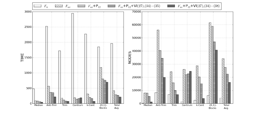
Figure 3: Summary of computational results carried out in the paper.

The capacities were randomly generated in $\displaystyle[\min_{i}W_{i},{(1/2)}\sum_{i\in A}W_{i}]$. This generation procedure does not ensure in all cases feasible instances, as capacity constraints can be very tight for problems with a low number of hubs ($n=3,5$). Overall, in our experiments we got, initially 10 infeasible instances out of 75 (13.3%). These instances were replaced by new feasible ones (generated with the same capacity structure). Hence, the reader may observe that the generation procedure gives tight capacity constraints.

First of all, and for the sake of readability, we present in Figure 3 a summary of our computational results. A full description of those results is also included in Tables 1-6.

Figure 3 shows average results for each one of the considered problem types (different $\lambda$-vectors). The left chart refers to average CPU times and the right chart to the number of explored nodes of the B&B tree. Both charts contain the same number of blocks standing for the different types of $\lambda$-vectors plus and additional block (Total Avg.) for the consolidated average of all $\lambda$-vectors. Each block compares the behavior of the different formulations ($F_{\bar{u}}$,$F_{uv}$) and their strengthening (variable fixing and valid inequalities). The heading explains the meaning of bars within each block: $F_{\bar{u}}$ and $F_{uv}$ stand for the corresponding formulations; $F_{uv}$+P₁₂ when the two preprocesses $P_{1}(h)$ and $P_{2}(h)$ are applied; and $F_{uv}$+P₁₂+VI when the Valid Inequalities are added as well, denoted with their corresponding references.

Analyzing this figure we observe the improvement obtained with $F_{uv}$ and its strengthening as compared with $F_{\bar{u}}$ or even $F_{uv}$ alone. Actually, the overall reduction in running time with respect to the initial formulation is above $89\%$.

Next, focusing in the best model, namely $F_{uv}+P_{12}+$VI(29),(• ‣ 3.2.2)-(40), we observe that the most time consuming problem is the one with $\lambda$-vector given by $\{0,1\}$-blocks with a significant difference with respect to the remaining $\lambda$-vectors. The second most time consuming problem corresponds with the Antitrimmean. Similar conclusions, regarding the number of nodes, are obtained looking at the right chart of Figure 3. It is worth mentioning that although the formulation $F_{\bar{u}}$ provides the worst computational times, it is the one that reports the lowest number of nodes in the B&B tree. This fact is explained because $F_{\bar{u}}$ has a larger number of variables than $F_{uv}$ which results in more difficult LP relaxations in each node of the B&B tree.

In spite of that Figure 3 shows the general overview of our computational results, we also include in the following a more detailed analysis based on Tables 1$-$6.

Tables 1 and 2 report the results of the formulations and different preprocessing phases developed in this paper for the CSA-OMHLP. The first column of these tables describes the different $\lambda$-vectors in the study, the second and third columns report the size of the instances and the number of hubs to be located, respectively. The following three columns correspond to some of the computational results obtained by solving the CSA-OMHLP with $F_{\bar{u}}$ formulation. The next three columns correspond to Formulation $F_{uv}$, and the rest of the columns to the latter formulation plus the two preprocessing procedures, i.e $F_{uv}$+P₁+P₂. Columns RGAP, Nodes and Time stand for the averages of: the gap in the root node, number of nodes in the B&B tree and the CPU time in seconds; the time was limited to two hours of CPU. To obtain a general idea of the comparisons among these averaged values, for the results in the column Time and for different formulations and/or valid inequalities applied, we have accounted the value 7200 seconds for those instances that exceed the time limit. A superindex in their corresponding averaged time value states the number of instances exceeding the CPU time limit; in the same way, the values used to computed the average of the column Nodes have been the number of nodes of the B&B tree when the CPU time limit was reached.

The column Fixed gives the percentage of variables that have been fixed after the Preprocessing Phases 1 and 2. Column Cuts provides the number of the lower and upper bounds over the variables $v$ added to the model, after running the corresponding preprocessing phases. Finally, T. prep. reports the CPU time in seconds of the corresponding preprocessing phases and column T. total reports the overall CPU time in seconds to solve the problem including the corresponding preprocessing phase. The rows Average provide the averaged results among all the tested instances for each problem and TOTAL with respect to the overall set of instances.

Tables 1 and 2 show, as a general trend, that the CPU time increases similarly, for all choices of the $\lambda$-vector, with the size of the instances. We can see that 69 instances required more than two hours to be solved using Formulation $F_{\bar{u}}$, however the remaining two analyzed ways to solve this problem were able to solve all the instances within the CPU time limit, except in a few cases for the Antitrimmean and $\{0,1\}$-blocks problem types. Regarding the running times for the different types of problems, we can see that Anti-TrimMean and Blocks have been the problems that need more time to be solved. In any case, we observed that there is a considerable reduction of the running times from the original formulation to the improved formulation, and after applying the preprocessing phases. From tables 1 and 2, one can remark that, Formulation $F_{uv}$ with Preprocessing Phases 1 and 2 provides better results, with a reduction of around a 86% of the time with respect to Formulation $F_{\bar{u}}$ (taking into account that the latter formulation was not able to solve all the studied instances before the time limit was exceeded). Moreover, the reduction of the running times with respect to Formulation $F_{uv}$ (without preprocessing phases) is around 32 %.

As for the comparison between RGAP’s, we observe that the average gap of the linear relaxation after preprocessing reduces around 32% from the original formulation (Formulation $F_{\bar{u}}$) to Formulation $F_{uv}$ with Preprocessing Phases 1 and 2. In any case, it is also worth noting that the gap from the original formulation to the improved formulation (without any preprocessing phase) is reduced around 9%, what implies that even though this improved formulation uses much less number of variables, it provides a better RGAP.

Tables 3 and 4 present several improvements to Formulation $F_{uv}$ with Preprocessing Phases 1 and 2. In particular, the second, third and fourth blocks of columns summarize the results when the combination of valid inequalities (29)-(31); (29),(• ‣ 3.2.2)-(• ‣ 3.2.2) and (29),(• ‣ 3.2.2)-(• ‣ 3.2.2) are added to this formulation, respectively. In general, we can see that the latter combination provides the best results. In particular, there is an improvement of 7 % of the running times with respect to Formulation $F_{uv}$ with Preprocessing Phases 1 and 2. Moreover, with respect to the number of nodes the improvement is around 15%, but the RGAP is similar for all the analyzed reinforcements.

Since the best behavior observed was obtained with reinforcement given by (29), (• ‣ 3.2.2)-(• ‣ 3.2.2), in the rest of our tests we have used this configuration to make further strengthening. Tables 5 and 6 present several improvements to the Formulation $F_{uv}$ with Preprocessing Phases 1 and 2 and valid inequalities (29), (• ‣ 3.2.2)-(• ‣ 3.2.2). In particular, the second, third and fourth blocks of columns report the results after including the family of valid inequalities (38), (38)-(39) and (38)-(40), respectively. These tables show that the best results are obtained when all valid inequalities, (38)-(40), are added to the current configuration; with an improvement of 18% in the running time, 28% in the number of nodes and 12 % in the RGAP.

The overall conclusion of our experiment is that in order to solve CSA-OMHLP the best combination of formulation and strengthening is to use $F_{uv}+P_{12}+$(29)$+$(• ‣ 3.2.2)$+$(• ‣ 3.2.2)$+$(38)$+$(40). This configuration allows to solve medium size instances within 10 minutes of CPU time.

5 Concluding remarks

This paper can be considered as an initial attempt to address the capacitated single-allocation ordered hub location problem. The formulations, strengthening and preprocessing phases developed in this paper provide a promising approach to solve the above mentioned problem although so far only medium size problems are reasonably well-solved. Thus, this work opens interesting possibilities to study-and-develop ad-hoc solution procedures that allow us to consider larger size instances of this problem. Moreover, it also points out the possibility of developing heuristics approaches that will give good solutions in competitive running times. All in all, this paper shows the usefulness of using covering formulations and their corresponding strengthening for solving capacitated versions of ordered hub location problems.

Table 1: Computational results for Formulations $F_{\bar{u}}$ vs $F_{uv}$ with preprocessing.

	n	p	Formulation $F_{\bar{u}}$			Formulation $F_{uv}$			Formulation $F_{uv}$ + P1+P2
			RGAP	Nodes	Time	RGAP	Nodes	Time	RGAP	Nodes	T total	T. prep	Fixed	Cuts
MEDIAN	15	3	17,56	17	7,9	17,56	240	1,8	15,16	195	1,4	1,4	2,4	240
	15	5	7,60	3	3,8	7,60	230	0,8	6,78	177	0,7	1,2	1,4	180
	15	8	8,49	1	1,0	8,49	259	0,6	4,39	185	0,4	1,0	0,8	133
	20	3	19,54	75	69,5	19,54	505	6,3	16,31	472	5,8	3,1	3,9	405
	20	8	6,05	1	3,9	6,05	1024	4,2	5,49	1122	3,8	2,2	1,9	215
	20	10	2,88	1	3,1	2,88	591	1,9	2,59	560	1,6	1,7	1,8	181
	25	3	19,00	1.051	509,5	19,00	478	21,2	15,21	408	18,5	8,9	7,2	800
	25	8	6,77	1	12,7	6,77	4239	30,9	5,95	6177	33,6	5,2	4,1	459
	25	10	13,10	15	48,6	13,10	6656	33,4	6,31	4686	26,0	5,2	3,4	435
	28	3	21,86	270	322,7	21,86	2052	66,8	16,01	2246	76,6	13,2	10,5	960
	28	8	9,21	143	415,6	9,21	16820	165,5	8,15	10560	97,4	7,7	6,5	597
	28	10	7,36	129	321,3	7,36	27440	193,1	6,78	32680	243,1	6,7	3,8	396
	30	3	32,36	1.416	4007,0(1)	32,32	3701	167,7	20,92	2564	127,8	18,8	11,0	1128
	30	8	18,69	360	1346,0	18,69	39430	455,5	10,86	36790	437,3	12,8	6,2	817
	30	10	9,18	22	186,3	9,18	18420	176,8	6,98	20130	207,6	11,4	5,4	685
	Average		13,30	234	483,9	13,30	8139	88,4	9,90	7930	85,4	6,7	4,7	509
ANTITRIMMEAN	15	3	23,75	150	33,6	23,75	614	2,8	17,62	645	2,0	1,4	6,1	164
	15	5	13,93	99	12,9	13,93	1039	2,2	8,38	803	1,4	1,1	4,3	104
	15	8	13,20	29	9,4	13,20	618	1,1	6,82	724	0,9	1,0	2,6	91
	20	3	23,50	2448	272,0	23,50	2032	16,8	17,44	1150	9,2	3,1	9,8	273
	20	8	9,45	379	79,9	9,45	4637	11,9	7,66	3009	7,8	2,2	5,2	126
	20	10	4,66	73	36,4	4,66	3150	6,9	4,28	3394	6,4	1,7	4,4	123
	25	3	24,64	12130	2037,0	24,64	1984	53,8	17,29	1218	29,0	8,9	18,9	540
	25	8	10,32	590	344,4	10,32	6411	40,2	7,91	6841	33,3	5,2	10,4	324
	25	10	17,25	13650	1217,0	17,25	27180	115,1	9,81	25390	102,1	5,2	8,6	330
	28	3	25,94	16460	5111,0(1)	25,94	26600	957,1	17,36	7432	168,4	13,2	22,1	717
	28	8	13,58	12390	5688,0(3)	13,52	42860	381,4	10,67	34800	271,1	7,8	16,8	301
	28	10	10,95	13830	3524,0(2)	10,92	262500	1595,0	9,14	131900	832,1	6,7	9,7	242
	30	3	36,85	11110	6584,0(4)	35,55	15670	591,0	21,74	7220	271,6	18,8	27,2	770
	30	8	23,80	19960	7200,0(5)	23,72	299700	3402,0	14,48	273600	2896,0	12,8	15,8	598
	30	10	13,53	21200	5707,0(3)	13,50	145000	1310,0	10,56	109700	863,2	11,4	15,4	464
	Average		17,70	8300	2523,8	17,60	56000	565,8	12,10	40522	366,3	6,7	11,8	345
TRIMMEAN	15	3	19,46	177	22,9	17,43	1066	2,1	16,44	729	1,4	1,4	0,8	76
	15	5	11,26	38	13,6	8,65	1209	1,1	8,58	646	0,7	1,2	0,8	67
	15	8	8,72	4	3,6	7,88	510	0,4	7,88	322	0,3	1,0	0,3	20
	20	3	20,77	5452	335,9	19,38	1047	7,0	17,65	1022	6,2	3,1	1,9	132
	20	8	12,10	1107	96,7	9,48	6847	13,4	9,08	4512	7,9	2,2	1,2	88
	20	10	8,88	63	36,7	6,17	2309	4,4	5,97	1620	2,7	1,7	0,9	58
	25	3	19,74	18180	2157,0	18,78	2039	31,4	16,87	2081	25,1	8,9	3,2	260
	25	8	10,55	5365	804,0	8,94	61330	211,7	8,63	21460	74,2	5,2	2,2	140
	25	10	13,58	1186	225,4	12,34	2642	9,6	12,28	1760	6,5	5,2	1,9	117
	28	3	21,50	18050	4959,0(1)	20,54	8611	149,2	17,49	3800	69,6	13,3	3,9	243
	28	8	12,23	12740	2304,0	10,74	47430	309,6	10,24	20290	130,9	7,7	3,8	234
	28	10	11,27	6731	1467,0	9,25	35750	178,7	9,171	14770	69,3	6,7	2,8	174
	30	3	26,67	9820	6506,0(4)	25,15	9904	294,1	22,08	3302	124,4	18,8	5,6	358
	30	8	17,04	10390	3766,0(1)	15,44	90810	868,1	15,09	54920	483,1	12,8	3,6	243
	30	10	11,37	14330	3181,0	9,44	92100	690,0	9,40	107100	757,0	11,4	3,2	227
	Average		15,00	6909	1725,3	13,30	24240	184,7	12,50	15889	117,3	6,7	2,4	163

Table 2: Computational results for Formulations $F_{\bar{u}}$ vs $F_{uv}$ with preprocessing(II).

	n	p	Formulation $F_{\bar{u}}$			Formulation $F_{uv}$			Formulation $F_{uv}$ + P1+P2
			RGAP	Nodes	Time	RGAP	Nodes	Time	RGAP	Nodes	T total	T. prep	Fixed	Cuts
CENTER	15	3	23,84	159	36,7	22,87	780	2,5	16,90	489	0,9	1,4	5,1	0
	15	5	16,54	194	24,5	14,97	1374	1,9	8,48	808	0,9	1,1	4,7	0
	15	8	19,85	84	21,1	16,45	622	1,0	8,83	501,0	0,6	1,0	3,9	0
	20	3	21,36	1.225	347,5	20,76	1118	9,9	16,72	1017	4,8	3,2	8,9	0
	20	8	14,30	775	224,6	12,48	4195	8,9	11,58	3712	6,2	2,2	4,9	0
	20	10	12,16	438	88,6	9,32	2675	5,9	8,817	3019	5,3	1,7	3,8	0
	25	3	21,97	1785	1626,0	21,58	1948	31,2	14,57	938	12,3	8,9	18,4	0
	25	8	15,70	2763	1663,0	14,50	45250	161,6	11,33	26520	87,4	5,2	10,7	0
	25	10	27,76	1901	1525,0	25,91	5302	21,2	16,16	5134	17,7	5,2	11,1	0
	28	3	22,50	2698	5939,0(2)	21,30	5756	121,0	17,56	4172	66,8	13,2	18,5	0
	28	8	18,35	1931	6031,0(2)	16,63	30380	198,0	15,77	29450	170,1	7,8	11,5	0
	28	10	16,65	3266	6621,0(3)	15,09	54930	272,6	14,53	48120	218,4	6,7	8,6	0
	30	3	42,50	1725	6234,0(4)	31,02	8074	293,5	19,75	6536	147,3	18,7	24,4	0
	30	8	32,41	1035	7200,0(5)	27,59	134300	1096,0	14,63	103700	786,6	12,8	21,2	0
	30	10	17,93	2533	6563,0(4)	16,20	93330	646,2	11,77	96140	593,6	11,4	17,3	0
	Average		21,60	1501	2945,8	19,10	26002	191,4	13,80	22017	141,3	6,7	11,5	0
K-CENTRUM	15	3	26,74	148	39,9	23,07	1031	3,0	17,60	588	1,8	1,4	1,5	143
	15	5	16,81	7	14,5	10,97	1093	1,9	7,91	498	1,0	1,1	1,3	161
	15	8	15,68	1	3,1	8,49	259	0,6	4,39	185	0,4	1,0	0,8	133
	20	3	27,98	1995	526,5	25,45	2426	17,0	18,23	1528	9,1	3,1	2,6	247
	20	8	14,46	841	146,9	9,49	5136	12,7	7,12	2902	6,2	2,2	1,7	144
	20	10	9,53	356	67,7	4,84	4255	7,7	4,04	3705	5,9	1,7	1,2	127
	25	3	29,31	4964	2562,0	27,24	2727	49,1	17,48	2693	32,3	8,9	5,3	442
	25	8	14,14	52	476,7	9,79	5928	38,5	7,33	3910	23,2	5,2	2,7	342
	25	10	20,63	1976	512,9	14,78	13330	64,9	7,34	12820	52,6	5,2	2,2	358
	28	3	29,78	2991	6343,0(3)	27,99	13280	264,2	17,17	4971	111,3	13,3	6,2	466
	28	8	15,97	9132	4372,0(1)	12,12	60840	531,5	9,44	21180	178,9	7,8	3,7	431
	28	10	14,09	6460	2576,0(1)	9,11	73800	526,4	7,63	35460	228,2	6,7	2,7	324
	30	3	41,03	671	7200,0(5)	36,42	18830	616,8	21,74	4588	187,6	18,7	7,3	720
	30	8	25,04	5859	6632,0(4)	21,06	174500	2047,0	12,20	171500	1830,0	12,8	4,4	695
	30	10	14,74	2560	2536,0	10,24	53280	506,9	7,63	37330	340,0	11,4	4,8	648
	Average		21,10	2534	2267,7	16,70	28714	312,5	11,20	20257	200,6	6,7	3,2	359
BLOCKS	15	3	19,46	94	15,5	19,46	2210	8,9	15,97	1729	3,8	1,45	8,7	91
	15	5	12,24	33	10,9	11,79	1122	3,7	8,08	860	2,4	1,2	6,7	117
	15	8	12,71	9	7,6	12,37	1065	1,8	6,25	715	1,1	1,0	3,3	76
	20	3	21,09	606	113,0	20,86	3721	30,7	17,58	5777	24,7	3,2	16,1	219
	20	8	8,55	402	67,3	8,55	12670	41,3	7,46	8064	20,4	2,2	4,8	116
	20	10	4,70	97	33,2	4,32	3590	8,4	4,00	4585	9,0	1,7	3,7	122
	25	3	21,51	4850	983,7	21,27	5637	114,4	16,45	4087	59,1	8,9	27,5	484
	25	8	9,99	1675	429,2	9,94	13400	115,0	8,12	12050	89,3	5,2	17,4	260
	25	10	17,57	6874	1021,0	17,40	46270	216,9	10,01	40870	177,5	5,2	7,4	268
	28	3	22,45	5627	2887,0	22,45	9111	472,4	17,16	8569	267,1	13,4	48,3	482
	28	8	10,44	14490	2687,0	10,25	96840	1515,0	9,32	54910	745,0	7,7	24,1	357
	28	10	9,39	13040	3181,0(1)	9,26	233200	2683,0	8,67	184700	1601,0	6,7	15,4	218
	30	3	33,18	10180	5755,0(2)	33,04	10250	753,4	22,39	12840	703,5	18,9	56,4	664
	30	8	21,41	15590	6438,0(4)	21,46	201400	6587,0	12,95	193300	5016,0(3)	12,9	24,5	511
	30	10	11,90	18420	4144,0(2)	11,66	283700	5113,0	9,45	256600	3402,0(1)	11,51	23,28	465
	Average		15,80	6132	1851,6	15,60	61612	1177,7	11,60	52644	808,1	6,8	19,2	297
	TOTAL		17,40	4268	1966,3	15,90	34118	420,1	11,80	26543	286,5	6,7	8,8	279

Table 3: Computational results for Formulation$F_{uv}$ with Valid Inequalities (I)

	n	p	P1+P${}_{2}=$ P12			P12+V.I.(29)-(31)			P12+V.I.(29),(• ‣ 3.2.2)-(• ‣ 3.2.2)			P12+V.I.(29),(• ‣ 3.2.2)-(• ‣ 3.2.2)
			RGAP	Nodes	time	RGAP	Nodes	time	RGAP	Nodes	time	RGAP	Nodes	time
MEDIAN	15	3	15,16	195	1,4	14,21	199	1,4	14,21	262	1,5	14,21	239	1,4
	15	5	6,78	177	0,7	6,50	154	0,7	6,50	232	0,8	6,50	230	0,8
	15	8	4,39	185	0,4	4,33	110	0,4	4,33	157	0,4	4,34	162	0,5
	20	3	16,31	472	5,8	15,66	379	7,1	15,66	540	7,4	15,66	560	7,3
	20	8	5,49	1122	3,8	4,98	981	4,1	4,98	1189	4,4	4,98	936	3,9
	20	10	2,59	560	1,6	2,33	658	1,9	2,33	654	1,8	2,33	857	2,4
	25	3	15,21	408	18,5	14,79	502	21,3	14,79	490	20,9	14,79	390	19,9
	25	8	5,95	6177	33,6	5,39	1772	16,8	5,39	2994	21,6	5,39	3301	26,5
	25	10	6,31	4686	26,0	5,97	2748	16,1	5,97	3141	18,5	5,97	2734	16,8
	28	3	16,01	2246	76,6	15,72	1968	72,6	15,72	1871	71,5	15,72	2055	71,9
	28	8	8,15	10560	97,4	7,53	5937	62,5	7,53	5999	66,2	7,53	6398	70,4
	28	10	6,78	32680	243,1	6,48	21080	155,2	6,48	16800	136,4	6,48	17930	125,4
	30	3	20,92	2564	127,8	20,60	2300	132,9	20,60	2797	149,9	20,60	2770	142,3
	30	8	10,86	36790	437,3	10,35	31990	448,0	10,35	25920	338,3	10,35	25060	332,7
	30	10	6,98	20130	207,6	6,75	17230	167,8	6,75	15720	160,4	6,75	18130	179,8
	Average		9,90	7930	85,4	9,40	5867	73,9	9,40	5251	66,7	9,40	5450	66,8
ANTI-TRIMMEAN	15	3	17,62	645	2,0	17,18	559	1,9	17,18	709	2,1	17,18	556	2,0
	15	5	8,38	803	1,4	8,36	823	1,6	8,36	615	1,4	8,36	705	1,5
	15	8	6,82	724	0,9	6,82	808	0,9	6,82	723	0,9	6,82	736	1,0
	20	3	17,44	1150	9,2	17,00	1471	11,4	17,00	1455	11,7	17,00	1370	10,9
	20	8	7,66	3009	7,8	7,54	2684	7,1	7,54	2716	7,6	7,54	2709	7,7
	20	10	4,28	3394	6,4	4,28	2663	6,1	4,28	2192	5,1	4,28	2574	5,7
	25	3	17,29	1218	29,0	16,95	1294	31,7	16,95	1314	33,9	16,95	1167	28,5
	25	8	7,91	6841	33,31	7,74	5315	30,7	7,74	3127	22,7	7,74	5038	30,4
	25	10	9,81	25390	102,1	9,76	11640	55,2	9,76	12560	61,8	9,76	13830	66,2
	28	3	17,36	7432	168,4	17,10	6343	155,4	17,10	7032	164,6	17,10	7531	168,8
	28	8	10,67	34800	271,1	10,63	23080	204,8	10,63	21210	191,3	10,63	20850	188,2
	28	10	9,141	131900	832,1	9,11	92660	659,0	9,11	81600	634,5	9,11	93700	705,6
	30	3	21,74	7220	271,6	21,47	3502	164,5	21,47	4853	204,9	21,47	4873	190,1
	30	8	14,48	273600	2896,0	14,36	183100	2022,0	14,36	204500	2250,0	14,36	258800	3026,0
	30	10	10,56	109700	863,2	10,50	99160	837,6	10,50	94870	784,8	10,50	103700	898,1
	Average		12,10	40522	366,3	11,90	29007	279,3	11,90	29298	291,8	11,90	34543	355,4
TRIMMEAN	15	3	16,44	729	1,4	16,19	677	1,4	16,19	733	1,4	16,19	789	1,5
	15	5	8,58	646	0,7	8,39	566	0,7	8,39	550	0,8	8,39	489	0,7
	15	8	7,88	322	0,3	7,85	353	0,3	7,85	349	0,3	7,85	366	0,3
	20	3	17,65	1022	6,2	17,60	871	6,5	17,60	977	6,2	17,60	929	6,8
	20	8	9,08	4512	7,9	9,00	4519	8,3	9,00	4508	7,9	9,00	4476	8,4
	20	10	5,97	1620	2,7	5,95	1402	2,5	5,95	1353	2,5	5,95	1444	2,6
	25	3	16,87	2081	25,1	16,83	1844	24,1	16,83	1879	26,8	16,83	1486	22,5
	25	8	8,63	21460	74,2	8,40	13420	54,4	8,40	14300	56,4	8,40	15390	59,5
	25	10	12,28	1760	6,5	12,14	1106	4,8	12,14	1384	5,7	12,14	1251	5,6
	28	3	17,49	3800	69,6	17,48	4117	80,5	17,48	4005	71,0	17,48	4458	80,8
	28	8	10,24	20290	130,9	9,97	15890	111,4	9,97	17340	119,1	9,97	16910	119,1
	28	10	9,17	14770	69,3	8,92	8775	41,6	8,92	9241	44,4	8,92	10490	49,7
	30	3	22,08	3302	124,4	22,05	4052	157,8	22,05	4356	157,0	22,05	3925	147,3
	30	8	15,09	54920	483,1	14,99	45860	450,8	14,99	50140	486,9	14,99	52040	514,7
	30	10	9,36	107100	757,0	9,17	42140	316,1	9,17	36570	275,1	9,17	36480	263,3
	Average		12,50	15889	117,3	12,30	9706	84,1	12,30	9846	84,1	12,30	10062	85,5

Table 4: Computational results for Formulation$F_{uv}$ with Valid Inequalities (I)

	n	p	P1+P${}_{2}=$ P12			P12+V.I.(29)-(31)			P12+V.I.(29),(• ‣ 3.2.2)-(• ‣ 3.2.2)			P12+V.I.(29),(• ‣ 3.2.2)-(• ‣ 3.2.2)
			RGAP	Nodes	time	RGAP	Nodes	time	RGAP	Nodes	time	RGAP	Nodes	time
CENTRUM	15	3	16,90	489	0,9	16,90	429	0,9	16,90	468	0,9	16,90	701	1,1
	15	5	8,48	809	0,9	8,47	788	0,9	8,47	800	1,0	8,47	759	1,0
	15	8	8,83	501	0,6	8,83	495	0,6	8,83	554	0,6	8,83	556	0,6
	20	3	16,72	1017	4,8	16,70	840	4,6	16,70	1028	4,7	16,70	876	4,5
	20	8	11,58	3712	6,2	11,58	3185	5,9	11,58	3778	6,6	11,58	4408	7,9
	20	10	8,82	3019	5,3	8,82	2430	4,9	8,82	2377	4,9	8,82	2044	4,7
	25	3	14,57	938	12,3	14,56	956	14,3	14,56	821	12,5	14,56	983	13,6
	25	8	11,33	26520	87,4	11,33	25490	89,2	11,33	26310	95,2	11,33	30540	107,2
	25	10	16,16	5134	17,7	16,16	3933	15,3	16,16	4357	15,9	16,16	5271	19,2
	28	3	17,56	4172	66,8	17,55	5275	75,3	17,55	4087	69,8	17,55	5190	86,6
	28	8	15,77	29450	170,1	15,77	25760	157,3	15,77	30410	185,7	15,77	25740	160,5
	28	10	14,53	48120	218,4	14,53	49170	233,4	14,53	62630	298,0	14,53	53050	269,0
	30	3	19,75	6536	147,3	19,73	4810	124,0	19,73	6142	151,6	19,73	5994	151,6
	30	8	14,63	103700	786,6	14,63	86370	680,3	14,63	113900	904,5	14,63	108300	965,3
	30	10	11,77	96140	593,6	11,77	128200	882,8	11,77	108700	766,9	11,77	94490	675,7
	Average		13,8	22017	141,3	13,8	22542	152,7	13,80	24424	167,9	13,80	22594	164,6
K-CENTRUM	15	3	17,60	588	1,8	17,58	659	1,9	17,58	707	2,0	17,58	783	1,9
	15	5	7,91	498	1,0	7,85	653	1,3	7,85	547	1,2	7,85	635	1,2
	15	8	4,40	185	0,4	4,33	110	0,4	4,33	157	0,4	4,34	162	0,4
	20	3	18,23	1.528	9,1	18,22	1590	10,6	18,22	1287	10,0	18,22	1777	10,7
	20	8	7,12	2.902	6,2	7,09	3290	7,8	7,09	2568	6,2	7,09	2821	6,7
	20	10	4,04	3705	5,9	4,03	2973	5,2	4,03	2769	4,8	4,03	3045	5,4
	25	3	17,48	2693	32,3	17,47	1764	28,4	17,47	1537	26,6	17,47	1639	28,0
	25	8	7,33	3910	23,2	7,30	3239	21,0	7,30	3488	24,3	7,30	3264	23,5
	25	10	7,34	12820	52,6	7,28	12730	51,9	7,28	11770	49,6	7,28	11330	48,8
	28	3	17,17	4971	111,3	17,16	4126	103,2	17,16	4417	106,4	17,16	4146	108,7
	28	8	9,44	21180	178,9	9,39	17390	158,4	9,39	14370	140,5	9,39	14120	139,8
	28	10	7,63	35460	228,2	7,54	39050	276,9	7,54	38760	268,8	7,54	34770	247,2
	30	3	21,74	4588	187,6	21,72	4740	188,6	21,72	4069	169,9	21,72	4437	194,9
	30	8	12,20	171500	1830,0	12,14	149900	1737,0	12,15	218900	2710,0	12,14	114200	1343,0
	30	10	7,63	37330	340,0	7,54	41100	392,6	7,54	34690	332,8	7,54	30780	305,4
	Average		11,20	20257	200,6	11,10	18888	199,0	11,10	22669	256,9	11,10	15194	164,4
BLOCKS	15	3	15,97	1729	3,8	15,86	2184	4,2	15,86	1481	3,7	15,86	2248	4,4
	15	5	8,08	860	2,4	7,98	1085	2,8	7,98	877	2,4	7,98	877	2,7
	15	8	6,25	715	1,1	6,23	748	1,2	6,23	772	1,1	6,23	726	1,1
	20	3	17,58	5777	24,7	17,41	3515	19,7	17,41	4382	19,3	17,41	4007	21,0
	20	8	7,46	8064	20,4	7,40	5603	15,8	7,40	6327	16,1	7,40	5217	15,8
	20	10	4,00	4585	9,0	3,98	4308	8,6	3,98	4091	8,5	3,98	3505	7,8
	25	3	16,45	4087	59,1	16,28	4489	67,7	16,28	4821	65,1	16,28	4434	63,9
	25	8	8,12	12050	89,3	8,07	8427	64,9	8,07	7338	54,5	8,07	7836	64,9
	25	10	10,01	40870	177,5	9,99	49940	199,6	9,99	36030	155,2	9,99	35520	158,8
	28	3	17,16	8569	267,1	17,11	11070	312,0	17,11	5840	220,4	17,11	5934	210,7
	28	8	9,32	54910	745,0	9,14	47500	723,0	9,14	54830	749,3	9,14	43450	580,5
	28	10	8,67	184700	1601,0	8,61	124900	1118,0	8,61	149500	1385,0	8,61	140900	1323,0
	30	3	22,39	12840	703,5	22,20	10580	572,6	22,20	10520	542,8	22,20	9661	517,0
	30	8	12,95	193300	5016,0(3)	12,76	261900	6298,0(4)	12,75	197700	4858,0(3)	12,74	187400	4854,0(3)
	30	10	9,45	256600	3402,0(1)	9,29	248300	3476,0(1)	9,29	215800	3277,0(3)	9,30	253000	3586,0(1)
	Average		11,60	52644	808,1	11,50	52303	858,9	11,50	46687	757,2	11,50	46981	760,8
TOTAL			11,80	26543	286,5	11,70	23052	274,7	11,70	23029	270,8	11,70	22470	266,2

Table 5: Computational results for Formulation$F_{uv}$ with Valid Inequalities (II)

	n	p	P12+V.I.(29),(• ‣ 3.2.2)-(• ‣ 3.2.2)			P12+V.I.(29),(• ‣ 3.2.2)-(38)			P12+V.I.(29),(• ‣ 3.2.2)-(39)			P12+V.I.(29),(• ‣ 3.2.2)-(40)
			RGAP	Nodes	time	RGAP	Nodes	time	RGAP	Nodes	time	RGAP	Nodes	time
MEDIAN	15	3	14,21	239	1,4	7,71	168	2,3	7,71	197	2,5	7,63	210	2,3
	15	5	6,50	230	0,8	4,58	122	1,4	4,58	117	1,4	4,60	132	1,6
	15	8	4,33	162	0,5	4,04	166	0,7	4,04	150	0,8	4,04	153	0,9
	20	3	15,66	560	7,3	7,08	220	11,9	7,08	345	12,3	7,16	281	12,7
	20	8	4,98	936	3,9	4,38	262	4,4	4,38	600	5,4	4,36	318	4,3
	20	10	2,33	857	2,4	2,24	354	3,2	2,21	328	2,9	2,21	273	2,9
	25	3	14,79	390	19,9	7,52	429	44,5	7,512	319	42,9	7,52	393	42,7
	25	8	5,39	3301	26,5	4,03	521	17,8	4,02	486	18,5	4,02	405	16,3
	25	10	5,97	2734	16,8	5,48	1177	15,9	5,48	1265	16,4	5,48	1175	17,3
	28	3	15,72	2055	71,9	6,75	320	88,1	6,75	414	82,8	6,76	322	85,7
	28	8	7,53	6398	70,4	5,15	1627	47,6	5,13	1294	42,9	5,15	1781	49,3
	28	10	6,48	17930	125,4	4,73	4394	57,9	4,73	4914	62,8	4,70	3674	50,2
	30	3	20,60	2770	142,3	13,90	868	143,6	13,67	846	160,5	13,71	889	157,5
	30	8	10,35	25060	332,7	8,19	4083	111,7	8,19	3348	96,0	8,24	4593	127,6
	30	10	6,75	18130	179,8	5,49	4232	77,7	5,49	3426	65,9	5,49	3.64	76,5
	Average		9,40	5450	66,8	6,10	1263	41,9	6,10	1203	40,9	6,10	1231	43,2
ANTI-TRIMMEAN	15	3	17,18	556	2,0	15,28	467	2,9	15,28	526	3,3	15,28	510	2,9
	15	5	8,36	705	1,5	8,02	562	1,9	8,02	432	1,7	8,02	441	1,8
	15	8	6,82	736	1,0	6,71	669	1,3	6,71	686	1,2	6,71	733	1,3
	20	3	17,00	1370	10,9	14,55	737	15,6	14,55	1027	15,9	14,55	1008	16,6
	20	8	7,54	2709	7,7	7,31	1876	7,7	7,31	1684	7,1	7,31	2041	7,9
	20	10	4,28	2574	5,7	4,21	2168	6,2	4,21	2367	6,4	4,21	2720	7,1
	25	3	16,95	1167	28,5	15,41	1016	47,5	15,41	1055	50,6	15,41	800	50,9
	25	8	7,74	5038	30,4	7,03	1903	22,9	7,03	2066	23,7	7,03	2664	26,7
	25	10	9,76	13830	66,2	9,69	13360	71,2	9,69	10670	57,1	9,69	13710	70,3
	28	3	17,10	7531	168,8	14,25	2024	112,8	14,25	1943	114,0	14,25	2380	119,8
	28	8	10,63	20850	188,2	10,34	11240	133,7	10,34	12110	144,9	10,34	10960	128,0
	28	10	9,11	93700	705,6	8,89	66920	519,5	8,89	61180	522,6	8,89	69100	527,7
	30	3	21,47	4873	190,1	18,10	4082	295,5	18,10	2724	255,0	18,10	2702	239,1
	30	8	14,36	258800	3026,0	13,96	135200	1701,0	13,96	124200	1576,0	13,96	123600	1526,0
	30	10	10,50	103700	898,1	10,26	55810	497,4	10,26	61050	566,9	10,33	65660	606,6
	Average		11,90	34543	355,4	10,90	19869	229,1	10,90	18915	223,1	10,90	19935	222,2
TRIMMEAN	15	3	16,19	789	1,5	14,68	647	2,1	14,56	546	2,3	14,56	437	2,2
	15	5	8,39	489	0,7	7,71	525	1,1	7,71	487	1,0	7,71	513	1,1
	15	8	7,85	366	0,3	7,79	342	0,5	7,79	417	0,6	7,79	384	0,5
	20	3	17,60	929	6,8	15,17	978	11,8	15,02	648	11,7	15,02	861	12,8
	20	8	9,01	4476	8,4	8,68	4139	8,5	8,59	3603	8,5	8,59	3434	8,5
	20	10	5,95	1444	2,6	5,83	1302	3,6	5,80	1251	3,8	5,80	1464	4,2
	25	3	16,83	1486	22,5	15,84	1671	39,2	15,74	1077	38,9	15,74	1148	39,4
	25	8	8,40	15390	59,5	8,24	12770	57,5	8,19	11340	53,7	8,19	11400	54,1
	25	10	12,14	1251	5,6	12,07	1382	9,5	12,07	1249	8,9	12,07	1155	9,0
	28	3	17,48	4458	80,8	15,77	2371	88,3	15,60	1727	83,5	15,60	1721	82,9
	28	8	9,97	16910	119,1	9,63	11070	93,3	9,39	9072	81,6	9,39	7802	74,6
	28	10	8,92	10490	49,7	8,76	9234	55,4	8,76	10090	57,1	8,76	10920	63,8
	30	3	22,05	3925	147,3	19,80	3477	200,0	19,69	2634	189,6	19,69	2233	177,0
	30	8	14,99	52040	514,7	14,54	33800	348,4	14,52	29400	326,1	14,52	29980	339,6
	30	10	9,17	36480	263,3	8,63	26750	205,3	8,63	26950	229,9	8,63	27860	228,9
	Average		12,30	10062	85,5	11,50	7364	75,0	11,50	6699	73,1	11,50	6754	73,3

Table 6: Computational results for Formulation$F_{uv}$ with Valid Inequalities (II)bis

	n	p	P12+V.I.(29),(• ‣ 3.2.2)-(• ‣ 3.2.2)			P12+V.I.(29),(• ‣ 3.2.2)-(38)			P12+V.I.(29),(• ‣ 3.2.2)-(39)			P12+V.I.(29),(• ‣ 3.2.2)-(40)
			RGAP	Nodes	time	RGAP	Nodes	time	RGAP	Nodes	time	RGAP	Nodes	time
CENTRUM	15	3	16,90	701	1,1	16,32	574	1,6	16,32	576	1,6	16,32	513	1,6
	15	5	8,47	759	1,0	8,45	769	1,3	8,45	850	1,4	8,45	850	1,5
	15	8	8,83	556	0,6	8,81	577	0,8	8,78	582	0,9	8,78	437	0,9
	20	3	16,70	876	4,5	15,94	579	7,1	15,94	649	7,0	15,94	705	6,9
	20	8	11,58	4408	7,9	11,57	4061	7,9	11,56	3902	8,3	11,56	3725	7,8
	20	10	8,82	2044	4,7	8,82	2044	5,4	8,82	2739	6,2	8,82	2389	5,6
	25	3	14,56	983	13,6	14,27	689	19,0	14,27	669	19,8	14,27	750	19,9
	25	8	11,33	30540	107,2	11,29	29000	103,6	11,29	25290	96,5	11,29	28560	104,6
	25	10	16,16	5271	19,2	16,15	4339	18,4	16,15	4335	18,6	16,15	5226	21,4
	28	3	17,55	5190	86,6	16,87	2660	74,6	16,87	2788	79,9	16,87	2997	83,0
	28	8	15,77	25740	160,5	15,75	26910	175,6	15,75	25320	179,3	15,75	26240	173,8
	28	10	14,53	53050	269,0	14,52	57390	296,1	14,52	58690	314,7	14,52	50760	265,1
	30	3	19,73	5994	151,6	18,36	4419	183,1	18,36	3236	148,0	18,36	4846	190,2
	30	8	14,63	108300	965,3	14,59	119500	1068,0	14,59	110300	1094,0	14,59	133400	1228,0
	30	10	11,77	94490	675,7	11,77	94490	678,4	11,77	91310	700,3	11,77	107000	806,9
	Average		13,80	22594	164,6	13,60	23200	176,1	13,60	22082	178,4	13,60	24560	194,5
K-CENTRUM	15	3	17,58	783	1,9	14,72	678	3,3	14,49	502	3,2	14,49	594	3,4
	15	5	7,85	6345	1,2	6,80	437	1,8	6,58	387	1,8	6,58	358	1,9
	15	8	4,34	162	0,4	4,04	166	0,7	4,04	150	0,8	4,04	153	0,8
	20	3	18,22	1777	10,7	15,52	959	13,3	15,25	847	14,1	15,25	904	13,8
	20	8	7,09	2821	6,7	6,77	1272	6,1	6,62	1260	6,7	6,62	1001	6,4
	20	10	4,03	3045	5,4	3,84	2437	6,0	3,74	1879	5,6	3,74	1950	5,5
	25	3	17,47	1639	28,0	16,17	1404	46,7	16,11	1035	45,3	16,11	1377	50,7
	25	8	7,29	3264	23,5	6,46	1895	23,2	6,30	1777	23,8	6,30	1571	23,1
	25	10	7,28	11330	48,8	7,09	6548	38,5	6,99	5529	36,0	6,99	5793	37,2
	28	3	17,16	4146	108,7	14,52	1557	83,6	14,21	1076	89,4	14,21	904	82,9
	28	8	9,39	14120	139,8	8,345	5935	89,7	8,14	5073	82,3	8,14	5264	84,9
	28	10	7,54	34770	247,2	6,66	26570	206,3	6,51	11410	113,9	6,51	9299	99,6
	30	3	21,72	4437	194,9	17,34	3598	269,3	17,02	2889	237,2	17,02	3989	279,3
	30	8	12,14	114200	1343,0	10,75	17250	291,0	10,66	97400	1434,0	10,77	16090	303,5
	30	10	7,54	30780	305,4	6,60	13560	170,7	6,55	8198	120,1	6,59	8883	133,7
	Average		11,10	15194	164,4	9,70	5618	83,3	9,50	9294	147,6	9,60	3875	75,1
BLOCKS	15	3	15,86	2248	4,4	13,58	2925	6,9	13,55	2611	6,7	13,55	2388	6,7
	15	5	7,98	877	2,7	7,35	785	3,5	7,35	898	3,7	7,35	762	3,4
	15	8	6,23	726	1,1	6,14	678	1,4	6,11	804	1,6	6,11	698	1,5
	20	3	17,41	4007	21,0	14,06	4384	31,1	14,06	4642	31,9	14,06	4712	32,7
	20	8	7,40	5217	15,8	7,12	4646	15,9	7,11	5109	17,8	7,11	4380	15,7
	20	10	3,98	3505	7,8	3,91	2882	8,5	3,89	3016	8,8	3,89	3319	9,5
	25	3	16,28	4434	63,9	14,65	5324	98,9	14,65	4923	91,3	14,65	6696	102,0
	25	8	8,07	7836	64,9	7,39	4695	51,8	7,39	5066	54,5	7,39	5400	57,9
	25	10	9,99	35520	158,8	9,96	34470	151,7	9,96	49260	222,5	9,96	37030	169,3
	28	3	17,11	5934	210,7	14,05	4436	229,0	14,05	5004	290,9	14,05	3642	206,0
	28	8	9,14	43450	580,5	8,61	54300	1787,0	8,61	35590	559,7	8,61	32250	503,8
	28	10	8,61	140900	1323,0	8,20	94410	1013,0	8,20	105800	1150,0	8,20	125300	1328,0
	30	3	22,20	9661	517,0	18,45	7648	623,9	18,45	7766	637,6	18,45	6555	539,6
	30	8	12,74	187400	4854,0(3)	12,26	177000	4807,0(3)	12,17	176000	4400,0(2)	12,19	184600	4494,0(2)
	30	10	9,30	253000	3586,0(1)	9,06	191400	2931,0(1)	9,04	208800	3333,0(1)	9,04	194700	2991,0(1)
	Average		11,50	46981	760,8	10,30	39332	784,0	10,30	41019	720,7	10,30	40829	697,4
TOTAL			11,70	22470	266,2	10,40	16108	231,6	10,30	16536	230,7	10,30	16197	217,6

References

- [1] S. Alumur and B.Y. Kara. Network hub location problems: the state of the art. European Journal of Operational Research, 190(1):1–21, 2008.
- [2] T. Aykin Lagrangian relaxation based approaches to capacitated hub-and-spoke network design problem. European Journal of Operational Research, 79(3):501-523, 1994.
- [3] N. Boland, P. Domínguez-Marín, S. Nickel, and J. Puerto. Exact procedures for solving the discrete ordered median problem. Computers and Operations Research, 33:3270–3300, 2006.
- [4] R. Bollapragada, Y. Li, and U.S. Rao. Budget-constrained, capacitated hub location to maximize expected demand coverage in fixed-wireless telecommunication networks. INFORMS Journal on Computing, 18(4):422–432, 2006.
- [5] J.F. Campbell. Integer programming formulations of discrete hub location problems. European Journal of Operational Research, 72:387–405, 1994.
- [6] J.F. Campbell. Hub location and the -hub median problem. Operations Research, 44(6):923–935, 1996.
- [7] J.F. Campbell, A. Ernst, and M. Krishnamoorthy. Hub location problems. Facility location, 373–407, Springer, Berlin, 2002.
- [8] A.M. Campbell, T.J. Lowe, and L. Zhang. The -hub center allocation problem. European Journal of Operational Research, 176(2):819-835, 2007.
- [9] J.F. Campbell and M.E. O’Kelly. Twenty five years of hub location research. Transportation Science, 46 (2):153-169, 2012.
- [10] L. Cánovas, S. García, and A. Marín. Solving the uncapacitated multiple allocation hub location problem by means of a dual-ascent technique. European Journal of Operational Research, 179(3):990–1007, 2007.
- [11] I. Contreras, J.A. Díaz, and E. Fernández. Lagrangean relaxation for the capacitated hub location problem with single assignment. OR Spectrum, 31(3):483–505, 2009.
- [12] I. Contreras, J.F. Cordeau, G. Laporte. Benders decomposition for large-scale uncapacitated hub location. Operations Research, 59, 1477-1490, 2011.
- [13] I. Correia, S. Nickel, F. Saldanha-da-Gama. The capacitated single-allocation hub location problem revisited: A note on a classical formulation. European Journal of Operational Research, 207(1):92-96, 2010.
- [14] I. Correia, S. Nickel, and F. Saldanha-da-Gama. Single-assignment hub location problems with multiple capacity levels. Transportation Research Part B, 44:1047-1066, 2010.
- [15] J. Ebery, M. Krishnamoorthy, A. Ernst, N. Boland. The capacitated multiple allocation hub location problem: Formulations and algorithms. European Journal of Operational Research, 120(3):614-631, 2000.
- [16] N. Boland, M. Krishnamoorthy, A. Ernst, J. Ebery. Preprocessing and cutting for multiple allocation hub location problems. European Journal of Operational Research, 155(3):638-653, 2004.
- [17] R.S. De Camargo, G.J. Miranda, R.P.M. Ferreira, H.P. Luna. Multiple allocation hub-and-spoke network design under hub congestion. Computers and Operations Research, 36(12):3097-3106, 2009.
- [18] S. Elhedhli, F. Hu. Hub-and-spoke network design with congestion. Computers and Operations Research, 32(6):1615-1632, 2004.
- [19] A.T. Ernst an M. Krishnamoorthy. Efficient algorithms for the uncapacitated single allocation -hub median problem. Location Science, 4(3):139–154, 1996.
- [20] A.T. Ernst and M. Krishnamoorthy. Solution algorithms for the capacitated single allocation hub location problem. Annals of Operations Research, 86:141–159, 1999.
- [21] M.C. Fonseca, A. García-Sánchez, M. Ortega-Mier, and F. Saldanha-da-Gama. A stochastic bi-objective location model for strategic reverse logistics. TOP, 18(1):158–184, 2010.
- [22] J. Kalcsics, S. Nickel, J. Puerto, and A.M. Rodríguez-Chía. Distribution systems design with role dependent objectives. European Journal of Operational Research, 202:491-501, 2010.
- [23] J. Kalcsics, S. Nickel, J. Puerto, and A.M. Rodríguez-Chía. The ordered capacitated facility location problem. TOP, 18(1):203-222, 2010.
- [24] B.Y. Kara and B.C. Tansel. On the single-assignment -hub center problem. European Journal of Operational Research, 125(3):648-655, 2000.
- [25] B.Y. Kara, and B.C. Tansel. The single-assignment hub covering problem: Models and linearizations. Journal of the Operational Research Society, 54:59–64, 2003.
- [26] J. Kratica and Z. Stanimirovic. Solving the uncapacitated multiple allocation -hub center problem by genetic algorithm. Asia-Pacific Journal of Operational Research, 23(4):425-437, 2006.
- [27] M. Labbé, H. Yaman, and E. Gourdin. A branch and cut algorithm for hub location problems with single assignment. Mathematical Programming, 102(2):371–405, 2005.
- [28] V. Marianov, D. Serra. Location models for airline hubs behaving as M/D/c queues. Computers and Operations Research, 30(7):983-1003, 2003.
- [29] A. Marín. Formulating and solving splittable capacitated multiple allocation hub location problems. Computers and Operations Research, 32(12):3093-3109, 2005.
- [30] A. Marín. Uncapacitated Euclidean hub location: strengthened formulation, new facets and a relax-and-cut algorithm. Journal of Global Optimization, 33(3):393–422, 2005.
- [31] A. Marín, L. Cánovas, and M. Landete. New formulations for the uncapacitated multiple allocation hub location problem. European Journal of Operational Research, 172(1):274-292, 2006.
- [32] A. Marín, S. Nickel, J. Puerto, and S. Velten. A flexible model and efficient solution strategies for discrete location problems. Discrete Applied Mathematics, 157(5):1128–1145, 2009.
- [33] A. Marín, S. Nickel, and S. Velten. An extended covering model for flexible discrete and equity location problems. Mathematical Methods of Operations Research, 71(1):125-163, 2010.
- [34] T. Meyer, A.T. Ernst, and M. Krishnamoorthy. A 2-phase algorithm for solving the single allocation -hub center problem. Computers and Operations Research, 36(12):3143-3151, 2009.
- [35] S. Nickel and J. Puerto. Location Theory — A Unified Approach. Springer, 2005.
- [36] J. Puerto, A.B. Ramos, and A.M. Rodríguez-Chía. Single-Allocation Ordered Median Hub Location Problems. Computers and Operations Research, 38:559-570, 2011.
- [37] J. Puerto, A.B. Ramos, and A.M. Rodríguez-Chía. A specialized Branch & Bound & Cut for Single-Allocation Ordered Median Hub Location Problems. Discrete Applied Mathematics, 161:2624-2646, 2013.
- [38] A.B. Ramos. Hub Location Problems with Ordered Median (In Spanish). Ph.D. Thesis. Facultad de Matemáticas, Universidad de Sevilla, 2012.
- [39] D. Skorin-Kapov, J. Skorin-Kapov, and M. O’Kelly. Tight linear programming relaxations of uncapacitated -hub median problems. European Journal of Operational Research, 94:582–593, 1996.
- [40] P.Z. Tan and B.Y. Kara. A hub covering model for cargo delivery systems. Networks, 49(1):28-39, 2007.
- [41] B. Wagner. Model formulations for hub covering problems. Journal of the Operational Research Society, 59(7):932-938, 2008.