Point Charges and Polygonal Linkages

Abstract.

We investigate the critical points of Coulomb potential of point charges placed at the vertices of a planar polygonal linkage. It is shown that, for a collection of positive charges on a pentagonal linkage, there is a unique critical point in the set of convex configurations which is the point of absolute minimum. This enables us to prove that two controlling charges are sufficient to navigate between any two convex configurations of a pentagonal linkage.

1. Introduction

We deal with the Coulomb potential of a system of point charges placed at the vertices of a planar polygonal linkage. The ultimate goal is to establish the possibility of controlling the shape of a pentagonal linkage by varying the values of two charges at the vertices. Following a paradigm developed in our previous paper [10] we consider Coulomb potential as a meromorphic function on the planar moduli space of linkage and investigate its critical points. The basic assumption and motivation for accepting such an approach is that a vertex-charged linkage subject only to Coulomb interaction of its charged vertices should take the shape with the minimal Coulomb potential.

The approach developed in [10] was suggested by some recent research concerned with the control of nanosystems and other systems with several degrees of freedom [8], [13]. This setting suggests several aspects and problems. In the present paper, we concentrate on the following scenario.

Given a convex planar configuration of linkage, we wish to find the vertex charges such that the global minimum of the arising Coulomb potential is achieved at the given configuration. Such a collection of charges will be said to stabilize the given configuration. We prove that any convex configuration of pentagonal linkage has a stabilizing system of charges which depends continuously on the configuration. This allows one to navigate any (initial) convex configuration to any other (target) convex configuration along any prescribed path in the space of convex configurations. We will refer to this situation by saying that a pentagonal linkage admits a complete Coulomb control.

We wish to add that this research arose as a natural continuation of our previous joint results on Morse functions on moduli spaces of polygonal linkages [9], [11].

The paper is organized as follows.

Section 2 contains necessary preliminaries. Among them is a formula for the partial derivatives of Cayley-Menger determinant (Theorem 1) which seems interesting for its own sake and provides one of our main technical tools. Section 3 briefly sketches an outline of the proof of the Coulomb control for quadrilateral linkages. In a sense, it is a prologue which introduces the approach to be used for pentagonal linkages in the subsequent sections.

In Section 4 we charge a pentagonal linkage by a five-tuple of positive charges
$q=(q_{1},...,q_{5})$. We prove that for any collection of charges, the Coulomb potential has a unique critical point (which is the minimum point) in the space of convex configurations.

In Section 5 we control a pentagonal linkage by just two positive charges. This means that we put charges $(q_{1},q_{2},t,q_{4},s)$, assuming that $q_{1},q_{2},q_{4}$ are some fixed positive charges, and that we can vary $s$ and $t$. We prove that for any convex configuration $P$ there exists a unique stabilizing pair of positive charges $s,t$. This yields our main result (Theorem 4) stating that these two charges provide a complete control on the space of convex configurations.

To simplify and properly structurize the presentation all technical proofs are placed in the separate Section 6.

Acknowledgements. The present paper was completed during a ”Research in Pairs” session in CIRM (Luminy) in January of 2015. The authors acknowledge the hospitality and excellent working conditions at CIRM. We also thank Pavel Galashin for useful and inspiring discussions. G. Panina and V. Zolotov were supported by RFBR, research project No. 15-01-02021.

2. Notation and preliminaries

2.1. Polygonal linkages and their moduli spaces

A polygonal linkage $L$ is defined by a collection of positive numbers $l=(l_{1},...,l_{n})$, called sidelengths, which we express by writing $L=L(l)$. Physically, a polygonal linkage is a collection of rigid bars of lengths $l_{i}$ joined in a cycle by revolving joints. It is a flexible mechanism which can admit different shapes, with or without self-intersections.

By $M(L)$ we denote the moduli space of planar configurations, that is, the space of all polygons with the prescribed edge lengths factorized by isometries of $\mathbb{R}^{2}$:

$$M(L)=\{(p_{1},...,p_{n})|p_{i}\in\mathbb{R}^{2},|p_{i}p_{i+1}|=l_{i},\ |p_{n}p_{1}|=l_{n}\}/Iso(\mathbb{R}^{2}).$$

This is not exactly the moduli space $\mathcal{M}(L)$ treated in [9] and [6], where the space of polygons is factorized by orientation preserving isometries. However there is a two-fold covering $\mathcal{M}(L)\rightarrow M(L).$

By $M^{C}(L)$ we denote the set of all strictly convex configurations. We exclude here non-strictly convex polygons, that is, those having (at least) one angle equal to $\pi$. The latters obviously form the boundary $\partial M^{C}(L)$.

The set of all convex configurations, that is, the closure of $M^{C}(L)$ in the ambient space $M(L)$, is denoted by $\overline{M^{C}}=\overline{M^{C}}(L)$.

In this paper we basically deal with $n=4,\ 5$. For a 4-bar polygonal linkage, ${M}(L)$ is a (topological) circle, whereas $\overline{M^{C}(L)}$ is homeomorphic to a segment. For a 5-bar polygonal linkage, $M(L)$ is (generically) a surface, whereas $\overline{M^{C}}(L)$ is homeomorphic to a disk $D^{2}$.

2.2. Partial derivatives of Cayley-Menger determinant

We present now the definition and certain properties of the Cayley-Menger determinant which is one of our main tools.

Let $A_{1},A_{2},A_{3},A_{4}$ be four points in ${\mathbb{R}}^{3}$. Denote the distances between the points and the vectors as

$$d_{ij}=|A_{i}A_{j}|,\ \ \overrightarrow{d}_{ij}=\overrightarrow{A_{i}A}_{j}.$$

The Cayley-Menger determinant of the quadruple of points is defined by the formula

$$D=\begin{vmatrix}0&1&1&1&1\\ 1&0&d_{12}^{2}&d_{13}^{2}&d_{14}^{2}\\ 1&d_{12}^{2}&0&d_{23}^{2}&d_{24}^{2}\\ 1&d_{13}^{2}&d_{23}^{2}&0&d_{34}^{2}\\ 1&d_{14}^{2}&d_{24}^{2}&d_{34}^{2}&0\\ \end{vmatrix}.$$

As is well known, $D$ is equal to 288 times the squared volume of the tetrahedron $A_{1},...,A_{4}$.

Denote by $S_{ijk}$ the oriented area of the triangle $A_{i}A_{j}A_{k}$, that is, the orientation is taken into account. As an example, $S_{ijk}=-S_{ikj}$.

We also need the vectors

$$\overrightarrow{S}_{ijk}=\frac{1}{2}\overrightarrow{d}_{ij}\times\overrightarrow{d}_{jk},$$

for which we have

$$|\overrightarrow{S}_{ijk}|=|S_{ijk}|.$$

Theorem 1.

1. For any four points $A_{1},...,A_{4}$ in ${\mathbb{R}}^{3}$, we have:

   $$\frac{1}{2}\frac{\partial}{\partial d_{13}^{2}}D=-16\langle\overrightarrow{S}_{124},\overrightarrow{S}_{234}\rangle,$$

   where $\langle.,.\rangle$ denotes the standard scalar product in the space ${\mathbb{R}}^{3}$.

2. In the case where the four points are coplanar, the formula reduces to

   $$\frac{1}{2}\frac{\partial}{\partial d_{13}^{2}}D=-16S_{124}\cdot S_{234}.$$

Proof.

$$\frac{1}{2}\frac{\partial}{\partial d_{13}^{2}}D=\begin{vmatrix}0&1&1&1\\ 1&d_{12}^{2}&0&d_{24}^{2}\\ 1&d_{13}^{2}&d_{23}^{2}&d_{34}^{2}\\ 1&d_{14}^{2}&d_{24}^{2}&0\\ \end{vmatrix}$$

$$=-\begin{vmatrix}0&1&1&1\\ 1&0&d_{12}^{2}&d_{24}^{2}\\ 1&d_{23}^{2}&d_{13}^{2}&d_{34}^{2}\\ 1&d_{24}^{2}&d_{14}^{2}&0\\ \end{vmatrix}=$$

$$=-\begin{vmatrix}0&1&0&0\\ 1&0&d_{12}^{2}&d_{24}^{2}\\ 0&d_{23}^{2}&d_{13}^{2}-d_{23}^{2}-d_{12}^{2}&d_{34}^{2}-d_{23}^{2}-d_{24}^{2}\\ 0&d_{24}^{2}&d_{14}^{2}-d_{12}^{2}-d_{24}^{2}&-2d_{24}^{2}\\ \end{vmatrix}=$$

$$=\begin{vmatrix}d_{13}^{2}-d_{23}^{2}-d_{12}^{2}&d_{34}^{2}-d_{23}^{2}-d_{24}^{2}\\ d_{14}^{2}-d_{12}^{2}-d_{24}^{2}&-2d_{24}^{2}\\ \end{vmatrix}=$$

$$=-4\begin{vmatrix}\langle\overrightarrow{d}_{12},\overrightarrow{d}_{23}\rangle&\langle\overrightarrow{d}_{23},\overrightarrow{d}_{24}\rangle\\ \langle\overrightarrow{d}_{12},\overrightarrow{d}_{24}\rangle&\langle\overrightarrow{d}_{24},\overrightarrow{d}_{24}\rangle\\ \end{vmatrix}=$$

$$=-4\langle\overrightarrow{d}_{12}\times\overrightarrow{d}_{24},\overrightarrow{d}_{23}\times\overrightarrow{d}_{24}\rangle=-16\langle\overrightarrow{S}_{124},\overrightarrow{S}_{234}\rangle,$$

where ”$\times$” denotes the cross-product of vectors and the last line of equalities follows from the Binet-Cauchy formula.

∎

This theorem seems to be new. To the best of our knowledge, this formula appeared in the literature only for the case when the points $A_{1},...,A_{4}$ are coplanar. For example, in [4] it is given without proof but with the following comments. ”This is an important formula concerning the Cayley - Menger determinant. This formula is only valid when restricting to planar configurations. The minus sign in equation is not included in Dziobek’s original paper [5] nor in several later works that utilize the Cayley-Menger determinant. However, checking equation on the square configuration indicates the need for the minus sign. The correct formula appears in the doctoral thesis of Hampton [7]”.

We actually use it only in the coplanar case for describing relations between diagonals of polygons. However we presented the proof of a more general statement for completeness and convenience of the reader more so that [7] does not seem to be easily accessible.

2.3. Coulomb potential

Placing a collection of point charges $q_{i}$ at the vertices $A_{i}$ of a configuration and considering the Coulomb potential of these charges we get a function defined on $M(L)$. We will refer to this setting by speaking of a vertex-charged linkage with the system of charges $q=(q_{1},...,q_{n})$.

Recall that the Coulomb potential $\tilde{E}$ of a system of point charges $q_{i}\in\mathbb{R}$ placed at the points $p_{i}$ of Euclidean plane $\mathbb{R}^{2}$ is defined as

$$\tilde{E}=\tilde{E}_{q}=\sum_{i\neq j}\frac{q_{i}q_{j}}{d_{ij}},$$ (1)

where $d_{ij}=|A_{i}A_{j}|$ is the distance between the $i$-th and $j$-th points.

Since we are only interested in critical points of Coulomb potential, addition of a constant makes no difference. By the very definition of polygonal linkage, the distances corresponding to two consequent vertices in formula (1) remain the same for all configurations of linkage. Hence their sum is constant for any fixed collection of charges for our purposes it is sufficient to work with the effective Coulomb potential $E$ defined as

$$E=E_{q}=\sum_{i<j-1}\frac{q_{i}q_{j}}{d_{ij}},$$ (2)

where $d_{ij}$ is the length of diagonal between (non-neighboring) $i$-th and $j$-th vertices of the configuration.

We say that a collection of charges stabilizes the configuration $P$ if $E$ attains at $P$ its minimal value. In this case we say that $P$ is the minimum point of $E$.

We explicate now the setting and notation in the cases considered in the sequel. For $n=4$, we put one positive charge $t$ at the first vertex. The rest three vertex-charges are $+1$.

For $n=5$, we put two positive charges $s$ and $t$ at any two non-neighboring vertices and say that $s$ and $t$ are controlling charges. The rest three charges are some fixed positive numbers.

It is proven in [10] that, for positive charges $s,\ t$, the global minimum of $E$ on the moduli space $M(L)$ belongs to $M^{C}$.

3. Coulomb control of quadrilaterals

As a visual illustration of the paradigm we briefly recall the main results of [10]. For a quadrilateral linkage, we put charges equal to $1$ at three vertices, whereas the fourth vertex is charged by $t$. Then we have

$$E=\frac{1}{d_{13}}+\frac{t}{d_{24}}.$$

The following facts were established in [10]:

1. For a given convex quadrilateral $P\in M(L)$, there exists a unique $t$ such that $P$ is a critical point for this charge. In this case, $t$ is positive.

2. For a quadrilateral linkage, $E$ has a unique minimum in $M^{C}$.

This means that, for a quadrilateral linkage, we have a complete control of convex configurations by point charges at its vertices.

The ”picture of what happens” which is behind the proofs of [10] is such. The configuration space of a quadrilateral is a circle, and therefore the relation between the diagonals is important since both diagonals appear in $E$. We remind that four points $A_{1},...,A_{4}$ are coplanar whenever their Cayley-Menger determinant vanishes. Therefore the squared diagonals $x=d_{13}^{2},y=d_{24}^{2}$ of the quadrilateral are related by a cubic equation $D(x,y)=0$. The equation defines a real elliptic curve lying in the $(x,y)$ plane. It contains two connected components: one is unbounded and the other one is a convex closed curve, which we denote by $C$. We make use of the mapping

$$\Psi:M\rightarrow C,$$

$$\Psi(P)=(x,y)=(d_{13}^{2},d_{24}^{2}),$$

which maps a configuration of the linkage to the point in the plane whose coordinates are squared diagonals. The configuration space is mapped to the bounded component of the elliptic curve, whereas the space of convex configuration is bijectively mapped to some arc of the curve $C$.

The rest of the proof from [10] uses the idea of convexity. Namely, we can consider $E$ as a convex function defined on the $(x,y)$-plane. We are interested in its restriction to the arc of the convex curve $C$. The restriction of a convex function to a convex curve is (in general case) not necessarily convex. But in our case, due to the specific position of the gradient $\nabla E$ with respect to the mentioned arc, and with a special parametrization, the restriction is a convex function, and therefore has a unique critical point which is the minimum.

In Section 4 we apply a similar approach: we introduce a mapping $\Phi$ from the configuration space of a pentagonal linkage to the space ${\mathbb{R}}^{5}$ by mapping a configuration to its squared diagonals. The image is a 2-dimensional manifold with corners, which appears to be the intersection of convex hypersurfaces.

4. Critical points of Coulomb potential

Now we assume that we are given a polygonal 5-bar linkage $L$ with the vertices denoted by $A_{1},\dots,A_{5}$, as in the previous section. We also adopt notations for $a_{i}$ and $b_{i}$ from the previous section. Since it is a linkage, we now assume that the sidelengths $|A_{1}A_{2}|=a_{1},\dots,|A_{5}A_{1}|=a_{5}$ are fixed. Let

$$E=\sum_{i<j-1}{\frac{c_{ij}}{|A_{i}A_{j}|}}$$

be the (effective) Coulomb potential of the positively charged linkage $L$. Here we denote $c_{ij}:=q_{i}q_{j}\geq 0$.

Let $M^{C}(L)$ be the set of all convex configurations of $L$. The main result of this section establishes the uniqueness of critical point of $E$ in $M^{C}(L)$.

Theorem 2.

The potential $E$ has a unique critical point in the set $M^{C}(L)$, which is the (global) minimum of E on $M(L)$.∎

The rest of the section is devoted to the proof of this theorem.

Definition 1.

A k-slice $X_{k}\subset\overline{M^{C}}(L)$ with respect to the diagonal $A_{3}A_{5}$ is the set of all (convex) configurations such that $b_{4}=|A_{3}A_{5}|=k$, where $k$ is some constant.

Each slice is an analytic curve homeomorphic to either a line segment or a point. There are exactly two slices, called terminals which are points. The (disjoint) union of all the slices equals the set $\overline{M^{C}}(L)$.

Proposition 1.

For each of the slices $X_{k}$, there exist two possibilities:

1. The restriction of the potential $E|_{X_{k}}$ has a unique critical point which is the minimum point.

2. The restriction of the potential $E|_{X_{k}}$ has no critical points. Then the minimum value is achieved at the boundary of the slice.

In any case, the minimum point of the restricted potential is unique and depends continuously on $k$.∎

Now we pass from one particular slice to the set of all convex configurations.

Definition 2.

On each of the slices, we mark the minimum point of $E|_{X_{k}}$. Taken together for all slices the marked points form the polar curve $\Gamma\subset\overline{M^{C}}(L)$ of the potential $E$ with respect to the diagonal $A_{3}A_{5}$.

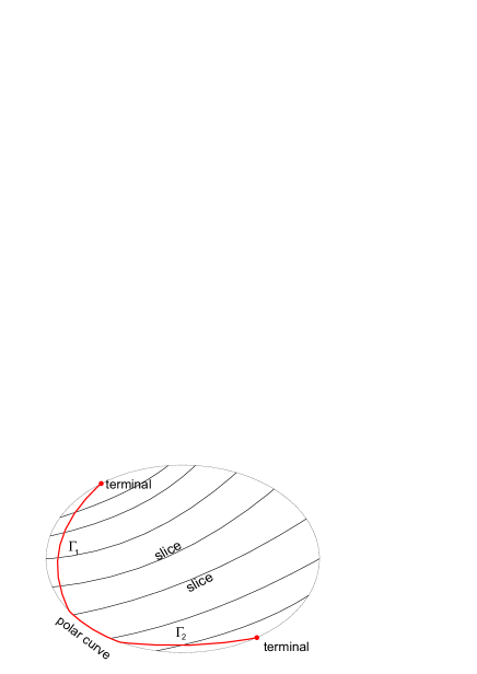
Figure 1. The space $\overline{M^{C}}(L)$, the polar curve $\Gamma$, and its components $\Gamma_{1}$ and $\Gamma_{2}$.

The polar curve is a piecewise analytic curve homeomorphic to a line segment. Its endpoints are the terminals. The polar curve may also contain some segments lying on the boundary of $\overline{M^{C}}(L)$. The intersection of the polar curve with the interior part $M^{C}(L)$ is a finite set of connected components $\Gamma_{i}$.

Since all critical points of $E$ belong to the polar curve, to prove Theorem 2 it suffices to show that $E|_{\Gamma}$ has a single critical point in $\Gamma$.

Proposition 2.

The potential $E|_{\Gamma}$ has a unique critical point in each of the connected components $\Gamma_{i}$ of the polar curve $\Gamma$.∎

With these ingredients at hand, we are ready to prove the main result.

Proof of Theorem 2

Let us start with the most symmetric case: the equilateral linkage and equal charges. We prove that $E$ has a unique critical point in $\overline{M^{C}}(L)$.

Indeed, each slice $X_{k}$ contains an axial symmetric configuration, that is, there exists a convex polygon $A_{1}A_{2}A_{3}A_{4}A_{5}$ such that:

$$|A_{3}A_{5}|=k,$$

$$\angle A_{2}A_{3}A_{4}=\angle A_{4}A_{5}A_{1},\ \ \angle A_{1}A_{2}A_{3}=\angle A_{5}A_{1}A_{2}.$$

By symmetry reasons, $A_{1}...A_{5}$ is a critical point, and therefore, (the unique) minimum point of the potential $E$ restricted to $X_{k}$. If $X_{k}$ is not a terminal point, the critical point lies in the relative interior of $X_{k}$. Therefore, for this particular case, the polar curve lies in the space $M^{C}(L)$, and by Proposition 2 we obtain the result for the equilateral pentagon and equal charges.

For an arbitrary pentagonal linkage $L$ and arbitrary (positive) charges, we use reductio ad absurdum. Assume that $\Gamma$ has more than one component, and $E$ has more than one critical points. We start continuously deforming the lengths and the charges aiming to the above symmetric linkage. Let us inspect the behavior of the critical points during the deformation. During this process all objects change continuously: the spaces $M(L)$ and $M^{C}(L)$, the slices $X_{k}$, the curve $\Gamma$ and the critical points. The number of components of $\Gamma$ can increase, but also decrease (as soon as the polar curve crosses the boundary). In the beginning of the deformation we have more than one critical points, whereas at the end the critical point is unique. The confluence of critical points cannot happen in the interior, since then two branches of $\Gamma$ have to be connected, but the limits of the critical points are distinct on that new branch unless they meet at the boundary. However two critical points on one branch is impossible by Proposition 2.

Moreover, it is proven in [10] that $E$ has no critical points on the boundary of $\overline{M^{C}}(L)$. This means that change of the number of critical points is not possible, so from the beginning we have only one critical point which is the minimum. ∎

5. Coulomb control of pentagonal linkages

For a generic pentagonal linkage, we put charges $s$ and $t$ to the vertices 5 and 3 respectively. For this case we have

$$E=\frac{q_{1}q_{4}}{d_{14}}+\frac{q_{2}q_{4}}{d_{24}}+\frac{q_{1}t}{d_{13}}+\frac{q_{2}s}{d_{25}}+\frac{st}{d_{35}}.$$

Now we wish to understand whether two charges can provide a complete control of convex pentagons. We begin with presenting a simple but conceptually important general observation valid for arbitrary polygonal linkages. This observation makes essential use of the specific form of Coulomb interaction and underlies much of the further discussion.

Proposition 3.

For any $n$-gonal linkage $L$ and any configuration $P\in M(L)$, the stabilizing charges for $P$ are solutions to a system of $n-3$ quadratic equations in $n$ unknowns with the coefficients algebraically expressible through the lengths $d_{ij}$ of the diagonals of $P$.

Proof. The proof is obtained by a standard use of the Lagrange multipliers method for constrained optimization of $E$ as a function of diagonals $d_{ij}$. In our case the number of variables $d_{ij}$ is equal to $k(n)=n(n-3)/2$. It is also easy to see that the number of independent constraints $D_{j}=0$ given by the Cayley-Menger relations for the diagonals is equal to $l(n)=(n-2)(n-3)/2$. Following prescriptions of the Lagrange method we consider a $(l(n)+1)\times k(n))$ functional matrix $J(P)$ having the gradient of target function $E_{q}$ as the first row, and gradients of constraints $D_{j}=0$ as the remaining rows. Notice that the values of charges $q_{j}$ appear only in the first row.

According to Lagrange criterion a system of charges $q$ yields a constrained critical point of $E$ on $M(L)$ if and only if the rank of $J(P)$ is not maximal. In other words, all
$(l(n)+1)\times(l(n)+1)$-minors of $J(P)$ should vanish at point $P$ which gives us a system of algebraic equations $S(n)$ for $q$ each of which is of degree not exceeding two. By linear algebra the number of independent equations in the system $S(n)$ is equal to $n-3$. The statement about coefficients can be verified directly.

∎

For a given $P\in M(L)$, let us denote by $Stab(P)$ the set of solutions to $S(n)$, i.e. the set of all charges stabilizing $P$. For obvious reasons, one may await that generically $Stab(P)$ is three-dimensional and it is easy to see that this is true for $n=4$. Indeed, in this case we have just one homogeneous quadratic equation in four unknowns $q_{i}$ of the form $Aq_{1}q_{3}+Bq_{2}q_{4}$. It follows that the solution set $Stab(P)$ is a cone over the one-sheeted two-dimensional hyperboloid. We add that similar results can be obtained for $n\geq 5$ using a general method for geometric and topological investigation of intersections of real quadrics developed in [1].

In general, the structure of $Stab(P)$ can vary from point to point, which makes it unclear how to navigate from one configuration to another one. Developing effective navigation would be easier if the sets of available charges were finite. For dimensional reasons the number of solutions to $S(n)$ may be finite if we reduce the number of unknowns (charges) to $n-3$. So it becomes natural to suggest that Coulomb control should be possible if the number of controlling charges is $n-3$, which will be assumed from now. In this setting Proposition 3 yields a modified system $S^{\prime}(n)$ and a universal upper estimate for the number of stabilizing charges which follows merely from Bezout theorem.

Lemma 1.

If $Stab(P)$ is finite then the number of stabilizing charges for $P$ does not exceed $2^{n-3}$. ∎

Examining the structure of system $S^{\prime}(5)$ we conclude that if $Stab(P)$ is finite then its cardinality in fact does not exceed two. The reason is that if the controlling charges are not neighboring then the system $S^{\prime}(5)$ consists of one linear and one quadratic equation. In this case explicit expressions for the coefficients can be found in Section (6.4).

Moreover, if we only consider convex pentagons with two controlling charges then it turns out that there exists exactly one pair of positive charges stabilizing $P$, which is the desired situation for our purposes. To prove the latter fact we need one more lemma.

Lemma 2.

[10] For $st<0$, a convex pentagon is never a critical point of $E$. ∎

Theorem 3.

For each convex configuration $P$ of a pentagonal linkage, there exists exactly one $(s,t)\in({\mathbb{R}}_{>0})^{2}$ such that $P$ is a critical point for the charges $(s,t)$.∎

We are now able to explicate the complete control for convex configurations of arbitrary pentagonal linkage, which is the main conceptual result of this paper.

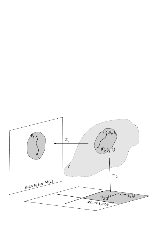
Figure 2. The critical space $C$, the state space and the control space.

We describe first our system in the general context of state space and control space. Our state space is $M(L)$, the space of pentagons with length vector $L$. The control space is the subspace of charges $(q_{1},q_{2},t,q_{4},s)$. So we work with $\mathbb{R}^{2}$ as control space. Given a potential function

$$E=E_{q}:M(L)\times\mathbb{R}^{2}\rightarrow\mathbb{R},$$

which maps $(P,q)$ to $E_{q}(P)$, one can consider the critical surface $C:=\{(P,q)|\nabla_{P}E=0\}.$ We also consider the subset of minima $C_{min}$.

The restriction to $C$ of the projection to each of the two factors of $M(L)\times\mathbb{R}^{2}$ gives us two maps: $\pi_{1}:C\rightarrow M(L)$ and $\pi_{2}:C\rightarrow\mathbb{R}^{2}$. Generically $\pi_{2}$ is a finite cover which is a local diffeomorphism away from the bifurcation set in $\mathbb{R}^{2}$. A main question is now if it is possible to connect the two configuration $P_{0}$ and $P_{1}$ by the lift (via $\pi_{1}$) of a path in the control space; if possible through the space $C_{min}$. If so, it is important to construct such a path, which we could call an explicit control to navigate from $P_{0}$ to $P_{1}$.

Theorem 2 about the uniqueness of the absolute minimum gives an affirmative answer if $P_{0}$ and $P_{1}$ are convex. Indeed $(\pi_{2})^{-1}\circ\pi_{1}$ is a bijection between $M^{C}(L)$ and ${\mathbb{R}}_{>0}^{2}$.

The corresponding algorithm to connect $P_{0}$ and $P_{1}$ can be described more precisely as follows. First, we calculate the starting and target stabilizing charges $(s_{0},t_{0})$ and $(s_{1},t_{1})$ using formulae coming from the proof of Theorem 6.4 in Section 6.4. Next, we choose a path joining $(s_{0},t_{0})$ and $(s_{1},t_{1})$ in the control space $\mathbb{R}_{>0}^{2}$. So if we continuously change the values of stabilizing charges along the chosen path the configuration will move to the target configuration through convex configurations without meeting a bifurcation point.

We summarize the above as follows.

Theorem 4.

Assume that a pentagonal linkage $L$ is charged by $(q_{1},q_{2},t,q_{4},s)$, where $q_{1},q_{2},q_{4}$ are some fixed positive charges. For any starting convex configuration $P_{0}\in M^{C}(L)$ together with any target convex configuration $P_{1}\in M^{C}(L)$, there exists an explicit control by two positive ruling charges $(s,t)$ which yields a path between $P_{0}$ and $P_{1}$ lying in $M^{C}(L)$.

Remark 1.

Since there exist infinitely many paths joining the starting and target stabilizing charges in the parameter space, several natural problems may now be formulated and explored in our setting. In particular, one can consider various problems in the spirit of optimal control. For example, since there exist various natural Riemannian metrics on the configuration space one can investigate which connecting path in parameter space gives the shortest path in the configuration space. Thinking of linkage as a device performing certain task one may wish to specify a path in the working space of a certain vertex, say, to avoid collision with an obstacle. Further examples of such problems can be easily formulated and will be discussed elsewhere.

Remark 2.

It seems worthy of noting that placing the controlling charges at adjacent vertices the situation becomes worse. Namely, we will not be able to reach all of the convex polygons (see [10]). For instance, we will never be able to have two vertices simultaneously aligned for an equilateral pentagon. By continuity reasons an entire neighborhood of such a polygon becomes unreachable.

6. Proofs

6.1. Notation and applications of Cayley-Menger determinant’s derivatives

We start with an elementary application of Theorem 1 about Cayley-Menger determinant.

Assume that we are given five points $A_{1},...,A_{5}$ in the space ${\mathbb{R}}^{3}$. Let us introduce some ad hoc notation convenient for our purposes:

$$a_{i}:=|A_{i}A_{i+1}|,$$

$$b_{i}:=|A_{i-1}A_{i+1}|,$$

$$x_{i}=b_{i}^{2},$$

where we treat the indices modulo five.

We think of $a_{i}$ as the edges and of $b_{i}$ as diagonals of the pentagon $A_{1},...,A_{5}$. Notice that we permit that the pentagon may be non-planar and non-convex.

We also need the squared diagonals $x_{i}$ which will play the role of variables.

Let $D_{i}$ be the Cayley-Menger determinant for the vertices of quadrilateral which is obtained by cutting of a triangle along $i$-th diagonal. For example, $D_{4}$ is the Cayley-Menger determinant for the quadruple $A_{1},A_{2},A_{3},A_{5}$:

$$D_{4}=\begin{vmatrix}0&1&1&1&1\\ 1&0&a_{1}^{2}&x_{2}&a_{5}^{2}\\ 1&a_{1}^{2}&0&a_{2}^{2}&x_{1}\\ 1&x_{2}&a_{2}^{2}&0&x_{4}\\ 1&a_{5}^{2}&x_{1}&x_{4}&0\\ \end{vmatrix}.$$

Applying Theorem 1 in this situation we get several useful equalities.

Lemma 3.

Assume that $A_{1},...,A_{5}$ are coplanar points. Then we have:

$$\frac{1}{2}\frac{\partial}{\partial x_{2}}D_{4}=-16S_{125}S_{235}.$$

$$\frac{1}{2}\frac{\partial}{\partial x_{4}}D_{4}=+16S_{125}S_{123}.$$

$$\frac{1}{2}\frac{\partial}{\partial x_{1}}D_{4}=-16S_{123}S_{135}.\qed$$

6.2. Proof of Proposition 1.

Throughout the paragraph we fix $b_{4}$ and parameterize the slice $X_{k}$ by $x_{2}$. In this setting the lengths of diagonals $b_{i}$, the squared lengths of diagonals $x_{i}$, and the restriction of the potential $E|_{X_{k}}$ are the functions in the variable $x_{2}$. All derivatives (denoted by ”prime”) mean derivatives with respect to $x_{2}$. For instance, we write $(b_{1})^{\prime}=\frac{db_{1}}{dx_{2}}.$

Lemma 4.

1. $$(-x_{1})^{\prime}=\frac{S_{125}}{S_{123}}\cdot\frac{S_{235}}{S_{135}}$$

2. $$(-x_{3})^{\prime}=\frac{S_{234}}{S_{135}}\cdot\frac{S_{125}}{S_{123}}$$

3. $$(x_{5})^{\prime}=\frac{S_{145}}{S_{135}}.$$

Proof follows from Lemma 3 by using the implicit differentiation formula. ∎

Lemma 5.

For a fixed slice $X_{k}$, we have $(b_{1})^{\prime}<0$, $(b_{3})^{\prime}<0$, $(b_{5})^{\prime}>0$ on the relative interior of $X_{k}$. This implies that $b_{1}\downarrow$, $b_{3}\downarrow$, $b_{5}\uparrow$.

Proof follows from Lemma 4.∎

Lemma 6.

For a fixed slice $X_{k}$, we have

1. $-(x_{1})^{\prime\prime}>0$

2. $-(x_{5})^{\prime\prime}>0$

3. $\frac{(x_{3})^{\prime}}{(x_{1})^{\prime}}\uparrow$

Proof.

(1) follows from second order relation between the diagonals of quadrilateral, see [10].

The statement (2) can be proven the same way as (1).

By Lemma 4,

$$\frac{(x_{3})^{\prime}}{(x_{1})^{\prime}}=\frac{S_{234}}{S_{235}}.$$

The statement (3) follows now from direct computation of the derivative.∎

Lemma 7.

For a fixed slice $X_{k}$, we have $E|_{X_{k}}^{\prime\prime}>0$ on the relative interior of $X_{k}$.

Proof.

The Coulomb potential for the pentagonal linkage writes as:

$$E=c_{25}b_{1}^{-1}+c_{13}b_{2}^{-1}+c_{24}b_{3}^{-1}+c_{35}b_{4}^{-1}+c_{14}b_{5}^{-1}.$$

The derivative of the potential along the slice $X_{k}$ writes as:

$$E|_{X_{k}}^{\prime}=c_{25}b_{1}^{-3}(-x_{1})^{\prime}+c_{24}b_{3}^{-3}(-x_{3})^{\prime}-c_{13}b_{2}^{-3}-c_{14}b_{5}^{-3}(x_{5})^{\prime}.$$

Using the fact that $(x_{1})^{\prime}<0$, we can rewrite this formula as:

$$E|_{X_{k}}^{\prime}=(-x_{1})^{\prime}\Big{(}c_{25}b_{1}^{-3}+c_{24}b_{3}^{-3}\frac{(-x_{3})^{\prime}}{(-x_{1})^{\prime}}\Big{)}-c_{13}b_{2}^{-3}-c_{14}b_{5}^{-3}(x_{5})^{\prime}.$$

To prove that $E^{\prime\prime}>0$ it suffices to show that:

$$(-x_{1})^{\prime}>0,$$

$$\Big{(}c_{25}b_{1}^{-3}+c_{24}b_{3}^{-3}\frac{(-x_{3})^{\prime}}{(-x_{1})^{\prime}}\Big{)}>0,$$

$$(-x_{1})^{\prime\prime}>0,$$

$$\Big{(}c_{25}b_{1}^{-3}+c_{24}b_{3}^{-3}\frac{(-x_{3})^{\prime}}{(-x_{1})^{\prime}}\Big{)}\uparrow,$$

$$(-c_{13}b_{2}^{-3})\uparrow,$$

$$(-c_{14}b_{5}^{-3}(x_{5})^{\prime})\uparrow.$$

All these statements we know from Lemma 5 and Lemma 6. ∎

Lemma 7 implies Proposition 1 straightforwardly since $E$ is strictly convex (as the function in the variable $x_{2}$) on each of the slices.

6.3. Proof of Proposition 2

As was already mentioned, $M^{C}(L)$ is a two-dimensional closed disk. We embed $M^{C}(L)$ in ${\mathbb{R}}^{5}$ by mapping each configuration to the squared lengths of its diagonals $x_{1},\dots,x_{5}$:

$$\Phi:M(L)\rightarrow\mathbb{R}^{5}.$$

This mapping sends $M^{C}(L)$ to its image bijectively so this is indeed an embedding. The mapping extends by the same rule to the entire configuration space. However on the entire configuration space it is not injective.

Now we think of $E$ as of a function defined on ${\mathbb{R}}^{5}$.

$$E=\frac{c_{25}}{b_{1}}+\frac{c_{13}}{b_{2}}+\frac{c_{24}}{b_{3}}+\frac{c_{35}}{b_{4}}+\frac{c_{14}}{b_{5}}.$$

We will deal with the signs of components of its gradient. As a matter of fact they all are negative:

$$\nabla E=-\frac{1}{2}\Big{(}\frac{c_{52}}{(b^{2}_{1})^{\frac{3}{2}}},\frac{c_{13}}{(b^{2}_{2})^{\frac{3}{2}}},\frac{c_{24}}{(b^{2}_{3})^{\frac{3}{2}}},\frac{c_{35}}{(b^{2}_{4})^{\frac{3}{2}}},\frac{c_{41}}{(b^{2}_{5})^{\frac{3}{2}}}\Big{)}\in[-;-;-;-;-].$$

Here we denoted by $[-;-;-;-;-]$ the set ${\mathbb{R}}_{-}\times{\mathbb{R}}_{-}\times{\mathbb{R}}_{-}\times{\mathbb{R}}_{-}\times{\mathbb{R}}_{-}$. In the sequel we use analogous notations regarding various combinations of signs of expressions in question.

Let $\gamma(t)=(\gamma_{1}(t),\gamma_{2}(t),\gamma_{3}(t),\gamma_{4}(t),\gamma_{5}(t))$, where $t\in[0,1]$ be a $C^{2}$-smooth curve in ${\mathbb{R}}^{5}$. Later we shall assume that $\gamma$ is the polar curve but now we consider just any smooth curve. We have

$$E(\gamma(t))=\sum{\frac{c_{ij}}{(\gamma_{k})^{\frac{1}{2}}}},$$

where the sum is over all triples such that $i+1=k(mod\,5),\ k+1=j(mod\,5)$. We denote by prime ^′ the derivative $\frac{d}{dt}$ and compute

$$E(\gamma(t))^{\prime}=-\frac{1}{2}\sum{\frac{c_{ij}(\gamma_{k})^{\prime}}{(\gamma_{k})^{\frac{3}{2}}}},$$

$$E(\gamma(t))^{\prime\prime}=\frac{3}{4}\sum{\frac{c_{ij}[(\gamma_{k})^{\prime}]^{2}}{(\gamma_{k})^{\frac{5}{2}}}}-\frac{1}{2}\sum{\frac{c_{ij}(\gamma_{k})^{\prime\prime}}{(\gamma_{k})^{\frac{3}{2}}}}.$$

From this we conclude that if the function

$$-\frac{1}{2}\sum{\frac{c_{ij}(\gamma_{k})^{\prime\prime}}{(\gamma_{k})^{\frac{3}{2}}}}=\langle\nabla E,(\gamma)^{\prime\prime}\rangle$$

is non-negative on the curve $\gamma$, then $E$ has a single critical point on the curve $\gamma$.

We remind that we denote by $D_{1}$ the Cayley-Menger determinant for the points $A_{2},A_{3},A_{4},A_{5}$, denote by $D_{2}$ the Cayley-Menger determinant for for the points $A_{1},A_{3},A_{4},A_{5}$, and so on.

The system

$$D_{1}=D_{2}=...=D_{5}=0$$

defines a surface which contains the image of $M^{C}(L)$ under the above described mapping.

Let us consider the function $D_{2}$ separately. It is a polynomial of degree $3$ in variables $x_{2},x_{4},x_{5}$. It doesn’t depend on $x_{1},x_{3}$.

Consider an open 3-arm $R$ with edgelengths $a_{3},a_{4},a_{5}$. It is a subchain of our $5$-linkage. The configuration space $M(R)$ of the arm is homeomorphic to the $2$-torus.

We map the configuration space of the arm to ${\mathbb{R}}^{3}$ by mapping each configuration to the squared lengths of its three diagonals $b_{4},b_{5}$ and $b_{2}$:

$$\Phi_{2}:M(R)\rightarrow\mathbb{R}^{3}.$$

The image of $\Phi_{2}$ belongs to the set $D_{2}=0$.

We denote by $M^{C}(R)$ those configurations of the arm that are subconfigurations of some element of $M^{C}$, that is, that are extendable to a convex pentagon.

Lemma 8.

1. $\Phi_{2}$ maps $(M^{C}(R))$ to its image bijectively.

2. $\Phi_{2}(M^{C}(R))$ is a convex surface (with boundary) in ${\mathbb{R}}^{3}$.

3. The map $\Phi_{2}$ on $M^{C}(R)$ has maximal rank except for aligned configurations.

Proof. The surface $\Phi_{2}(M(R))$ is a closed surface contained in $D_{2}=0$. The surface $\Phi_{2}(M(R))$ bounds in ${\mathbb{R}}^{3}$ some body. The image of $\Phi_{2}$ belongs to the set $D_{2}=0$. $D_{2}$ is a polynomial of degree three, therefore each generic line intersects $D_{2}=0$ at at most three points. Since a line intersects a closed surface at an even number of points, each generic line intersects $\Phi_{2}(M(R))$ at most at two points. ∎

Notice that this surface is contained in a ”box” in the positive octant.

From Theorem 1 we know the signs of all entries of all the $D_{i}$. For example,

$$\nabla D_{2}=(0;\ 16S_{345}S_{145};\ 0;\ -16S_{134}S_{145};\ -16S_{345}S_{135}).$$

We present all these signs in the following table:

$\nabla D_{1}$	$+$	0	$-$	$-$	0
$\nabla D_{2}$	0	+	0	$-$	$-$
$\nabla D_{3}$	$-$	0	+	0	$-$
$\nabla D_{4}$	$-$	$-$	0	+	0
$\nabla D_{5}$	0	$-$	$-$	0	+

Lemma 9.

The gradient $\nabla D_{2}$ is the inner normal vector of the surface $D_{2}=0$. Similar statements hold for other $D_{i}$.

Proof. It is sufficient to check if the gradient points inside or outside for one point only. We assume that we pick a pentagon without any aligned edges. We reduce the dimension as follows. First fix $x_{2}$ and after that $x_{4}$. There are only two quadrilaterals satisfying this condition: one non-convex and one convex (which has bigger $x_{5}$). The intersection with the convex body is an interval. The $x_{5}$ component of the gradient is there negative, so the gradient vector points inside. ∎

Remark 3.

The curve $\Gamma\cap M^{C}(L)$ is given by $E^{\prime}=0$ and therefore is an algebraic curve. (We remind that $E^{\prime}$ is the derivative of $E$ along the slice $X_{k}$ parameterized by $x_{2}$). Lemma 7 claims that $E^{\prime\prime}>0$ on $X_{k}$. Hence, we conclude (with the implicit function theorem) that $\Gamma\cap M^{C}(L)$ is a smooth curve which intersects $X_{k}$ transversally.

Let $\gamma(t)=\gamma(x_{4})$ parameterize the image $\Phi(\Gamma)$ of the polar curve.

We are now able to prove Proposition 2 by establishing the inequality

$$\langle\nabla E,\gamma^{\prime\prime}\rangle\geq 0\hbox{ on each of the branches $\Gamma_{j}$.}$$

Assume that a point $\gamma(t)$ does not lie on the boundary of $\Phi(M^{C})$. The curve $\gamma$ lies on $\Phi(\overline{M^{C}(L)})$ which is the part of the convex component of $D_{i}=0$ for each $i$. As we explained above, this component of $D_{i}=0$ is the boundary of some convex body, so by the Darboux formulae for the normal curvature we have:

$$\langle\gamma(t)^{\prime\prime};\nabla D_{i}\rangle\geq 0$$

Let now $\zeta$ be a tangent vector of the slice at the point $\gamma(t)$. By Lemma 5 we can assume that

$$\zeta\in[-;+;-;0;+].$$

By the definition of polar curve we have $\langle\nabla E,\zeta\rangle=0$, and obviously $\langle\nabla D_{i},\zeta\rangle=0$. To show that $\langle\nabla E;\gamma(t)^{\prime\prime}\rangle\geq 0$, it suffices to show that $\langle\nabla E;\gamma(t)^{\prime\prime}+\lambda\zeta\rangle\geq 0$ for some $\lambda$. For any $\lambda$, we have already shown that $\langle\nabla D_{i};\gamma(t)^{\prime\prime}+\lambda\zeta\rangle\geq 0$.

Since $\gamma(t)$ is parameterized by $x_{4}$, we have $\gamma(t)^{\prime\prime}\in[*;*;*;0;*]$, where $*$ denotes entries of unknown signs. Since $\langle\nabla D_{4};\gamma(t)^{\prime\prime}\rangle\geq 0$, only three cases are possible:

$$\gamma(t)^{\prime\prime}\in[-;-;*;0;*],\ \ \gamma(t)^{\prime\prime}\in[+;-;*;0;*],\ \hbox{ and }\gamma(t)^{\prime\prime}\in[-;+;*;0;*]$$

.

We treat these cases separately.

1. The first case is simple: since $\langle\nabla D_{1};\gamma(t)^{\prime\prime}\rangle\geq 0$, $\langle\nabla D_{2};\gamma(t)^{\prime\prime}\rangle\geq 0$ we have $\gamma(t)^{\prime\prime}\in(-;-;-;0;-)$, and $\langle\nabla E;\gamma(t)^{\prime\prime}\rangle\geq 0$, since $\nabla E\in(-,-,-,-,-)$. This completes the proof of Proposition 2.

2. In the second case we use $\langle\nabla D_{2};\gamma(t)^{\prime\prime}\rangle\geq 0$ and get $\gamma(t)\in(+;-;*;0;-)$. Here we have two cases: $\gamma(t)^{\prime\prime}\in(+;-;+;0;-)$ and $\gamma(t)^{\prime\prime}\in(+;-;-;0;-)$. Assume we have $\gamma(t)^{\prime\prime}\in(+;-;+;0;-)$ (the other case is treated similarly). Let us take $\gamma(t)^{\prime\prime}+\lambda\zeta$ and look how the signs change when we continuously increase $\lambda$ from $0$ to $+\infty$. We start from $(+;-;+;0;-)$ and go to $\zeta\in(-;+;-;0;+)$, which means that all the entries (except for $0$) change their signs. Let us enumerate the signs this way: $(+_{1};-_{2};+_{3};0;-_{5})$. The inequality $\langle\nabla D_{4};\gamma(t)^{\prime\prime}+\lambda\zeta\rangle\geq 0$ implies that the first sign changes before the second. The inequality $\langle\nabla D_{1};\gamma(t)^{\prime\prime}+\lambda\zeta\rangle\geq 0$ implies that the third sign changes before the first. $\langle\nabla D_{2};\gamma(t)^{\prime\prime}+\lambda\zeta\rangle\geq 0$ implies that the second sign changes before the fifth. So at some moment we necessarily have
   $\gamma(t)^{\prime\prime}+\lambda\zeta\in(-;-;-;0;-)$. Then $\langle\nabla E;\gamma(t)^{\prime\prime}+\lambda\zeta\rangle\geq 0$, which implies
   $\langle\nabla E;\gamma(t)^{\prime\prime}\rangle\geq 0$, and we are done.

3. The third case is treated similarly to the second one.

The proof of Proposition 2 is now completed.∎

6.4. Proof of Theorem 3.

The equilateral case was already proven in [10]. We follow its proof. We rewrite potential in the form

$$E=\frac{q_{1}q_{4}}{b_{5}}+\frac{q_{2}q_{4}}{b_{3}}+\frac{q_{1}t}{b_{2}}+\frac{q_{2}s}{b_{1}}+\frac{st}{b_{4}}.$$

Take now the diagonals $b_{4}$ and $b_{2}$ as local coordinates in a neighborhood of $P$.

The polygon $P$ is a critical point of $E$ means that $dE$ vanishes:

$$-\frac{\partial E}{\partial b_{4}}=\frac{q_{1}q_{4}\alpha_{1}}{b_{5}^{2}}+\frac{q_{2}q_{4}\beta_{1}}{b_{3}^{2}}+\frac{sq_{2}\gamma_{1}}{b_{1}^{2}}+\frac{st}{b_{4}^{2}}=0,$$

and

$$-\frac{\partial E}{\partial b_{2}}=\frac{q_{1}q_{4}\alpha_{2}}{b_{5}^{2}}+\frac{q_{2}q_{4}\beta_{2}}{b_{3}^{2}}+\frac{q_{1}t}{b_{2}^{2}}+\frac{q_{2}s\gamma_{2}}{b_{1}^{2}}=0,$$

where

$$\alpha_{1}=\partial b_{5}/\partial b_{4},\ \beta_{1}=\partial b_{3}/\partial b_{4},\ \ \gamma_{1}=\partial b_{1}/\partial b_{4},\hbox{ \ and}$$

$$\alpha_{2}=\partial b_{5}/\partial b_{2},\ \beta_{2}=\partial b_{3}/\partial b_{2},\ \ \gamma_{2}=\partial b_{1}/\partial b_{2}\;.$$

We get a system in two variables $s$ and $t$ which reduces to the following quadratic equation in $s$:

$$A+Bs+Cs^{2}=0$$

with

$$A=\frac{q_{1}q_{4}\alpha_{1}}{b_{5}^{2}}+\frac{q_{2}q_{4}\beta_{1}}{b_{3}^{2}},$$

$$B=\frac{q_{2}\gamma_{1}}{b_{1}^{2}}-\frac{b_{2}^{2}}{b_{4}^{2}}(\frac{q_{4}\alpha_{2}}{b_{5}^{2}}+\frac{q_{2}q_{4}\beta_{2}}{q_{1}b_{3}^{2}}),$$

$$\hbox{and \ \ \ }C=-\frac{b_{2}^{2}\gamma_{2}q_{2}}{q_{1}b_{4}^{2}b_{1}^{2}}.$$

Since $AC$ is negative by Lemma 4, the equation has exactly one real positive solution $s$. By Lemma 2, $t$ is also positive, which completes the proof.

7. Concluding remarks

By Proposition 3 for any $n$-gon we get a system $S(n)$ of quadratic equations for the stabilizing charges. The existence and structure of real solutions to this system can be analyzed using topological methods of real algebraic geometry [1]. Finding the number of positive solutions to the reduced system $S^{\prime}(n)$ is also possible using methods of [2]. So it is still unclear whether a similar Coulomb control is possible for bigger number of edges. However, our expectations are: (1) the Coulomb potential has a unique critical point (which is the global minimum) in the domain of convex configurations, (2) for a complete control, the non-ruling charges should not be put at three consecutive vertices, and (3) a convex configuration may have several collections of positive stabilizing charges.

Theorem 3 implies that we can navigate from any convex configuration to another convex configuration along any path joining their stabilizing charges in the space of charges. Since the space of charges is convex, one can use just the segment joining the stabilizing charges. It will be interesting to visualize the arising movement of linkage in the configuration space. This enables one to consider several natural versions of the optimal control problem for vertex-charged pentagonal linkages in various contexts.

References

- [1] A. Agrachev, Homology of intersections of real quadrics, Sov. Math. Dokl. 37, 1988, 493-496.
- [2] A.Agrachev, L.Lerano, Systems of quadratic inequalities, J. London Math. Soc. 105:3, 2012, 622-660.
- [3] R.Connelly, E.Demaine, Geometry and topology of polygonal linkages, Handbook of discrete and computational geometry, 2nd ed. CRC Press, Boca Raton, 2004, 197-218.
- [4] J.Cors, G.Roberts, Four-body co-circular central configurations, Nonlinearity 25, No.2, 2012, 343-348.
- [5] O. Dziobek, Uber einen Merkwurdigen Fall von Vierkoerper problem, Astron. Nachrichten, 152, 1900, 33-46.
- [6] M. Farber, Invitation to topological robotics, European Mathematical Society, 2008.
- [7] M.Hampton, Concave central configurations in the four-body problem, Doctoral Thesis, University of Washington, Seattle, 2002.
- [8] Huang Jing , Li Chuanjiang, Ma Guangfu, Liu Gang, Coulomb control of a triangular three-body satellite formation using nonlinear model predictive method, Proc. 33rd Chinese Control Conference (CCC), 2014.
- [9] G.Khimshiashvili, G.Panina, Cyclic polygons are critical points of area, Zap. Nauchn. Sem. S.-Peterburg. Otdel. Mat. Inst. Steklov. (POMI), 2008, 360, 8, 238–245.
- [10] G.Khimshiashvili, G.Panina, D.Siersma, Coulomb control of polygonal linkages, J. Dyn. Contr. Syst. 14, No.4, 2014, 491-501.
- [11] G.Khimshiashvili, G.Panina, D.Siersma, A. Zhukova, Critical configurations of planar robot arms,Centr. Europ. J. Math.11(3), 2013, 519–529.
- [12] T. Kudernac, N. Ruangsupapichat, M. Parschau, B. Mac, N. Katsonis, S. Harutyunyan, K.-H. Ernst, B. Feringa, Electrically driven directional motion of a four-wheeled molecule on a metal surface, Nature 479 (7372): 2011.
- [13] Shuquan Wang and Hanspeter Schaub, Coulomb Control of Nonequilibrium Fixed Shape Triangular Three-Vehicle Cluster, Journal of Guidance, Control, and Dynamics, Vol. 34, No. 1 (2011), 259–270.