Fast calculation of boundary crossing probabilities for Poisson processes

Abstract

The boundary crossing probability of a Poisson process with $n$ jumps is a fundamental quantity with numerous applications. We present a fast $O(n^{2}\log n)$ algorithm to calculate this probability for arbitrary upper and lower boundaries.

1 Introduction

Let $X_{1},\ldots,X_{n}$ be $n$ i.i.d. random variables drawn from $U[0,1]$ and let $\hat{F}_{n}$ be their empirical cumulative distribution function,

$$\hat{F}_{n}(t)=\frac{1}{n}\sum_{i}\mathbf{1}(X_{i}\leq t).$$

Given two arbitrary functions $g,h:[0,1]\to\mathbb{R}$, we define the corresponding two-sided non-crossing probability as

$$\Pr\left[\forall t\in[0,1]:g(t)<\hat{F}_{n}(t)<h(t)\right].$$ (1)

This probability plays a fundamental role in a wide range of applications, including the computation of $p$-values and power of sup-type continuous goodness-of-fit statistics (Kolmogorov [1], Steck [2], Noé and Vandewiele [3], Noé [4], Durbin [5], Kotel’Nikova and Khmaladze [6], Friedrich and Schellhaas [7], Khmaladze and Shinjikashvili [8]); construction of confidence bands for empirical distribution functions (Owen [9], Frey [10], Matthews [11]); change-point detection (Worsley [12]); and sequential testing (Dongchu [13]). Note that many of these applications consider a more general case, where $X_{1},\ldots,X_{n}\overset{i.i.d.}{\sim}F$ for some known continuous distribution $F$. However, this setting is easily reducible to the particular case $F=U[0,1]$ by transforming the random variables $X_{i}\mapsto F(X_{i})$ and the boundary functions as $g^{*}(t)=g(F^{-1}(t))$ and $h^{*}(t)=h(F^{-1}(t))$.

One popular approach is to estimate Eq. (1) using Monte-Carlo methods. In the simplest of these methods one repeatedly generates $X_{1},\ldots,X_{n}\sim U[0,1]$ and counts the number of times that the inequalities $g(t)<\hat{F}_{n}(t)<h(t)$ are satisfied for all $t$. This approach, however, can be extremely slow when the probability of interest is small and the sample size $n$ is large.

The focus of this paper is on the fast computation of the exact two-sided crossing probability in Eq. (1) given arbitrary boundary functions. In the one-sided case (where either $g(t)<0$ or $h(t)>1$ for all $0\leq t\leq 1$), Eq. (1) can be computed in $O(n^{2})$ operations (Noé and Vandewiele [3], Kotel’Nikova and Khmaladze [6], Moscovich et al. [14]). Even faster solutions exist for some specialized cases, such as a single linear boundary (Durbin [5]). For general boundaries, however, essentially all existing methods require $O(n^{3})$ operations (Steck [2], Durbin [15], Noé [4], Friedrich and Schellhaas [7], Khmaladze and Shinjikashvili [8]).

The main contribution of this paper is the introduction of a fast $O(n^{2}\log n)$ algorithm to compute the two-sided crossing probability for general boundary functions. This is done by investigating a closely related problem involving a Poisson process. Specifically, let $\xi_{n}(t):[0,1]\to\{0,1,2\ldots\}$ be a homogeneous Poisson process of intensity $n$ and let $g,h:[0,1]\to\mathbb{R}$ be two arbitrary boundaries. As noted in Section 3, there is a well known reduction from the probability of interest in Eq. (1) to the following two-sided non-crossing probability,

$$\Pr\left[\forall t\in[0,1]:g(t)<\xi_{n}(t)<h(t)\ |\ \xi_{n}(1)=k\right].$$ (2)

The key observation in this paper, described in Section 2, is that the recursive solution to Eq. (2) given by Khmaladze and Shinjikashvili [8] can be described as a series of at most $2n$ truncated linear convolutions involving vectors of length at most $n$. Using the Fast Fourier Transform (FFT), each convolution can thus be computed in $O(n\log n)$ operations, yielding a total running time of $O(n^{2}\log n)$.

In section 4 we present an application of the proposed method to the computation of $p$-values for a continuous goodness-of-fit statistic. Comparing the run-times of our algorithm to those of Khmaladze and Shinjikashvili [8] shows that our method yields significant speedups for large sample sizes.

Finally, since Brownian motion can be described as a limit of a Poisson process, one may apply our method to approximate the boundary crossing probability and first passage time of a Brownian motion, see for example Khmaladze and Shinjikashvili [8]. The latter quantity has multiple applications in finance and statistics (Siegmund [16], Chicheportiche and Bouchaud [17]). In this case an accurate approximation may require a fine discretization of the continuous boundaries, or equivalently a large value of $n$. Hence, fast algorithms are needed. Furthermore, our approach can be extended to higher dimensions, where it may be used to quickly approximate various quantities related to Brownian motion in $2$ or $3$ dimensions.

2 Boundary crossing probability for a Poisson process

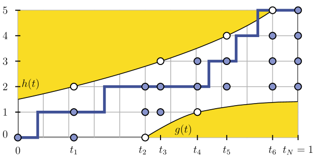
Figure 1: A two-sided boundary and a scaled empirical distribution $n\hat{F}_{n}(t)$ of $n=5$ samples. In this illustration $n\hat{F}_{n}$ happens to cross the upper boundary function $h(t)$. Empty circles mark the integer crossing points of $g(t),h(t)$ and determine discrete times $t_{1}<\ldots<t_{N}=1$ which correspond to layers of a transition graph. Note that $n\hat{F}_{n}(t)$ crosses one of the boundaries if and only if it intersects an empty circle.

In this section we describe our proposed algorithm for the fast computation of the two-sided non-crossing probability of a Poisson process, given in Eq. (2). We assume that $g(t)<h(t)$ for all $t\in[0,1]$ and that $g(0)<0<h(0)$, as otherwise the non-crossing probability is simply zero. Also, since the Poisson process is monotone, w.l.o.g. the two functions $g(t)$ and $h(t)$ may be assumed to be monotone non-decreasing. We start by describing the recursion formula of Khmaladze and Shinjikashvili [8] whose direct application yields an $O(n^{3})$ algorithm, and then show how to reduce the computational cost to $O(n^{2}\log n)$ operations.

For every integer $i\in[0,g(1)]$, let $t_{i}^{g}=\inf\{t\in[0,1]:g(t)\geq i\}$ be the first time the function $g(t)$ passes the integer $i$. Similarly for every integer $i\in[h(0),h(1)]$, let $t_{i}^{h}=\sup\{t\in[0,1]:h(t)\leq i\}$ be the last time the function $h(t)$ is bounded by $i$. Let $T(g)=\{t_{i}^{g}\}_{0\leq i\leq g(1)}$ and $T(h)=\{t_{i}^{h}\}_{h(0)\leq i\leq h(1)}$ be the set of all integer crossing times for the two functions. As illustrated in Figure 1, a non-decreasing step function $f:[0,1]\to\{0,1,2,\ldots\}$ satisfies $g(t)<f(t)<h(t)$ for all $t\in[0,1]$ if and only if it satisfies these conditions at all discrete times $t\in T(g)\cup T(h)\cup\{1\}$. Hence, to compute the probabilities in equations (1), and (2), it suffices to analyze these inequalities only at a finite set of $N=|T(g)\cup T(h)\cup\{1\}|$ times.

Definition 1.

Let $\xi_{n}(t)$ denote a one-dimensional Poisson process with intensity $n$. For any $s\in[0,1]$ and $m\in\{0,1,2,\ldots,n\}$, define $Q(s,m)$ as the probability that $\xi_{n}(s)=m$ and that $\xi_{n}$ does not cross the boundaries $g(t),h(t)$ up to time $s$. i.e.

$$Q(s,m):=\Pr\left[\forall t\in[0,s]:g(t)<\xi_{n}(t)<h(t)\text{ and }\xi_{n}(s)=m\right].$$

Of particular interest are the values $Q(1,m)$ which correspond to Poisson processes that never cross the boundaries. Clearly $Q(0,0)=1$ and $\forall m>0:Q(0,m)=0$. Let $t_{1}<\ldots<t_{N}=1$ denote the sorted set of times from $T(g)\cup T(h)\cup\{1\}$. For any $i\in\{0,\ldots,N-1\}$ and any $m\in\{0,1,2,\ldots\}$ the Chapman-Kolmogorov equations give

$$Q(t_{i+1},m)=\begin{cases}\sum_{\ell}Q(t_{i},\ell)\cdot\Pr\left[Z_{i}=m-\ell\right]&\text{ if }g(t_{i+1})<m<h(t_{i+1})\\ 0&\text{otherwise}\end{cases}$$ (3)

where $Z_{i}$ is a Poisson random variable with intensity $n(t_{i+1}-t_{i})$ and the sum is taken over all $g(t_{i})<\ell\leq m$. This formula was proposed by Khmaladze and Shinjikashvili [8] in order to compute $Q(1,n)$. All quantities up to the final time $t_{N}=1$ can be computed recursively as follows: first calculate explicitly the probabilities $Q(t_{1},0),\ldots,Q(t_{1},n)$ at time $t_{1}$. Next, calculate all probabilities at time $t_{i+1}$ using the quantities from time $t_{i}$, and so on. Since each $Q(t_{i},m)$ is a sum of up to $m+1\leq n+1$ terms and since $N\leq 2n+1$. the total run-time is at most $O(n^{3}),$ but may be smaller if the boundary functions $g(t),h(t)$ are close to each other.

Next, we describe a faster procedure. Let $Q_{t_{i}}=(Q(t_{i},0),Q(t_{i},1),\ldots,Q(t_{i},n))$ and let $\pi_{\lambda}=(\Pr\left[Z=0\right],\Pr\left[Z=1\right],\ldots,\Pr\left[Z=n\right]),$ where $Z\sim\text{Poisson}(\lambda)$. The key observation is that the vector $Q_{t_{i+1}}$ in Eq. (3) is nothing but a truncated linear convolution of the vectors $Q_{t_{i}}$ and $\pi_{n(t_{i+1}-t_{i})}$. Hence we may apply the circular convolution theorem to compute it in the following fashion:

1. Append $n$ zeros to the end of the two vectors $Q_{t_{i}}$ and $\pi_{n(t_{i+1}-t_{i})}$, denoting the resulting vectors $Q^{2n}$ and $\pi^{2n}$ respectively.

2. Compute the Fourier transform of the zero-extended vectors $\mathcal{F}\{Q^{2n}\}$ and $\mathcal{F}\{\pi^{2n}\}$.

3. Use the convolution theorem to obtain the Fourier transform of the convolution,

   $$C^{2n}=\mathcal{F}\{Q^{2n}\star\pi^{2n}\}=\mathcal{F}\{Q^{2n}\}\cdot\mathcal{F}\{\pi^{2n}\},$$

   where $\star$ denotes cyclic convolution and $\cdot$ denotes pointwise multiplication.

4. Compute the inverse Fourier transform of $C^{2n}$ to yield the vector $Q_{t_{i+1}}$

   $$Q_{t_{i+1}}(m)=\begin{cases}\mathcal{F}^{-1}\{C^{2n}\}(m)&\text{if }g(t_{i+1})<m<h(t_{i+1})\\ 0&\text{otherwise}.\end{cases}$$

Using the FFT algorithm, each Fourier Transform takes $O(n\log n)$ time. Repeating these four steps for all times $t\in T(g)\cup T(h)\cup\{1\}$ yields a worst-case total run-time of $O(n^{2}\log n)$. However, it may be much lower if the functions $g(t)$ and $h(t)$ are close to each other. For more details on the FFT and the computation of discrete convolutions, we refer the reader to Press et al. [18, Chapters 12, 13].

3 Boundary crossing probability for the empirical CDF

We now return to the problem of calculating the probability in Eq. (1), that an empirical CDF will cross prescribed upper and lower boundaries. To simplify notation, we look at the scaled function $n\hat{F}_{n}(t)$ instead of $\hat{F}_{n}(t)$, and similarly to the previous section, consider the probabilities

$$R(s,m)=\Pr\left[\forall t\in[0,s]:g(t)<n\hat{F}_{n}(t)<h(t)\text{ and }n\hat{F}_{n}(t)=m\right].$$

Let $0=t_{0}<t_{1}<\ldots<t_{N}=1$ be as before, and let

$$Z_{\ell,i}\sim\text{Binomial}\left(n-\ell,\tfrac{t_{i+1}-t_{i}}{1-t_{i}}\right).$$

The Chapman-Kolmogorov equations give the recursive relations of Friedrich and Schellhaas [7]

$$R(t_{i+1},m)=\begin{cases}\sum_{\ell}R(t_{i},\ell)\cdot\Pr\left[Z_{\ell,i}=m-\ell\right]&\text{if }g(t_{i+1})<m<h(t_{i+1})\\ 0&\text{otherwise.}\end{cases}$$ (4)

In contrast to Eq. (3), the expression for $R_{t_{i+1}}$, the vector of probabilities at time $t_{i+1}$, is not in the form of a straightforward convolution, and hence cannot be directly computed using the FFT. While not the focus of our work, we note that by some algebraic manipulations, it is possible to compute Eq. (4) using a convolution and an additional $O(n)$ operations. Instead, we present a simpler construction that builds upon the results of the previous section. To this end we recall a well-known reduction from the empirical CDF to the Poisson process (Shorack and Wellner [19, Chapter 8, Proposition 2.2]):

Lemma 1.

The distribution of the process $n\hat{F}_{n}(t)$ is identical to that of a Poisson process $\xi_{n}(t)$ with intensity $n$, conditioned on $\xi_{n}(1)=n$.

According to this lemma, the non-crossing probability of an empirical CDF can be efficiently computed by a reduction to the Poisson case, since

$$\Pr\left[\forall t:g(t)<n\hat{F}_{n}(t)<h(t)\right]=\Pr\left[\forall t:g(t)<\xi_{n}(t)<h(t)|\xi_{n}(1)=n\right]$$ (5)

$$=\frac{\Pr\left[\forall t:g(t)<\xi_{n}(t)<h(t)\text{ and }\xi_{n}(1)=n\right]}{\Pr\left[\text{Poisson}(n)=n\right]}=\frac{Q(n,n)}{n^{n}e^{-n}/n!}$$

and $Q(n,n)$ can be computed efficiently, as described in Section 2.

4 Computing p-values for goodness-of-fit statistics

The results of the previous sections can be used to compute the $p$-value of several two-sided continuous goodness-of-fit statistics such as Kolmogorov-Smirnov, and their power against specific alternatives. Our algorithm may also be applied to one-sided statistics such as the Higher-Criticism statistic of Donoho and Jin [20].

To this end, recall the setup in the classical continuous goodness-of-fit testing problem. Let $x_{1},x_{2},\ldots,x_{n}$ be $n$ real-valued samples. We wish to assess the validity of a null hypothesis that $x_{1},\ldots,x_{n}$ are sampled i.i.d from a known (and fully specified) continuous distribution function $F$ against an unknown and arbitrary alternative $G$,

$$\mathcal{H}_{0}:x_{i}\overset{i.i.d.}{\sim}F\quad vs.\quad\mathcal{H}_{1}:x_{i}\overset{i.i.d.}{\sim}G\ \text{ with }\ G\neq F.$$

Let $u_{i}=F(x_{i})$ be the probability integral transform of the $i$-th sample, and $u_{(1)}\leq u_{(2)}\leq\ldots\leq u_{(n)}$ be the sorted sequence of transformed samples. Under the null hypothesis, each $u_{i}$ is uniformly distributed in $[0,1]$ and therefore $u_{(i)}$ is the $i$-th order statistic of a uniform distribution.

A common approach to goodness-of-fit testing is to measure the distance of the different order statistics from their expectation under the null. A classical example is the Kolmogorov-Smirnov statistic $K_{n}:=\max\{K_{n}^{-},K_{n}^{+}\}$, where $K_{n}^{-}$ and $K_{n}^{+}$ are the one-sided KS statistics, defined as

$$K_{n}^{-}=\sqrt{n}\max_{i=1,\ldots,n}\left(u_{(i)}-\frac{i-1}{n}\right),\quad K_{n}^{+}=\sqrt{n}\max_{i=1,\ldots,n}\left(\frac{i}{n}-u_{(i)}\right).$$

More generally, given a sequence of monotone-increasing functions $r_{1},\ldots,r_{n}:\mathbb{R}\to\mathbb{R}$ and a sequence of decreasing functions $s_{1},\ldots,s_{n}:\mathbb{R}\to\mathbb{R}$, one may define one-sided goodness-of-fit statistics by

$$R:=\max_{i=1,\ldots,n}r_{i}(u_{(i)})\quad\text{and}\quad S:=\max_{i=1,\ldots,n}s_{i}(u_{(i)})$$ (6)

and a two-sided statistic by

$$T:=\max\{R,S\}.$$ (7)

Statistics of this form include the supremum Anderson-Darling statistic and other weighted Kolmogorov-Smirnov statistics [1, 21], the $R_{n}$ statistic of Berk and Jones [22] and Phi-divergence supremum statistics [23]. Similarly, the one-sided Higher Criticism statistic of Donoho and Jin [20] and its variants follow the form of the one-sided statistic $S$ in Eq. (6).

It is easy to verify that $T<t$ if and only if $s_{i}^{-1}(t)<u_{(i)}<r_{i}^{-1}(t)$ holds for all $i$. Therefore, the $p$-value of $T=t$ is equal to

$$\Pr\left[T>t|\mathcal{H}_{0}\right]=1-\Pr\left[\forall 1\leq i\leq n:s_{i}^{-1}(t)<U_{(i)}<r_{i}^{-1}(t)\right],$$ (8)

where $U_{(1)},\ldots,U_{(n)}$ are the order statistics of $n$ draws from $U[0,1]$. Define two functions $g_{t}(x)$ and $h_{t}(x)$ as follows,

$$g_{t}(x)=\sum_{i=1}^{n}\mathbf{1}(r_{i}^{-1}(t)\leq x),\quad h_{t}(x)=\sum_{i=1}^{n}\mathbf{1}(s_{i}^{-1}(t)\leq x),$$

then the probability of Eq. (8) is equal to that of Eq. (5) which we can compute in time $O(n^{2}\log n)$.

4.1 Simulation Results

We evaluate the empirical run-time of our procedure for computing $p$-values of the two-sided $M_{n}$ and one-sided $M_{n}^{+}$ goodness-of-fit statistics of Berk and Jones [22]. These statistics have the form of equations (6) and (7) but with a minimum instead of a maximum (see [14, Section 3]).

To this end we wrote an efficient implementation of the proposed procedure using the FFTW3 library by Frigo and Johnson [24] and compared it to a direct implementation of the Khmaladze and Shinjikashvili [8] recursion relations (denoted ”KS 2001”). In addition, we implemented the $O(n^{2})$ one-sided algorithm of Moscovich et al. [14] (denoted ”MNS 2016”). We find that both two-sided procedures are numerically stable using standard double-precision (64-bit) floating point numbers, even for sample sizes as large as $n=250,000$. In contrast, the one-sided procedure [14] requires a careful numerical implementation using extended-precision (80-bit) floating point numbers and breaks down completely for sample sizes $n>50,000$. Figure 2 presents a runtime comparison of the three algorithms for computing one-sided and two-sided crossing probabilities.

Somewhat counter-intuitively, the one-sided case is much more expensive than the two-sided case. This is made clear by examining Eq. (3) and noting that in the one-sided case the variable $m$ has a large valid range averaging around $n/2$, whereas in the two-sided case this range is typically much smaller. In all cases, our procedure is the fastest of all 3 methods. Surprisingly, this is true even in the one-sided case where the $O(n^{2})$ procedure of Moscovich et al. [14] is asymptotically superior.

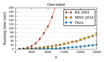
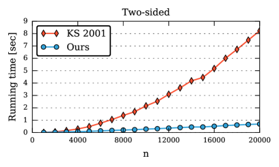
Figure 2: Runtime comparison of our algorithm compared to that of Khmaladze and Shinjikashvili [8] (KS 2001) and to the one-sided method described in Moscovich et al. [14] (MNS 2016). The boundaries were chosen such that the $p$-value of $M_{n}$, equal to its two-sided boundary crossing probability, is 5%. Note that the one-sided case is much slower to compute.

Finally, we note that for large sample sizes, one may be inclined to forgo exact computation of $p$-values and instead use the asymptotic null distribution of the particular test statistic in use (assuming it is known). However, this does not always provide an adequate approximation, particularly as in several cases the finite sample distribution converges very slowly to its limiting form. Depending on the application, even the currently best known approximations may not be sufficiently accurate. For more on this topic, see Li and Siegmund [25].

5 References

References

- Kolmogorov [1933] A. N. Kolmogorov, Sulla determinazione empirica di una legge di distribuzione, Giornale dell’instituto italiano degli attuari 4 (1933) 83–91.
- Steck [1971] G. P. Steck, Rectangle probabilities for uniform order statistics and the probability that the empirical distribution function lies between two distribution functions, The annals of mathematical statistics 42 (1) (1971) 1–11, http://doi.org/10.1214/aoms/1177693490.
- Noé and Vandewiele [1968] M. Noé, G. Vandewiele, The calculation of distributions of Kolmogorov-Smirnov type statistics including a table of significance points for a particular case, The annals of mathematical statistics 39 (1) (1968) 233–241, http://doi.org/10.1214/aoms/1177698523.
- Noé [1972] M. Noé, The calculation of distributions of two-sided Kolmogorov-Smirnov type statistics, The annals of mathematical statistics 43 (1) (1972) 58–64, http://doi.org/10.1214/aoms/1177692700.
- Durbin [1973] J. Durbin, Distribution theory for tests based on sample distribution function, SIAM, http://doi.org/10.1137/1.9781611970586, 1973.
- Kotel’Nikova and Khmaladze [1983] V. F. Kotel’Nikova, E. V. Khmaladze, On computing the probability of an empirical process not crossing a curvilinear boundary, Theory of probability & its applications 27 (1983) 640–648, http://doi.org/10.1137/1127075.
- Friedrich and Schellhaas [1998] T. Friedrich, H. Schellhaas, Computation of the percentage points and the power for the two-sided Kolmogorov-Smirnov one sample test, Statistical papers 39 (1998) 361–375, http://doi.org/10.1007/BF02927099.
- Khmaladze and Shinjikashvili [2001] E. Khmaladze, E. Shinjikashvili, Calculation of noncrossing probabilities for poisson processes and its corollaries, Advances in applied probability 33 (2001) 702–716, http://doi.org/10.1239/aap/1005091361.
- Owen [1995] A. B. Owen, Nonparametric likelihood confidence bands for a distribution function, Journal of the american statistical association. 90 (430) (1995) 516–521, http://doi.org/10.2307/2291062.
- Frey [2008] J. Frey, Optimal distribution-free confidence bands for a distribution function, Journal of statistical planning and inference 138 (2008) 3086–3098, http://doi.org/10.1016/j.jspi.2007.12.001.
- Matthews [2013] D. Matthews, Exact nonparametric confidence bands for the survivor function., The international journal of biostatistics 9 (2) (2013) 185–204, http://doi.org/10.1515/ijb-2012-0046.
- Worsley [1986] K. J. Worsley, Confidence regions and tests for a change point in a sequence of exponential family random variables, Biometrika 73 (1) (1986) 91–104, http://doi.org/10.1093/biomet/73.1.91.
- Dongchu [1998] S. Dongchu, Exact computation for some sequential tests, Sequential analysis 17 (2) (1998) 127–150, http://doi.org/10.1080/07474949808836403.
- Moscovich et al. [2016] A. Moscovich, B. Nadler, C. Spiegelman, On the exact Berk-Jones statistics and their p-value calculation, Tech. Rep., http://arxiv.org/abs/1311.3190v5, 2016.
- Durbin [1971] J. Durbin, Boundary-crossing probabilities for the Brownian motion and Poisson processes and techniques for computing the power of the Kolmogorov-Smirnov test, Journal of Applied Probability 8 (3) (1971) 431–453, http://doi.org/10.2307/3212169.
- Siegmund [1986] D. Siegmund, Boundary crossing probabilities and statistical applications, The annals of statistics 14 (2) (1986) 361–404, http://doi.org/10.1214/aos/1176349928.
- Chicheportiche and Bouchaud [2014] R. Chicheportiche, J.-P. Bouchaud, Some applications of first-passage ideas to finance, in: First-passage phenomena and their applications, http://doi.org/10.1142/9789814590297_0018, 2014.
- Press et al. [1992] W. H. Press, B. P. Flannery, S. A. Teukolsky, V. W. T., Numerical recipes in C: the art of scientific computing, Cambridge University Press, 2nd edn., http://apps.nrbook.com/c/index.html, 1992.
- Shorack and Wellner [2009] G. R. Shorack, J. A. Wellner, Empirical processes with applications to statistics, SIAM, http://doi.org/10.1137/1.9780898719017, 2009.
- Donoho and Jin [2004] D. Donoho, J. Jin, Higher criticism for detecting sparse heterogeneous mixtures, Annals of statistics 32 (3) (2004) 962–994, http://doi.org/10.1214/009053604000000265.
- Anderson and Darling [1952] T. Anderson, D. Darling, Asymptotic theory of certain ”goodness of fit” criteria based on stochastic processes, The annals of mathematical statistics 23 (2) (1952) 193–212, http://projecteuclid.org/euclid.aoms/1177729437.
- Berk and Jones [1979] R. H. Berk, D. H. Jones, Goodness-of-fit test statistics that dominate the Kolmogorov statistics, Probability theory and related fields 47 (1979) 47–59, http://doi.org/10.1007/BF00533250.
- Jager and Wellner [2007] L. Jager, J. A. Wellner, Goodness-of-fit tests via phi-divergences, Annals of statistics 35 (5) (2007) 2018–2053, http://doi.org/10.1214/0009053607000000244.
- Frigo and Johnson [2005] M. Frigo, S. G. Johnson, The design and implementation of FFTW3, Proceedings of the IEEE 93 (2) (2005) 216–231, http://doi.org/10.1109/JPROC.2004.840301.
- Li and Siegmund [2015] J. Li, D. Siegmund, Higher criticism: p-values and criticism, The Annals of Statistics 43 (3) (2015) 1323–1350, http://doi.org/10.1214/15-aos1312.